On the construction of nested space-filling designs

Abstract

Nested space-filling designs are nested designs with attractive low-dimensional stratification. Such designs are gaining popularity in statistics, applied mathematics and engineering. Their applications include multi-fidelity computer models, stochastic optimization problems, multi-level fitting of nonparametric functions, and linking parameters. We propose methods for constructing several new classes of nested space-filling designs. These methods are based on a new group projection and other algebraic techniques. The constructed designs can accommodate a nested structure with an arbitrary number of layers and are more flexible in run size than the existing families of nested space-filling designs. As a byproduct, the proposed methods can also be used to obtain sliced space-filling designs that are appealing for conducting computer experiments with both qualitative and quantitative factors.

, and

t2Supported by NNSF of China Grant 11101074 and Program for Changjiang Scholars and Innovative Research Team in University. t3Supported by NNSF of China Grant 11271205, Specialized Research Fund for the Doctoral Program of Higher Education of China Grant 20130031110002, and “131” Talents Program of Tianjin. t4Supported by NSF Grants DMS-10-55214 and CMMI 0969616.

1 Introduction

Computer experiments are widely used in science and engineering [Fang, Li and Sudjianto (2006), Santner, Williams and Notz (2003)]. A large computer program can often be run with multiple fidelities. Qian (2009), Qian, Tang and Wu (2009) and Qian, Ai and Wu (2009) introduced the concept of nested space-filing design (NSFD) for running computer codes with two levels of accuracy. A pair of NSFD $L_{1}\subset L_{2}$ are two nested designs with the small design used for the more accurate but more expensive code and the large design used for the less accurate but cheaper code. These designs have following properties:

Economy: the number of points in $L_{1}$ is smaller than the number of points in $L_{2}$;

Nested relationship: $L_{1}$ is nested within $L_{2}$, that is, $L_{1}\subset L_{2}$;

Space-filling: the points in both $L_{1}$ and $L_{2}$ achieve uniformity in low dimensions.

The nested relationship makes it easier to adjust or calibrate the differences between the two sources.

Multi-fidelity simulation modeling has received considerable attention over the past few years, especially in the computational fluid dynamics and finite element analysis communities where simulation costs are very high. For example, a finite element analysis code can be run with varying numbers of mesh sizes, resulting in multiple versions with three or more levels of accuracy. Multi-fidelity simulation modeling is a common practice in engineering. Examples include Dewettinck et al. (1999) for simulating a GlattGPC-1 fluidized-bed unit, Choi et al. (2008) for an aircraft design application and Molina-Cristóbal et al. (2010) for a submarine propulsion system application, among others. Specifically in Dewettinck et al. (1999), they reported a physical experiment and several associated computer models for predicting the steady-state thermodynamic operation point of a GlattGPC-1 fluidized-bed unit. One physical model $(T_{2,{\mathrm{exp}}})$ and three computer models $(T_{2,3},T_{2,2},T_{2,1})$ are considered. Model $T_{2,3}$, which includes adjustments for heat losses and inlet airflow, is the most accurate (i.e., producing the closest response to $T_{2,{\mathrm{exp}}}$). Model $T_{2,2}$ includes only the adjustment for heat losses, thus is the medium accurate. While model $T_{2,1}$ does not adjust for heat losses or inlet airflow and is thus the least accurate. For such experiments, it is desirable to run a multi-layer experiment using NSFDs with three or more layers, which makes it easier to model the systematic differences among the models and implies more observations are taken for less accurate experiments [cf., Haaland and Qian (2010)].

However, NSFDs with more than two layers cannot be constructed by using the methods in Qian, Tang and Wu (2009) and Qian, Ai and Wu (2009). The technical reason is the modulus projection used in Qian, Tang and Wu (2009) cannot be extended to covering more than two layers. To overcome this limitation, we present a new group-to-group projection, called the subgroup projection, in this paper and then construct several new classes of NSFDs that can accommodate nesting with an arbitrary number of layers and are more flexible in run size than existing designs of this type. The subgroup projection is based on a new decomposition of Galois fields. As far as we are aware, it is also new in algebra and may have other algebraic applications beyond design of experiments. Some families of NSFDs with more than two layers can be constructed from $(t,s)$-sequences with an infinite number of elements [Haaland and Qian (2010)]. In contrast, the proposed construction here is simpler and only involves a finite number of points. The constructed designs here can be used for multi-level fitting of nonparametric functions [Floater and Iske (1996), Fasshauer (2007), Haaland and Qian (2011)] and linking parameters in engineering [Husslage et al. (2003)], all of which involve nested designs with more than two layers.

The proposed constructions also give new families of sliced space-filling designs (SSFDs) which can be used to conduct computer experiments with both qualitative and quantitative factors [Qian, Wu and Wu (2008), Han et al. (2009), Zhou, Qian and Zhou (2011)]. Such computer experiments are often encountered in practice, though most literature on computer experiments assumes that all the input variables are quantitative. For example, Schmidt, Cruz and Iyengar (2005) described a data center computer experiment which involves qualitative factors (such as diffuser location and hot-air return-vent location) and quantitative factors (such as rack power and diffuser flow rate). For conducting such an experiment, Qian and Wu (2009) proposed to use an SSFD, say $S=(S^{\prime}_{1},\ldots,S^{\prime}_{v})^{\prime}$, with each slice $S_{i}$ being associated with a level combination of the qualitative factors. Here, when collapsed over the qualitative levels, the points of the quantitative factors achieve attractive stratification and at any qualitative level, the values of the quantitative factors are spread uniformly in a low-dimensional space. An SSFD can also be used to run a computer model in batches and conduct multiple computer models [Qian (2012), Williams, Morris and Santner (2009)]. Note that the subfield projection used in Qian and Wu (2009) for constructing SSFDs is a special case of the subgroup projection proposed in this paper, thus more SSFDs can be constructed here. Moreover, the SSFDs presented in this paper can be used to conduct computer experiments with asymmetric qualitative factors.

This paper is organized as follows. Section 2 presents some useful definitions and notation. Section 3 introduces a decomposition method of Galois fields and a new algebraic projection, which play a critical role in the proposed construction methods. Sections 4–6 provide new methods for constructing nested orthogonal arrays, sliced orthogonal arrays and nested difference matrices, along with illustrative examples. Procedures for generating NSFDs from nested orthogonal arrays and SSFDs from sliced orthogonal arrays are presented in Section 7. Comparisons with existing work and concluding remarks are given in Section 8.

2 Definitions and notation

Latin hypercube and orthogonal array-based Latin hypercube. A Latin hypercube $L=(l_{ij})$ with $n$ runs and $m$ factors is an $n\times m$ matrix in which each column is a permutation of $0,\ldots,n-1$ [McKay, Beckman and Conover (1979)]. Let $A$ be an orthogonal array $\mathit{OA}(n,m,s,t)$ with levels $0,\ldots,s-1$ [Hedayat, Sloane and Stufken (1999)]. If we replace the $q=n/s$ zeros in each column of $A$ by a permutation of $0,\ldots,q-1$, replace the $q$ ones by a permutation of $q,\ldots,2q-1$, and so on, we obtain an orthogonal array (OA)-based Latin hypercube that achieves stratification up to $t$ dimensions [Tang (1993)].

Sliced orthogonal array. Let $A$ be an $\mathit{OA}(n_{2},m,s_{2},t)$. Suppose that the rows of $A$ can be partitioned into $v$ subarrays of $n_{1}$ rows, denoted by $A_{1},\ldots,A_{v}$. Further suppose that there is a projection $\rho$ that collapses the $s_{2}$ levels of $A$ into $s_{1}$ levels with $s_{2}>s_{1}$ and $A_{i}$ becomes an $\mathit{OA}(n_{1},m,s_{1},t)$ after level-collapsing according to $\rho$. Then $A$, or more precisely $(A_{1},\ldots,A_{v};\rho)$, is a sliced orthogonal array (SOA) [Qian and Wu (2009)].

Nested orthogonal array and nested difference matrix. Qian, Tang and Wu (2009) and Qian, Ai and Wu (2009) introduced the definition of nested orthogonal array with two layers, we now extend the definition to a more general case. Suppose $A_{I}$ is an $\mathit{OA}(n_{I},m,s_{I},t)$ and $\rho_{j}$ for $j=1,\ldots,I$ are a series of projections satisfying that $\rho_{i}(\alpha)=\rho_{i}(\beta)$ implies $\rho_{j}(\alpha)=\rho_{j}(\beta)$ for $j\leq i$. Then $(A_{1},\ldots,A_{I};\rho_{1}$, $\ldots,\rho_{I})$ is called a nested orthogonal array (NOA) with $I$ layers, denoted by $\mathit{NOA}(A_{1}$, $\ldots,A_{I};\rho_{1},\ldots,\rho_{I})$, if: [(ii)]

$A_{i-1}$ is nested within $A_{i}$ for $2\leq i\leq I$, that is, $A_{1}\subset A_{2}\subset\cdots\subset A_{I}$;

$\rho_{j}(A_{i})$ is an $\mathit{OA}(n_{i},m,s_{j},t)\mbox{ for }j\leq i$, where $n_{1}<n_{2}<\cdots<n_{I}$ and $s_{1}<s_{2}<\cdots<s_{I}$. Given a difference matrix $D(r_{I},c,s_{I})$ [Bose and Bush (1952)], the concept of nested difference matrix (NDM) with $I$ layers, denoted by $\mathit{NDM}(D_{1},\ldots,D_{I};\rho_{1},\ldots,\rho_{I})$, is defined in a similar fashion.

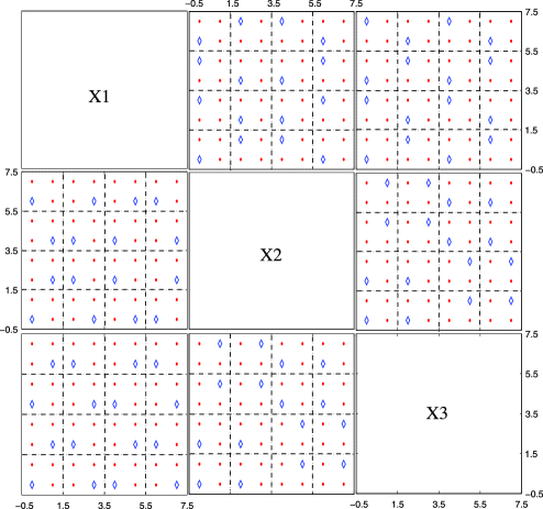
Figure 1: Bivariate projections of $A_{1}$ and $A_{2}$ with $A_{1}\subset A_{2}$, where the points labeled with both “$\diamond$” and “$\cdot$” correspond to $A_{2}$, and those labeled with “$\diamond$” correspond to $A_{1}$.

Note that the concept of NOA here is different from the one introduced in Mukerjee, Qian and Wu (2008), since the $A_{i}$ for $i=1,\ldots,I-1$ here are not necessarily OAs before the level-collapsing but can still achieve stratification on any two dimensions. This makes the construction more flexible. For example, Figure 1 presents the bivariate projections of an $\mathit{OA}(64,5,8,2)$ with levels $0,\ldots,7$, denoted by $A_{2}$, and a 16-run subset of $A_{2}$, denoted by $A_{1}$, where the points labeled with both “$\diamond$” and “$\cdot$” correspond to $A_{2}$, and those labeled with “$\diamond$” correspond to $A_{1}$ (for saving space, only the bivariate projections of the first three dimensions are presented here). Obviously, $A_{1}$ is not an OA, but it becomes an $\mathit{OA}(16,5,4,2)$ with levels $0,2,4,6$ after the level-collapsing according to the projection $\{0,1\}\rightarrow 0,\{2,3\}\rightarrow 2,\{4,5\}\rightarrow 4,\{6,7\}\rightarrow 6$, and the points of $A_{1}$ achieve stratification on the $4\times 4$ grids in any two dimensions. According to Theorem 1 of Mukerjee, Qian and Wu (2008), if an $\mathit{OA}(N,5,8,2)$ contains an $\mathit{OA}(16,5,4,2)$, then $N$ must satisfy $N\geq 96$, but here the larger OA only has $N=64$ runs if the projection is used to get the smaller OA with 16 runs. Thus, in the present paper, suitable projections are critical for the definition and construction of NOAs, and the use of projections makes the construction more flexible.

Consider two matrices $A=(a_{ij})=(a_{1},\ldots,a_{s})$ of order $r\times s$ and $B=(b_{ij})=(b_{1},\ldots,b_{v})$ of order $u\times v$, respectively. Their Kronecker sum is an $ru\times sv$ matrix

$$A\oplus B=(a_{ij}J+B)\qquad\mbox{where }J\mbox{ is the }u\times v\mbox{ matrix of ones.}$$ (1)

For $s=v$, here we introduce an operation called column-wise Kronecker sum of $A$ and $B$, given as

$$A\oplus_{c}B=(a_{1}\oplus b_{1},\ldots,a_{s}\oplus b_{s}),$$ (2)

where $\oplus$ is defined in (1). These two operations will be used to construct NOAs, SOAs and NDMs in the following sections.

Generator matrix and Rao–Hamming construction. Let $s=p^{u}$, $\mathit{GF}(p)\subseteq F_{1}\subseteq\mathit{GF}(s)$ with $|F_{1}|=m$, where $p$ is a prime number and $|F_{1}|$ denotes the cardinality of set $F_{1}$, and let $z_{j}$ be a column vector of length $k$ with the $j$th component being one and all the others being zero, $j=1,\ldots,k$. We then obtain a $k\times(m^{k}-1)/(m-1)$ matrix $Z_{1}$ by collecting all the nonzero column vectors given by

$$z=c_{1}z_{1}+\cdots+c_{k}z_{k}\qquad\mbox{where }c_{j}\in F_{1}$$ (3)

and the first nonzero entry in $(c_{1},\ldots,c_{k})$ is one. We call $Z_{1}$ a generator matrix over $F_{1}$ with $k$ independent columns. Let $Z$ be the generator matrix over $\mathit{GF}(s)$ with $k$ independent columns and take all linear combinations of the row vectors of $Z$ with coefficients from $\mathit{GF}(s)$, we then obtain an $\mathit{OA}(s^{k},(s^{k}-1)/(s-1),s,2)$. This construction is called the Rao–Hamming construction [Hedayat, Sloane and Stufken (1999), Chapter 3].

Lemma 1 follows from the Rao–Hamming construction.

Lemma 1

Let $s$ be a prime power and let $A$ be an $s^{k}\times k$ matrix whose rows consist of all the vectors $(x_{1},\ldots,x_{k})$, $x_{i}\in\mathit{GF}(s),i=1,\ldots,k$, then $AZ$ is an $\mathit{OA}(s^{k},(s^{k}-1)/(s-1),s,2)$, where $Z$ is a generator matrix over $\mathit{GF}(s)$ with $k$ independent columns.

3 A new subgroup projection

We now introduce a new projection which will play a key role in the proposed construction methods in the subsequent sections. Moreover, this new projection may have other applications in Algebra. We first present a lemma about the decomposition of Galois fields.

3.1 Decomposition of Galois fields

For a finite set $A$ of size $|A|$, put its elements in an column vector $V_{A}$ with zero being placed as the first entry if included. The following lemma paves the way for a new decomposition of Galois fields.

Lemma 2

Suppose that $G$ is a finite Abelian group with $|G|=n$. Then there exists a decomposition of $n=p^{t_{1}}_{1}\times\cdots\times p^{t_{l}}_{l}$ and cyclic groups $G_{i}$ with $|G_{i}|=p^{t_{i}}_{i}$ satisfying $V_{G}=V_{G_{1}}\oplus\cdots\oplus V_{G_{l}}$, where $p_{i}$ is a prime, $G_{i}\subset G$ and $G_{i}\cap G_{j}=\{0\}$ for $i\neq j,i,j=1,\ldots,l$.

This lemma is a direct result of the fundamental theorem of finite Abelian group which states that any finite Abelian group can be decomposed as a direct sum of cyclic subgroups of prime power order [cf. Herstein (1996), Theorem 2.10.3]. Based on Lemma 2, we have the following result.

Lemma 3

Suppose $F_{3}$ is a Galois field $\mathit{GF}(p^{u_{3}})$ and $F_{1},F_{2}$ are subgroups of $F_{3}$ under operation “$+$”. If $F_{1}$ is a subgroup of $F_{2}$ under operation “$+$”, then there exists a subgroup $T$ of $F_{2}$ under operation “$+$” satisfying $V_{F_{2}}=V_{F_{1}}\oplus V_{T}$.

Suppose $|F_{2}|=p^{u_{2}}$. By Lemma 2, there exists a decomposition of $p^{u_{2}}=p^{t_{1}}\times\cdots\times p^{t_{l}}$ and cyclic groups $G_{i}$ satisfying $V_{F_{2}}=V_{G_{1}}\oplus\cdots\oplus V_{G_{l}}$, where $|G_{i}|=p^{t_{i}}$, $G_{i}\subset F_{2}$ and $G_{i}\cap G_{j}=\{0\}$ for $i,j=1,\ldots,l,i\neq j$. Since the characteristic of $F_{3}$ is the prime number $p$, $l=u_{2}$ and $t_{i}=1$ for $i=1,\ldots,l$. That is, $V_{F_{2}}=V_{G_{1}}\oplus\cdots\oplus V_{G_{u_{2}}}$, and $|G_{i}|=p,i=1,\ldots,u_{2}$. As $F_{1}$ is a subgroup of $F_{2}$ under operation “$+$”, without loss of generality, write $V_{F_{1}}=V_{G_{1}}\oplus\cdots\oplus V_{G_{u_{1}}}$, where $u_{1}<u_{2}$. Let $V_{T}=V_{G_{u_{1}+1}}\oplus\cdots\oplus V_{G_{u_{2}}}$, where $T$ is a subgroup of $F_{2}$ under operation “$+$”, and $V_{F_{2}}=V_{F_{1}}\oplus V_{T}$.

We now introduce a new decomposition of Galois fields, serving as a basis for a new group projection. Unless otherwise specified, assume hereinafter $F_{I}=\mathit{GF}(s_{I})$, $F_{i-1}$ is a subgroup of $F_{i}$ under operation “$+$” for $i=2,\ldots,I$, and $F_{i}$ has $s_{i}=p^{u_{i}}$ elements for $i=1,\ldots,I$. Then by Lemma 3, there exist $T_{j}$’s satisfying that

$$V_{F_{i}}=V_{T_{1}}\oplus V_{T_{2}}\oplus\cdots\oplus V_{T_{i}},\qquad i=1,\ldots,I,$$ (4)

where $T_{1}=F_{1}$ and $T_{j}$ is a subgroup of $F_{j}$ for $j=2,\ldots,I$.

We introduce Algorithm 1 to perform the decomposition in (4).

Algorithm 1.

Step 1. From $F_{1}$, obtain

$$V_{T_{1}}=V_{F_{1}},$$ (5)

where the first entry of $V_{T_{1}}$ is zero.

Step 2. For $i=2,\ldots,I$, from $F_{i-1}\subset F_{i}$ and Lemma 3, obtain $T_{i}$ as a subgroup of $F_{i}$ under operation “$+$” such that the direct sum of $F_{i-1}$ and $T_{i}$ is $F_{i}$. That is,

$$V_{F_{i}}=V_{F_{i-1}}\oplus V_{T_{i}}\qquad\mbox{for }i=2,\ldots,I.$$ (6)

Step 3. Combining (5) and (6) gives the decomposition in (4).

3.2 A new subgroup projection

Using the above decomposition, we are now ready to propose a new group-to-group projection, which will play a key role in our construction of NSFDs. As far as we are aware, this projection is new in algebra and may have applications in other algebraic problems.

In (4), any $\gamma\in F_{I}$ can be uniquely expressed as

$$\gamma=\beta_{1}+\cdots+\beta_{I},\qquad\beta_{i}\in T_{i}\mbox{ for }i=1,\ldots,I.$$ (7)

Using (4) and (7), define a projection $\rho_{i}\dvtx F_{I}\rightarrow F_{i}$ as

$$\rho_{i}(\gamma)=\rho_{i}(\beta_{1}+\cdots+\beta_{I})=\beta_{1}+\cdots+\beta_{i},$$ (8)

which maps an element in $F_{I}$ to its counterpart in the subgroup $F_{i}$, $i=1,\ldots,I$. We call this projection the subgroup projection.

Lemma 4

For the subgroup projection and $\gamma_{1},\gamma_{2},\gamma\in F_{I}$, we have: [(iii)]

$\rho_{i}(\gamma_{1}+\gamma_{2})=\rho_{i}(\gamma_{1})+\rho_{i}(\gamma_{2})$;

$\rho_{i}(\rho_{j}(\gamma))=\rho_{\min\{i,j\}}(\gamma)\in F_{\min\{i,j\}}$;

$\rho_{i}(\gamma_{1})=\rho_{i}(\gamma_{2})$ implies $\rho_{j}(\gamma_{1})=\rho_{j}(\gamma_{2})$ for $j\leq i$;

$\rho_{i}(V_{F_{I}})=V_{F_{i}}\otimes{\mathbf{1}}_{s_{I}/s_{i}}$, where ${\mathbf{1}}_{n}$ denotes the $n$th unity vector.

Lemma 5 gives some desirable properties of the subgroup projection.

Lemma 5

(i) If $D$ is a $D(r,c,s_{{i}})$ based on $F_{i}$, then $\rho_{j}(D)=(\rho_{j}(d_{uv}))$ is a $D(r,c,s_{j})$ based on $F_{j}$ for $1\leq j\leq i\leq I$. [(ii)]

If $A$ is an $\mathit{OA}(n,m,s_{{i}},t)$ based on $F_{i}$, then $\rho_{j}(A)=(\rho_{j}(a_{uv}))$ is an $\mathit{OA}(n,m,s_{{j}},t)$ based on $F_{j}$ for $1\leq j\leq i\leq I$.

The subgroup projection works under a subgroup structure and is more general than the subfield projection introduced in Qian and Wu (2009) and the modulus projection in Qian, Tang and Wu (2009). The modulus projection, denote by $\varphi$, satisfies Lemma 5, but does not satisfy Lemma 4. Thus, the method in Qian, Tang and Wu (2009) cannot be extended to construct NSFDs with more than two layers. For illustration, take $F_{1}=\mathit{GF}(2)$, $F_{2}=\mathit{GF}(2^{2})$ and $F_{3}=\mathit{GF}(2^{3})$ with irreducible polynomials $g_{1}(x)=x+1$, $g_{2}(x)=x^{2}+x+1$ and $g_{3}(x)=x^{3}+x+1$, respectively. For any $f(x)\in F_{3}$, $\varphi$ gives

$$\varphi_{3}\bigl{(}f(x)\bigr{)}=f(x),\qquad\varphi_{2}\bigl{(}f(x)\bigr{)}=f_{g_{2}(x)}(x),\qquad\varphi_{1}\bigl{(}f(x)\bigr{)}=f_{g_{1}(x)}(x),$$

where $f_{g(x)}(x)$ denotes the residue of $f(x)$ modulo $g(x)$. Here, $\varphi_{2}(x^{2})=\varphi_{2}(x+1)=x+1$, but $\varphi_{1}(x^{2})=1\neq 0=\varphi_{1}(x+1)$, which implies $\varphi$ does not satisfy Lemma 4. The truncation projection used in Qian, Ai and Wu (2009) for constructing NDMs satisfies Lemmas 4 and 5 and is a special form of the subgroup projection.

The subgroup projection will be extended to a more general group structure in Section 6.

4 Construction of NOAs and SOAs using the Rao–Hamming method for the case of $u_{i}<u_{i+1}$

We now present new methods to construct NOAs with two or more layers and a sliced structure. Suppose $F_{I}=\mathit{GF}(s_{I})$, $F_{i}=\{f(x)\in F_{I}|\mbox{ the degree of }f(x)$ is less than or equal to $u_{i}-1\}$, $s_{i}=p^{u_{i}}$, for $i=1,\ldots,I$, and $u_{i-1}<u_{i}$ for $i=2,\ldots,I$. Then $F_{i-1}$ is a subgroup of $F_{i}$ under operation “$+$” for $i=2,\ldots,I$, and (4), (7) and Lemma 4 hold.

Algorithm 2.

Step 1. Let $G_{i}={F_{i}\times\cdots\times F_{i}}=\{(\gamma_{1},\ldots,\gamma_{k})|\gamma_{j}\in F_{i},j=1,\ldots,k\}$, $i=1,\ldots,I$. For any elements $(\gamma_{11},\ldots,\gamma_{1k})$ and $(\gamma_{21},\ldots,\gamma_{2k})\in G_{i}$, define $(\gamma_{11},\ldots,\gamma_{1k})+(\gamma_{21},\ldots,\gamma_{2k})=(\gamma_{11}+\gamma_{21},\ldots,\gamma_{1k}+\gamma_{2k})$, where the operation “$+$” is the addition on $F_{i}$.

Step 2. Let $W_{i}=\{(\gamma_{1},\ldots,\gamma_{k})|\gamma_{j}\in T_{i},j=1,\ldots,k\}$, which can be expressed as $\{{\mathbf{0}}^{\prime}_{k},{\bolds\beta^{i}_{1}},\ldots,{\bolds\beta^{i}_{(s_{i}/s_{i-1})^{k}-1}}\},i=1,\ldots,I$, where ${\mathbf{0}}_{k}$ is the $k$th zero vector and $s_{0}=1$.

Step 3. Suppose $G_{1}=\{{\mathbf{0}}^{\prime}_{k},{\bolds\eta}_{1},\ldots,{\bolds\eta}_{s^{k}_{1}-1}\}$. Define an $s^{k}_{1}\times k$ matrix $H_{1}$ to be $H_{1}=({\mathbf{0}}_{k},{\bolds\eta}^{\prime}_{1},\ldots,{\bolds\eta}^{\prime}_{s^{k}_{1}-1})^{\prime}$. For $i=2,\ldots,I$, let

$$\quad H_{i}=\bigl{(}H^{\prime}_{i-1},\bigl{[}{\bolds\beta^{i}_{1}}\oplus_{c}H_{i-1}\bigr{]}^{\prime},\ldots,\bigl{[}{\bolds\beta^{i}_{(s_{i}/s_{i-1})^{k}-1}}\oplus_{c}H_{i-1}\bigr{]}^{\prime}\bigr{)}^{\prime},\qquad i=2,\ldots,I,$$ (9)

where $\oplus_{c}$ is defined in (2). Obtain

$$\qquad H_{I}=\bigl{(}H^{\prime}_{i},\bigl{[}{\bolds\alpha^{i}_{1}}\oplus_{c}H_{i}\bigr{]}^{\prime},\ldots,\bigl{[}{\bolds\alpha^{i}_{(s_{I}/s_{i})^{k}-1}}\oplus_{c}H_{i}\bigr{]}^{\prime}\bigr{)}^{\prime},\qquad i=1,\ldots,I-1,$$ (10)

where ${\bolds\alpha^{i}_{j}}=(\alpha^{i}_{j1},\ldots,\alpha^{i}_{jk})\in G_{I}\setminus G_{i}$ for $j=1,\ldots,(s_{I}/s_{i})^{k}-1$.

Step 4. Let

$$A_{i} = H_{i}C\qquad\mbox{for }i=1,\ldots,I,$$

$${\bolds\gamma}^{i}_{j} = {\bolds\alpha}^{i}_{j}C\qquad\mbox{for }i=1,\ldots,I-1,j=1,\ldots,(s_{I}/s_{i})^{k}-1,$$

$${\bolds\delta}^{i}_{j} = {\bolds\beta}^{i}_{j}C\qquad\mbox{for }i=2,\ldots,I,j=1,\ldots,(s_{i}/s_{i-1})^{k}-1,\mbox{ and}$$

$$\Gamma^{i}_{l} = A_{I}\bigl{(}\bigl{[}(l-1)s_{i}^{k}+1\bigr{]}\dvtx ls_{i}^{k}\bigr{)}\qquad\mbox{for }i=1,\ldots,I-1,l=1,\ldots,(s_{I}/s_{i})^{k},$$

where $C$ is a generator matrix over $\mathit{GF}(p)$ with $k$ independent columns, and for any matrix $A$, $A(u\dvtx v)$ denotes its submatrix consisting of rows $u$ to $v$.

Theorem 1

For the $A_{i}$’s and $\Gamma^{i}_{l}$’s constructed in Algorithm 2, and $\rho_{i}$’s defined in Section 3.2, we have: [(iii)]

$A_{I}=(A^{\prime}_{i},({\bolds\gamma}^{i}_{1}\oplus_{c}A_{i})^{\prime},\ldots,({\bolds\gamma}^{i}_{(s_{I}/s_{i})^{k}-1}\oplus_{c}A_{i})^{\prime})^{\prime},\mbox{ for }i=1,\ldots,I-1$, $A_{i}=(A^{\prime}_{i-1},({\bolds\delta}^{i}_{1}\oplus_{c}A_{i-1})^{\prime},\ldots,({\bolds\delta}^{i}_{(s_{i}/s_{i-1})^{k}-1}\oplus_{c}A_{i-1})^{\prime})^{\prime},\mbox{ for }i=2,\ldots,I$.

$(A_{1},\ldots,A_{I};\rho_{1},\ldots,\rho_{I})$ is an NOA with $I$ layers, where $\rho_{j}(A_{i})$ is an $\mathit{OA}(s^{k}_{i},(p^{k}-1)/(p-1),s_{j},2)$, for $1\leq j\leq i\leq I$;

$(\Gamma^{i}_{1},\ldots,\Gamma^{i}_{(s_{I}/s_{i})^{k}};\rho_{j})$ is an SOA, for $1\leq j\leq i\leq I-1$.

(i) It follows from the expressions of $H_{i}$’s in (9) and (10), and the definition of $A_{i}$.

(ii) From Lemmas 1 and 5, $\rho_{j}(A_{i})$ is an $\mathit{OA}(s^{k}_{i},(p^{k}-1)/(p-1),s_{j},2)$ for $j\leq i$, and thus $(A_{1},\ldots,A_{I};\rho_{1},\ldots,\rho_{I})$ is an NOA with $I$ layers;

(iii) Since $\rho_{j}({\bolds\gamma}^{i}_{l}\oplus_{c}A_{i})=\rho_{j}({\bolds\gamma}^{i}_{l})\oplus_{c}\rho_{j}(A_{i})$, then $\rho_{j}({\bolds\gamma}^{i}_{l}\oplus_{c}A_{i})$ is an $\mathit{OA}(s^{k}_{i},\break(p^{k}-1)/(p-1),s_{j},2)$ that can be obtained by permuting the levels of each factor in $\rho_{j}(A_{i})$. Note that $\Gamma^{i}_{1}=A_{i}$ and $\Gamma^{i}_{l}={\bolds\gamma}^{i}_{l-1}\oplus_{c}A_{i}$ for $l>1$, and thus $(\Gamma^{i}_{1},\ldots,\Gamma^{i}_{(s_{I}/s_{i})^{k}};\rho_{j})$ is an SOA, for $1\leq j\leq i\leq I-1$.

Remark 1.

If $k>2$ in Theorem 1, we can choose some columns from the generator matrix $C$ to form a new matrix $C^{*}$ such that the strength $t$ of $A_{I}=H_{I}C^{*}$ is greater than 2. For $k=3$ and $p=2$, if we take

$$C^{*}=\left(\matrix{1&0&0&1\vspace*{2pt}\cr 0&1&0&1\vspace*{2pt}\cr 0&0&1&1}\right)\qquad\mbox{from }C=\left(\matrix{1&0&0&1&0&1&1\vspace*{2pt}\cr 0&1&0&1&1&0&1\vspace*{2pt}\cr 0&0&1&0&1&1&1}\right),$$

then $A_{I}=H_{I}C^{*}$ has strength 3. Based on such $C^{*}$’s and $A_{I}$’s, the NSFDs and SSFDs generated in Section 7 will achieve stratification up to $t>2$ dimensions.

Example 1.

Let $s_{1}=2,s_{2}=2^{2},s_{3}=2^{3}$, $F_{1}=\{0,1\},F_{2}=\{0,1,x,x+1\}\mbox{ and }F_{3}=\mathit{GF}(2^{3})=\{0,1,x,x+1,x^{2},x^{2}+1,x^{2}+x,x^{2}+x+1\}$. Here, $F_{i}$ is a subgroup of $F_{i+1}$ under the operation “$+$”, $i=1,2$. From (4),

$$\cases{V_{F_{2}}=V_{T_{1}}\oplus V_{T_{2}},\vspace*{2pt}\cr V_{F_{3}}=V_{T_{1}}\oplus V_{T_{2}}\oplus V_{T_{3}},}$$

with $V_{T_{1}}=(0,1)^{\prime},V_{T_{2}}=(0,x)^{\prime}$ and $V_{T_{3}}=(0,x^{2})^{\prime}$. For $k=2$,

$$W_{1} = \bigl{\{}(0,0),(0,1),(1,0),(1,1)\bigr{\}},$$

$$W_{2} = \bigl{\{}(0,0),(0,x),(x,0),(x,x)\bigr{\}},$$

$$W_{3} = \bigl{\{}(0,0),\bigl{(}0,x^{2}\bigr{)},\bigl{(}x^{2},0\bigr{)},\bigl{(}x^{2},x^{2}\bigr{)}\bigr{\}},$$

$$H_{1} = \left(\matrix{0&0\vspace*{2pt}\cr 0&1\vspace*{2pt}\cr 1&0\vspace*{2pt}\cr 1&1}\right),\qquad H_{2}=\left(\matrix{H_{1}\vspace*{2pt}\cr(0,x)\oplus_{c}H_{1}\vspace*{2pt}\cr(x,0)\oplus_{c}H_{1}\vspace*{2pt}\cr(x,x)\oplus_{c}H_{1}}\right)\quad\mbox{and}\quad H_{3}=\left(\matrix{H_{2}\vspace*{2pt}\cr\bigl{(}0,x^{2}\bigr{)}\oplus_{c}H_{2}\vspace*{2pt}\cr\bigl{(}x^{2},0\bigr{)}\oplus_{c}H_{2}\vspace*{2pt}\cr\bigl{(}x^{2},x^{2}\bigr{)}\oplus_{c}H_{2}}\right).$$

Let $C$ be a generator matrix over $\mathit{GF}(2)$ with two independent columns given by

$$C=\left(\matrix{1&0&1\vspace*{2pt}\cr 0&1&1}\right).$$

Table 1 gives $A_{1},A_{2},A_{3}$ and $\Gamma^{i}_{l}$ for $i=1,2$ and $l=1,\ldots,4^{3-i}$.

Table 1: The matrix $A_{3}$ in Example 1, where $A_{1}=A_{3}(1\dvtx 4)$, $A_{2}=A_{3}(1\dvtx 16)$, $\Gamma^{1}_{l}=A_{3}([4(l-1)$ $+1]\dvtx 4l)$ for $l=1,\ldots,16$, and $\Gamma^{2}_{l}=A_{3}([16(l-1)+1]\dvtx 16l)$ for $l=1,\ldots,4$

Row	$\bolds{x_{1}}$	$\bolds{x_{2}}$	$\bolds{x_{3}}$	Row	$\bolds{x_{1}}$	$\bolds{x_{2}}$	$\bolds{x_{3}}$
1	0	0	0	33	$x^{2}$	0	$x^{2}$
2	0	1	1	34	$x^{2}$	1	$x^{2}$+1
3	1	0	1	35	$x^{2}$+1	0	$x^{2}$+1
4	1	1	0	36	$x^{2}$+1	1	$x^{2}$
5	0	$x$	$x$	37	$x^{2}$	$x$	$x^{2}$+$x$
6	0	$x$+1	$x$+1	38	$x^{2}$	$x$+1	$x^{2}$+$x$+1
7	1	$x$	$x$+1	39	$x^{2}$+1	$x$	$x^{2}$+$x$+1
8	1	$x$+1	$x$	40	$x^{2}$+1	$x$+1	$x^{2}$+$x$
9	$x$	0	$x$	41	$x^{2}$+$x$	0	$x^{2}$+$x$
10	$x$	1	$x$+1	42	$x^{2}$+$x$	1	$x^{2}$+$x$+1
11	$x$+1	0	$x$+1	43	$x^{2}$+$x$+1	0	$x^{2}$+$x$+1
12	$x$+1	1	$x$	44	$x^{2}$+$x$+1	1	$x^{2}$+$x$
13	$x$	$x$	0	45	$x^{2}$+$x$	$x$	$x^{2}$
14	$x$	$x$+1	1	46	$x^{2}$+$x$	$x$+1	$x^{2}$+1
15	$x$+1	$x$	1	47	$x^{2}$+$x$+1	$x$	$x^{2}$+1
16	$x$+1	$x$+1	0	48	$x^{2}$+$x$+1	$x$+1	$x^{2}$
17	0	$x^{2}$	$x^{2}$	49	$x^{2}$	$x^{2}$	0
18	0	$x^{2}$+1	$x^{2}$+1	50	$x^{2}$	$x^{2}$+1	1
19	1	$x^{2}$	$x^{2}$+1	51	$x^{2}$+1	$x^{2}$	1
20	1	$x^{2}$+1	$x^{2}$	52	$x^{2}$+1	$x^{2}$+1	0
21	0	$x^{2}$+$x$	$x^{2}$+$x$	53	$x^{2}$	$x^{2}$+$x$	$x$
22	0	$x^{2}$+$x$+1	$x^{2}$+$x$+1	54	$x^{2}$	$x^{2}$+$x$+1	$x$+1
23	1	$x^{2}$+$x$	$x^{2}$+$x$+1	55	$x^{2}$+1	$x^{2}$+$x$	$x$+1
24	1	$x^{2}$+$x$+1	$x^{2}$+$x$	56	$x^{2}$+1	$x^{2}$+$x$+1	$x$
25	$x$	$x^{2}$	$x^{2}$+$x$	57	$x^{2}$+$x$	$x^{2}$	$x$
26	$x$	$x^{2}$+1	$x^{2}$+$x$+1	58	$x^{2}$+$x$	$x^{2}$+1	$x$+1
27	$x$+1	$x^{2}$	$x^{2}$+$x$+1	59	$x^{2}$+$x$+1	$x^{2}$	$x$+1
28	$x$+1	$x^{2}$+1	$x^{2}$+$x$	60	$x^{2}$+$x$+1	$x^{2}$+1	$x$
29	$x$	$x^{2}$+$x$	$x^{2}$	61	$x^{2}$+$x$	$x^{2}$+$x$	0
30	$x$	$x^{2}$+$x$+1	$x^{2}$+1	62	$x^{2}$+$x$	$x^{2}$+$x$+1	1
31	$x$+1	$x^{2}$+$x$	$x^{2}$+1	63	$x^{2}$+$x$+1	$x^{2}$+$x$	1
32	$x$+1	$x^{2}$+$x$+1	$x^{2}$	64	$x^{2}$+$x$+1	$x^{2}$+$x$+1	0

Suppose that $\rho_{1},\rho_{2}$ and $\rho_{3}$ are defined in (8) given by

$\bolds{\gamma}$	0	1	$\bolds{x}$	$\bolds{x+1}$	$\bolds{x^{2}}$	$\bolds{x^{2}+1}$	$\bolds{x^{2}+x}$	$\bolds{x^{2}+x+1}$
$\rho_{1}(\gamma)$	0	1	0	1	0	1	0	1
$\rho_{2}(\gamma)$	0	1	$x$	$x+1$	0	1	$x$	$x+1$
$\rho_{3}(\gamma)$	0	1	$x$	$x+1$	$x^{2}$	$x^{2}+1$	$x^{2}+x$	$x^{2}+x+1$

Note that: [(ii)]

$\rho_{j}(A_{i})$ is an $\mathit{OA}(4^{i},3,2^{j},2)$ for $1\leq j\leq i\leq 3$, and thus $(A_{1},A_{2},A_{3};\rho_{1}$, $\rho_{2},\rho_{3})$ is an NOA with three layers;

$\rho_{j}(\Gamma^{i}_{l})$ is an $\mathit{OA}(4^{i},3,2^{j},2)$, and thus $(\Gamma^{i}_{1},\ldots,\Gamma^{i}_{4^{3-i}};\rho_{j})$ is an SOA, where $\Gamma^{i}_{l}=A_{3}([4^{i}(l-1)+1]\dvtx 4^{i}l)$, for $l=1,\ldots,4^{3-i}$ and $1\leq j\leq i\leq 2$.

5 Construction of NOAs, SOAs and NDMs for the case of $u_{i}|u_{i+1}$

Now assume $u_{i}<u_{i+1}$ and $u_{i}$ is a factor of $u_{i+1}$, that is, $u_{i}|u_{i+1}$. Qian and Ai (2010) presented some constructions of NOAs with two layers for this case. Here, we provide new constructions for NOAs with two or more layers and a sliced structure, which are more general than those in Qian and Ai (2010).

5.1 Construction of NOAs and SOAs using the Rao–Hamming and Bush’s methods

Theorem 2

By replacing $\mathit{GF}(p)$ for generating the generator matrix $C$ in Step 4 of Algorithm 2 with $F_{1}=\mathit{GF}(s_{1})$, we obtain: [(iii)]

$A_{I}=(A^{\prime}_{i},({\bolds\gamma}^{i}_{1}\oplus_{c}A_{i})^{\prime},\ldots,({\bolds\gamma}^{i}_{(s_{I}/s_{i})^{k}-1}\oplus_{c}A_{i})^{\prime})^{\prime},\mbox{ for }i=1,\ldots,I-1$, $A_{i}=(A^{\prime}_{i-1},({\bolds\delta}^{i}_{1}\oplus_{c}A_{i-1})^{\prime},\ldots,({\bolds\delta}^{i}_{(s_{i}/s_{i-1})^{k}-1}\oplus_{c}A_{i-1})^{\prime})^{\prime},\mbox{ for }i=2,\ldots,I$;

$(A_{1},\ldots,A_{I};\rho_{1},\ldots,\rho_{I})$ is an NOA with $I$ layers, where $\rho_{j}(A_{i})$ is an $\mathit{OA}(s^{k}_{i},(s_{1}^{k}-1)/(s_{1}-1),s_{j},2)$, for $1\leq j\leq i\leq I$;

$(\Gamma^{i}_{1},\ldots,\Gamma^{i}_{(s_{I}/s_{i})^{k}};\rho_{j})$ is an SOA, for $1\leq j\leq i\leq I-1$.

Remark 2.

Similarly, as discussed in Remark 1, if $k>2$ in Theorem 2, then we can choose some columns of the generator matrix $C$ to form a new matrix $C^{*}$ such that $A_{I}=H_{I}C^{*}$ has a strength greater than 2.

For $s_{1}\geq k-1$ and $F_{1}=\{v_{1},\ldots,v_{s_{1}}\}$, if we replace the generator matrix $C$ in Theorem 2 by the following matrix:

$$V=\pmatrix{1&1&\cdots&1&0\vspace*{2pt}\cr v_{1}&v_{2}&\cdots&v_{s_{1}}&0\vspace*{2pt}\cr v^{2}_{1}&v^{2}_{2}&\cdots&v^{2}_{s_{1}}&0\vspace*{2pt}\cr\vdots&\vdots&\vdots&\vdots&\vdots\vspace*{2pt}\cr v^{k-2}_{1}&v^{k-2}_{2}&\cdots&v^{k-2}_{s_{1}}&0\vspace*{2pt}\cr v^{k-1}_{1}&v^{k-1}_{2}&\cdots&v^{k-1}_{s_{1}}&1},$$ (11)

then we can generate new NOAs and SOAs with strength $k$ based on Bush’s method [Hedayat, Sloane and Stufken (1999), Chapter 3]. For most cases, $k>2$, and the related NSFDs and SSFDs will achieve stratification up to $k>2$ dimensions.

Theorem 3

If in Theorem 2, $C$ is replaced by the $V$ in (11), then: [(iii)]

$A_{i}$ is an $\mathit{OA}(s^{k}_{i},s_{1}+1,s_{i},k)$, for $i=1,\ldots,I$;

$A_{I}=(A^{\prime}_{i},({\bolds\gamma}^{i}_{1}\oplus_{c}A_{i})^{\prime},\ldots,({\bolds\gamma}^{i}_{(s_{I}/s_{i})^{k}-1}\oplus_{c}A_{i})^{\prime})^{\prime},\mbox{ for }i=1,\ldots,I-1$, $A_{i}=(A^{\prime}_{i-1},({\bolds\delta}^{i}_{1}\oplus_{c}A_{i-1})^{\prime},\ldots,({\bolds\delta}^{i}_{(s_{i}/s_{i-1})^{k}-1}\oplus_{c}A_{i-1})^{\prime})^{\prime},\mbox{ for }i=2,\ldots,I$;

$(A_{1},\ldots,A_{I};\rho_{1},\ldots,\rho_{I})$ is an NOA with $I$ layers, where $\rho_{j}(A_{i})$ is an $\mathit{OA}(s^{k}_{i},s_{1}+1,s_{j},k)$, for $1\leq j\leq i\leq I$;

$(\Gamma^{i}_{1},\ldots,\Gamma^{i}_{(s_{I}/s_{i})^{k}};\rho_{j})$ is an SOA, for $1\leq j\leq i\leq I-1$.

5.2 Construction of NOAs and SOAs from NDMs

We now propose a new approach for constructing NOAs and SOAs from NDMs. Theorem 4 follows from Lemmas 4 and 5.

Theorem 4

Let $A$ be an $\mathit{OA}(n,m,s_{I},2)$, and

$$V = V_{T_{I}}\oplus V_{T_{{I-1}}}\oplus\cdots\oplus V_{T_{1}},\qquad D=VV^{\prime}_{T_{1}},$$

$$\Delta^{i}_{l} = D\bigl{(}\bigl{[}(l-1)s_{i}+1\bigr{]}\dvtx ls_{i}\bigr{)}\qquad\mbox{for }l=1,\ldots,s_{I}/s_{i},i=1,\ldots,I-1,$$

$$\Delta(i,k) = \bigl{(}\bigl{(}\Delta^{i}_{1}\bigr{)}^{\prime},\ldots,\bigl{(}\Delta^{i}_{k}\bigr{)}^{\prime}\bigr{)}^{\prime}\qquad\mbox{for }k=1,\ldots,s_{I}/s_{i}-1,i=1,\ldots,I-1.$$

Then for $1\leq j\leq i\leq I$, $k=1,\ldots,s_{I}/s_{i}-1$ and $l=1,\ldots,s_{I}/s_{i}$, we have: [(iii)]

$D$ is a $D(s_{I},s_{1},s_{I})$, $\Delta^{i}_{1}$ is a $D(s_{i},s_{1},s_{i})$, and $A\oplus D$ is an $\mathit{OA}(ns_{I},ms_{1}$, $s_{I},2)$;

$\rho_{j}(\Delta^{i}_{l})$ is a $D(s_{i},s_{1},s_{j})$ based on $F_{j}$, $\rho_{j}(\Delta(i,k))$ is a $D(ks_{i},s_{1},s_{j})$ based on $F_{j}$, $(\Delta(i,k)$, $D;\rho_{j},\rho_{I})$ is an NDM with two layers, and $(\Delta^{1}_{1},\ldots,$ $\Delta^{I-1}_{1},D;\rho_{1},\ldots,\rho_{I})$ is an NDM with $I$ layers;

$\rho_{j}(A\oplus\Delta^{i}_{l})$ is an $\mathit{OA}(ns_{i},ms_{1},s_{j},2)$, $(A\oplus\Delta^{i}_{1},\ldots,A\oplus\Delta^{i}_{s_{I}/s_{i}};\rho_{j})$ is an SOA, $(A\oplus\Delta(i,k),A\oplus D;\rho_{j},\rho_{I})$ is an NOA with two layers, and $(A\oplus\Delta^{1}_{1},\ldots,A\oplus\Delta^{I-1}_{1},A\oplus D;\rho_{1},\ldots,\rho_{I})$ is an NOA with $I$ layers.

6 Construction of NOAs, SOAs and NDMs with more general numbers of levels

The constructed NOAs, SOAs and NDMs so far have prime power numbers of levels. We now present constructions with more general numbers of levels by using the operation column-wise Kronecker sum defined in (2).

Let $\Psi_{i}=\{\psi_{1},\ldots,\psi_{s_{i}}\}$ be a group with positive integer $s_{i}$, and

$$\Omega_{i}=\bigl{\{}\psi_{j}\omega^{i-1}|\psi_{j}\in\Psi_{i},\omega\mbox{ is an indeterminate, }j=1,\ldots,s_{i}\bigr{\}},$$ (12)

for $i=1,\ldots,I$. For any entries $\psi_{j_{1}},\psi_{j_{2}}\in\Psi_{i}$, there exists $\psi_{j_{3}}\in\Psi_{i}$ such that $\psi_{j_{1}}+\psi_{j_{2}}=\psi_{j_{3}}$ and define

$$\psi_{j_{1}}\omega^{i-1}+\psi_{j_{2}}\omega^{i-1}=\psi_{j_{3}}\omega^{i-1},$$

which implies $\Omega_{i}$ forms a group. Let, for $i=1,\ldots,I$,

$$F_{i}=\bigl{\{}\psi_{l_{0}}+\psi_{l_{1}}\omega+\cdots+\psi_{l_{i-1}}\omega^{i-1}|\psi_{l_{b}}\in\Psi_{b+1},b=0,\ldots,i-1\bigr{\}},$$ (13)

and for any elements $\alpha=\psi_{l_{0}}+\psi_{l_{1}}\omega+\cdots+\psi_{l_{i-1}}\omega^{i-1}\mbox{ and }\beta=\psi^{*}_{l_{0}}+\psi^{*}_{l_{1}}\omega+\cdots+\psi^{*}_{l_{i-1}}\omega^{i-1}\in F_{i}$, define

$$\alpha+\beta = \bigl{(}\psi_{l_{0}}+\psi_{l_{1}}\omega+\cdots+\psi_{l_{i-1}}\omega^{i-1}\bigr{)}+\bigl{(}\psi^{*}_{l_{0}}+\psi^{*}_{l_{1}}\omega+\cdots+\psi^{*}_{l_{i-1}}\omega^{i-1}\bigr{)}$$

$$= \bigl{(}\psi_{l_{0}}+\psi^{*}_{l_{0}}\bigr{)}+\bigl{(}\psi_{l_{1}}+\psi^{*}_{l_{1}}\bigr{)}\omega+\cdots+\bigl{(}\psi_{l_{i-1}}+\psi^{*}_{l_{i-1}}\bigr{)}\omega^{i-1}.$$

Then $F_{i}=\sigma(\bigcup^{i}_{l=1}\Omega_{l})$ is a group. Note that $F_{i}$ is a subgroup of $F_{i+1}$ and thus (4) and (7) hold, where $T_{i}=\Omega_{i}$. Now express the projection in (8) as

$$\rho_{i}(\gamma) = \psi_{l_{0}}+\psi_{l_{1}}\omega+\cdots+\psi_{l_{i-1}}\omega^{i-1},$$

$$\gamma = \psi_{l_{0}}+\psi_{l_{1}}\omega+\cdots+\psi_{l_{I-1}}\omega^{I-1}\in F_{I}.$$

Hence, Lemmas 4 and 5 also hold under this projection.

6.1 Construction of NOAs and SOAs with more general number of levels

First, we propose a method for constructing SOAs and NOAs with two layers via the column-wise Kronecker sum.

Theorem 5

Let $A_{i}$ be an $\mathit{OA}(n_{i},m,s_{i},t)$ based on $\Omega_{i}$ for $i=1,2$. Let $B=A_{2}\oplus_{c}A_{1}$, and denote $B=(B_{1}^{\prime},\ldots,B_{n_{2}}^{\prime})^{\prime}$, where $B_{i}=B([(i-1)n_{1}+1]\dvtx in_{1}),i=1,\ldots,n_{2}$. Then: [(iii)]

$B$ is an $\mathit{OA}(n_{1}n_{2},m,s_{1}s_{2},t)$ based on $F_{2}=\sigma(\Omega_{1}\cup\Omega_{2})$;

$B$ or $(B_{1},\ldots,B_{n_{2}};\rho_{1})$ is an SOA, where $\rho_{1}(B_{i})$ is an $\mathit{OA}(n_{1},m,s_{1},t)$ for $i=1,\ldots,n_{2}$;

$(B^{l},B;\rho_{1},\rho_{2})$ is an NOA with two layers, where $B^{l}=(B^{\prime}_{1},\ldots,B^{\prime}_{l})^{\prime}$ and $\rho_{1}(B^{l})$ is an $\mathit{OA}(ln_{1},m,s_{1},t)$ for $l=1,\ldots,n_{2}-1$.

Denote $A_{1}=(a^{1}_{1},\ldots,a^{1}_{m})=(a^{1}(i,j))$ and $A_{2}=(a^{2}_{1},\ldots,a^{2}_{m})=(a^{2}(i,j))$. [(iii)]

For any $t$ columns $(b_{i_{1}},\ldots,b_{i_{t}})$ of $B$, $b_{i_{j}}=a^{2}_{i_{j}}\oplus a^{1}_{i_{j}}$. Then for any $t$-tuple $(\alpha_{1},\ldots,\alpha_{t})$ in these columns, $\alpha_{j}=\gamma_{j}+\beta_{j}\in F_{2}$ with $\gamma_{j}\in\Omega_{2},\beta_{j}\in\Omega_{1}$ for $j=1,\ldots,t$. Since $A_{1}$ is an $\mathit{OA}(n_{1},m,s_{1},t)$ and $A_{2}$ is an $\mathit{OA}(n_{2},m,s_{2},t)$, then $(\beta_{1},\ldots,\beta_{t})$ occurs $n_{1}/s^{t}_{1}$ times in $(a^{1}_{i_{1}},\ldots,a^{1}_{i_{t}})$, and $(\gamma_{1},\ldots,\gamma_{t})$ occurs $n_{2}/s^{t}_{2}$ times in $(a^{2}_{i_{1}},\ldots,a^{2}_{i_{t}})$. Thus, $(\gamma_{1}+\beta_{1},\ldots,\gamma_{t}+\beta_{t})=(\alpha_{1},\ldots,\alpha_{t})$ occurs ${n_{1}n_{2}}/{(s_{1}s_{2})^{t}}$ times in $(b_{i_{1}},\ldots,b_{i_{t}})$, which implies $B$ is an $\mathit{OA}(n_{1}n_{2},m,s_{1}s_{2},t)$ based on $F_{2}$.

Note that $B_{i}=(a^{2}(i,1),\ldots,a^{2}(i,m))\oplus_{c}A_{1}$ and

$$\rho_{1}(B_{i})=\bigl{(}\rho_{1}\bigl{(}a^{2}(i,1)\bigr{)},\ldots,\rho_{1}\bigl{(}a^{2}(i,m)\bigr{)}\bigr{)}\oplus_{c}A_{1}.$$

Clearly, $\rho_{1}(B_{i})$ is an $\mathit{OA}(n_{1},m,s_{1},t)$ that can be obtained by permuting levels of each factor in $A_{1}$ and $(B_{1},\ldots,B_{n_{2}};\rho_{1})$ is an SOA.

The result in (ii) implies that $(B^{l},B;\rho_{1},\rho_{2})$ is an NOA with two layers.

Example 2.

Let $Z_{s}=\{0,\ldots,s-1\}$, $s_{1}=6$, $s_{2}=2$, $\Psi_{1}=Z_{6}$ and $\Psi_{2}=Z_{2}$, then $\Omega_{1}=Z_{6}$, $\Omega_{2}=\{0,\omega\}$, $F_{1}=Z_{6}$ and $F_{2}=\{Z_{6},\omega+Z_{6}\}$. By (4) and (6), $V_{F_{2}}=V_{\Omega_{1}}\oplus V_{\Omega_{2}}$ and

$\bolds{\gamma\in F_{2}}$	0	1	2	3	4	5	$\bolds{\omega}$	$\bolds{\omega+1}$	$\bolds{\omega+2}$	$\bolds{\omega+3}$	$\bolds{\omega+4}$	$\bolds{\omega+5}$
$\rho_{1}(\gamma)$	0	1	2	3	4	5	0	1	2	3	4	5
$\rho_{2}(\gamma)$	0	1	2	3	4	5	$\omega$	$\omega+1$	$\omega+2$	$\omega+3$	$\omega+4$	$\omega+5$

Let $A_{1}$ be an $\mathit{OA}(36,3,6,2)$ based on $\Omega_{1}$ and $A_{2}$ be an $\mathit{OA}(4,3,2,2)$ based on $\Omega_{2}$, which are listed in Table 2.

Table 2: The arrays $A_{1}$ and $A_{2}$ in Example 2

$\bolds{A^{\prime}_{1}}$																																				$\bolds{A^{\prime}_{2}}$
0	0	0	0	0	0	1	1	1	1	1	1	2	2	2	2	2	2	3	3	3	3	3	3	4	4	4	4	4	4	5	5	5	5	5	5	0	0	$\omega$	$\omega$
0	1	2	3	4	5	0	1	2	3	4	5	0	1	2	3	4	5	0	1	2	3	4	5	0	1	2	3	4	5	0	1	2	3	4	5	0	$\omega$	0	$\omega$
5	3	4	1	2	0	3	2	1	0	4	5	0	5	2	4	3	1	2	1	3	5	0	4	1	4	0	3	5	2	4	0	5	2	1	3	0	$\omega$	$\omega$	0

Then $B=A_{2}\oplus_{c}A_{1}=(B^{\prime}_{1},\ldots,B^{\prime}_{4})^{\prime}$ satisfies: [(iii)]

$B$ is an $\mathit{OA}(144,3,12,2)$ based on $F_{2}$;

$\rho_{1}(B_{i})$ is an $\mathit{OA}(36,3,6,2)$ for $i=1,\ldots,4$, that is, $(B_{1},\ldots,B_{4};\rho_{1})$ is an SOA;

$\rho_{1}(B^{l})$ is an $\mathit{OA}(36l,3,6,2)$, that is, $(B^{l},B;\rho_{1},\rho_{2})$ is an NOA with two layers, where $B^{l}=(B^{\prime}_{1},\ldots,B^{\prime}_{l})^{\prime}$ for $l=1,2,3$.

Since an $\mathit{OA}(s^{2},s+1,s,2)$ exists for any prime power $s$, Theorem 5 gives the following corollary.

Corollary 1

For a prime power $s_{1}$ and $s_{2}=s_{1}^{2}$, there exists an SOA $(B_{1},\ldots,B_{s_{2}};\rho)$, where $B=(B^{\prime}_{1},\ldots,B^{\prime}_{s_{2}})^{\prime}$ is an $\mathit{OA}(s_{2}^{2},s_{1}+1,s_{2},2)$ and $\rho(B_{j})$ is an $\mathit{OA}(s_{2},s_{1}+1,s_{1},2)$ for $j=1,\ldots,s_{2}$.

Remark 3.

For a prime power $s_{1}$ and $s_{2}=s^{2}_{1}$, Xu, Haaland and Qian (2011) constructed a special SOA $(B_{1},\ldots,B_{s_{2}};\rho)$ based on doubly orthogonal Sudoku Latin squares, where $B=(B^{\prime}_{1},\ldots,B^{\prime}_{s_{2}})^{\prime}$ is an $\mathit{OA}(s^{2}_{2},s_{1},s_{2},2)$, $\rho(B_{j})$ is an $\mathit{OA}(s_{2},s_{1},s_{1},2)$ and each $B_{j}$ has maximum stratification in one-dimension in the sense there are $s_{2}$ different levels in each column of $B_{j}$, for $j=1,\ldots,s_{2}$. In contrast, $B_{j}$ in Corollary 1 does not achieve maximum stratification in one-dimension, since there are only $s_{1}$ different levels in each column. But the SOAs obtained here have one more column compared with that of Xu, Haaland and Qian (2011). In addition, more SOAs can be constructed through Theorem 5 for general $s_{1}$ and $s_{2}$.

Next, we generalize Theorem 5 to construct SOAs and NOAs with more than two layers.

Corollary 2

Let $A_{i}$ be an $\mathit{OA}(n_{i},m,s_{i},t)$ based on $\Omega_{i}$ and $B_{i}=A_{i}\oplus_{c}\cdots\oplus_{c}A_{1}$ for $i=1,\ldots,I$. Suppose $\Gamma^{i}_{l}=B_{I}([(l-1)n_{1}\cdots n_{i}+1]\dvtx ln_{1}\cdots n_{i})$ for $l=1,\ldots,n_{i+1}\cdots n_{I}$ and $i=1,\ldots,I-1$. Then: [(ii)]

$(B_{1},\ldots,B_{I};\rho_{1},\ldots,\rho_{I})$ is an NOA with $I$ layers, where $\rho_{j}(B_{i})$ is an $\mathit{OA}(n_{1}\cdots n_{i},m$, $\prod^{j}_{l=1}s_{l},t)$ for $1\leq j\leq i\leq I$;

$(\Gamma^{i}_{1},\ldots,\Gamma^{i}_{n_{i+1}\cdots n_{I}};\rho_{j})$ is an SOA for $1\leq j\leq i\leq I-1$, where $\rho_{j}(\Gamma^{i}_{l})$ is an $\mathit{OA}(n_{1}\cdots n_{i},m$, $\prod^{j}_{l=1}s_{l},t)$ for $l=1,\ldots,n_{i+1}\cdots n_{I}$.

6.2 Construction of NDMs with more general numbers of levels

We present a method for constructing NDMs via the column-wise Kronecker sum. Similar to Corollary 2, we have the following result.

Theorem 6

Let $D_{i}$ be a $D(r_{i},c,s_{i})$ based on $\Omega_{i}$ and $E_{i}=D_{i}\oplus_{c}\cdots\oplus_{c}D_{1}$ for $i=1,\ldots,I$. Suppose

$$\Delta^{i}_{l}=E_{I}\bigl{(}\bigl{[}(l-1)r_{1}\cdots r_{i}+1\bigr{]}\dvtx lr_{1}\cdots r_{i}\bigr{)},$$

for $l=1,\ldots,r_{i+1}\cdots r_{I}$ and $i=1,\ldots,I-1$. Then: [(ii)]

$(E_{1},\ldots,E_{I};\rho_{1},\ldots,\rho_{I})$ is an NDM with $I$ layers, where $\rho_{j}(E_{i})$ is a $D(r_{1}\cdots r_{i},c,\prod^{j}_{l=1}s_{l})$ for $1\leq j\leq i\leq I$;

$\rho_{j}(\Delta^{i}_{l})$ is a $D(r_{1}\cdots r_{i},c,\prod^{j}_{l=1}s_{l})$ for $1\leq j\leq i\leq I-1$ and $l=1,\ldots,\break n_{i+1}\cdots n_{I}$.

Example 3.

Let $Z_{s}=\{0,\ldots,s-1\}$, $s_{1}=4$, $s_{2}=3$, $s_{3}=2$, $\Psi_{1}=\mathit{GF}(4)$, $\Psi_{2}=Z_{3}$ and $\Psi_{3}=Z_{2}$ Then from (12), (13) and (6), $\Omega_{1}=\mathit{GF}(4)$, $\Omega_{2}=\{0,\omega,2\omega\}$, $\Omega_{3}=\{0,\omega^{2}\}$, $F_{1}=\mathit{GF}(4)$, $F_{2}=\{k\omega+F_{1},k\in Z_{3}\}$, $F_{3}=\{k\omega^{2}+F_{2},k\in Z_{2}\}$, and for any $\gamma=\psi_{0}+\psi_{1}\omega+\psi_{2}\omega^{2}\in F_{3}$, $\rho_{j}(\gamma)=\psi_{0}+\cdots+\psi_{j-1}\omega^{j-1}$ for $j=1,2,3$, where $\psi_{b}\in\Psi_{b+1},b=0,1,2$. Let

$$D_{1} = \left(\matrix{0&0&0\vspace*{2pt}\cr 0&1&x\vspace*{2pt}\cr 0&x&x+1\vspace*{2pt}\cr 0&x+1&1}\right),\qquad D_{2}=\left(\matrix{0&0&0\vspace*{2pt}\cr 0&\omega&2\omega\vspace*{2pt}\cr 0&2\omega&\omega}\right),$$

$$D_{3} = \left(\matrix{0&0&0\vspace*{2pt}\cr 0&0&\omega^{2}\vspace*{2pt}\cr 0&\omega^{2}&0\vspace*{2pt}\cr 0&\omega^{2}&\omega^{2}}\right).$$

Then

$$E_{1} = D_{1},\qquad E_{2}=D_{2}\oplus_{c}D_{1},\qquad E_{3}=D_{3}\oplus_{c}D_{2}\oplus_{c}D_{1},$$

$$\Delta^{1}_{l} = E_{3}\bigl{(}\bigl{[}4(l-1)+1\bigr{]}\dvtx 4l\bigr{)},\qquad l=1,\ldots,12,\mbox{ and}$$

$$\Delta^{2}_{l} = E_{3}\bigl{(}\bigl{[}12(l-1)+1\bigr{]}\dvtx 12l\bigr{)},\qquad l=1,\ldots,4,$$

which are listed in Table 3.

Table 3: The array $E_{3}$ in Example 3, where $E_{1}=E_{3}(1\dvtx 4)$, $E_{2}=E_{3}(1\dvtx 12)$, $\Delta^{1}_{l}=E_{3}([4(l-1)$ $+1]\dvtx 4l)$ for $l=1,\ldots,12$, and $\Delta^{2}_{l}=E_{3}([12(l-1)+1]\dvtx 12l)$ for $l=1,\ldots,4$

Row	$\bolds{x_{1}}$	$\bolds{x_{2}}$	$\bolds{x_{3}}$	Row	$\bolds{x_{1}}$	$\bolds{x_{2}}$	$\bolds{x_{3}}$
1	0	0	0	25	0	$\omega^{2}$	0
2	0	1	$x$	26	0	$\omega^{2}$+1	$x$
3	0	$x$	$x$+1	27	0	$\omega^{2}$+$x$	$x$+1
4	0	$x$+1	1	28	0	$\omega^{2}$+$x$+1	1
5	0	$\omega$	$2\omega$	29	0	$\omega^{2}$+$\omega$	$2\omega$
6	0	$\omega$+1	$2\omega$+$x$	30	0	$\omega^{2}$+$\omega$+1	$2\omega$+$x$
7	0	$\omega$+$x$	$2\omega$+$x$+1	31	0	$\omega^{2}$+$\omega$+$x$	$2\omega$+$x$+1
8	0	$\omega$+$x$+1	$2\omega$+1	32	0	$\omega^{2}$+$\omega$+$x$+1	$2\omega$+1
9	0	$2\omega$	$\omega$	33	0	$\omega^{2}$+$2\omega$	$\omega$
10	0	$2\omega$+1	$\omega$+$x$	34	0	$\omega^{2}$+$2\omega$+1	$\omega$+$x$
11	0	$2\omega$+$x$	$\omega$+$x$+1	35	0	$\omega^{2}$+$2\omega$+$x$	$\omega$+$x$+1
12	0	$2\omega$+$x$+1	$\omega$+1	36	0	$\omega^{2}$+$2\omega$+$x$+1	$\omega$+1
13	0	0	$\omega^{2}$	37	0	$\omega^{2}$	$\omega^{2}$
14	0	1	$\omega^{2}$+$x$	38	0	$\omega^{2}$+1	$\omega^{2}$+$x$
15	0	$x$	$\omega^{2}$+$x$+1	39	0	$\omega^{2}$+$x$	$\omega^{2}$+$x$+1
16	0	$x$+1	$\omega^{2}$+1	40	0	$\omega^{2}$+$x$+1	$\omega^{2}$+1
17	0	$\omega$	$\omega^{2}$+$2\omega$	41	0	$\omega^{2}$+$\omega$	$\omega^{2}$+$2\omega$
18	0	$\omega$+1	$\omega^{2}$+$2\omega$+$x$	42	0	$\omega^{2}$+$\omega$+1	$\omega^{2}$+$2\omega$+$x$
19	0	$\omega$+$x$	$\omega^{2}$+$2\omega$+$x$+1	43	0	$\omega^{2}$+$\omega$+$x$	$\omega^{2}$+$2\omega$+$x$+1
20	0	$\omega$+$x$+1	$\omega^{2}$+$2\omega$+1	44	0	$\omega^{2}$+$\omega$+$x$+1	$\omega^{2}$+$2\omega$+1
21	0	$2\omega$	$\omega^{2}$+$\omega$	45	0	$\omega^{2}$+$2\omega$	$\omega^{2}$+$\omega$
22	0	$2\omega$+1	$\omega^{2}$+$\omega$+$x$	46	0	$\omega^{2}$+$2\omega$+1	$\omega^{2}$+$\omega$+$x$
23	0	$2\omega$+$x$	$\omega^{2}$+$\omega$+$x$+1	47	0	$\omega^{2}$+$2\omega$+$x$	$\omega^{2}$+$\omega$+$x$+1
24	0	$2\omega$+$x$+1	$\omega^{2}$+$\omega$+1	48	0	$\omega^{2}$+$2\omega$+$x$+1	$\omega^{2}$+$\omega$+1

It can be verified that: [(ii)]

$(E_{1},E_{2},E_{3};\rho_{1},\rho_{2},\rho_{3})$ is an NDM with three layers, where $\rho_{j}(E_{i})$’s are difference matrices: $\rho_{1}(E_{1})=E_{1}$, $\rho_{1}(E_{2})=(E_{1}^{\prime},E_{1}^{\prime},E_{1}^{\prime})^{\prime}$, $\rho_{2}(E_{2})=E_{2}$, $\rho_{1}(E_{3})=(\underbrace{E_{1}^{\prime},\ldots,E_{1}^{\prime}}_{12})^{\prime}$, $\rho_{2}(E_{3})=(E_{2}^{\prime},E_{2}^{\prime},E_{2}^{\prime},E_{2}^{\prime})^{\prime}$ and $\rho_{3}(E_{3})=E_{3}$;

$\rho_{1}(\Delta^{1}_{l})=E_{1}$ for $l=1,\ldots,12$, $\rho_{1}(\Delta^{2}_{l})=(E_{1}^{\prime},E_{1}^{\prime},E_{1}^{\prime})^{\prime}$ for $l=1,\ldots,4$, $\rho_{2}(\Delta^{2}_{l})=E_{2}$ for $l=1,\ldots,4$, which are all difference matrices.

Remark 4.

Theorem 4 provides a method for constructing NOAs and SOAs from NDMs. The method can also be applied to generate NOAs and SOAs using the NDMs obtained in Theorem 6 in a similar fashion and the details are omitted.

7 Generation of space-filling designs from NOAs and SOAs

We now discuss procedures for using the constructed NOAs and SOAs to generate NSFDs and SSFDs, respectively. Without loss of generality, we consider generating space-filling designs from the NOAs and SOAs in Theorem 1. Similar procedures can be carried out for other NOAs and SOAs.

7.1 Generation of NSFDs

Qian, Tang and Wu (2009) proposed a method for generating NSFDs from NOAs with two layers and we extend their idea to generate NSFDs with more than two layers. We first introduce the definition of nested permutation with $I$ layers [Qian (2009)]. Let $Z_{s_{I}}=\{0,1,\ldots,s_{I}-1\}$, we call $\pi_{\mathrm{np}}=(\pi_{\mathrm{np}}(1),\ldots,\pi_{\mathrm{np}}(s_{I}))$ a nested permutation with $I$ layers on $Z_{s_{I}}$, if the $s_{i}$ elements of $(\lfloor\pi_{\mathrm{np}}(1)s_{i}/s_{I}\rfloor,\ldots,\lfloor\pi_{\mathrm{np}}(s_{i})s_{i}/s_{I}\rfloor)$ is a permutation on $Z_{s_{i}}=\{0,1,\ldots,s_{i}-1\}$ for $i=1,\ldots,I$, where $\lfloor z\rfloor$ denotes the largest integer no larger than $z$ [Qian (2009)]. Note that a necessary and sufficient condition for a $\pi_{\mathrm{np}}$ to be a nest permutation is that precisely one of its first $s_{i}$ entries falls within each of the $s_{i}$ sets defined by $\{0,\ldots,s_{I}/s_{i}-1\},\{s_{I}/s_{i},\ldots,2s_{I}/s_{i}-1\},\ldots,\{(s_{i}-1)s_{I}/s_{i},\ldots,s_{I}-1\}$ for $i=1,\ldots,I$. Qian (2009) presented an algorithm for generating nested permutations with $I$ layers on $\{1,2,\ldots,s_{I}\}$, which can be modified to generate nested permutations with $I$ layers on $Z_{s_{I}}$, using the same uniform permutations as in Qian (2009). Now we propose an algorithm using this type of permutation to relabel the levels of $A_{I}$ and then obtain an NSFD.

Algorithm 3.

Step 1. Take an NOA $(A_{1},\ldots,A_{I};\rho_{1},\ldots,\rho_{I})$ from Theorem 1 and let $\pi^{l}_{\mathrm{np}}$ be a nested permutation with $I$ layers on $Z_{s_{I}}$, $l=1,\ldots,(p^{k}-1)/(p-1)$.

Step 2. Relabel the levels of the $l$th column of $A_{I}$ according to $\widetilde{V}(r)\longrightarrow\pi^{l}_{\mathrm{np}}(r)$ for $r=1,\ldots,s_{I}$, and $l=1,\ldots,(p^{k}-1)/(p-1)$, where $\widetilde{V}=(\widetilde{V}(r))=V_{T_{I}}\oplus V_{T_{I-1}}\oplus\cdots\oplus V_{T_{1}}$ [note that $\widetilde{V}$ is different from the $V_{F_{I}}$ defined in (4)]. Let $M_{I}$ be the resulting matrix.

Step 3. Obtain an OA-based Latin hypercube $L_{I}$ from $M_{I}$.

Step 4. Take $L_{i}$ to be the submatrix of $L_{I}$ consisting of the first $s^{k}_{i}$ rows given by $L_{i}=L_{I}(1\dvtx s^{k}_{i})$, for $i=1,\ldots,I-1$.

Theorem 7

The $(L_{1},\ldots,L_{I})$ is an NSFD with $I$ layers, where $L_{i}$ not only achieves stratification in any one dimension, but also achieves stratification on the $s_{i}\times s_{i}$ grids in any two dimensions for $i=1,\ldots,I$.

Note that $\rho_{j}(A_{i})$ is an $\mathit{OA}(s^{k}_{i},(p^{k}-1)/(p-1),s_{j},2)$ and the entries of $F_{i}$ are relabeled with the first $s_{i}$ entries of $\pi^{l}_{\mathrm{np}}$, where precisely one of these first $s_{i}$ entries falls within each of the $s_{i}$ sets defined by $\{0,\ldots,s_{I}/s_{i}-1\},\{s_{I}/s_{i},\ldots,2s_{I}/s_{i}-1\},\ldots,\{(s_{i}-1)s_{I}/s_{i},\ldots,s_{I}-1\}$, $1\leq j\leq i\leq I$ and $l=1,\ldots,(p^{k}-1)/(p-1)$. The conclusions now follow.

Example 4 ((Example 1 continued)).

Generate three nested permutations with three layers $\pi^{1}_{\mathrm{np}}=(4,1,2,7,6,5,3,0)$, $\pi^{2}_{\mathrm{np}}=(5,2,0,7,3,4,1,6)$, and $\pi^{3}_{\mathrm{np}}=(2,6,1,4,3,5,7,0)$ on $Z_{8}=\{0,\ldots,7\}$. Note that precisely one of the first $2^{i}$ entries of $\pi^{l}_{\mathrm{np}}$ falls within each of the $2^{i}$ sets defined by $\{0,\ldots,2^{3-i}-1\},\{2^{3-i},\ldots,2\times 2^{3-i}-1\},\ldots,\{(2^{i}-1)2^{3-i},\ldots,2^{3}-1\}$, $i,l=1,2,3$. Relabel the levels of the $l$th column of $A_{3}$ according to $\widetilde{V}(r)\longrightarrow\pi^{l}_{\mathrm{np}}(r),r=1,\ldots,8,l=1,2,3$, where $\widetilde{V}=(0,1,x,x+1,x^{2},x^{2}+1,x^{2}+x,x^{2}+x+1)^{\prime}$. The resulting matrix $M_{3}$ is given in Table 4. Use $M_{3}$ to obtain an OA-based Latin hypercube $L_{3}$ listed in Table 5, and take $L_{1}$ and $L_{2}$ to be the first four and sixteen rows of $L_{3}$, respectively. The bivariate projections among $x_{1},x_{2},x_{3}$ of $L_{3}$ are plotted in Figure 2, where the symbols “$*$”, “$+$” and “$\lozenge$” denote the points in $L_{1}$, $L_{2}\setminus L_{1}$ and $L_{3}\setminus L_{2}$, respectively. The figure indicates that $L_{i}$ achieves stratification on the $2^{i}\times 2^{i}$ grids in any two dimensions for $i=1,2,3$.

Table 4: $M_{3}$ in Example 4

Row	$\bolds{x_{1}}$	$\bolds{x_{2}}$	$\bolds{x_{3}}$	Row	$\bolds{x_{1}}$	$\bolds{x_{2}}$	$\bolds{x_{3}}$
1	4	5	2	33	6	5	3
2	4	2	6	34	6	2	5
3	1	5	6	35	5	5	5
4	1	2	2	36	5	2	3
5	4	0	1	37	6	0	7
6	4	7	4	38	6	7	0
7	1	0	4	39	5	0	0
8	1	7	1	40	5	7	7
9	2	5	1	41	3	5	7
10	2	2	4	42	3	2	0
11	7	5	4	43	0	5	0
12	7	2	1	44	0	2	7
13	2	0	2	45	3	0	3
14	2	7	6	46	3	7	5
15	7	0	6	47	0	0	5
16	7	7	2	48	0	7	3
17	4	3	3	49	6	3	2
18	4	4	5	50	6	4	6
19	1	3	5	51	5	3	6
20	1	4	3	52	5	4	2
21	4	1	7	53	6	1	1
22	4	6	0	54	6	6	4
23	1	1	0	55	5	1	4
24	1	6	7	56	5	6	1
25	2	3	7	57	3	3	1
26	2	4	0	58	3	4	4
27	7	3	0	59	0	3	4
28	7	4	7	60	0	4	1
29	2	1	3	61	3	1	2
30	2	6	5	62	3	6	6
31	7	1	5	63	0	1	6
32	7	6	3	64	0	6	2

Table 5: $L_{3}$ in Example 4, where $L_{1}=L_{3}(1\dvtx 4)$, $L_{2}=L_{3}(1\dvtx 16)$

Row	$\bolds{x_{1}}$	$\bolds{x_{2}}$	$\bolds{x_{3}}$	Row	$\bolds{x_{1}}$	$\bolds{x_{2}}$	$\bolds{x_{3}}$
1	39	44	17	33	51	47	28
2	38	19	49	34	52	17	41
3	12	40	50	35	44	46	42
4	13	18	21	36	46	21	24
5	34	07	08	37	54	02	62
6	33	58	33	38	49	62	07
7	10	05	39	39	43	00	00
8	11	61	14	40	40	59	58
9	22	41	09	41	24	42	60
10	19	20	34	42	25	22	02
11	60	45	36	43	02	43	01
12	59	16	15	44	06	23	61
13	23	04	23	45	30	01	30
14	17	60	51	46	29	56	43
15	61	03	52	47	05	06	40
16	58	57	20	48	04	63	26
17	35	28	27	49	53	31	16
18	36	32	45	50	50	38	53
19	08	25	46	51	47	27	48
20	14	35	29	52	41	36	22
21	32	09	63	53	55	13	10
22	37	52	03	54	48	48	35
23	09	15	6	55	45	11	37
24	15	51	59	56	42	50	13
25	16	30	56	57	27	24	12
26	20	37	04	58	26	39	38
27	62	26	05	59	03	29	32
28	57	33	57	60	07	34	11
29	18	08	31	61	28	10	19
30	21	49	47	62	31	55	55
31	56	14	44	63	01	12	54
32	63	53	25	64	00	54	18

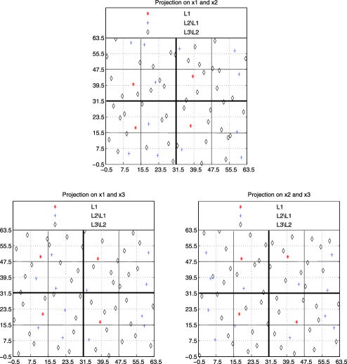
Figure 2: Bivariate projections among $x_{1},x_{2},x_{3}$ of $L_{3}$ in Example 4.

7.2 Generation of SSFDs

Qian and Wu (2009) proposed a method to obtain SSFDs from SOAs. Here we present a more flexible procedure that can use the SOAs constructed in Sections 4–6 to generate a new class of SSFDs. Without loss of generality, consider the SOAs constructed in Theorem 1.

Algorithm 4.

Step 1. Choose the values of $i,j,I$, where $1\leq j\leq i\leq I$. Suppose $A_{I}$ and $(\Gamma^{i}_{1},\ldots,\Gamma^{i}_{(s_{I}/s_{i})^{k}};\rho_{j})$ are constructed in Theorem 1. Relabel the $s_{I}$ levels of $A_{I}$ as $0,\ldots,s_{I}-1$ according to the following two stages: [(ii)]

Use the projection $\rho_{j}$ defined in (8) to divide the $s_{I}$ levels into $s_{j}$ groups

$$\Phi^{j}_{\alpha}=\bigl{\{}\gamma|\rho_{j}(\gamma)=\alpha,\gamma\in F_{I}\bigr{\}}\qquad\mbox{for }\alpha\in F_{j},$$

each of size $q=s_{I}/s_{j}$.

Arbitrarily label the $s_{j}$ groups as groups $1,\ldots,s_{j}$, and label the $q$ levels within the $g$th group as $(g-1)q,(g-1)q+1,\ldots,gq-1$, for $g=1,\ldots,s_{j}$. This relabeling scheme can be denoted by

$$\bigl{\{}\Phi^{j}_{\alpha}|\alpha\in F_{j}\bigr{\}}\longrightarrow\Lambda^{j}=\bigl{\{}\Lambda^{j}_{g}|g=1,\ldots,s_{j}\bigr{\}},$$ (15)

where $\Lambda^{j}_{g}=\{(g-1)q,(g-1)q+1,\ldots,gq-1|q=s_{I}/s_{j}\}$.

Step 2. Let $M$ be the design obtained by relabeling the levels of $A_{I}$, and use $M$ to obtain an OA-based Latin hypercube $S$.

Step 3. Partition $S$ into $(s_{I}/s_{i})^{k}$ subarrays corresponding to $\Gamma^{i}_{1},\ldots,\break\Gamma^{i}_{(s_{I}/s_{i})^{k}}$, that is, $S=(S_{1}^{\prime},\ldots,S_{(s_{I}/s_{i})^{k}}^{\prime})^{\prime}$ with $S_{l}=S([(l-1)s_{i}^{k}+1]\dvtx ls_{i}^{k})$, $l=1,\ldots,(s_{I}/s_{i})^{k}$.

Theorem 8

For $S=(S_{1}^{\prime},\ldots,S_{(s_{I}/s_{i})^{k}}^{\prime})^{\prime}$ constructed in Algorithm 4, $S$ achieves stratification on the $s_{I}\times s_{I}$ grids in any two dimensions, and $S_{l}$ achieves stratification on the $s_{j}\times s_{j}$ grids in any two dimensions for $l=1,\ldots,(s_{I}/s_{i})^{k}$. Thus, $S=(S_{1}^{\prime},\ldots,S_{(s_{I}/s_{i})^{k}}^{\prime})^{\prime}$ is an SSFD with $(s_{I}/s_{i})^{k}$ slices.

By noting that $A_{I}$ and $\rho_{j}(\Gamma^{i}_{l})$ for $l=1,\ldots,(s_{I}/s_{i})^{k}$ are all orthogonal arrays of strength two, and following the relabeling scheme given above, the conclusions hold.

Example 5 ((Example 1 continued)).

(i) For $i=j=1$, we have $q=4,\Phi^{1}_{0}=\{\gamma|\rho_{1}(\gamma)=0,\gamma\in F_{3}\}=\{0,x^{2},x,x^{2}+x\},\Phi^{1}_{1}=\{1,x^{2}+1,x+1,x^{2}+x+1\},\Lambda^{1}_{1}=\{0,1,2,3\}$ and $\Lambda^{1}_{2}=\{4,5,6,7\}$. Arbitrarily relabel the levels of $A_{3}$ in Table 1 according to the scheme given in Step 1 as follows:

$$\bigl{\{}\bigl{\{}0,x^{2},x,x^{2}+x\bigr{\}},\bigl{\{}1,x^{2}+1,x+1,x^{2}+x+1\bigr{\}}\bigr{\}}\longrightarrow\bigl{\{}\{0,1,2,3\},\{4,5,6,7\}\bigr{\}},$$

and then obtain an OA-based Latin hypercube $S$. Let $S_{l}=S([4(l-1)+1]\dvtx 4l),l=1,\ldots,16$. Note that $S$ achieves stratification on the $8\times 8$ grids in any two dimensions, $S_{l}$ achieves stratification on the $2\times 2$ grids in any two dimensions, and $S=(S_{1}^{\prime},\ldots,S_{16}^{\prime})^{\prime}$ is an SSFD with 16 slices.

(ii) For $i=j=2$, we have $q=2,\Phi^{2}_{0}=\{0,x^{2}\},\Phi^{2}_{x}=\{x,x^{2}+x\},\Phi^{2}_{1}=\{1,x^{2}+1\},\Phi^{2}_{x+1}=\{x+1,x^{2}+x+1\},\Lambda^{2}_{1}=\{0,1\},\Lambda^{2}_{2}=\{2,3\},\Lambda^{2}_{3}=\{4,5\}$ and $\Lambda^{2}_{4}=\{6,7\}$. Relabel the levels of $A_{3}$ according to

$$\bigl{\{}\bigl{\{}0,x^{2}\bigr{\}},\bigl{\{}x,x^{2}+x\bigr{\}},\bigl{\{}1,x^{2}+1\bigr{\}},\bigl{\{}x+1,x^{2}+x+1\bigr{\}}\bigr{\}}$$

$$\qquad\longrightarrow\bigl{\{}\{0,1\},\{2,3\},\{4,5\},\{6,7\}\bigr{\}},$$

to obtain an OA-based Latin hypercube $S=(S_{1}^{\prime},\ldots,S_{4}^{\prime})^{\prime}$, where $S_{l}=\break S([16(l-1)+1]\dvtx 16l),l=1,\ldots,4$. Similarly, $S$ achieves stratification on the $8\times 8$ grids in any two dimensions, $S_{l}$ achieves stratification on the $4\times 4$ grids in any two dimensions, and $S=(S_{1}^{\prime},\ldots,S_{4}^{\prime})^{\prime}$ is an SSFD with 4 slices.

Remark 5.

If we relabel the levels of $A_{3}$ according to

$$\bigl{\{}\bigl{\{}0,x^{2}\bigr{\}},\bigl{\{}x,x^{2}+x\bigr{\}}\bigr{\}} \longrightarrow \bigl{\{}\{0,1\},\{2,3\}\bigr{\}}\quad\mbox{and}$$

$$\bigl{\{}\bigl{\{}1,x^{2}+1\bigr{\}},\bigl{\{}x+1,x^{2}+x+1\bigr{\}}\bigr{\}} \longrightarrow \bigl{\{}\{4,5\},\{6,7\}\bigr{\}},$$

in Example 5, then by Theorem 8, we have: [(a)]

$S$ can be partitioned into 16 slices, $S([4(l-1)+1]\dvtx 4l)$ for $l=1,\ldots,16$, each of which achieves stratification on the $2\times 2$ grids in any two dimensions;

$S$ can be partitioned into 4 slices, $S([16(l-1)+1]\dvtx 16l)$ for $l=1,\ldots,4$, each of which achieves stratification on the $4\times 4$ grids in any two dimensions;

$S$ achieves stratification on the $8\times 8$ grids in any two dimensions;

$S$ is an SSFD that can be sliced into 4 or 16 slices. Therefore, under the same relabel scheme (5), $S$ can be used to conduct computer experiments with qualitative factors of 4 and 16 distinct level combinations, respectively. A further discussion on $S$ will be found in Example 6.

Inspired by Remark 5, we now propose a new construction of SSFDs from SOAs which can generate SSFDs with different numbers of slices simultaneously. A new permutation is needed. We call $\pi_{\mathrm{sp}}=(\pi_{\mathrm{sp}}(1),\ldots,\pi_{\mathrm{sp}}(s_{I}))$ a sliced permutation with $I$ layers on $Z_{s_{I}}$, if

$$\bigl{\{}\pi_{\mathrm{sp}}\bigl{(}(g-1)q+1\bigr{)},\pi_{\mathrm{sp}}\bigl{(}(g-1)q+2\bigr{)},\ldots,\pi_{\mathrm{sp}}(gq)\bigr{\}}\in\Lambda^{j}$$

for $j=1,\ldots,I-1$, $g=1,\ldots,s_{j}$ and $q=s_{I}/s_{j}$, where $\Lambda^{j}$ is defined in (15).

Algorithm 5.

Step 1. Suppose $A_{I}$ is constructed in Theorem 1 and $\pi^{l}_{\mathrm{sp}}$ is a sliced permutation with $I$ layers on $Z_{s_{I}}$, $l=1,\ldots,(p^{k}-1)/(p-1)$.

Step 2. Relabel the levels of the $l$th column of $A_{I}$ according to $V_{F_{I}}(r)\longrightarrow\pi^{l}_{\mathrm{sp}}(r)$ for $r=1,\ldots,s_{I}$, and $l=1,\ldots,(p^{k}-1)/(p-1)$, where $V_{F_{I}}=V_{T_{1}}\oplus V_{T_{2}}\oplus\cdots\oplus V_{T_{I}}$ defined in (4). Let $M$ be the resulting matrix.

Step 3. Obtain an OA-based Latin hypercube $S$ from $M$.

Step 4. For $i=1,\ldots,I-1$, partition $S$ into $(s_{I}/s_{i})^{k}$ subarrays with an equal number of rows, that is, $S=((S_{1}^{i})^{\prime},\ldots,(S_{(s_{I}/s_{i})^{k}}^{i})^{\prime})^{\prime}$ with $S_{l}^{i}=S([(l-1)s_{i}^{k}+1]\dvtx ls_{i}^{k})$ for $l=1,\ldots,(s_{I}/s_{i})^{k}$.

Theorem 9

For $S=((S_{1}^{i})^{\prime},\ldots,(S_{(s_{I}/s_{i})^{k}}^{i})^{\prime})^{\prime}$ constructed in Algorithm 5, $S_{l}^{i}$ achieves stratification on the $s_{j}\times s_{j}$ grids in any two dimensions, for $l=1,\ldots,(s_{I}/s_{i})^{k}$ and $1\leq j\leq i\leq I$. Thus, $S=((S_{1}^{i})^{\prime},\ldots,(S_{(s_{I}/s_{i})^{k}}^{i})^{\prime})^{\prime}$ is an SSFD with $(s_{I}/s_{i})^{k}$ slices, for $i=1,\ldots,I-1$.

For any $\alpha\in F_{I}$, let ${\alpha}_{l}$ denote the corresponding element in $\pi^{l}_{\mathrm{sp}}$ under the relabeling $V_{F_{I}}\longrightarrow\pi^{l}_{\mathrm{sp}},l=1,\ldots,(p^{k}-1)/(p-1)$. Since $A_{I}$ and $\rho_{j}(\Gamma^{i}_{l})$ for $l=1,\ldots,(s_{I}/s_{i})^{k}$ and $1\leq j\leq i\leq I-1$ are all orthogonal arrays of strength two, it suffices to prove that for any $\alpha,\beta\in F_{j}$ with $\alpha\neq\beta$, ${\alpha}_{l}$ and ${\beta}_{l}$ fall in different sets defined by $\{0,1,\ldots,q-1\},\{q,q+1,\ldots,2q-1\},\ldots,\{(s_{j}-1)q,(s_{j}-1)q+1,\ldots,s_{j}q-1\}$, where $q=s_{I}/s_{j}$. Note that $V_{F_{I}}=V_{T_{1}}\oplus V_{T_{2}}\oplus\cdots\oplus V_{T_{I}}=V_{F_{j}}\oplus(V_{T_{j+1}}\oplus\cdots\oplus V_{T_{I}})$ and the first element of $V_{T_{i}}$ is 0, $i=1,\ldots,I$, then $\alpha,\beta\in\{V_{F_{I}}(g)|g=1,q+1,2q+1,\ldots,(s_{j}-1)q+1\}$. Suppose $\alpha=V_{F_{I}}(c_{1}q+1),\beta=V_{F_{I}}(c_{2}q+1),c_{1},c_{2}=0,1,\ldots,s_{j}-1$, and $c_{1}\neq c_{2}$. Then ${\alpha}_{l}=\pi^{l}_{\mathrm{sp}}(c_{1}q+1)$ and ${\beta}_{l}=\pi^{l}_{\mathrm{sp}}(c_{2}q+1)$ and, therefore, ${\alpha}_{l}\in\Lambda^{j}_{d_{1}},{\beta}_{l}\in\Lambda^{j}_{d_{2}}$ for some $d_{1},d_{2}=1,2,\ldots,s_{j}$ and $d_{1}\neq d_{2}$ (this is because $|(c_{1}q+1)-(c_{2}q+1)|=|(c_{1}-c_{2})q|\geq q$), and ${\alpha}_{l}$ and ${\beta}_{l}$ fall in different sets defined by $\{0,1,\ldots,q-1\},\{q,q+1,\ldots,2q-1\},\ldots,\{(s_{j}-1)q,(s_{j}-1)q+1,\ldots,s_{j}q-1\}$.

Table 6: The array $M$ in Example 6

Row	$\bolds{x_{1}}$	$\bolds{x_{2}}$	$\bolds{x_{3}}$	Row	$\bolds{x_{1}}$	$\bolds{x_{2}}$	$\bolds{x_{3}}$
1	0	7	0	33	1	7	1
2	0	1	4	34	1	1	5
3	7	7	4	35	6	7	5
4	7	1	0	36	6	1	1
5	0	5	3	37	1	5	2
6	0	2	7	38	1	2	6
7	7	5	7	39	6	5	6
8	7	2	3	40	6	2	2
9	2	7	3	41	3	7	2
10	2	1	7	42	3	1	6
11	5	7	7	43	4	7	6
12	5	1	3	44	4	1	2
13	2	5	0	45	3	5	1
14	2	2	4	46	3	2	5
15	5	5	4	47	4	5	5
16	5	2	0	48	4	2	1
17	0	6	1	49	1	6	0
18	0	0	5	50	1	0	4
19	7	6	5	51	6	6	4
20	7	0	1	52	6	0	0
21	0	4	2	53	1	4	3
22	0	3	6	54	1	3	7
23	7	4	6	55	6	4	7
24	7	3	2	56	6	3	3
25	2	6	2	57	3	6	3
26	2	0	6	58	3	0	7
27	5	6	6	59	4	6	7
28	5	0	2	60	4	0	3
29	2	4	1	61	3	4	0
30	2	3	5	62	3	3	4
31	5	4	5	63	4	4	4
32	5	3	1	64	4	3	0

Example 6 ((Example 1 continued)).

Generate three sliced permutations with three layers $\pi^{1}_{\mathrm{sp}}=(0,1,2,3,7,6,5,4),\pi^{2}_{\mathrm{sp}}=(7,6,5,4,1,0,2,3)$ and $\pi^{3}_{\mathrm{sp}}=(0,1,3,2,4,5,7,6)$ on $Z_{8}$. Note that

$$\bigl{\{}\pi^{l}_{\mathrm{sp}}\bigl{(}r2^{3-j}+1\bigr{)},\ldots,\pi^{l}_{\mathrm{sp}}\bigl{(}(r+1)2^{3-j}\bigr{)}\bigr{\}}\in\Lambda^{j}$$

for $r=0,1,\ldots,2^{j}-1$ and $j=1,2$, where $\Lambda^{1}=\{\{0,1,2,3\},\{4,5,6,7\}\}$ and $\Lambda^{2}=\{\{0,1\},\{2,3\},\{4,5\},\{6,7\}\}$. Relabel the levels of the $l$th column of $A_{3}$ according to $V_{F_{I}}(r)\longrightarrow\pi^{l}_{\mathrm{sp}}(r),r=1,\ldots,8,l=1,2,3$, where $V_{F_{I}}=\{0,x^{2},x,\break x+x^{2},1,x^{2}+1,x+1,x+x^{2}+1\}$. Denote the resulting matrix by $M$ in Table 6, and use $M$ to obtain an OA-based Latin hypercube $S$ given in columns $x_{1},x_{2}$ and $x_{3}$ in Table 8. Note that $S([4^{i}(l-1)+1]\dvtx 4^{i}l)$ achieves stratification on the $2^{i}\times 2^{i}$ grids in any two dimensions for $l=1,2,\ldots,4^{3-i}$ and $i=1,2$; see Figure 3 for an illustration, where for brevity, we only plot the bivariate projections of $S([16(l-1)+1]\dvtx 16l)$ for $l=1,\ldots,4$.

Table 7: $\mathit{OA}(16,2^{3}4^{3},2)$

1	2	3	4	5	6
0	0	0	0	0	0
0	0	0	0	3	3
0	0	0	3	1	2
0	0	0	3	2	1
0	1	1	2	0	2
0	1	1	2	3	1
0	1	1	1	2	3
0	1	1	1	1	0
1	0	1	2	2	0
1	0	1	2	1	3
1	0	1	1	0	1
1	0	1	1	3	2
1	1	0	0	2	2
1	1	0	0	1	1
1	1	0	3	0	3
1	1	0	3	3	0

The design in Table 8 consists of two parts: the SSFD $S$ (columns $x_{1},x_{2},x_{3}$) obtained in Example 6 for arranging quantitative factors, and an $\mathit{OA}(16,2^{3}4^{3})$ with replicate runs (the last six columns) for arranging qualitative factors, where the original $\mathit{OA}(16,2^{3}4^{3})$ is listed in Table 7. Note that $S$ possesses properties: (i) if $S$ is partitioned into 4 slices with 16 runs in each slice, then each slice achieves stratification on the $4\times 4$ grids in any two dimensions; (ii) if $S$ is partitioned into 16 slices with 4 runs in each slice, then each slice achieves stratification on the $2\times 2$ grids in any two dimensions. Therefore, for the design in Table 8, (i) for any level combination of the three two-level qualitative factors, the design points for the quantitative factors achieve stratification on the $4\times 4$ grids in any two dimensions; (ii) for any level combination of the three four-level qualitative factors, the design points for the quantitative factors achieve stratification on the $2\times 2$ grids in any two dimensions; (iii) it possesses good space-filling properties when collapsed over the qualitative factors. Hence, the design in Table 8 is suitable for conducting a computer experiment with three quantitative factors and six qualitative factors, where three of them have 2 levels and another three have 4 levels.

Table 8: Design with qualitative and quantitative factors, where columns $x_{1},x_{2},x_{3}$ are quantitative ones, $x_{4},x_{5},x_{6}$ are 2-level qualitative ones, and $x_{7},x_{8},x_{9}$ are 4-level qualitative ones

Row	$\bolds{x_{1}}$	$\bolds{x_{2}}$	$\bolds{x_{3}}$	$\bolds{x_{4}}$	$\bolds{x_{5}}$	$\bolds{x_{6}}$	$\bolds{x_{7}}$	$\bolds{x_{8}}$	$\bolds{x_{9}}$
1	01	63	03	0	0	0	0	0	0
2	03	13	37	0	0	0	0	0	0
3	60	61	32	0	0	0	0	0	0
4	62	12	00	0	0	0	0	0	0
5	04	47	31	0	0	0	0	3	3
6	00	23	57	0	0	0	0	3	3
7	56	42	62	0	0	0	0	3	3
8	61	17	29	0	0	0	0	3	3
9	18	59	24	0	0	0	3	1	2
10	19	10	63	0	0	0	3	1	2
11	40	57	60	0	0	0	3	1	2
12	42	11	30	0	0	0	3	1	2
13	17	43	07	0	0	0	3	2	1
14	22	20	34	0	0	0	3	2	1
15	46	40	36	0	0	0	3	2	1
16	44	22	06	0	0	0	3	2	1
17	05	51	09	0	1	1	2	0	2
18	02	00	41	0	1	1	2	0	2
19	58	52	42	0	1	1	2	0	2
20	57	04	15	0	1	1	2	0	2
21	06	37	18	0	1	1	2	3	1
22	07	29	54	0	1	1	2	3	1
23	63	34	49	0	1	1	2	3	1
24	59	25	17	0	1	1	2	3	1
25	21	53	21	0	1	1	1	2	3
26	20	06	48	0	1	1	1	2	3
27	41	48	55	0	1	1	1	2	3
28	45	05	23	0	1	1	1	2	3
29	23	36	08	0	1	1	1	1	0
30	16	26	45	0	1	1	1	1	0
31	47	39	43	0	1	1	1	1	0
32	43	24	10	0	1	1	1	1	0
33	09	58	11	1	0	1	2	2	0
34	10	08	40	1	0	1	2	2	0
35	53	56	44	1	0	1	2	2	0
36	54	15	14	1	0	1	2	2	0
37	15	41	22	1	0	1	2	1	3
38	13	21	50	1	0	1	2	1	3
39	48	46	51	1	0	1	2	1	3
40	52	16	16	1	0	1	2	1	3
41	27	62	20	1	0	1	1	0	1
42	30	14	52	1	0	1	1	0	1
43	33	60	53	1	0	1	1	0	1
44	32	09	19	1	0	1	1	0	1

Table 8: (Continued)

Row	$\bolds{x_{1}}$	$\bolds{x_{2}}$	$\bolds{x_{3}}$	$\bolds{x_{4}}$	$\bolds{x_{5}}$	$\bolds{x_{6}}$	$\bolds{x_{7}}$	$\bolds{x_{8}}$	$\bolds{x_{9}}$
45	25	44	13	1	0	1	1	3	2
46	31	19	46	1	0	1	1	3	2
47	37	45	47	1	0	1	1	3	2
48	39	18	12	1	0	1	1	3	2
49	11	49	1	1	1	0	0	2	2
50	08	01	33	1	1	0	0	2	2
51	49	54	38	1	1	0	0	2	2
52	50	07	05	1	1	0	0	2	2
53	14	33	27	1	1	0	0	1	1
54	12	27	61	1	1	0	0	1	1
55	51	32	59	1	1	0	0	1	1
56	55	28	25	1	1	0	0	1	1
57	24	55	26	1	1	0	3	0	3
58	29	02	56	1	1	0	3	0	3
59	34	50	58	1	1	0	3	0	3
60	38	03	28	1	1	0	3	0	3
61	28	38	02	1	1	0	3	3	0
62	26	30	35	1	1	0	3	3	0
63	35	35	39	1	1	0	3	3	0
64	36	31	04	1	1	0	3	3	0

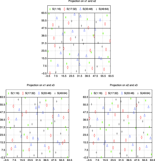
Figure 3: Bivariate projections among $x_{1}$, $x_{2}$ and $x_{3}$ of $S$ in Example 6.

We have provided some new constructions of NSFDs and SSFDs based on NOAs and SOAs of strength two, respectively. Better NSFDs and SSFDs can be obtained by using NOAs and SOAs with strength greater than two. See Remarks 1 and 2, Theorems 3 and 5 and Corollary 2.

8 Comparisons and concluding remarks

The families of NSFDs constructed by the existing methods are limited to two layers, with the exception of Haaland and Qian (2010). The method of Haaland and Qian (2010) is based on the infinite $(t,s)$-sequences which are more difficult to obtain than the orthogonal arrays used in our methods. Here are some comparisons between our methods and the existing constructions.

Qian, Tang and Wu (2009) (QTW) and Qian, Ai and Wu (2009) (QAW) presented several methods for constructing NSFDs with two layers from NOAs and NDMs. NSFDs with more than two layers cannot be constructed by using their methods. The technical reason is that the modulus projection used in Qian, Tang and Wu (2009) cannot be extended to covering more than two layers, as argued in Section 3.2. The subgroup projection presented in this paper is different and more general, and it has been used to generate more NSFDs which can accommodate nesting with an arbitrary number of layers and are more flexible in run size. Qian and Ai (2010) (QA) proposed some construction methods for NOAs and NDMs with two layers based on Galois fields and incomplete pairwise orthogonal Latin squares. Qian (2009) presented a method for constructing nested Latin hypercube designs, but the resulting designs can achieve stratification only in one dimension. Thus, we only present the comparisons among QTW, QAW, QA and our proposed methods (SLQ). The comparison among QAW, QA and SLQ for the construction of NDMs with two layers, and the comparison among QTW, QAW, QA and SLQ for the construction of NOAs with two layers, are listed in Tables 9 and 10, respectively. Since the construction of incomplete pairwise orthogonal Latin squares is still an open problem, thus we only tabulate the results obtained based on Galois fields in QA. In addition, QAW and the present paper presented several indirect methods to obtain NOAs based on existing NOAs or NDMs, for example, Theorems 4, 5 in QAW and Theorem 4 in the present paper. In Tables 9 and 10, we only tabulate the NOAs and NDMs that can be directly constructed. Moreover, Tables 11 and 12 tabulate some construction results of the proposed methods for designs with more than two layers.

Table 9: Comparisons among the $\mathit{NDM}(D_{1},D;\rho_{1},\rho_{2})$’s constructed by QAW, QA and SLQ

Methods		$\bolds{\rho_{1}(D_{1})}$	$\bolds{D}$	Constraintstt9
QAW	I	$D(p^{m},p^{2},p^{m})$	$D(p^{m+1},p^{2},p^{m+1})$	$m\geq 2$
	II	$D(p^{m},p^{2},p^{m})$	$D(p^{m+2},p^{2},p^{m+2})$	$p=2,3$
	III	$D(p^{m+1},p^{3},p^{m})$	$D(p^{m+2},p^{3},p^{m+2})$
	IV	$D(p^{m+1},p^{3},p^{m})$	$D(p^{m+3},p^{3},p^{m+3})$
	V	$D(p^{m+2},p^{4},p^{m})$	$D(p^{m+3},p^{4},p^{m+3})$
QA		$D(p^{u_{1}},p^{u_{1}},p^{u_{1}})$	$D(p^{u_{2}},p^{u_{1}},p^{u_{2}})$	$u_{1}<u_{2},u_{1}|u_{2}$
SLQ	Theorem 4	$D(lp^{u_{2}},p^{u_{1}},p^{u_{2}})$	$D(p^{u_{3}},p^{u_{1}},p^{u_{3}})$	$u_{i}|u_{i+1},i=1,2$,
				$u_{2}<u_{3}$, $l<p^{u_{3}-u_{2}}$
	Theorem 6	$D(lr_{1},c,p^{u_{1}})$	$D(r_{1}r_{2},c,p^{u_{1}+u_{2}})$	$D(r_{i},c,p^{u_{i}})$ exists,
				$i=1,2$, $l<r_{2}$

[*]tt9$p$ is any prime number.

Table 10: Comparisons among the $\mathit{NOA}(A_{1},A;\rho_{1},\rho_{2})$’s constructed by QTW, QAW, QA and SLQ

Methods		$\bolds{\rho_{1}(A_{1})}$	$\bolds{A}$	Constraintstt10
QTW		$\mathit{OA}(p^{ku_{1}},\frac{p^{ku_{1}}-1}{p^{u_{1}}-1},p^{u_{1}},2)$	$\mathit{OA}(p^{ku_{2}},\frac{p^{ku_{1}}-1}{p^{u_{1}}-1},p^{u_{2}},2)$	$2u_{1}\leq u_{2}+1$
QAW		$\mathit{OA}(s^{2}_{1},3,s_{1},2)$	$\mathit{OA}(s^{2}_{2},3,s_{2},2)$	$s_{1}<s_{2},s_{1}|s_{2}$
QA	I	$\mathit{OA}(p^{ku_{1}},\frac{p^{ku_{1}}-1}{p^{u_{1}}-1},p^{u_{1}},2)$	$\mathit{OA}(p^{ku_{2}},\frac{p^{ku_{1}}-1}{p^{u_{1}}-1},p^{u_{2}},2)$	$u_{1}<u_{2},u_{1}|u_{2}$
	II	$\mathit{OA}(p^{ku_{1}},p^{u_{1}}+1,p^{u_{1}},k)$	$\mathit{OA}(p^{ku_{2}},p^{u_{1}}+1,p^{u_{2}},k)$	$u_{1}<u_{2}$, $u_{1}|u_{2}$,
				$p^{u_{1}}\geq k-1$
SLQ	Theorem 1	$\mathit{OA}(lp^{ku_{1}},\frac{p^{k}-1}{p-1},p^{u_{1}},2)$	$\mathit{OA}(p^{ku_{2}},\frac{p^{k}-1}{p-1},p^{u_{2}},2)$	$l<p^{k(u_{2}-u_{1})}$,
				$u_{1}<u_{2}$
	Theorem 2	$\mathit{OA}(lp^{ku_{1}},\frac{p^{ku_{1}}-1}{p^{u_{1}}-1},p^{u_{1}},2)$	$\mathit{OA}(p^{ku_{2}},\frac{p^{ku_{1}}-1}{p^{u_{1}}-1},p^{u_{2}},2)$	$l<p^{k(u_{2}-u_{1})}$,
				$u_{1}<u_{2},u_{1}|u_{2}$
	Theorem 3	$\mathit{OA}(lp^{ku_{1}},p^{u_{1}}+1,p^{u_{1}},k)$	$\mathit{OA}(p^{ku_{2}},p^{u_{1}}+1,p^{u_{2}},k)$	$l<p^{k(u_{2}-u_{1})},u_{1}<u_{2}$,
				$u_{1}|u_{2}$, $p^{u_{1}}\geq k-1$
	Theorem 5	$\mathit{OA}(ln_{1},m,p^{u_{1}},t)$	$\mathit{OA}(n_{1}n_{2},m,p^{u_{1}+u_{2}},t)$	$\mathit{OA}(n_{i},m,p^{u_{i}},t)$ exists,
				$i=1,2$, $l<n_{2}$

[*]tt10$p$ is any prime number.

Table 11: The $\mathit{NDM}(D_{1},\ldots,D_{I};\rho_{1},\ldots,\rho_{I})$’s constructed in this paper for $I>2$

Methods	$\bolds{\rho_{i}(D_{i}),\ i=1,\ldots,I}$	Constraintstt11
Theorem 4	$D(p^{u_{i}},p^{u_{1}},p^{u_{i}})$	$u_{i}<u_{i+1}$, $u_{i}|u_{i+1},i=1,\ldots,I-1$
Theorem 6	$D(\prod^{i}_{l=1}r_{l},c,p^{\sum^{i}_{l=1}u_{l}})$	$D(r_{i},c,p^{u_{i}})$ exists, $i=1,\ldots,I$

[*]tt11$p$ is any prime number.

Table 12: The $\mathit{NOA}(A_{1},\ldots,A_{I};\rho_{1},\ldots,\rho_{I})$’s constructed in this paper for $I>2$

Methods	$\bolds{\rho_{i}(A_{i}),\ i=1,\ldots,I}$	Constraintstt12
Theorem 1	$\mathit{OA}(p^{ku_{i}},\frac{p^{k}-1}{p-1},p^{u_{i}},2)$	$u_{i}<u_{i+1},i=1,\ldots,I-1$
Theorem 2	$\mathit{OA}(p^{ku_{i}},\frac{p^{ku_{1}}-1}{p^{u_{1}}-1},p^{u_{i}},2)$	$u_{i}<u_{i+1},u_{i}|u_{i+1},i=1,\ldots,I-1$
Theorem 3	$\mathit{OA}(p^{ku_{i}},p^{u_{1}}+1,p^{u_{i}},k)$	$p^{u_{1}}\geq k-1$, $u_{i}<u_{i+1}$,
		$u_{i}|u_{i+1},i=1,\ldots,I-1$
Corollary 2	$\mathit{OA}(\prod^{i}_{l=1}n_{l},m,p^{\sum^{i}_{l=1}u_{l}},t)$	$\mathit{OA}(n_{i},m,p^{u_{i}},t)$ exists, $i=1,\ldots,I$

[*]tt12$p$ is any prime number.

From these tables and our construction methods, we can see that: [(iii)]

The proposed methods have more flexible choices of the parameters, and thus can generate much more new NDMs and NOAs, hence much more new NSFDs.

For NSFDs with two layers, some of the construction results of QTW, QAW and QA can also be obtained by the proposed methods. For example, in Table 9, by taking $l=1,p=2,3,u_{1}=m,u_{2}=2,r_{1}=p^{m}$, and $r_{2}=c=p^{2}$, then the NDMs obtained by our Theorem 6 are just those constructed by II of QAW. In addition, most of the NOAs and NDMs obtained by the proposed methods have no overlap with that of QTW, QAW and QA.

The proposed methods can generate various NDMs and NOAs with more than two layers; see Tables 11 and 12.

Moreover, the methods for obtaining NOAs can also be used to generate SOAs after some suitable modifications, which are useful for constructing SSFDs for computer experiments with both qualitative and quantitative factors [Qian and Wu (2009)].

The newly proposed methods are easy to implement. The generated NSFDs and SSFDs can be used not only in computer experiments, but also in many other fields as mentioned in Section 1.

References

- Bose and Bush (1952) {barticle}[mr] \bauthor\bsnmBose, \bfnmR. C.\binitsR. C. and \bauthor\bsnmBush, \bfnmK. A.\binitsK. A. (\byear1952). \btitleOrthogonal arrays of strength two and three. \bjournalAnn. Math. Statistics \bvolume23 \bpages508–524. \bidissn=0003-4851, mr=0051204 \bptokimsref\endbibitem
- Choi et al. (2008) {barticle}[auto:STB—2014/05/26—13:19:10] \bauthor\bsnmChoi, \bfnmS.\binitsS., \bauthor\bsnmAlonso, \bfnmJ. J.\binitsJ. J., \bauthor\bsnmKroo, \bfnmI. M.\binitsI. M. and \bauthor\bsnmWintzer, \bfnmM.\binitsM. (\byear2008). \btitleMultifidelity design optimization of low-boom supersonic jets. \bjournalJournal of Aircraft \bvolume45 \bpages106–118. \bptokimsref\endbibitem
- Dewettinck et al. (1999) {barticle}[auto:STB—2014/05/26—13:19:10] \bauthor\bsnmDewettinck, \bfnmK.\binitsK., \bauthor\bsnmVisscher, \bfnmA. D.\binitsA. D., \bauthor\bsnmDeroo, \bfnmL.\binitsL. and \bauthor\bsnmHuyghebaert, \bfnmA.\binitsA. (\byear1999). \btitleModeling the steady-state thermodynamic operation point of top-spray fluidized bed processing. \bjournalJournal of Food Engineering \bvolume39 \bpages131–143. \bptokimsref\endbibitem
- Fang, Li and Sudjianto (2006) {bbook}[mr] \bauthor\bsnmFang, \bfnmKai-Tai\binitsK.-T., \bauthor\bsnmLi, \bfnmRunze\binitsR. and \bauthor\bsnmSudjianto, \bfnmAgus\binitsA. (\byear2006). \btitleDesign and Modeling for Computer Experiments. \bpublisherChapman & Hall/CRC, \blocationBoca Raton, FL. \bidmr=2223960 \bptnotecheck year \bptokimsref\endbibitem
- Fasshauer (2007) {bbook}[mr] \bauthor\bsnmFasshauer, \bfnmGregory E.\binitsG. E. (\byear2007). \btitleMeshfree Approximation Methods with MATLAB. \bseriesInterdisciplinary Mathematical Sciences \bvolume6. \bpublisherWorld Scientific, \blocationHackensack, NJ. \bidmr=2357267 \bptokimsref\endbibitem
- Floater and Iske (1996) {barticle}[mr] \bauthor\bsnmFloater, \bfnmMichael S.\binitsM. S. and \bauthor\bsnmIske, \bfnmArmin\binitsA. (\byear1996). \btitleMultistep scattered data interpolation using compactly supported radial basis functions. \bjournalJ. Comput. Appl. Math. \bvolume73 \bpages65–78. \biddoi=10.1016/0377-0427(96)00035-0, issn=0377-0427, mr=1424869 \bptokimsref\endbibitem
- Haaland and Qian (2010) {barticle}[mr] \bauthor\bsnmHaaland, \bfnmBen\binitsB. and \bauthor\bsnmQian, \bfnmPeter Z. G.\binitsP. Z. G. (\byear2010). \btitleAn approach to constructing nested space-filling designs for multi-fidelity computer experiments. \bjournalStatist. Sinica \bvolume20 \bpages1063–1075. \bidissn=1017-0405, mr=2729853 \bptokimsref\endbibitem
- Haaland and Qian (2011) {barticle}[mr] \bauthor\bsnmHaaland, \bfnmBen\binitsB. and \bauthor\bsnmQian, \bfnmPeter Z. G.\binitsP. Z. G. (\byear2011). \btitleAccurate emulators for large-scale computer experiments. \bjournalAnn. Statist. \bvolume39 \bpages2974–3002. \biddoi=10.1214/11-AOS929, issn=0090-5364, mr=3012398 \bptokimsref\endbibitem
- Han et al. (2009) {barticle}[mr] \bauthor\bsnmHan, \bfnmGang\binitsG., \bauthor\bsnmSantner, \bfnmThomas J.\binitsT. J., \bauthor\bsnmNotz, \bfnmWilliam I.\binitsW. I. and \bauthor\bsnmBartel, \bfnmDonald L.\binitsD. L. (\byear2009). \btitlePrediction for computer experiments having quantitative and qualitative input variables. \bjournalTechnometrics \bvolume51 \bpages278–288. \biddoi=10.1198/tech.2009.07132, issn=0040-1706, mr=2751072 \bptokimsref\endbibitem
- Hedayat, Sloane and Stufken (1999) {bbook}[mr] \bauthor\bsnmHedayat, \bfnmA. S.\binitsA. S., \bauthor\bsnmSloane, \bfnmN. J. A.\binitsN. J. A. and \bauthor\bsnmStufken, \bfnmJohn\binitsJ. (\byear1999). \btitleOrthogonal Arrays: Theory and Applications. \bpublisherSpringer, \blocationNew York. \biddoi=10.1007/978-1-4612-1478-6, mr=1693498 \bptokimsref\endbibitem
- Herstein (1996) {bbook}[mr] \bauthor\bsnmHerstein, \bfnmI. N.\binitsI. N. (\byear1996). \btitleAbstract Algebra, \bedition3rd ed. \bpublisherPrentice Hall, \blocationUpper Saddle River, NJ. \bidmr=1375019 \bptokimsref\endbibitem
- Husslage et al. (2003) {barticle}[auto:STB—2014/05/26—13:19:10] \bauthor\bsnmHusslage, \bfnmB.\binitsB., \bauthor\bsnmDam, \bfnmE. V.\binitsE. V., \bauthor\bsnmHertog, \bfnmD. D.\binitsD. D., \bauthor\bsnmStehouwer, \bfnmP.\binitsP. and \bauthor\bsnmStinstra, \bfnmE.\binitsE. (\byear2003). \btitleCollaborative metamodeling: Coordinating simulation-based product design. \bjournalConcurrent Eng. \bvolume11 \bpages267–278. \bptokimsref\endbibitem
- McKay, Beckman and Conover (1979) {barticle}[mr] \bauthor\bsnmMcKay, \bfnmM. D.\binitsM. D., \bauthor\bsnmBeckman, \bfnmR. J.\binitsR. J. and \bauthor\bsnmConover, \bfnmW. J.\binitsW. J. (\byear1979). \btitleA comparison of three methods for selecting values of input variables in the analysis of output from a computer code. \bjournalTechnometrics \bvolume21 \bpages239–245. \biddoi=10.2307/1268522, issn=0040-1706, mr=0533252 \bptokimsref\endbibitem
- Molina-Cristóbal et al. (2010) {bmisc}[auto:STB—2014/05/26—13:19:10] \bauthor\bsnmMolina-Cristóbal, \bfnmA.\binitsA., \bauthor\bsnmPalmer, \bfnmP. R.\binitsP. R., \bauthor\bsnmSkinner, \bfnmB. A.\binitsB. A. and \bauthor\bsnmParks, \bfnmG. T.\binitsG. T. (\byear2010). \bhowpublishedMulti-fidelity simulation modelling in optimization of a submarine propulsion system. In Proceedings of the 2010 IEEE Vehicle Power and Propulsion Conference (VPPC). Lille, France. \bptokimsref\endbibitem
- Mukerjee, Qian and Jeff Wu (2008) {barticle}[mr] \bauthor\bsnmMukerjee, \bfnmRahul\binitsR., \bauthor\bsnmQian, \bfnmPeter Z. G.\binitsP. Z. G. and \bauthor\bsnmJeff Wu, \bfnmC. F.\binitsC. F. (\byear2008). \btitleOn the existence of nested orthogonal arrays. \bjournalDiscrete Math. \bvolume308 \bpages4635–4642. \biddoi=10.1016/j.disc.2007.08.096, issn=0012-365X, mr=2438169 \bptokimsref\endbibitem
- Qian (2009) {barticle}[mr] \bauthor\bsnmQian, \bfnmPeter Z. G.\binitsP. Z. G. (\byear2009). \btitleNested Latin hypercube designs. \bjournalBiometrika \bvolume96 \bpages957–970. \biddoi=10.1093/biomet/asp045, issn=0006-3444, mr=2767281 \bptokimsref\endbibitem
- Qian (2012) {barticle}[mr] \bauthor\bsnmQian, \bfnmPeter Z. G.\binitsP. Z. G. (\byear2012). \btitleSliced Latin hypercube designs. \bjournalJ. Amer. Statist. Assoc. \bvolume107 \bpages393–399. \biddoi=10.1080/01621459.2011.644132, issn=0162-1459, mr=2949368 \bptokimsref\endbibitem
- Qian and Ai (2010) {barticle}[mr] \bauthor\bsnmQian, \bfnmPeter Z. G.\binitsP. Z. G. and \bauthor\bsnmAi, \bfnmMingyao\binitsM. (\byear2010). \btitleNested lattice sampling: A new sampling scheme derived by randomizing nested orthogonal arrays. \bjournalJ. Amer. Statist. Assoc. \bvolume105 \bpages1147–1155. \biddoi=10.1198/jasa.2010.tm09365, issn=0162-1459, mr=2752610 \bptokimsref\endbibitem
- Qian, Ai and Wu (2009) {barticle}[mr] \bauthor\bsnmQian, \bfnmPeter Z. G.\binitsP. Z. G., \bauthor\bsnmAi, \bfnmMingyao\binitsM. and \bauthor\bsnmWu, \bfnmC. F. Jeff\binitsC. F. J. (\byear2009). \btitleConstruction of nested space-filling designs. \bjournalAnn. Statist. \bvolume37 \bpages3616–3643. \biddoi=10.1214/09-AOS690, issn=0090-5364, mr=2549572 \bptokimsref\endbibitem
- Qian, Tang and Wu (2009) {barticle}[mr] \bauthor\bsnmQian, \bfnmPeter Z. G.\binitsP. Z. G., \bauthor\bsnmTang, \bfnmBoxin\binitsB. and \bauthor\bsnmWu, \bfnmC. F. Jeff\binitsC. F. J. (\byear2009). \btitleNested space-filling designs for computer experiments with two levels of accuracy. \bjournalStatist. Sinica \bvolume19 \bpages287–300. \bidissn=1017-0405, mr=2487890 \bptokimsref\endbibitem
- Qian and Wu (2009) {barticle}[mr] \bauthor\bsnmQian, \bfnmPeter Z. G.\binitsP. Z. G. and \bauthor\bsnmWu, \bfnmC. F. Jeff\binitsC. F. J. (\byear2009). \btitleSliced space-filling designs. \bjournalBiometrika \bvolume96 \bpages945–956. \biddoi=10.1093/biomet/asp044, issn=0006-3444, mr=2767280 \bptokimsref\endbibitem
- Qian, Wu and Wu (2008) {barticle}[mr] \bauthor\bsnmQian, \bfnmPeter Z. G.\binitsP. Z. G., \bauthor\bsnmWu, \bfnmHuaiqing\binitsH. and \bauthor\bsnmWu, \bfnmC. F. Jeff\binitsC. F. J. (\byear2008). \btitleGaussian process models for computer experiments with qualitative and quantitative factors. \bjournalTechnometrics \bvolume50 \bpages383–396. \biddoi=10.1198/004017008000000262, issn=0040-1706, mr=2457574 \bptokimsref\endbibitem
- Santner, Williams and Notz (2003) {bbook}[mr] \bauthor\bsnmSantner, \bfnmThomas J.\binitsT. J., \bauthor\bsnmWilliams, \bfnmBrian J.\binitsB. J. and \bauthor\bsnmNotz, \bfnmWilliam I.\binitsW. I. (\byear2003). \btitleThe Design and Analysis of Computer Experiments. \bpublisherSpringer, \blocationNew York. \biddoi=10.1007/978-1-4757-3799-8, mr=2160708 \bptokimsref\endbibitem
- Schmidt, Cruz and Iyengar (2005) {barticle}[auto:STB—2014/05/26—13:19:10] \bauthor\bsnmSchmidt, \bfnmR. R.\binitsR. R., \bauthor\bsnmCruz, \bfnmE. E.\binitsE. E. and \bauthor\bsnmIyengar, \bfnmM. K.\binitsM. K. (\byear2005). \btitleChallenges of data center thermal management. \bjournalIBM Journal of Research and Development \bvolume49 \bpages709–723. \bptokimsref\endbibitem
- Tang (1993) {barticle}[mr] \bauthor\bsnmTang, \bfnmBoxin\binitsB. (\byear1993). \btitleOrthogonal array-based Latin hypercubes. \bjournalJ. Amer. Statist. Assoc. \bvolume88 \bpages1392–1397. \bidissn=0162-1459, mr=1245375 \bptokimsref\endbibitem
- Williams, Morris and Santner (2009) {bmisc}[auto:STB—2014/05/26—13:19:10] \bauthor\bsnmWilliams, \bfnmB.\binitsB., \bauthor\bsnmMorris, \bfnmM.\binitsM. and \bauthor\bsnmSantner, \bfnmT.\binitsT. (\byear2009). \bhowpublishedUsing multiple computer models/multiple data sources simultaneously to infer calibration parameters. Paper presented at the 2009 INFORMS Annual Conference, October 11–14, San Diego, CA. \bptokimsref\endbibitem
- Xu, Haaland and Qian (2011) {barticle}[mr] \bauthor\bsnmXu, \bfnmXu\binitsX., \bauthor\bsnmHaaland, \bfnmBen\binitsB. and \bauthor\bsnmQian, \bfnmPeter Z. G.\binitsP. Z. G. (\byear2011). \btitleSudoku-based space-filling designs. \bjournalBiometrika \bvolume98 \bpages711–720. \biddoi=10.1093/biomet/asr024, issn=0006-3444, mr=2836416 \bptokimsref\endbibitem
- Zhou, Qian and Zhou (2011) {barticle}[mr] \bauthor\bsnmZhou, \bfnmQiang\binitsQ., \bauthor\bsnmQian, \bfnmPeter Z. G.\binitsP. Z. G. and \bauthor\bsnmZhou, \bfnmShiyu\binitsS. (\byear2011). \btitleA simple approach to emulation for computer models with qualitative and quantitative factors. \bjournalTechnometrics \bvolume53 \bpages266–273. \biddoi=10.1198/TECH.2011.10025, issn=0040-1706, mr=2857704 \bptokimsref\endbibitem