Self-adjoint Dirac type Hamiltonians in one space dimension with a mass jump.

Abstract

Physical self-adjoint extensions and their spectra of the one-dimensional Dirac type Hamiltonian operator in which both the mass and velocity are constant except for a finite jump at one point of the real axis are correctly found. Different boundary conditions on envelope wave functions are studied, and the limiting case of equal masses (with no mass jump) is reviewed. Transport across one-dimensional heterostructures described by the Dirac equation is considered.

Keywords: Self-adjoint extensions, Boundary conditions, Mass jump, Heterostructures, Graphene.

1 Introduction

The discovery of graphene ended the belief that the Dirac equation useless in condensed matter physics [1, 2]. The scientific and technological potential for exploiting charge carriers and quasiparticles with relativistic behavior in tunable condensed matter and atomic physics systems is attracting much attention [3, 4, 5, 6]. In this regard, an important question, as yet only partly explored, remains whether quasi - one dimensional graphene systems support exclusively Dirac - Weyl massless or constant - mass Dirac fermions, or they can induce relativistic quantum field behaviors that require the consideration of position - dependent mass term [7]. The mass jump case was firstly consider in [8] for the spherical defects in the $III-V$ semiconductors and then in [9, 10, 11] for cylindrically symmetric defects in graphene, where the presence of the mass jump was traced back to the graphene sublattice symmetry violation, which is natural but for a short range defect. Using the Dirac - Weyl equation, the break - down of the sublattice symmetry (the equivalence of the two triangular lattices in graphene) can be described in terms of the effective mass that can be position - dependent. The existence of localized Dirac fermions in graphene with inhomogeneous effective mass was considered in [12], where the conditions under which the Dirac fermions are confined are found.

Models with an abrupt discontinuity of the mass and velocity at one point can be used for describing the behavior of a quantum particle moving between two different materials, i.e. an electron moving in a media formed up by two different materials. In each material the particle behaves as if it had a different mass and velocity. The discontinuity point represents the junction between these two materials.

We propose a simple model that describes an electron moving in a media formed up by two different materials given by a one - dimensional system in which the mass and velocity are constant except for a finite jump at one point of the real axis, which is chosen to be the origin for simplicity,

$$m(x)=\begin{cases}m_{l}&\textrm{if}\hskip 5.69046ptx<0\\ m_{r}&\textrm{if}\hskip 5.69046ptx>0,\end{cases}$$ (1)

where $m_{l}$ and $m_{r}$ ($m_{l}\neq m_{r}$) are the masses at rest on the left and right, respectively. In this case, the Hamiltonian operator has the functional form

$$H=\begin{cases}-iv_{l}\sigma_{x}\frac{d}{dx}+m_{l}v^{2}_{l}\sigma_{z}&\textrm{if}\hskip 5.69046ptx<0\\[5.69046pt] -iv_{r}\sigma_{x}\frac{d}{dx}+m_{r}v^{2}_{r}\sigma_{z}&\textrm{if}\hskip 5.69046ptx>0,\end{cases}$$ (2)

where $v_{l},\,v_{r}$ are the Fermi velocities in each medium and

$$\sigma_{x}=\begin{pmatrix}0&1\\ 1&0\end{pmatrix},\;\;\sigma_{z}=\begin{pmatrix}1&0\\ 0&-1\end{pmatrix}$$ (3)

are the Pauli matrices.

The finding appropriate of the boundary conditions in this kind of models is very important to describe the correct physics. The study of the role of the boundary conditions of quantum systems has became a recent focus of activity in different branches of physics [13, 14]. Some examples of quantum physical phenomena which are intimately related to boundary conditions are the Casimir effect [15], the role of edge states [16] and the quantization of conductivity in the Hall effect [17].

In this paper, we show that the operator (2), in a suitable domain, has infinite self-adjoint extensions. All the self-adjoint extensions have real discrete spectrum. Thus, all self-adjoint extensions describe bound states only, but not all the extensions are physically acceptable. We examine which extensions could to play an interesting role according to physical arguments.

The paper is organised as follows: In section 2, we find the set of all possible self-adjoint extensions of $H$. In section 3, we calculate the reflection and transmission coefficients for all self-adjoint extensions, and we use constraints from physical arguments to reduce the set of all possible self-adjoint extensions. From the equation of the poles of the scattering coefficients, we obtain the spectrum that characterizes each self-adjoint extensions.

2 Self - adjoint extensions of H

We will follow to Reed [18] and Naimark [19] to construct the self-adjoint extensions of $H$. To construct the self-adjoint extensions of the operator $H$ we must begin by defining the smaller domain where the action operator makes sense. In this section we will assume that the operator $H$ is densely defined. The domain of the operator $H$, $\mathcal{D}(H)$, is

$$\mathcal{D}(H)=\left\{\psi\in W^{2,1}(\mathbb{R})\otimes\mathbb{C}^{2}\,,\,\psi(0^{-})=\psi(0^{+})=0\right\},$$ (4)

where $W^{2,1}(\mathbb{R})$ is the corresponding Sobolev space, and $\psi$ is a two - component spinor wave function

$$\psi(x)=\begin{pmatrix}\psi_{a}(x)\\ \psi_{b}(x)\end{pmatrix}$$ (5)

The operator $H$ is symmetric and closed. Let $H^{{\dagger}}$ the adjoint of $H$, with domain

$$\mathcal{D}(H^{\dagger})=\left\{\psi\in W^{2,1}(\mathbb{R}\backslash\left\{0\right\})\otimes\mathbb{C}^{2}\right\}.$$ (6)

Note that $\mathcal{D}(H)\subset\mathcal{D}(H^{{\dagger}})$. The deficiency subspaces of $H$ are given by

$$\mathcal{N}_{\pm}=\left\{\psi_{\pm}\in\mathcal{D}(H^{\dagger})\,,\,H^{\dagger}\psi_{\pm}=\pm i\psi_{\pm}\right\},$$ (7)

with the respective dimensions $n_{+}$ and $n_{-}$. These are called the deficiency indices of the operator $H$ and will be denoted by the ordered pair $(n_{+},n_{-})$. The normalized solutions of $H^{\dagger}\psi_{\pm}=\pm i\psi_{\pm}$ are

$$\psi_{+}^{(+)}(x) = \left[\tfrac{(1+m_{r}^{2}v_{r}^{4})}{v_{r}^{2}}\right]^{1/4}\begin{pmatrix}1\\ i\tfrac{\sqrt{1+m_{r}^{2}v_{r}^{4}}}{i+m_{r}v_{r}^{2}}\end{pmatrix}\theta(x)\,e^{-\tfrac{\sqrt{1+m_{r}^{2}v_{r}^{4}}}{v_{r}}x},$$ (8a)

$$\psi_{+}^{(-)}(x) = \left[\tfrac{(1+m_{l}^{2}v_{l}^{4})}{v_{l}^{2}}\right]^{1/4}\begin{pmatrix}1\\ -i\tfrac{\sqrt{1+m_{l}^{2}v_{l}^{4}}}{i+m_{l}v_{l}^{2}}\end{pmatrix}\theta(-x)\,e^{\tfrac{\sqrt{1+m_{l}^{2}v_{l}^{4}}}{v_{l}}x},$$ (8b)

$$\psi_{-}^{(+)}(x) = \left[\tfrac{(1+m_{r}^{2}v_{r}^{4})}{v_{r}^{2}}\right]^{1/4}\begin{pmatrix}1\\ i\tfrac{\sqrt{1+m_{r}^{2}v_{r}^{4}}}{m_{r}v_{r}^{2}-i}\end{pmatrix}\theta(x)\,e^{-\tfrac{\sqrt{1+m_{r}^{2}v_{r}^{4}}}{v_{r}}x},$$ (8c)

$$\psi_{-}^{(-)}(x) = \left[\tfrac{(1+m_{l}^{2}v_{l}^{4})}{v_{l}^{2}}\right]^{1/4}\begin{pmatrix}1\\ -i\tfrac{\sqrt{1+m_{l}^{2}v_{l}^{4}}}{m_{l}v_{l}^{2}-i}\end{pmatrix}\theta(-x)\,e^{\tfrac{\sqrt{1+m_{l}^{2}v_{l}^{4}}}{v_{l}}x},$$ (8d)

where $\theta(x)$ represents the Heaviside step function. Since all the solutions of equations $H^{\dagger}\psi_{\pm}=\pm i\psi_{\pm}$ belong to $L^{2}(\mathbb{R})\otimes\mathbb{C}^{2}$, the deficiency indices are $(2,2)$ and, the according to Naimark [19], every self-adjoint extensions are parametrized by a $U(2)$ matrix. This matrix defines a unique self-adjoint extension, $H_{U}$, of $H$ with domain characterized by means the set of all functions $\phi\in\mathcal{D}(H^{\dagger})$ which satisfy the conditions

$$\begin{pmatrix}\bar{\psi}_{a2}(0^{-})&\bar{\psi}_{a1}(0^{-})\\ \bar{\psi}_{b2}(0^{-})&\bar{\psi}_{b1}(0^{-})\end{pmatrix}\begin{pmatrix}\phi_{a}(0^{-})\\ \phi_{b}(0^{-})\end{pmatrix}=\frac{v_{r}}{v_{l}}\begin{pmatrix}\bar{\psi}_{a2}(0^{+})&\bar{\psi}_{a1}(0^{+})\\ \bar{\psi}_{b2}(0^{+})&\bar{\psi}_{b1}(0^{+})\end{pmatrix}\begin{pmatrix}\phi_{a}(0^{+})\\ \phi_{b}(0^{+})\end{pmatrix}$$ (9)

where $\psi(0^{\pm})\equiv\lim\limits_{x\rightarrow 0^{\pm}}\psi(x)$ and $\phi(0^{\pm})\equiv\lim\limits_{x\rightarrow 0^{\pm}}\phi(x)$, and

$$\psi_{1}(x) =\psi_{+}^{(+)}(x)+U_{11}\psi_{-}^{(+)}(x)+U_{21}\psi_{-}^{(-)}(x)$$ (10)

$$\psi_{2}(x) =\psi_{+}^{(-)}(x)+U_{12}\psi_{-}^{(+)}(x)+U_{22}\psi_{-}^{(-)}(x)$$ (11)

where $\psi_{1}(x),\psi_{2}(x)\in\mathcal{D}(H_{U})$, and $U_{11},U_{12},U_{21},U_{22}$ are complex numbers that determine $U$. The expression (9) can be written in the form

$$\begin{pmatrix}\phi_{a}(0^{+})\\ \phi_{b}(0^{+})\end{pmatrix}=\mathbb{T}\begin{pmatrix}\phi_{a}(0^{-})\\ \phi_{b}(0^{-})\end{pmatrix},$$ (12)

where the $n_{+}\times n_{-}\;$ matrix $\mathbb{T}$ is given by

$$\mathbb{T}=\frac{v_{l}}{v_{r}}\begin{pmatrix}\bar{\psi}_{a2}(0^{+})&\bar{\psi}_{a1}(0^{+})\\ \bar{\psi}_{b2}(0^{+})&\bar{\psi}_{b1}(0^{+})\end{pmatrix}^{-1}\begin{pmatrix}\bar{\psi}_{a2}(0^{-})&\bar{\psi}_{a1}(0^{-})\\ \bar{\psi}_{b2}(0^{-})&\bar{\psi}_{b1}(0^{-})\end{pmatrix},$$ (13)

whose determinat is given by

$$\left|\det\mathbb{T}\right|=\frac{v_{l}}{v_{r}}.$$ (14)

The matrix $\mathbb{T}$ gives the matching conditions at the origin. From (10), we can rewrite the matrix $\mathbb{T}$ in the form

$$\mathbb{T}=\frac{\sqrt{v_{l}}}{2\bar{U}_{12}\sqrt{v_{r}}}\begin{pmatrix}T_{11}&T_{12}\\ T_{21}&T_{22}\end{pmatrix}$$ (15)

with

$$T_{11}= \frac{(1+m_{r}^{2}v_{r}^{4})^{\frac{1}{4}}((1-im_{l}v_{l}^{2})(1+\bar{U}_{11})-(1+im_{l}v_{l}^{2})(\bar{U}_{22}+\det(\bar{U})))}{(1+m_{l}^{2}v_{l}^{4})^{\frac{1}{4}}}$$ (16a)

$$T_{12}= -(1+\det(\bar{U})+\bar{U}_{11}+\bar{U}_{22})((1+m_{l}^{2}v_{l}^{4})(1+m_{r}^{2}v_{r}^{4}))^{\frac{1}{4}}$$ (16b)

$$T_{21}= \frac{(i+m_{l}v_{l}^{2}+\bar{U}_{22}(m_{l}v_{l}^{2}-i))(\bar{U}_{11}(m_{r}v_{r}^{2}-i)+m_{r}v_{r}^{2}+i)}{((1+m_{l}^{2}v_{l}^{4})(1+m_{r}^{2}v_{r}^{4}))^{\frac{1}{4}}}$$ (16c)

$$-\frac{\bar{U}_{12}\bar{U}_{21}(m_{l}v_{l}^{2}-i)(m_{r}v_{r}^{2}-i)}{((1+m_{l}^{2}v_{l}^{4})(1+m_{r}^{2}v_{r}^{4}))^{\frac{1}{4}}}$$

$$T_{22}= \frac{(1+m_{l}^{2}v_{l}^{4})^{\frac{1}{4}}((1-im_{r}v_{r}^{2})(1+\bar{U}_{22})-(1+im_{r}v_{r}^{2})(\bar{U}_{11}+\det(\bar{U})))}{(1+m_{r}^{2}v_{r}^{4})^{\frac{1}{4}}}$$ (16d)

The determinant of (15) is given by

$$\det\mathbb{T}=\frac{v_{l}}{v_{r}}\frac{\bar{U}_{21}}{\bar{U}_{12}}.$$ (17)

By Comparing (17) with (14), we have that $\left|U_{12}\right|=\left|U_{21}\right|$.

3 Scattering coefficients and the spectra of H

In this section we will derive the spectra for the self-adjoint extensions $H_{U}$ from poles of scattering amplitudes. For this, let us parametrize the unitary matrix $\mathbb{U}$ as

$$\mathbb{U}=e^{i\alpha}\mathbb{A},\;\det(\mathbb{A})=1,$$ (18)

where

$$\mathbb{A}=\begin{pmatrix}a_{0}-ia_{3}&-a_{2}-ia_{1}\\ a_{2}-ia_{1}&a_{0}+ia_{3}\\ \end{pmatrix},$$ (19)

with $a_{0},a_{1},a_{2},a_{3}\in\mathbb{R}$, $a_{0}^{2}+a_{1}^{2}+a_{2}^{2}+a_{3}^{2}=1$, and $\alpha\in\left[0,\pi\right]$. Notice that the points $\alpha=0$ and $\alpha=\pi$ have to be identified. Substituting (18) and (19) in (16), we obtain the components of matrix $\mathbb{T}$:

$$T_{11}= 2ie^{-i\alpha}\frac{(1+m_{r}^{2}v_{r}^{4})^{\frac{1}{4}}(a_{3}+\sin\alpha-m_{l}v_{l}^{2}(a_{0}+\cos\alpha))}{(1+m_{l}^{2}v_{l}^{4})^{\frac{1}{4}}}$$ (20a)

$$T_{12}= 2e^{-i\alpha}(a_{0}+\cos\alpha)((1+m_{l}^{2}v_{l}^{4})(1+m_{r}^{2}v_{r}^{4}))^{\frac{1}{4}}$$ (20b)

$$T_{21}= 2e^{-i\alpha}\Big{(}\frac{a_{0}-\cos\alpha+m_{l}m_{r}v_{l}^{2}v_{r}^{2}(a_{0}+\cos\alpha)+m_{l}v_{l}^{2}(a_{3}-\sin\alpha)-m_{r}v_{r}^{2}(a_{3}+\sin\alpha)}{((1+m_{l}^{2}v_{l}^{4})(1+m_{r}^{2}v_{r}^{4}))^{\frac{1}{4}}}\Big{)}$$ (20c)

$$T_{22}= -2ie^{-i\alpha}\frac{(1+m_{l}^{2}v_{l}^{4})^{\frac{1}{4}}(a_{3}-\sin\alpha+m_{r}v_{r}^{2}(a_{0}+\cos\alpha))}{(1+m_{r}^{2}v_{r}^{4})^{\frac{1}{4}}}$$ (20d)

In terms of (20), the matching conditions (12) are

$$\begin{pmatrix}\phi_{a}(0^{+})\\ \phi_{b}(0^{+})\end{pmatrix}=\begin{pmatrix}T_{11}&T_{12}\\ T_{21}&T_{22}\end{pmatrix}\begin{pmatrix}\phi_{a}(0^{-})\\ \phi_{b}(0^{-})\end{pmatrix}.$$ (21)

Let us assume that an incoming monochromatic wave $\begin{pmatrix}1\\ \sqrt{\frac{E-m_{l}v_{l}^{2}}{E+m_{l}v_{l}^{2}}}\end{pmatrix}e^{ik_{l}x}$, $k_{l}=\frac{\sqrt{E^{2}-m_{l}^{2}v_{l}^{2}}}{v_{l}}$, $E>max(m_{l}v_{l}^{2},m_{r}v_{r}^{2})$, comes from the left, so that the wave function for $x<0$ is $\begin{pmatrix}1\\ \sqrt{\frac{E-m_{l}v_{l}^{2}}{E+m_{l}v_{l}^{2}}}\end{pmatrix}e^{ik_{l}x}+r_{l}\begin{pmatrix}1\\ -\sqrt{\frac{E-m_{l}v_{l}^{2}}{E+m_{l}v_{l}^{2}}}\end{pmatrix}e^{-ik_{l}x}$, and the wave function for $x>0$ is $t_{l}\begin{pmatrix}1\\ \sqrt{\frac{E-m_{r}v_{r}^{2}}{E+m_{r}v_{r}^{2}}}\end{pmatrix}e^{ik_{r}x}$, $k_{r}=\frac{\sqrt{E^{2}-m_{r}^{2}v_{r}^{2}}}{v_{r}}$, $E>max(m_{l}v_{l}^{2},m_{r}v_{r}^{2})$, where $r_{l}$ and $t_{l}$ are the reflection and transmission amplitudes, respectively, for an incoming wave come from the left. Then, the matching conditions (21) at the origin give

$$\begin{pmatrix}1+r_{l}\\[11.38092pt] \sqrt{\frac{E-m_{l}v_{l}^{2}}{E+m_{l}v_{l}^{2}}}(1-r_{l})\end{pmatrix}=\mathbb{T}\begin{pmatrix}t_{l}\\[14.22636pt] \sqrt{\frac{E-m_{r}v_{r}^{2}}{E+m_{r}v_{r}^{2}}}\,t_{l}\end{pmatrix}$$ (22)

and then one finally obtains the expressions of $r_{l}$ and $t_{l}$ as

$$r_{l}=\frac{\mathfrak{N}}{\mathfrak{D}}$$ (23)

$$t_{l}= 2\sqrt{\frac{v_{l}}{v_{r}}}\frac{\sqrt{a_{1}^{2}+a_{2}^{2}}\;e^{-i\tan^{-1}\left(\frac{a_{2}}{a_{1}}\right)}}{\mathfrak{D}}\mathfrak{T}$$ (24)

with

$$\mathfrak{N}=-\sqrt{m_{r}^{2}v_{r}^{4}+1}\sqrt{E-m_{r}v_{r}^{2}}\Big{(}\sqrt{E+m_{l}v_{l}^{2}}(a_{3}+\sin\alpha-m_{l}v_{l}^{2}(a_{0}+\cos\alpha))\\ +i(a_{0}+\cos\alpha)\sqrt{(m_{l}^{2}v_{l}^{4}+1)(E-m_{l}v_{l}^{2})}\Big{)}-\sqrt{m_{l}^{2}v_{l}^{4}+1}\sqrt{E-m_{l}v_{l}^{2}}\sqrt{E+m_{r}v_{r}^{2}}(a_{3}\\ -\sin\alpha+m_{r}v_{r}^{2}(a_{0}+\cos\alpha))-i\sqrt{E+m_{l}v_{l}^{2}}\sqrt{E+m_{r}v_{r}^{2}}(m_{l}m_{r}v_{l}^{2}v_{r}^{2}(a_{0}+\cos\alpha)+a_{0}\\ -\cos\alpha+(m_{l}v_{l}^{2}(a_{3}-\sin\alpha)-m_{r}v_{r}^{2}(a_{3}+\sin\alpha)),$$ (25)

$$\mathfrak{D}=\sqrt{m_{r}^{2}v_{r}^{4}+1}\sqrt{E-m_{r}v_{r}^{2}}\Big{(}\sqrt{E+m_{l}v_{l}^{2}}(a_{3}+\sin\alpha-m_{l}v_{l}^{2}(a_{0}-\cos\alpha))\\ -i(a_{0}+\cos\alpha)\sqrt{(m_{l}^{2}v_{l}^{4}+1)(E-m_{l}v_{l}^{2})}\Big{)}-\sqrt{m_{l}^{2}v_{l}^{4}+1}\sqrt{E-m_{l}v_{l}^{2}}\sqrt{E+m_{r}v_{r}^{2}}(a_{3}\\ -\sin\alpha+m_{r}v_{r}^{2}(a_{0}+\cos\alpha))+i\sqrt{E+m_{l}v_{l}^{2}}\sqrt{E+m_{r}v_{r}^{2}}(m_{l}m_{r}v_{l}^{2}v_{r}^{2}(a_{0}+\cos\alpha)+a_{0}\\ -\cos\alpha)+(m_{l}v_{l}^{2}(a_{3}-\sin\alpha)-m_{r}v_{r}^{2}(a_{3}+\sin\alpha)),$$ (26)

$$\mathfrak{T}=\sqrt[4]{\left(m_{l}^{2}v_{l}^{4}+1\right)\left(m_{r}^{2}v_{r}^{4}+1\right)}\sqrt{\left(E-m_{l}v_{l}^{2}\right)\left(E+m_{r}v_{r}^{2}\right)}$$ (27)

Since the matrix $\mathbb{T}$ is not real, the transmission amplitudes are different and the self-adjoint extensions are not explicitly time reversal invariant [20, 21].

Physically, the term $e^{-i\arctan\left(\frac{a_{2}}{a_{1}}\right)}$ in (24) does not add new information to the phase shift, since that $a_{0}$, $a_{1}$, $a_{2}$ and $a_{3}$ are independent of the energy, so we can put $a_{2}=0$ without any loss of information. The matrix $\mathbb{T}$ coincides with the corresponding one in the nonrelativistic case [22] precisely when $a_{2}=0$. In this situation, we have that the matching conditions (21) are

$$\begin{pmatrix}\phi_{a}(0^{+})\\ \phi_{b}(0^{+})\end{pmatrix}=\mathbb{T}\Big{|}_{\scriptscriptstyle a2=0}\begin{pmatrix}\phi_{a}(0^{-})\\ \phi_{b}(0^{-})\end{pmatrix}.$$ (28)

whose determinant is

$$\det\mathbb{T}\Big{|}_{\scriptscriptstyle a2=0}=\frac{v_{l}}{v_{r}}$$ (29)

Making use of $a_{0}^{2}+a_{1}^{2}+a_{3}^{2}=1$, we have $\left|r_{l}\right|^{2}+\left|t_{l}\right|^{2}\frac{\sqrt{E+m_{l}v_{l}^{2}}\sqrt{E-m_{r}v_{r}^{2}}}{\sqrt{E-m_{l}v_{l}^{2}}\sqrt{E+m_{r}v_{r}^{2}}}\frac{v_{r}}{v_{l}}=1$. The poles of $r_{l}$ and $t_{l}$ satisfy the following equation

$$\mathfrak{D}=0.$$ (30)

The poles of $r_{r}$ and $t_{r}$ ($r_{r}$ and $t_{r}$ are the reflection and transmission amplitudes, respectively, for incoming wave come from the right) also satisfy (30).The zero values of (23) correspond to transmission resonances [23, 24]. The zero values of (24) are called zero momentum resonances [25], and they occur at $E=\pm m_{l}v_{F}^{2}$ and $E=\pm m_{r}v_{F}^{2}$ ($v_{F}$ is the Fermi velocity). The anti-particle is described by the hole wave function corresponding to the absence of the state with $E=-m_{l,r}v_{F}^{2}$ [25].

In the next subsections, we discuss the spectrum of some self-adjoint extension of (2) corresponding to one - dimensional spatial Dirac Hamiltonian: (a) with a equally mixed point interaction potential (PIP) at the origin plus mass jump at the same point, (b) with an inverted mixed PIP at the origin plus mass jump at the same point, (c) with a vector PIP at the origin plus mass jump at the same point, and (d) with a scalar PIP at the origin plus mass jump at the same point. The one - dimensional Dirac Hamiltonian with PIPs without mass jump is analyzed in [26]. In this paper, the selfadjoint extensions of the one - dimensional Dirac operator with point interactions can also be obtained (heuristically) starting from the operator $H=-i\sigma_{x}\frac{d}{dx}+m\sigma_{z}+\mathcal{U}(x)$, with $\mathcal{U}(x)=\left(g_{v}+\sigma_{z}g_{s}\right)u(x)$, where $u(x)$ is any peaked function at $x=0$ satisfying $\int_{-\infty}^{\infty}u(x)\,dx=1$. $g_{v}$ and $g_{s}$ are the strengths of the vector and scalar components of the potential, respectively. When $g_{v}=0$, $g_{s}=0$, $g_{v}=g_{s}$ $g_{v}=-g_{s}$, we say that we have a scalar point interaction potential, vector point interaction potential, equally mixed point interaction potential and inverted mixed point interaction potential, respectively. For simplicity and comparison, the following sections we will impose that $v_{l}=v_{r}=v_{F}$. Thus, (29) equals one, similarly to the case of equal masses.

3.1 One - dimensional spatial Dirac Hamiltonian with a equally mixed PIP at the origin plus mass jump at the same point

The boundary conditions corresponding to one - dimensional spatial Dirac Hamiltonian with a vector PIP at the origin plus mass jump at the same point are obtained by the following ids:

$$a_{0} =-\cos\alpha,$$ (31a)

$$a_{1} =\sin\alpha,$$ (31b)

$$a_{3} =0,$$ (31c)

$$\cot\alpha =-\frac{\delta+\left(m_{l}+m_{r}\right)v_{F}^{3}}{2v_{F}},\,\delta<0,$$ (31d)

where $\delta$ is the strength of PIP. By inserting (31) in (28), we obtain the matching conditions for this self -adjoint extension:

$$\begin{pmatrix}\phi_{a}(0^{+})\\ \phi_{b}(0^{+})\end{pmatrix}=\begin{pmatrix}\frac{\sqrt[4]{m_{r}^{2}v_{F}^{4}+1}}{\sqrt[4]{m_{l}^{2}v_{F}^{4}+1}}&0\\ -\frac{i\delta}{v_{F}\sqrt[4]{m_{l}^{2}v_{F}^{4}+1}\sqrt[4]{m_{r}^{2}v_{F}^{4}+1}}&\frac{\sqrt[4]{m_{l}^{2}v_{F}^{4}+1}}{\sqrt[4]{m_{r}^{2}v_{F}^{4}+1}}\end{pmatrix}\begin{pmatrix}\phi_{a}(0^{-})\\ \phi_{b}(0^{-})\end{pmatrix}$$ (32)

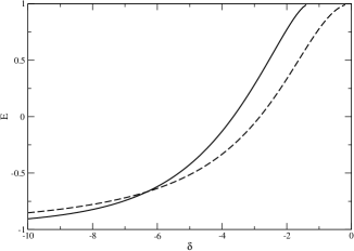
Figure 1: Solution curves of (33) (solid line) and (36) (dashed line) as a function of $\delta$, respectively.

By inserting (31) in (30), we obtain the spectral equation (bound states energy equation)

$$\frac{\delta}{v_{F}}\sqrt{\left(E+v_{F}^{2}m_{l}\right)\left(E+v_{F}^{2}m_{r}\right)}+\sqrt{\left(v_{F}^{4}m_{l}^{2}+1\right)\left(v_{F}^{2}m_{l}-E\right)\left(E+v_{F}^{2}m_{r}\right)}\\ +\sqrt{\left(v_{F}^{4}m_{r}^{2}+1\right)\left(E+v_{F}^{2}m_{l}\right)\left(v_{F}^{2}m_{r}-E\right)}=0$$ (33)

The energy of bound states lies between $-min(m_{l}v_{F}^{2},m_{r}v_{F}^{2})$ and $min(m_{l}v_{F}^{2},m_{r}v_{F}^{2})$. Note that equation (33) is invariant under the change of $m_{l}$ by $m_{r}$.

For $m_{l}=1,\,m_{r}=2$ and $v_{F}=1$, the solution curve of (33) as a function of $\delta$ is represented in the Figure 1. The solution curves intersect at a point, which means that they have the same energy for a given value of $\delta$. The value of the energy is insensitive to ratio of the masses.

As stated in [26], the boundary of the lower continuum is never reached for finite values of $\delta$ due to the presence of the scalar potential term, but the energy level crosses zero because of the vector potential term (see Figure 1).

For $m_{l}\approx m_{r}\equiv m$, (33) becomes

$$2v_{F}\sqrt{\left(v_{F}^{4}m^{2}+1\right)\left(v_{F}^{4}m^{2}-E^{2}\right)}+\delta\sqrt{\left(E+v_{F}^{2}m\right)^{2}}=0,$$ (34)

which gives the value of the energy for bound state

$$E=mv_{F}^{2}\;\frac{4v_{F}^{2}+4m^{2}v_{F}^{6}-\delta^{2}}{4v_{F}^{2}+4m^{2}v_{F}^{6}+\delta^{2}}$$ (35)

Defining $\tilde{\delta}=\frac{\delta}{v_{F}\sqrt{1+m^{2}v_{F}^{4}}}$, the above expression can be rewritten as

$$E=mv_{F}^{2}\frac{4-\tilde{\delta}^{2}}{4+\tilde{\delta}^{2}}$$ (36)

The energy (36) coincides with the one found in [26] and [27] for the self-adjoint extension called equally mixed potential.

At high energies, we have

$$\left|t_{l}\right|^{2}\sim\frac{4v_{F}^{2}\sqrt{\left(v_{F}^{4}m_{l}^{2}+1\right)\left(v_{F}^{4}m_{r}^{2}+1\right)}}{v_{F}^{2}\left(\sqrt{v_{F}^{4}m_{l}^{2}+1}+\sqrt{v_{F}^{4}m_{r}^{2}+1}\right)^{2}+\delta^{2}}$$ (37)

so that the transmission does not occur as the potential becomes sufficiently strong. Therefore, the interaction equally mixed PIP at the origin plus mass jump at the same point does confine particles. The same conclusion is reported in [26].

3.2 One - dimensional spatial Dirac Hamiltonian with a inverted mixed PIP at the origin plus mass jump at the same point

The matching conditions for this self -adjoint extension are

$$\begin{pmatrix}\phi_{a}(0^{+})\\ \phi_{b}(0^{+})\end{pmatrix}=\begin{pmatrix}\frac{(1+m_{r}^{2}v_{F}^{4})^{\frac{1}{4}}}{(1+m_{l}^{2}v_{F}^{4})^{\frac{1}{4}}}&\;-i\,\lambda\,v_{F}\,((1+m_{l}^{2}v_{F}^{4})(1+m_{r}^{2}v_{F}^{4}))^{\frac{1}{4}}\\ 0&\;\frac{(1+m_{l}^{2}v_{F}^{4})^{\frac{1}{4}}}{(1+m_{r}^{2}v_{F}^{4})^{\frac{1}{4}}}\end{pmatrix}\begin{pmatrix}\phi_{a}(0^{-})\\ \phi_{b}(0^{-})\end{pmatrix}$$ (38)

where $\lambda$ is the strength of PIP, $\lambda>0$. The spectral equation is

$$\sqrt{\left(v_{F}^{4}m_{l}^{2}+1\right)\left(v_{F}^{2}m_{l}-E\right)\left(E+v_{F}^{2}m_{r}\right)}+\sqrt{\left(v_{F}^{4}m_{r}^{2}+1\right)\left(E+v_{F}^{2}m_{l}\right)\left(v_{F}^{2}m_{r}-E\right)}\\ -v_{F}\,\lambda\sqrt{v_{F}^{2}m_{r}-E}\sqrt{v_{F}^{2}m_{l}-E}\sqrt{\left(v_{F}^{4}m_{l}^{2}+1\right)\left(v_{F}^{4}m_{r}^{2}+1\right)}=0,$$ (39)

where $-min\left(m_{l}v_{F}^{2},m_{r}v_{F}^{2}\right)<E<min\left(m_{l}v_{F}^{2},m_{r}v_{F}^{2}\right)$. This equation is invariant under the change of $m_{l}$ by $m_{r}$.

For $m_{l}\approx m_{r}\equiv m$, (39) becomes

$$2\sqrt{\left(v_{F}^{4}m^{2}-E^{2}\right)}-v_{F}\,\lambda\sqrt{\left(v_{F}^{4}m^{2}+1\right)}\left(v_{F}^{2}m-E\right)=0,$$ (40)

which gives the value of the energy for bound state

$$E=-mv_{F}^{2}\;\frac{4-\tilde{\lambda}^{2}}{4+\tilde{\lambda}^{2}},$$ (41)

with $\tilde{\lambda}\equiv v_{F}\,\sqrt{1+m^{2}v_{F}^{4}}\,\lambda$. The energy (41) coincides with the one found in [26] and [27] for the self-adjoint extension called inverted mixed potential.

Figure 2: Solution curves of (39) (solid line) and (41) (dashed line) as a function of $\lambda$, respectively.

For $m_{l}=1,\,m_{r}=2$ and $v_{F}=1$, the solution curve of (39) as a function of $\lambda$ is represented in the Figure 2. The solution curves intersect at a point, which means that they have the same energy for $\lambda=0.6324$. For weak coupling, the bound-states energy reaches the lower negative continuum, as distinct from that shown in [26].

At high energies, the transmission coefficient becomes

$$\left|t_{l}\right|^{2}\sim\frac{4\sqrt{v_{F}^{4}m_{l}^{2}+1}\sqrt{v_{F}^{4}m_{r}^{2}+1}}{\left(\sqrt{v_{F}^{4}m_{l}^{2}+1}+\sqrt{v_{F}^{4}m_{r}^{2}+1}\right)^{2}+v_{F}^{2}\left(v_{F}^{4}m_{l}^{2}+1\right)\left(v_{F}^{4}m_{r}^{2}+1\right)\lambda^{2}}$$ (42)

so that the transmission does not occur as the potential becomes sufficiently strong. As in the previous subsection, the interaction inverted mixed PIP at the origin plus mass jump at the same point does confine particles. This same conclusion is reported in [26] for this self-adjoint extension.

3.3 One - dimensional spatial Dirac Hamiltonian with a pure scalar PIP at the origin plus mass jump at the same point

The boundary conditions corresponding to one - dimensional spatial Dirac Hamiltonian with a pure scalar PIP at the origin plus a mass jump at the same point are

$$\begin{pmatrix}\phi_{a}(0^{+})\\ \phi_{b}(0^{+})\end{pmatrix}=\begin{pmatrix}\frac{(1+m_{r}^{2}v_{F}^{4})^{\frac{1}{4}}}{(1+m_{l}^{2}v_{F}^{4})^{\frac{1}{4}}}\cosh{\left(\frac{a}{v_{F}}\right)}&i\sinh{\left(\frac{a}{v_{F}}\right)}\\ -i\sinh{\left(\frac{a}{v_{F}}\right)}&\frac{(1+m_{l}^{2}v_{F}^{4})^{\frac{1}{4}}}{(1+m_{r}^{2}v_{F}^{4})^{\frac{1}{4}}}\cosh{\left(\frac{a}{v_{F}}\right)}\end{pmatrix}\begin{pmatrix}\phi_{a}(0^{-})\\ \phi_{b}(0^{-})\end{pmatrix}$$ (43)

where $a$ is the strength of PIP, $a<0$. The spectral equation is

$$\sqrt[4]{v_{F}^{4}m_{l}^{2}+1}\sqrt[4]{v_{F}^{4}m_{r}^{2}+1}\Big{(}\sqrt{v_{F}^{2}m_{l}-E}\sqrt{v_{F}^{2}m_{r}-E}\\ +\sqrt{E+v_{F}^{2}m_{l}}\sqrt{E+v_{F}^{2}m_{r}}\Big{)}\sinh\left(\frac{a}{v_{F}}\right)+\Big{(}\sqrt{v_{F}^{4}m_{l}^{2}+1}\sqrt{(v_{F}^{2}m_{l}-E)(E+v_{F}^{2}m_{r})}\\ +\sqrt{v_{F}^{4}m_{r}^{2}+1}\sqrt{(E+v_{F}^{2}m_{l})(v_{F}^{2}m_{r}-E)}\Big{)}\cosh\left(\frac{a}{v_{F}}\right)=0,$$ (44)

where $-min\left(m_{l}v_{F}^{2},m_{r}v_{F}^{2}\right)<E<min\left(m_{l}v_{F}^{2},m_{r}v_{F}^{2}\right)$. This equation is invariant under the change of $m_{l}$ by $m_{r}$.

Pairs of allowed energy values appear, which is a common feature of the other scalar-type potentials [28]. As seen in Figure 3, the same strength $a$ of the scalar potential can bind particles and antiparticles alike. As stated in [26], the energy level never reaches zero. The positive and negative energy states remain well separated even if the potential becomes strong.

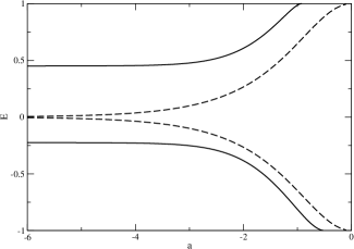
Figure 3: Solution curves of (44) (solid line) and (46) (dashed line) as a function of $a$, respectively, for $m_{l}=1$, $m_{r}=2$ and $v_{F}=1$.

For $m_{l}\approx m_{r}\equiv m$, (44) becomes

$$\sqrt{v_{F}^{4}m^{2}-E^{2}}\cosh\left(\frac{a}{v_{F}}\right)+v_{F}^{2}m\sinh\left(\frac{a}{v_{F}}\right)=0,$$ (45)

which gives the value of the energies for bound states

$$E=\pm\,mv_{F}^{2}\,\text{sech}\left(\frac{a}{v_{F}}\right).$$ (46)

The energy (46) coincides with the one found in [26] for the self-adjoint extension called pure scalar potential. For this potential, at hight energy, the transmission coefficient becomes

$$\left|t_{l}\right|^{2}\sim 4\,\frac{\sqrt{(1+v_{F}^{4}m_{l}^{2})(1+v_{F}^{4}m_{r}^{2})}\,}{\left(\sqrt{1+v_{F}^{4}m_{l}^{2}}+\sqrt{1+v_{F}^{4}m_{r}^{2}}\right)^{2}}\,\text{sech}^{2}\left(\frac{a}{v_{F}}\right)$$ (47)

Thus, the pure scalar potential leads to particle confinement when $\left|a\right|\rightarrow\infty$ .

3.4 One - dimensional spatial Dirac Hamiltonian with a pure vector PIP at the origin plus mass jump at the same point

The boundary conditions corresponding to one - dimensional spatial Dirac Hamiltonian with a pure vector PIP at the origin plus a mass jump at the same point are

$$\begin{pmatrix}\phi_{a}(0^{+})\\ \phi_{b}(0^{+})\end{pmatrix}=\begin{pmatrix}\frac{m_{r}}{m_{l}}\cos{\left(\frac{a}{v_{F}}\right)}&-i\sin{\left(\frac{a}{v_{F}}\right)}\\ -i\sin{\left(\frac{a}{v_{F}}\right)}&\frac{m_{l}}{m_{r}}\cos{\left(\frac{a}{v_{F}}\right)}\end{pmatrix}\begin{pmatrix}\phi_{a}(0^{-})\\ \phi_{b}(0^{-})\end{pmatrix}$$ (48)

with $a>0$, contrary to the assertion in [26], where the sign of the strength $a$ is immaterial as far as the existence of bound states.

The spectral equation is

$$\left(m_{l}^{2}\sqrt{v_{F}^{2}m_{r}+E}\sqrt{v_{F}^{2}m_{l}-E}+m_{r}^{2}\sqrt{v_{F}^{2}m_{l}+E}\sqrt{v_{F}^{2}m_{r}-E}\right)\cos\left(\frac{a}{v_{F}}\right)\\ +m_{r}m_{l}\Big{(}\sqrt{v_{F}^{2}m_{r}+E}\sqrt{v_{F}^{2}m_{l}+E}-\sqrt{v_{F}^{2}m_{l}-E}\sqrt{v_{F}^{2}m_{r}-E}\Big{)}\sin\left(\frac{a}{v_{F}}\right)=0,$$ (49)

where $-min\left(m_{l}v_{F}^{2},m_{r}v_{F}^{2}\right)<E<min\left(m_{l}v_{F}^{2},m_{r}v_{F}^{2}\right)$. Unlike the previous cases, (49) is not invariant under the change of $m_{l}$ by $m_{r}$. For $m_{l}=1,\,m_{r}=2$ and $v_{F}=1$, the solution curve of (49) as a function of $a$ is represented in the Figure 4.

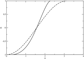
Figure 4: Solution curves of (49) (solid line) and (51) (dashed line) as a function of $a$, respectively, for $m_{l}=1$, $m_{r}=2$ and $v_{F}=1$.

For $m_{l}\approx m_{r}\equiv m$, (49) becomes

$$\sqrt{v_{F}^{4}m^{2}-E^{2}}\cos\left(\frac{a}{v_{F}}\right)+E\sin\left(\frac{a}{v_{F}}\right)=0,$$ (50)

which gives the value of the energies for bound states

$$E=\pm\,mv_{F}^{2}\,\cos\left(\frac{a}{v_{F}}\right).$$ (51)

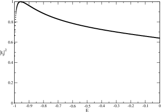
Figure 5: Transmission resonances for $a=\pi$, $m_{l}=1$, $m_{r}=2$ and $v_{F}=1$.

The transmission coefficient is bounded from below,

$$\left|t_{l}\right|^{2}\geq\frac{8m_{l}^{2}m_{r}^{2}\sqrt{E-v_{F}^{2}m_{l}}\sqrt{E+v_{F}^{2}m_{l}}\sqrt{E-v_{F}^{2}m_{r}}\sqrt{E+v_{F}^{2}m_{r}}}{4m_{l}^{2}m_{r}^{2}\sqrt{E-v_{F}^{2}m_{l}}\sqrt{E+v_{F}^{2}m_{l}}\sqrt{E-v_{F}^{2}m_{r}}\sqrt{E+v_{F}^{2}m_{r}}+E^{2}\left(m_{l}^{2}+m_{r}^{2}\right)^{2}}$$ (52)

so that the transmission always occurs. There are transmission resonances or virtual bound states [29] for values $\frac{a}{v_{F}}=n\pi$, $n\in\mathbb{Z}$ (see Figures 5 and 6).

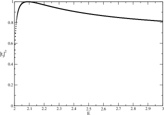
Figure 6: Transmission resonances for $a=\pi$, $m_{l}=1$, $m_{r}=2$ and $v_{F}=1$.

4 Concluding remarks

Using the Von Neumann’s theory of self-adjoint extensions and eliminating spurious phases of the transmission amplitude, we found the general matching conditions (28) that describe each one of the different domains of the various self-adjoint extensions of (2). Using the scattering theory, we obtained the spectrum of each one of the extensions, where each corresponds to a different Hamiltonian operator with interaction.

Finally, we found that of the four different self-adjoint extensions of (2), the first three are confining self-adjoint extensions, while the latter is not. For three of the self-adjoint extensions, there is a value of the strength of the interaction point which the energy of the particle is the same for the mass jump case and without it.

5 Acknowledgments

This work was supported by IVIC under Project No. 1089.

6 References

References

- [1] K. S. Novoselov, A. K. Geim, S. V. Morozov, D. Jiang, Y. Zhang, S. V. Dubonos, V. I. Grigorieva and A. A. Firsov 2004 Science 306 666
- [2] K. S. Novoselov, D. Jiang, T. Booth, V. V. Khotkevich, S. V. Morozov and A. K. Geim 2005 Proc. Natl. Acad. Sci. 102 10451
- [3] S. -L. Zhu, B. Wang, T. Booth, L. -M. Duan 2007 Phys. Rev. Lett. 98 260402
- [4] J. Ruostekoski, J. Javanainen, and G. V. Dunne, L. -M. Duan 2008 Phys. Rev. A 77 013603
- [5] K. K. Gomes, W. Mar, W. Ko, F. Guinea, and H. C. Manoharan 2012 Nature (London) 483 306
- [6] D. -W. Zhang, L. -B. Shao, Z. -Y. Xue, H. Yan, Z. D. Wang, and S. -L. Zhu 2012 Phys. Rev. A 86 063616
- [7] C. Yannouleas, I. Romanovsky, and U. Landman 2014 Phys. Rev. B 89 035432
- [8] V. I. Tamarchenko and S. A. Ktitorov 1978 Sov. Phys. Solid State 19 1211
- [9] Natalie E. Firsova, Sergey A. Ktitorov, Philip A. Pogorelov 2009 Phys. Lett. A 373 525
- [10] Natalie E. Firsova, Sergey A. Ktitorov 2010 Phys. Lett. A 374 1270
- [11] S. A. Ktitorov and Natalie E. Firsova 2011 Phys. Solid State 53 411
- [12] V. Jakubský and D. Krejčiřík 2014 Ann. Phys. 349 268
- [13] M. Asorey, A. Ibort, G. Marmo 2005 Int. J. Mod. Phys. A 20 1001
- [14] M. Asorey, A. Ibort, G. Marmo 2012 Int. J. Geom. Methods Mod. Phys. 9 1260017
- [15] H. B. G. Casimir 1948 Proc. K. Ned. Akad. Wet. 51 793
- [16] V. John, G. Jungman, and S. Vaidya 1995 Nucl. Phys. B 455 505
- [17] D. J. Thouless, M. Kohmoto, M. P. Nightingale, and M. den Nijs 1982 Phys. Rev. Lett. 49 405
- [18] M. Reed and B. Simon, Methods of Modern Mathematical Physics II: Fourier Analysis, Self - Adjointness, Academic Press Inc., San Diego, California, 1975.
- [19] M. A. Naimark, Linear Differential Operators. Vol II, Frederick Ungar Publishing Company, New York, 1968.
- [20] Y. Nogami and C. K. Ross 1996 Am. J. Phys. 64, 923
- [21] F. A. B. Coutinho, Y. Nogami and J. Fernando Perez 1988 J. Phys. A: Math. Gen. 32 L133
- [22] L. A. González-Díaz and S. Díaz-Solórzano 2013 J. Math. Phys. 54 042106
- [23] R. G. Newton, Scattering Theory of Waves and Particles, McGraw - Hill, Inc., New York, 1966.
- [24] J. R. Taylor, Scattering Theory: The Quantum Theory on Nonrelativistic Collisions, John Wiley & Sons, Inc., New York, 1972.
- [25] N. Dombey, P. Kennedy and A. Calogeracos 2000 Phys Rev Lett. 85 1787
- [26] F. Domínguez - Adame and E. Maciá 1989 J. Phys. A 22 L419
- [27] S. Albeverio, F. Gesztesy, R. Høegh-Krohn and H. Holden, Solvable Models in Quantum Mechanics, Second Edition, AMS, 2005.
- [28] F. A. B. Coutinho, Y. Nogami and F. M. Toyama 1988 Am. J. Phys. 56 904
- [29] A. Galindo and P. Pascual, Mecánica Cuántica, Editorial Alhambra, Madrid. 1978.