Modeling TB-HIV syndemic and treatment

Abstract

Tuberculosis (TB) and human immunodeficiency virus (HIV) can be considered a deadly human syndemic. In this article, we formulate a model for TB and HIV transmission dynamics. The model considers both TB and acquired immune deficiency syndrome (AIDS) treatment for individuals with only one of the infectious diseases or both. The basic reproduction number and equilibrium points are determined and stability is analyzed. Through simulations, we show that TB treatment for individuals with only TB infection reduces the number of individuals that become co-infected with TB and HIV/AIDS, and reduces the diseases (TB and AIDS) induced deaths. Analogously, the treatment of individuals with only AIDS also reduces the number of co-infected individuals. Further, TB-treatment for co-infected individuals in the active and latent stage of TB disease, implies a decrease of the number of individuals that passes from HIV-positive to AIDS.

Keywords:

Tuberculosis, Human immunodeficiency virus, Syndemic, Treatment, Equilibrium, Stability.

Mathematics Subject Classification 2010:

34D30; 92D30; 93A30.

1 Introduction

Tuberculosis (TB) and human immunodeficiency virus/acquired immune deficiency syndrome (HIV/AIDS) are the leading causes of death from an infectious disease worldwide [16]. Individuals infected with HIV are more likely to develop TB disease because of their immunodeficiency, and HIV infection is the most powerful risk factor for progression from TB infection to disease [7]. This interaction justifies the fact that HIV and TB can be considered a deadly human syndemic, where syndemic refers to the convergence of two or more diseases that act synergistically to magnify the burden of disease [10].

Following UNAIDS global report on AIDS epidemic 2013 [14], globally, an estimated 35.3 million people were living with HIV in 2012. An increase from previous years, as more people are receiving the life-saving antiretroviral therapy (ART). There were approximately 2.3 million new HIV infections globally, showing a 33% decline in the number of new infections with respect to 2001. At the same time, the number of AIDS deaths is also declining with around 1.6 million AIDS deaths in 2012, down from about 2.3 million in 2005. In 2012, 1.1 million of 8.6 million people who developed TB worldwide were HIV-positive. The number of people dying from HIV-associated TB has been falling since 2003. However, there were still 320 000 deaths from HIV-associated TB in 2012 and further efforts are needed to reduce this burden [16]. ART is a critical intervention for reducing the risk of TB morbidity and mortality among people living with HIV and, when combined with isoniazid preventive therapy, it can have a significant impact on TB prevention [16].

Collaborative TB/HIV activities (including HIV testing, ART therapy and TB preventive measures) are crucial for the reduction of TB-HIV coinfected individuals. The World Health Organization (WHO) estimates that these collaborative activities prevented 1.3 million people from dying, from 2005 to 2012. However, significant challenges remain: the reduction of tuberculosis related deaths among people living with HIV has slowed in recent years; the ART therapy is not being delivered to TB-HIV coinfected patients in the majority of the countries with the largest number of TB/HIV patients; the pace of treatment scale-up for TB/HIV patients has slowed; less than half of notified TB patients were tested for HIV in 2012; and only a small fraction of TB/HIV infected individuals received TB preventive therapy [14].

The study of the joint dynamics of TB and HIV present formidable mathematical challenges due to the fact that the models of transmission are quite distinct [12]. Few mathematical models have been proposed for TB-HIV coinfection (see, for example, [1, 9, 11, 12, 13]). Kirschner [9] developed a cellular model for HIV-1 and TB coinfection inside a host. Roeger et al. [12] proposed a population model for TB-HIV/AIDS coinfection transmission dynamics, assuming that TB-infected individuals in the active stage of the disease are too ill to remain sexually active and therefore they are unable to transmit HIV. In this work we assume that active TB-infected individuals are susceptible to HIV-infection. Naresh and Tripathi [11] proposed a model for TB-HIV coinfection in a variable size population with only TB treatment. Here we consider TB and HIV treatment in different stages of the disease. Bhunu et al. [1] studied a TB-HIV coinfection model with both TB and HIV treatment. The authors did not take into account that an individual co-infected with TB and HIV can effectively recover from TB infection. We assume that TB can be cured, even in HIV-positive individuals [16]. Sharomi et al. [13] also considered these assumptions, subdividing the total population into 15 classes. It is our aim in this work to develop a model that balances two goals: simplicity and useful information.

The paper is organized as follows. Section 2 describes our model for TB-HIV syndemic with TB and HIV treatment. In Section 3 the positivity and boundedness of solutions of the model are proved and in Section 4 equilibrium points and respective stability are analyzed. Section 5 is devoted to numerical simulations and discussion of results.

2 TB-HIV/AIDS model

The model subdivides the human population into 10 mutually-exclusive compartments, namely susceptible individuals ($S$), TB-latently infected individuals, who have no symptoms of TB disease and are not infectious ($L_{T}$), TB-infected individuals, who have active TB disease and are infectious ($I_{T}$), TB-recovered individuals ($R_{T}$), HIV-infected individuals with no clinical symptoms of AIDS ($I_{H}$), HIV-infected individuals with AIDS clinical symptoms ($A$), TB-latent individuals co-infected with HIV (pre-AIDS) ($L_{TH}$), HIV-infected individuals (pre-AIDS) co-infected with active TB disease ($I_{TH}$), TB-recovered individuals with HIV-infection without AIDS symptoms ($R_{TH}$), HIV-infected individuals with AIDS symptoms co-infected with TB ($A_{T}$). The total population at time $t$, denoted by $N(t)$, is given by

$$N(t)=S(t)+L_{T}(t)+I_{T}(t)+R_{T}(t)+I_{H}(t)+A(t)+I_{TH}(t)+L_{TH}(t)+R_{TH}(t)+A_{T}(t)\,.$$

The susceptible population is increased by the recruitment of individuals (assumed susceptible) into the population, at a rate $\Lambda$. All individuals suffer from natural death, at a constant rate $\mu$. Susceptible individuals acquire TB infection from individuals with active TB at a rate $\lambda_{T}$, given by

$$\lambda_{T}=\frac{\beta_{1}}{N}\left(I_{T}+I_{TH}+A_{T}\right)\,,$$

where $\beta_{1}$ is the effective contact rate for TB infection. Similarly, susceptible individuals acquire HIV infection, following effective contact with people infected with HIV at a rate $\lambda_{H}$, given by

$$\lambda_{H}=\frac{\beta_{2}}{N}\left[I_{H}+I_{TH}+L_{TH}+R_{TH}+\eta\left(A+A_{T}\right)\right]\,,$$

where $\beta_{2}$ is the effective contact rate for HIV transmission and the modification parameter $\eta\geqslant 1$ accounts for the relative infectiousness of individuals with AIDS symptoms, in comparison to those infected with HIV with no AIDS symptoms. Individuals with AIDS symptoms are more infectious than HIV-infected individuals (pre-AIDS) because they have a higher viral load and there is a positive correlation between viral load and infectiousness [5].

Individuals leave the latent-TB class $L_{T}$ by becoming infectious, at a rate $k_{1}$, or recovered, with a treatment rate $\tau_{1}$. The treatment rate for active TB-infected individuals is $\tau_{2}$. We assume that TB-recovered individuals $R_{T}$ acquire partial immunity and the transmission rate for this class is given by $\beta^{\prime}_{1}\lambda_{T}$ with $\beta^{\prime}_{1}\leqslant 1$. Individuals with active TB disease suffer induced death at a rate $d_{T}$. We assume that individuals in the class $R_{T}$ are susceptible to HIV infection at a rate $\lambda_{H}$. On the other hand, TB-active infected individuals $I_{T}$ are susceptible to HIV infection, at a rate $\delta\lambda_{H}$, where the modification parameter $\delta\geqslant 1$ accounts for higher probability of individuals in class $I_{T}$ to become HIV-positive.

HIV-infected individuals (with no AIDS symptoms) progress to the AIDS class $A$, at a rate $\rho_{1}$. HIV-infected individuals with AIDS symptoms are treated for HIV at the rate $\alpha_{1}$ and suffer induced death at a rate $d_{A}$. Individuals in the class $I_{H}$ are susceptible to TB infection at a rate $\psi\lambda_{T}$, where $\psi\geqslant 1$ is a modification parameter traducing the fact that HIV infection is a driver of TB epidemic [10].

HIV-infected individuals (pre-AIDS) co-infected with TB-disease, in the active stage $I_{TH}$, are treated for TB at the rate $\tau_{3}$ and progress to the AIDS-TB co-infection class $A_{T}$ at a rate $\rho_{2}$. Individuals in the class $I_{TH}$ suffer TB induced death at a rate $d_{T}$. The anti-TB drugs can prevent or decrease the likelihood of TB infection progression to active TB disease in individuals in the class $L_{TH}$ [17]. The treatment rate for individuals in this class is given by $\tau_{4}$. However, individuals in the class $L_{TH}$ are more likely to progress to active TB disease than individuals infected only with latent TB. In our model, this progression rate is given by $k_{2}$. Similarly, HIV infection makes individuals more susceptible to TB reinfection when compared with non HIV-positive patients. The modification parameter associated to the TB reinfection rate, for individuals in the class $R_{TH}$, is given by $\beta^{\prime}_{2}$, where $\beta^{\prime}_{2}\geqslant 1$. Individuals in this class progress to class $A_{T}$, at a rate $\rho_{3}$.

HIV-infected individuals (with AIDS symptoms), co-infected with TB, are treated for HIV, at a rate $\alpha_{2}$. Individuals in the class $A_{T}$ suffer from AIDS-TB coinfection induced death rate, at a rate $d_{TA}$.

The aforementioned assumptions result in the following system of differential equations that describes the transmission dynamics of TB and HIV disease:

$$\begin{cases}\dot{S}(t)=\Lambda-\lambda_{T}S(t)-\lambda_{H}S(t)-\mu S(t),\\[5.69046pt] \dot{L}_{T}(t)=\lambda_{T}S(t)+\beta^{{}^{\prime}}_{1}\lambda_{T}R_{T}(t)-(k_{1}+\tau_{1}+\mu)L_{T}(t),\\[5.69046pt] \dot{I}_{T}(t)=k_{1}L_{T}(t)-(\tau_{2}+d_{T}+\mu+\delta\lambda_{H})I_{T}(t),\\[5.69046pt] \dot{R}_{T}(t)=\tau_{1}L_{T}(t)+\tau_{2}I_{T}(t)-(\beta^{{}^{\prime}}_{1}\lambda_{T}+\lambda_{H}+\mu)R_{T}(t),\\[5.69046pt] \dot{I}_{H}(t)=\lambda_{H}S(t)-(\rho_{1}+\psi\lambda_{T}+\mu)I_{H}(t)+\alpha_{1}A(t)+\lambda_{H}R_{T}(t),\\[5.69046pt] \dot{A}(t)=\rho_{1}I_{H}(t)-\alpha_{1}A(t)-(\mu+d_{A})A(t),\\[5.69046pt] \dot{L}_{TH}(t)=\beta^{{}^{\prime}}_{2}\lambda_{T}R_{TH}(t)-(k_{2}+\tau_{4}+\mu)L_{TH}(t),\\[5.69046pt] \dot{I}_{TH}(t)=\delta\lambda_{H}I_{T}(t)+\psi\lambda_{T}I_{H}(t)+\alpha_{2}A_{T}(t)+k_{2}L_{TH}(t)-(\tau_{3}+\rho_{2}+\mu+d_{T})I_{TH}(t),\\[5.69046pt] \dot{R}_{TH}(t)=\tau_{3}I_{TH}(t)+\tau_{4}L_{TH}(t)-(\beta^{{}^{\prime}}_{2}\lambda_{T}+\rho_{3}+\mu)R_{TH},\\[5.69046pt] \dot{A}_{T}(t)=\rho_{2}I_{TH}(t)+\rho_{3}R_{TH}-(\alpha_{2}+\mu+d_{TA})A_{T}(t)\,.\end{cases}$$ (1)

The model flow is described in Figure 1.

Figure 1: Model for TB-HIV/AIDS transmission with treatment.

The initial conditions of model (1) satisfy

$$\begin{split}&S(0)=S_{0}\geqslant 0\,,\quad\quad L_{T}(0)=L_{T0}\geqslant 0\,,\quad\quad I_{T}(0)=I_{T0}\geqslant 0\,,\quad\quad R_{T}(0)=R_{T0}\geqslant 0\,,\\ &I_{H}(0)=I_{H0}\geqslant 0\,,\quad\quad A(0)=A_{0}\geqslant 0\,,\quad\quad L_{TH}(0)=L_{TH0}\geqslant 0\,,\\ &I_{TH}(0)=I_{TH0}\geqslant 0\,,\quad\quad R_{TH}(0)=R_{TH0}\geqslant 0\,,\quad\quad A_{T}(0)=A_{T0}\geqslant 0\,.\end{split}$$ (2)

Note that if we consider the sub-model of (1) with no HIV/AIDS disease, that is, $I_{H}=A=L_{TH}=I_{TH}=R_{TH}=A_{T}=0$, then we obtain the TB model from [3]. On the other hand, if we consider the sub-model with no TB, that is, $L_{T}=I_{T}=R_{T}=L_{TH}=I_{TH}=R_{TH}=A_{T}=0$, then we obtain an HIV/AIDS model based on the models proposed in [1, 8].

3 Positivity and boundedness of solutions

Let $(S,L_{T},I_{T},R_{T},I_{H},A,L_{TH},I_{TH},R_{TH},A_{T})\in\mathbb{R}^{10}_{+}$ be any solution of (1) with initial conditions (2). Consider the biologically feasible region given by

$$\Omega=\left\{\left(S,L_{T},I_{T},R_{T},I_{H},A,L_{TH},I_{TH},R_{TH},A_{T}\right)\,\in\mathbb{R}^{10}_{+}\,:\,0\leqslant N(t)\leqslant\frac{\Lambda}{\mu}\right\}\,.$$ (3)

For the model system (1) to be epidemiologically meaningful, it is important to prove that all its state variables are nonnegative for all time $t>0$. Suppose, for example, that at some $\bar{t}>0$ the variable $L_{T}$ becomes zero, i.e., $L_{T}(\bar{t})=0$, while all other variables are positive. Then, from the $L_{T}$ equation we have $dL_{T}(\bar{t})/dt>0$. Thus, $L_{T}(t)\geqslant 0$ for all $t>0$. Analogously, we can prove that all variables remain nonnegative for all time $t>0$.

Adding all equations in model (1) gives

$$\frac{dN}{dt}(t)=\Lambda-\mu N(t)-d_{T}I_{T}(t)-d_{A}A(t)-d_{T}I_{TH}(t)-d_{TA}A_{T}(t)\,.$$

Since $N(t)\geqslant I_{T}(t)+A(t)+I_{TH}(t)+A_{T}(t)$, then

$$\Lambda-(\mu+d_{T}+d_{A}+d_{TA})N(t)\leqslant\frac{dN}{dt}(t)\leqslant\Lambda-\mu N(t)\,.$$

Therefore, we conclude that $N(t)$ is bounded for all $t>0$ and every solution of system (1) with initial condition in $\Omega$ remains in $\Omega$. This result is summarized below.

Lemma 3.1.

The region $\Omega$ is positively invariant for the model (1) with non-negative initial conditions in $\mathbb{R}^{10}_{+}$.

4 Stability analysis

The model (1) has four non-negative equilibria, namely

• The disease-free equilibrium (no disease)

  $$\Sigma_{0}=\left(S_{0},L_{T_{0}},I_{T_{0}},R_{T_{0}},I_{H_{0}},A_{0},L_{TH_{0}},I_{TH_{0}},R_{TH_{0}},A_{T_{0}}\right)=\left(\frac{\Lambda}{\mu},0,0,0,0,0,0,0,0,0\right)\,.$$ (4)

• The HIV-AIDS free equilibrium

  $$\Sigma_{T}=\left(S^{\diamond},L_{T}^{\diamond},I_{T}^{\diamond},R_{T}^{\diamond},I_{H}^{\diamond},A^{\diamond},L_{TH}^{\diamond},I_{TH}^{\diamond},R_{TH}^{\diamond},A_{T}^{\diamond}\right)$$

  with $I_{T}^{\diamond}>0$ and $I_{H}^{\diamond}=A^{\diamond}=L_{TH}^{\diamond}=I_{TH}^{\diamond}=R_{TH}^{\diamond}=A_{T}^{\diamond}=0$ for $R_{1}>1$, where $R_{1}$ is the basic reproduction number of the model (1) with $I_{H}=A=L_{TH}=I_{TH}=R_{TH}=A_{T}=0$ (only TB model) that is given by

  $$R_{1}=\frac{\Lambda}{N\mu}\left(\frac{\beta_{1}}{d_{T}+\mu+\tau_{2}}\right)\left(\frac{k_{1}}{k_{1}+\tau_{1}+\mu}\right)$$ (5)

  (see [3]).

• The TB-free equilibrium

  $$\Sigma_{H}=\left(S^{\star},L_{T}^{\star},I_{T}^{\star},R_{T}^{\star},I_{H}^{\star},A^{\star},L_{TH}^{\star},I_{TH}^{\star},R_{TH}^{\star},A_{T}^{\star}\right)$$

  with $L_{T}^{\star}=I_{T}^{\star}=R_{T}^{\star}=L_{TH}^{\star}=I_{TH}^{\star}=R_{TH}^{\star}=A_{T}^{\star}=0$ and

  $$S^{\star}=\frac{\Lambda}{\mu R_{2}}\,,\quad I_{H}^{\star}=(R_{2}-1)\frac{\mu N_{H}(\alpha_{1}+d_{A}+\mu)}{\beta_{2}(\alpha_{1}+d_{A}+\mu+\eta\rho_{1})}\,,\,\,\quad A^{\star}=(R_{2}-1)\frac{\rho_{1}\mu N_{H}}{\beta_{2}(\alpha_{1}+d_{A}+\mu+\eta\rho_{1})},$$

  for $R_{2}>1$, where $R_{2}$ is the basic reproduction number of model (1) with $L_{T}=I_{T}=R_{T}=L_{TH}=I_{TH}=R_{TH}=A_{T}=0$ (only HIV-AIDS model), that is,

  $$R_{2}=\frac{\Lambda}{N\mu}\beta_{2}\left(\frac{\mu+\alpha_{1}+d_{A}+\eta\,\rho_{1}}{\mu\,\alpha_{1}+(\mu+\rho_{1})(\mu+d_{A})}\right)\,.$$ (6)

• The syndemic equilibrium

  $$\Sigma^{*}=(S^{*},L_{T}^{*},I_{T}^{*},R_{T}^{*},I_{H}^{*},A^{*},L^{*}_{TH},I_{TH}^{*},R_{TH}^{*},A_{T}^{*})$$

  with $I_{T}^{*}>0$, $I_{H}^{*}>0$, $A^{*}>0$, $L_{TH}^{*}>0$, $I_{TH}^{*}>0$, $R_{TH}^{*}>0$ and $A_{T}^{*}>0$, for $R_{0}>1$, where $R_{0}$ is the basic reproduction number of the model (1), that is,

  $$R_{0}=\max\{R_{1},R_{2}\}\,.$$

The details of the computation of the basic reproduction number $R_{0}$ are given in Appendix A.

The following theorem states the stability of the equilibrium points.

Theorem 4.1.

The disease free equilibrium $\Sigma_{0}$ is locally asymptotically stable if $R_{0}<1$, and unstable if either $R_{i}>1$ with $i=1,2$. The HIV-AIDS free equilibrium $\Sigma_{T}$ is locally asymptotically stable if $R_{1}>1$, and the TB-free equilibrium $\Sigma_{H}$ is locally asymptotically stable for $R_{2}$ near 1.

Details of the proof of Theorem 4.1 are given in Appendix B.

Explicit expressions for the coinfection endemic equilibrium $\Sigma^{*}$ are very difficult to compute analytically. In Section 5, we consider an example, with $R_{0}>1$, for which there exists a syndemic equilibrium, and analyze, numerically, the local asymptotical stability of the syndemic equilibrium $\Sigma^{*}$.

5 Numerical analysis and discussion

For numerical simulations, we consider the following initial conditions for system (1):

$$\left(S(0),L_{T}(0),I_{T}(0),R_{T}(0),I_{H}(0),A(0),L_{TH}(0),I_{TH}(0),R_{TH}(0),A_{T}(0)\right)\\ =\left(\frac{60N}{100},\frac{14N}{100},\frac{3N}{100},0,\frac{4N}{100},\frac{N}{100},\frac{12N}{100},\frac{5N}{100},0,\frac{N}{100}\right)$$ (7)

with $N=50000$. The parameters of model (1) take the values of Table 1.

Symbol	Value	References	Symbol	Value	References
$\Lambda$	$714$		$\tau_{4}$	$1\,yr^{-1}$
$\mu$	$1/70\,yr^{-1}$		$\rho_{1}$	$0.1\,yr^{-1}$	[18, 19]
$\beta_{1}$	variable		$\rho_{2}$	$0.25\,yr^{-1}$
$\beta_{2}$	variable		$\rho_{3}$	$0.125\,yr^{-1}$
$\beta^{\prime}_{1}$	$0.9$		$\alpha_{1}$	$0.33\,yr^{-1}$	[1]
$\beta^{\prime}_{2}$	$1.1$		$\alpha_{2}$	$0.33\,yr^{-1}$
$k_{1}$	$1$	[3]	$\psi$	$1.07$
$k_{2}$	$1.3\,k_{1}$	[17]	$d_{T}$	$1/8\,yr^{-1}$
$\tau_{1}$	$1\,yr^{-1}$	[3]	$d_{A}$	$0.3\,yr^{-1}$
$\tau_{2}$	$2\,yr^{-1}$	[3]	$d_{TA}$	$0.33\,yr^{-1}$
$\tau_{3}$	$2\,yr^{-1}$		$\eta$	$1.02$
$\delta$	$1.03$

Table 1: Parameters of the TB-HIV/AIDS model (1).

5.1 Equilibrium points and stability analysis

In Table 2 we show the effect of the transmission coefficient $\beta_{1}$ on the state $I_{T}^{\diamond}$ of the HIV-free equilibrium $\Sigma_{T}$ and on the basic reproduction number $R_{1}$. Table 3 shows the effect of the transmission coefficient $\beta_{2}$ on the states $I_{H}^{\star}$ and $A^{\star}$ of the TB-free equilibrium $\Sigma_{H}$ and on the basic reproduction number $R_{2}$. We conclude that the equilibrium states $I_{T}^{\diamond}$ and $(I_{H}^{\star},A^{\star})$ increase with the transmission coefficients $\beta_{1}$ and $\beta_{2}$, respectively.

$\beta_{1}$	4.3	6	10	15	50
$R_{1}$	0.99788	1.39239	2.32065	3.48097	11.60326
$I_{T}^{\diamond}$	0.00397	903.93492	2206.57268	2870.72755	3804.50589

Table 2: Effect of $\beta_{1}$ on $I_{T}^{\diamond}$ and $R_{1}$.

$\beta_{2}$	0.051	0.055	0.07	0.09	0.99
$R_{2}$	0.93669	1.01016	1.28566	1.65299	1.81829
$I_{H}^{\star}$	0.01708	135.73817	2516.54721	4472.84980	4930.48696
$A^{\star}$	0.00266	21.07182	390.59491	694.23361	765.26396

Table 3: Effect of $\beta_{2}$ on $I_{H}^{\star}$, $A^{\star}$ and $R_{2}$.

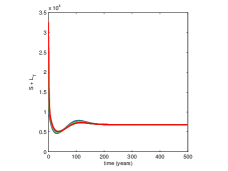
In Figure 2 we considered different initial conditions in a neighborhood of the initial conditions given by (7) and $R_{0}<1$ ($R_{1}<1$ and $R_{2}<1$) to illustrate the stability of the disease-free equilibrium $\Sigma_{0}$ given by (4). In these numerical simulations we considered $\beta_{1}=2.7$ and $\beta_{2}=0.03$, corresponding to $R_{1}=0.62632$ and $R_{2}=0.55077$, while the rest of the parameters take the values in Table 1.

$\begin{array}[]{cc}\includegraphics[scale={0.6}]{S_DFE_stability_V4.eps}&\includegraphics[scale={0.6}]{NmenosS_DFE_stab_V4.eps}\\ \end{array}$

Figure 2: Stability of the disease-free equilibrium (4).

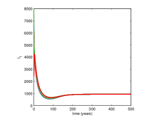
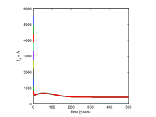
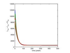
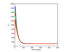
Figure 3 shows that, for $R_{0}>1$, the syndemic equilibrium $\Sigma^{*}$ exists. We considered different initial conditions for the state variables of system (1) in a neighborhood of (7), $\beta_{1}=6$ and $\beta_{2}=0.1$, corresponding to $R_{1}=1.39239$ and $R_{2}=1.83593$, and the rest of the parameters take the values in Table 1. We observe that the state variables converge to $\Sigma^{*}$ when $t\rightarrow\infty$. In this case, $\Sigma^{*}$ is given by

$$\begin{split}\Sigma^{*}&=\left(S^{*},L_{T}^{*},I_{T}^{*},R_{T}^{*},I_{H}^{*},A^{*},L^{*}_{TH},I_{TH}^{*},R_{TH}^{*},A_{T}^{*}\right)\\ &=(4766.84,2019.66,943.06,28621.89,362.66,56.29,31.39,55.15,495.68,112.33)\,.\end{split}$$

Figure 3: Stability of the syndemic equilibrium $\Sigma^{*}$.

5.2 Treatment impact on TB-HIV/AIDS coinfection

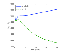
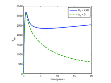
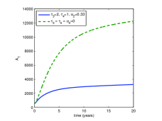
Consider $\beta_{1}=13$ and $\beta_{2}=0.06$, while the rest of the parameters take the values of Table 1. Figure 4 shows the impact of treating the individuals with active and latent TB on the number of individuals co-infected with TB-HIV/AIDS. The treatment of individuals with only-TB, $I_{T}$ and $L_{T}$, has a positive impact on the reduction of the number of individuals co-infected with TB-HIV/AIDS. Moreover, the number of individuals that suffered from disease (TB and AIDS) induced death is higher when individuals with TB-single infection are not treated. In this case the total population at the end of 20 years is around 10509 and, in the case where individuals with only TB are treated, the total population at the end of 20 years is around 29758 individuals. In Figure 5, we assume that there are no disease induced deaths, that is, $d_{T}=d_{A}=d_{TA}=0$. The impact of treating individuals with only TB on the reduction of the number of individuals co-infected is more evident.

Figure 4: Impact of TB treatment on single-infected individuals with disease induced death.

Figure 5: Impact of TB treatment on single-infected individuals with no disease induced death.

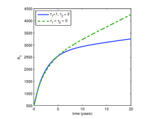
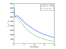
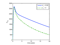
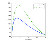
Figure 6 illustrates the case where we compare the number of individuals co-infected with TB-HIV/AIDS when individuals with only AIDS symptoms $A_{T}$ are or not treated. We observe that treating this class of individuals is important for the reduction of the number of individuals that become co-infected, with special attention to the individuals that have AIDS symptoms and TB infection. In figure 7, we considered that there is no disease induced deaths ($d_{T}=d_{A}=d_{TA}=0$).

Figure 6: Impact of AIDS treatment on single-infected individuals with disease induced death.

Figure 7: Impact of AIDS treatment on single-infected individuals with no disease induced death.

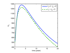
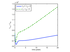
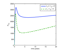
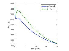
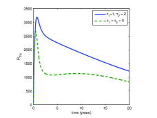
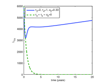
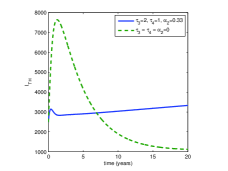
It is crucial that TB-infected individuals (in the latent and active stage), which are also HIV-positive, take anti-TB drugs, since they can recover from TB. We analyze the impact of treating TB-HIV/AIDS co-infected individuals $L_{TH}$, $I_{TH}$ and $A_{T}$ on the reduction of the number of individuals coinfection. If anti-TB drugs are supplied, then latent and active-TB individuals with HIV can recover and pass to the class $R_{TH}$ (the number of individuals in the class $R_{TH}$ tends to zero when TB is not treated). In Figure 8, we observe that after 7 years the number of individuals infected with active-TB and HIV, in the case without treatment, becomes lower than in the case with treatment. This is due to the fact that coinfection precipitates AIDS symptoms.

Figure 8: Impact of TB and AIDS treatment on co-infected individuals with no disease induced death.

Appendix A Appendix: Computation of $R_{0}$

The basic reproduction number represents the expected average number of new infections produced by a single infectious individual when in contact with a completely susceptible population [15]. Following [15], the basic reproduction number $R_{0}$ is obtained as the spectral radius of the matrix $F\cdot V^{-1}$ at the disease-free equilibrium $\Sigma_{0}$, given by (4), with $F=\left[\begin{array}[]{cc}F_{1}\quad F_{2}\end{array}\right]$ and

$$F_{1}=\left[\begin{array}[]{ccccc}0&0&0&0&0\\ \vskip 6.0pt plus 2.0pt minus 2.0pt\cr\lambda_{T}&0&{\frac{\beta_{1}S}{N}}+{\frac{\beta^{{}^{\prime}}_{1}\beta_{1}R_{T}}{N}}&\beta^{{}^{\prime}}_{1}\lambda_{T}&0\\ \vskip 6.0pt plus 2.0pt minus 2.0pt\cr 0&0&0&0&0\\ \vskip 6.0pt plus 2.0pt minus 2.0pt\cr 0&0&0&0&0\\ \vskip 6.0pt plus 2.0pt minus 2.0pt\cr\lambda_{H}&0&0&\lambda_{H}&{\frac{\beta_{2}S}{N}}+{\frac{\beta_{2}R_{T}}{N}}\\ \vskip 6.0pt plus 2.0pt minus 2.0pt\cr 0&0&0&0&0\\ \vskip 6.0pt plus 2.0pt minus 2.0pt\cr 0&0&{\frac{\beta^{{}^{\prime}}_{2}\beta_{1}R_{TH}}{N}}&0&0\\ \vskip 6.0pt plus 2.0pt minus 2.0pt\cr 0&0&\delta\lambda_{H}+{\frac{\psi\beta_{1}I_{H}}{N}}&0&{\frac{\delta\beta_{2}I_{T}}{N}}+\psi\lambda_{T}\\ \vskip 6.0pt plus 2.0pt minus 2.0pt\cr 0&0&0&0&0\\ \vskip 6.0pt plus 2.0pt minus 2.0pt\cr 0&0&0&0&0\end{array}\right]$$

$$F_{2}=\left[\begin{array}[]{cccccccccc}0&0&0&0&0\\ \vskip 6.0pt plus 2.0pt minus 2.0pt\cr 0&0&{\frac{\beta_{1}S}{N}}+{\frac{\beta^{{}^{\prime}}_{1}\beta_{1}R_{T}}{N}}&0&\frac{\beta_{1}S}{N}+\frac{\beta_{1}^{{}^{\prime}}\beta_{1}R_{T}}{N}\\ \vskip 6.0pt plus 2.0pt minus 2.0pt\cr 0&0&0&0&0\\ \vskip 6.0pt plus 2.0pt minus 2.0pt\cr 0&0&0&0&0\\ \vskip 6.0pt plus 2.0pt minus 2.0pt\cr{\frac{\beta_{2}\eta S}{N}}+{\frac{\beta_{2}\eta R_{T}}{N}}&{\frac{\beta_{2}S}{N}}+{\frac{\beta_{2}R_{T}}{N}}&{\frac{\beta_{2}S}{N}}+{\frac{\beta_{2}R_{T}}{N}}&{\frac{\beta_{2}S}{N}}+{\frac{\beta_{2}R_{T}}{N}}&{\frac{\beta_{2}S\eta}{N}}+{\frac{R_{T}\beta_{2}\eta}{N}}\\ \vskip 6.0pt plus 2.0pt minus 2.0pt\cr 0&0&0&0&0\\ \vskip 6.0pt plus 2.0pt minus 2.0pt\cr 0&0&{\frac{\beta^{{}^{\prime}}_{2}\beta 1R_{TH}}{N}}&\beta^{{}^{\prime}}_{2}\lambda_{T}&\frac{\beta_{2}^{{}^{\prime}}\beta_{1}R_{TH}}{N}\\ \vskip 6.0pt plus 2.0pt minus 2.0pt\cr{\frac{\delta\beta_{2}\eta I_{T}}{N}}&{\frac{\delta\beta_{2}I_{T}}{N}}&{\frac{\delta\beta_{2}I_{T}}{N}}+{\frac{\psi\beta_{1}I_{H}}{N}}&{\frac{\delta\beta_{2}I_{T}}{N}}&{\frac{\delta\beta_{2}\eta I_{T}}{N}}+\frac{\psi\beta_{1}I_{H}}{N}\\ \vskip 6.0pt plus 2.0pt minus 2.0pt\cr 0&0&0&0&0\\ \vskip 6.0pt plus 2.0pt minus 2.0pt\cr 0&0&0&0&0\end{array}\right]$$

and $V=\left[\begin{array}[]{cc}V_{1}\quad V_{2}\end{array}\right]$ with

$$V_{1}=\left[\begin{array}[]{cccccccccc}\lambda_{T}+\lambda_{H}+\mu&0&{\frac{\beta_{1}S}{N}}&0&{\frac{\beta_{2}S}{N}}\\ \vskip 6.0pt plus 2.0pt minus 2.0pt\cr 0&k_{1}\tau_{1}+\mu&0&0&0\\ \vskip 6.0pt plus 2.0pt minus 2.0pt\cr 0&-k_{1}&\tau_{2}+\delta\lambda_{H}+\mu+d_{T}&0&{\frac{\delta\beta_{2}I_{T}}{N}}\\ \vskip 6.0pt plus 2.0pt minus 2.0pt\cr 0&-\tau_{1}&-\tau_{2}+{\frac{\beta^{{}^{\prime}}_{1}\beta_{1}R_{T}}{N}}&\beta^{{}^{\prime}}_{1}\lambda_{T}+\lambda_{H}+\mu&{\frac{\beta_{2}R_{T}}{N}}\\ \vskip 6.0pt plus 2.0pt minus 2.0pt\cr 0&0&{\frac{\psi\beta_{1}I_{H}}{N}}&0&\rho_{1}+\psi\lambda_{T}+\mu\\ \vskip 6.0pt plus 2.0pt minus 2.0pt\cr 0&0&0&0&-\rho_{1}\\ \vskip 6.0pt plus 2.0pt minus 2.0pt\cr 0&0&0&0&0\\ \vskip 6.0pt plus 2.0pt minus 2.0pt\cr 0&0&0&0&0\\ \vskip 6.0pt plus 2.0pt minus 2.0pt\cr 0&0&{\frac{\beta^{{}^{\prime}}_{2}\beta_{1}R_{TH}}{N}}&0&0\\ \vskip 6.0pt plus 2.0pt minus 2.0pt\cr 0&0&0&0&0\end{array}\right]$$

$$V_{2}=\left[\begin{array}[]{ccccc}{\frac{\beta_{2}\eta S}{N}}&{\frac{\beta_{2}S}{N}}&{\frac{\beta_{1}S}{N}}+{\frac{\beta_{2}S}{N}}&{\frac{\beta_{2}S}{N}}&\frac{\beta_{1}S}{N}+{\frac{\beta_{2}S\eta}{N}}\\ \vskip 6.0pt plus 2.0pt minus 2.0pt\cr 0&0&0&0&0\\ \vskip 6.0pt plus 2.0pt minus 2.0pt\cr{\frac{\delta\beta_{2}\eta I_{T}}{N}}&{\frac{\delta\beta_{2}I_{T}}{N}}&{\frac{\delta\beta_{2}I_{T}}{N}}&{\frac{\delta\beta_{2}I_{T}}{N}}&{\frac{\delta\beta_{2}\eta I_{T}}{N}}\\ \vskip 6.0pt plus 2.0pt minus 2.0pt\cr{\frac{\beta_{2}\eta R_{T}}{N}}&{\frac{\beta_{2}R_{T}}{N}}&\left({\frac{\beta^{{}^{\prime}}_{1}\beta_{1}}{N}}+{\frac{\beta_{2}}{N}}\right)R_{T}&{\frac{\beta_{2}R_{T}}{N}}&\left(\frac{\beta_{1}^{{}^{\prime}}\beta_{1}}{N}+{\frac{\beta_{2}\eta}{N}}\right)R_{T}\\ \vskip 6.0pt plus 2.0pt minus 2.0pt\cr-\alpha_{1}&0&{\frac{\psi\beta_{1}I_{H}}{N}}&0&{\frac{\psi\beta_{1}I_{H}}{N}}\\ \vskip 6.0pt plus 2.0pt minus 2.0pt\cr\alpha_{1}+\mu+d_{A}&0&0&0&0\\ \vskip 6.0pt plus 2.0pt minus 2.0pt\cr 0&k_{2}+\tau_{4}+\mu&0&0&0\\ \vskip 6.0pt plus 2.0pt minus 2.0pt\cr 0&-k_{2}&\rho_{2}+\tau_{3}+\mu+d_{T}&0&-\alpha_{2}\\ \vskip 6.0pt plus 2.0pt minus 2.0pt\cr 0&-\tau_{4}&-\tau_{3}+{\frac{\beta^{{}^{\prime}}_{2}\beta_{1}R_{TH}}{N}}&\beta^{{}^{\prime}}_{2}\lambda_{T}+\rho_{3}+\mu&\frac{\beta_{2}^{{}^{\prime}}\beta_{1}R_{TH}}{N}\\ \vskip 6.0pt plus 2.0pt minus 2.0pt\cr 0&0&-\rho_{2}&-\rho_{3}&\alpha_{2}+d_{TA}+\mu\end{array}\right].$$

The dominant eigenvalues of the matrix $F\cdot V^{-1}$ are

$$\begin{split}R_{1}&=\frac{\Lambda}{N\mu}\left(\frac{\beta_{1}}{d_{T}+\mu+\tau_{2}}\right)\left(\frac{k_{1}}{k_{1}+\tau_{1}+\mu}\right)\,,\\ R_{2}&=\frac{\Lambda}{N\mu}\beta_{2}\left(\frac{\mu+\alpha_{1}+d_{A}+\eta\,\rho_{1}}{\mu\,\alpha_{1}+(\mu+\rho_{1})(\mu+d_{A})}\right)\,.\end{split}$$

Thus, the basic reproduction number $R_{0}$ of the model (1) is given by

$$R_{0}=\max\{R_{1},R_{2}\}\,.$$

Note that $R_{1}$ is the basic reproduction number of the model (1) with $I_{T}=A=L_{TH}=I_{TH}=R_{TH}=A_{T}=0$ (only TB model), and $R_{2}$ is the basic reproduction number of the model (1) with $L_{T}=I_{T}=R_{T}=L_{TH}=I_{TH}=R_{TH}=A_{T}=0$ (only HIV-AIDS model).

Appendix B Appendix: Proof of Theorem 4.1

In this Appendix we provide details of the proof of Theorem 4.1.

Local asymptotical stability of the disease-free equilibrium $\Sigma_{0}$.

Following Theorem 2 of [15], the disease-free equilibrium, $\Sigma_{0}$, is locally asymptotically stable if all the eigenvalues of the Jacobian matrix of the system (1), here denoted by $M_{T}\left(\Sigma_{0}\right)$, computed at the disease free equilibrium $\Sigma_{0}$, given by (4), have negative real parts.

The Jacobian matrix of the system (1) at disease free equilibrium $\Sigma_{0}$ is given by

$$M_{T}\left(\Sigma_{0}\right)=\left[\begin{array}[]{cc}M_{T1}\left(\Sigma_{0}\right)\quad M_{T_{2}}\left(\Sigma_{0}\right)\end{array}\right]$$

with

$$M_{T1}\left(\Sigma_{0}\right)={\footnotesize{\left[\begin{array}[]{ccccc}-\mu&0&-{\frac{\beta_{1}\Lambda}{\mu N}}&0&-{\frac{\beta_{2}\Lambda}{\mu N}}\\ \vskip 6.0pt plus 2.0pt minus 2.0pt\cr 0&-d_{1}&{\frac{\beta_{1}\Lambda}{\mu N}}&0&0\\ \vskip 6.0pt plus 2.0pt minus 2.0pt\cr 0&k_{1}&-d_{2}&0&0\\ \vskip 6.0pt plus 2.0pt minus 2.0pt\cr 0&\tau_{1}&\tau_{2}&-\mu&0\\ \vskip 6.0pt plus 2.0pt minus 2.0pt\cr 0&0&0&0&{\frac{\beta_{2}\Lambda}{\mu N}}-d_{3}\\ \vskip 6.0pt plus 2.0pt minus 2.0pt\cr 0&0&0&0&\rho_{1}\\ \vskip 6.0pt plus 2.0pt minus 2.0pt\cr 0&0&0&0&0\\ \vskip 6.0pt plus 2.0pt minus 2.0pt\cr 0&0&0&0&0\\ \vskip 6.0pt plus 2.0pt minus 2.0pt\cr 0&0&0&0&0\\ \vskip 6.0pt plus 2.0pt minus 2.0pt\cr 0&0&0&0&0\end{array}\right]}}$$

and

$$M_{T2}\left(\Sigma_{0}\right)={\tiny{\left[\begin{array}[]{cccccccccc}-{\frac{\beta_{2}\eta\Lambda}{\mu N}}&-{\frac{\beta_{2}\Lambda}{\mu N}}&-{\frac{\beta_{1}\Lambda}{\mu N}}-{\frac{\beta_{2}\Lambda}{\mu N}}&-{\frac{\beta_{2}\Lambda}{\mu N}}&-{\frac{\beta_{1}\Lambda}{\mu N}}-{\frac{\beta_{2}\eta\Lambda}{\mu N}}\\ \vskip 6.0pt plus 2.0pt minus 2.0pt\cr 0&0&{\frac{\beta_{1}\Lambda}{\mu N}}&0&{\frac{\beta_{1}\Lambda}{\mu N}}\\ \vskip 6.0pt plus 2.0pt minus 2.0pt\cr 0&0&0&0&0\\ \vskip 6.0pt plus 2.0pt minus 2.0pt\cr 0&0&0&0&0\\ \vskip 6.0pt plus 2.0pt minus 2.0pt\cr{\frac{\beta_{2}\eta\Lambda}{\mu N}}+\alpha_{1}&{\frac{\beta_{2}\Lambda}{\mu N}}&{\frac{\beta_{2}\Lambda}{\mu N}}&{\frac{\beta_{2}\Lambda}{\mu N}}&{\frac{\beta_{2}\eta\Lambda}{\mu N}}\\ \vskip 6.0pt plus 2.0pt minus 2.0pt\cr-d_{4}&0&0&0&0\\ \vskip 6.0pt plus 2.0pt minus 2.0pt\cr 0&-d_{5}&0&0&0\\ \vskip 6.0pt plus 2.0pt minus 2.0pt\cr 0&k_{2}&-d_{6}&0&\alpha_{2}\\ \vskip 6.0pt plus 2.0pt minus 2.0pt\cr 0&\tau_{4}&\tau_{3}&-d_{7}&0\\ \vskip 6.0pt plus 2.0pt minus 2.0pt\cr 0&0&\rho_{2}&\rho_{3}&-d_{8}\end{array}\right],}}$$

where $d_{1}=k_{1}+\tau_{1}+\mu$; $d_{2}=\tau_{2}+\mu+d_{T}$; $d_{3}=\rho_{1}+\mu$; $d_{4}=\alpha_{1}+\mu+d_{A}$; $d_{5}=k_{2}+\mu+\tau_{4}$; $d_{6}=\rho_{2}+\tau_{3}+\mu+d_{T}$; $d_{7}=\rho_{3}+\mu$; $d_{8}=\alpha_{2}+d_{TA}+\mu$. One has

$$trace\left[M_{T}\left(\Sigma_{0}\right)\right]=-2\mu-(d_{1}+d_{2}+d_{3}+d_{4}+d_{5}+d_{6}+d_{7}+d_{8})<0$$

and

$$\begin{split}det\left[M_{T}\left(\Sigma_{0}\right)\right]&=\frac{1}{N^{2}}(d_{5}\,(d_{6}\,d_{7}+d_{T}(\alpha_{2}+\mu)\,d_{7}+\alpha_{2}\mu\,d_{6}+d_{T}d_{TA}\,d_{7})\\ &\times(N\mu(\alpha_{1}\mu+(\mu+\rho_{1})(\mu+d_{A}))-\beta_{2}\Lambda(\alpha_{1}+\mu+d_{A}+\rho_{1}\eta))\\ &\times(N\mu(d_{T}+\mu+\tau_{2})(k_{1}+\tau_{1}+\mu)-k_{1}\beta_{1}\Lambda)>0\end{split}$$

for

$$R_{1}=\frac{\Lambda}{N\mu}\left(\frac{\beta_{1}}{d_{T}+\mu+\tau_{2}}\right)\left(\frac{k_{1}}{k_{1}+\tau_{1}+\mu}\right)<1$$

and

$$R_{2}=\frac{\Lambda}{N\mu}\beta_{2}\left(\frac{\mu+\alpha_{1}+d_{A}+\eta\,\rho_{1}}{\mu\,\alpha_{1}+(\mu+\rho_{1})(\mu+d_{A})}\right)<1\,.$$

We have just proved that the disease free equilibrium $\Sigma_{0}$ of model (1) is locally asymptotically stable if $R_{0}<1$, and unstable if either $R_{i}>1$, $i=1,2$.

Global asymptotical stability of the disease-free equilibrium $\Sigma_{0}$.

For convenience, let us rewrite the model system (1) as

$$\begin{split}&\frac{dX}{dt}=F(X,Z)\,,\\ &\frac{dZ}{dt}=G(X,Z)\,,\quad G(X,0)=0\,,\end{split}$$ (8)

where $X=(S,R_{T})$ and $Z=(L_{T},I_{T},I_{H},A,L_{TH},I_{TH},R_{TH},A_{T})$, with $X\in\mathbb{R}^{2}_{+}$ denoting (its components) the number of uninfected individuals and $Z\in\mathbb{R}^{8}_{+}$ denoting (its components) the number of infected individuals including the latent and infectious.

The disease-free equilibrium is denoted by

$$E_{0}=(X_{0},0)\,,\quad\text{where}\,\,X_{0}=\left(\frac{\Lambda}{\mu},0\right)\,.$$

Following [1], if

• $E_{0}$ is globally asymptotically stable for $\frac{dX}{dt}=F(X,0)$,

• $\hat{G}(X,Z)\geqslant 0$ for $(X,Z)\in\Omega$, where $G(X,Z)=AZ-\hat{G}(X,Z)$, $A=D_{Z}G(E_{0},0)$ is a Metzler matrix and $\Omega$ is given by (3),

then the fixed point $E_{0}=(X_{0},0)$ is a globally asymptotically stable equilibrium of system (8). We have

$$\frac{dX}{dt}=F(X,Z)=\left[\begin{array}[]{c}\Lambda-\lambda_{T}S-\lambda_{H}S-\mu S\\[5.69046pt] \tau_{1}L_{T}+\tau_{2}I_{T}-(\beta^{{}^{\prime}}_{1}\lambda_{T}+\lambda_{H}+\mu)R_{T}\end{array}\right]\,,$$

$$F(X,0)=\left[\begin{array}[]{c}\Lambda-\mu S\\[5.69046pt] -\mu R_{T}\end{array}\right]\,,$$

$$\frac{dZ}{dt}=G(X,Z)=\left[\begin{array}[]{c}\lambda_{T}S+\beta^{{}^{\prime}}_{1}\lambda_{T}R_{T}-(k_{1}+\tau_{1}+\mu)L_{T},\\[5.69046pt] k_{1}L_{T}-(\tau_{2}+d_{T}+\mu+\delta\lambda_{H})I_{T},\\[5.69046pt] \lambda_{H}S-(\rho_{1}+\psi\lambda_{T}+\mu)I_{H}+\alpha_{1}A+\lambda_{H}R_{T}\\[5.69046pt] \rho_{1}I_{H}-\alpha_{1}A-(\mu+d_{A})A\\[5.69046pt] \beta^{{}^{\prime}}_{2}\lambda_{T}R_{TH}-(k_{2}+\tau_{4}+\mu)L_{TH}\\[5.69046pt] \delta\lambda_{H}I_{T}+\psi\lambda_{T}I_{H}+\alpha_{2}A_{T}+k_{2}L_{TH}-(\tau_{3}+\rho_{2}+\mu+d_{T})I_{TH}\\[5.69046pt] \tau_{3}I_{TH}+\tau_{4}L_{TH}-(\beta^{{}^{\prime}}_{2}\lambda_{T}+\rho_{3}+\mu)R_{TH}\\[5.69046pt] \rho_{2}I_{TH}+\rho_{3}R_{TH}-(\alpha_{2}+\mu+d_{TA})A_{T}\,,\end{array}\right],$$

and $G(X,0)=0$. Thus,

$$\frac{dX}{dt}=F(X,0)=\left[\begin{array}[]{c}\Lambda-\mu S\\[5.69046pt] -\mu R_{T}\end{array}\right]\,,$$

$$A=D_{Z}G(X_{0},0)=\left[\begin{array}[]{cc}D_{1}&D_{2}\end{array}\right]$$

with

$$D_{1}={\footnotesize{\left[\begin{array}[]{cccc}-k_{1}-\tau_{1}-\mu&\frac{\beta_{1}\Lambda}{\mu N}&0&0\\ \vskip 6.0pt plus 2.0pt minus 2.0pt\cr k_{1}&-\tau_{2}-\mu-d_{T}&0&0\\ \vskip 6.0pt plus 2.0pt minus 2.0pt\cr 0&0&\frac{\beta_{2}\Lambda}{\mu N}-\rho_{1}-\mu&\frac{\beta_{2}\eta\Lambda}{\mu N}+\alpha_{1}\\ \vskip 6.0pt plus 2.0pt minus 2.0pt\cr 0&0&\rho_{1}&-\alpha_{1}-\mu-d_{A}\\ \vskip 6.0pt plus 2.0pt minus 2.0pt\cr 0&0&0&0\\ \vskip 6.0pt plus 2.0pt minus 2.0pt\cr 0&0&0&0\\ \vskip 6.0pt plus 2.0pt minus 2.0pt\cr 0&0&0&0\\ \vskip 6.0pt plus 2.0pt minus 2.0pt\cr 0&0&0&0\end{array}\right]}}\,,$$

$$D_{2}={\footnotesize{\left[\begin{array}[]{cccccccc}0&{\frac{\beta_{1}\Lambda}{\mu N}}&0&{\frac{\beta_{1}\Lambda}{\mu N}}\\ \vskip 6.0pt plus 2.0pt minus 2.0pt\cr 0&0&0&0\\ \vskip 6.0pt plus 2.0pt minus 2.0pt\cr{\frac{\beta_{2}\Lambda}{\mu N}}&{\frac{\beta_{2}\Lambda}{\mu N}}&{\frac{\beta_{2}\Lambda}{\mu N}}&{\frac{\beta_{2}\eta\Lambda}{\mu N}}\\ \vskip 6.0pt plus 2.0pt minus 2.0pt\cr 0&0&0&0\\ \vskip 6.0pt plus 2.0pt minus 2.0pt\cr-k_{2}-\tau_{4}-\mu&0&0&0\\ \vskip 6.0pt plus 2.0pt minus 2.0pt\cr k_{2}&-\rho_{2}-\tau_{3}-\mu-d_{T}&0&\alpha_{2}\\ \vskip 6.0pt plus 2.0pt minus 2.0pt\cr\tau_{4}&\tau_{3}&-\rho_{3}-\mu&0\\ \vskip 6.0pt plus 2.0pt minus 2.0pt\cr 0&\rho_{2}&\rho_{3}&-\alpha_{2}-d_{TA}-\mu\end{array}\right]}}$$

and

$$\hat{G}(X,Z)={\footnotesize{\left[\begin{array}[]{c}\lambda_{T}\left(\frac{\Lambda}{\mu}-S-\beta_{1}^{{}^{\prime}}R_{T}\right)\\ \vskip 6.0pt plus 2.0pt minus 2.0pt\cr-\delta\lambda_{H}I_{T}\\ \vskip 6.0pt plus 2.0pt minus 2.0pt\cr\lambda_{H}\left(\frac{\Lambda}{\mu}-S-R_{T}-\psi I_{H}\right)\\ \vskip 6.0pt plus 2.0pt minus 2.0pt\cr 0\\ \vskip 6.0pt plus 2.0pt minus 2.0pt\cr-\beta_{2}^{{}^{\prime}}\lambda_{T}R_{TH}\\ \vskip 6.0pt plus 2.0pt minus 2.0pt\cr-\left(\delta\lambda_{H}I_{T}+\psi\lambda_{T}I_{H}\right)\\ \vskip 6.0pt plus 2.0pt minus 2.0pt\cr\beta_{2}^{{}^{\prime}}\lambda_{T}R_{TH}\\ \vskip 6.0pt plus 2.0pt minus 2.0pt\cr 0\end{array}\right]}}\,.$$ (9)

From (9) the condition (H2) is not satisfied, since $\hat{G}(X,Z)\geqslant 0$ is not true. Therefore, the disease-free equilibrium $E_{0}$ may not be globally asymptotically stable. Following [6], the backward bifurcation occurs at $R_{0}=1$ and the double endemic equilibria can be supported for $R_{c}<R_{0}<1$, where $R_{c}$ is a positive constant.

Existence and stability of HIV-AIDS free equilibrium $\Sigma_{T}$.

The expressions for $S^{\diamond}$, $L_{T}^{\diamond}$, $I_{T}^{\diamond}$ and $R_{T}^{\diamond}$ are obtained if we consider a sub-model of (1) for which $I_{H}=A=L_{TH}=I_{TH}=R_{TH}=A_{T}=0$ and the total population $N$ is given by $N_{T}=S+L_{T}+I_{T}+R_{T}$. The basic reproduction number of this submodel is given by $R_{1}$ (5). The existence, uniqueness and local asymptotic stability of $\Sigma_{T}$ is proven in [3, Theorem 1].

Existence and stability of TB free equilibrium $\Sigma_{H}$.

To prove the existence of $\Sigma_{T}$, consider the sub-model of (1) for which $L_{T}=I_{T}=R_{T}=L_{TH}=I_{TH}=R_{TH}=A_{T}=0$ and the total population $N_{H}$ is given by $N_{H}=S+I_{H}+A$. The equations of this submodel are

$$\begin{cases}\dot{S}(t)=\Lambda-\lambda_{H}S(t)-\mu S(t)\\[5.69046pt] \dot{I}_{H}(t)=\lambda_{H}S(t)-(\rho_{1}+\mu)I_{H}(t)+\alpha_{1}A(t)\\[5.69046pt] \dot{A}(t)=\rho_{1}I_{H}(t)-\alpha_{1}A(t)-(\mu+d_{A})A\,,\end{cases}$$ (10)

where $\lambda_{H}=\beta_{2}\frac{I_{H}+\eta A}{N_{H}}$. Setting the right hand sides of submodel (10) to zero, we obtain the endemic equilibrium $\Sigma_{H}^{\star}=(S^{*},I_{H}^{*},A^{*})$ given by

$$S^{\star}=\frac{\Lambda}{\mu R_{2}}\,,\quad I_{H}^{\star}=(R_{2}-1)\frac{\mu N_{H}(\alpha_{1}+d_{A}+\mu)}{\beta_{2}(\alpha_{1}+d_{A}+\mu+\eta\rho_{1})}\,,\,\,\quad A^{\star}=(R_{2}-1)\frac{\rho_{1}\mu N_{H}}{\beta_{2}(\alpha_{1}+d_{A}+\mu+\eta\rho_{1})},$$

where $I_{H}^{\star}>0$ and $A^{\star}>0$, whenever $R_{2}>1$.

In what follows we prove the local asymptotic stability of the endemic equilibrium $\Sigma_{H}^{\star}$, using the center manifold theory [2], as described in [4, Theorem 4.1] (see also [15]), considering ART treatment. The basic reproduction number of this sub-model $R_{2}$ is given by (6). Chose as bifurcation parameter, $\beta^{*}$, by solving for $\beta_{2}$ from $R_{2}=1$:

$$\beta^{*}={\frac{\mu\alpha_{1}+(\mu+\rho_{1})(\mu+d_{A})}{\alpha+d_{A}+\mu+\eta\rho}}\,.$$

The submodel (10) has a disease free equilibrium given by $\Sigma_{H0}^{*}=(x_{10},x_{20},x_{30})=\left(\frac{\Lambda}{\mu},0,0\right)$.

The Jacobian of the system (10), evaluated at $\Sigma_{H0}^{*}$ and with $\beta_{2}=\beta^{*}$, is given by

$$J(\Sigma_{H0}^{*})=\left[\begin{array}[]{ccc}-\mu&-\beta_{2}&-\beta_{2}\eta\\ \vskip 6.0pt plus 2.0pt minus 2.0pt\cr 0&\beta_{2}-\rho-\mu&\beta_{2}\eta+\alpha\\ \vskip 6.0pt plus 2.0pt minus 2.0pt\cr 0&\rho&-\alpha-d_{A}-\mu\end{array}\right]\,.$$ (11)

The eigenvalues of the linearized system (11) are

$$\lambda_{1}=0,\quad\lambda_{2}=-\mu\quad\text{and}\quad\lambda_{3}=-\frac{\eta\rho(2\mu^{2}+\rho+d_{A}+\alpha)+d_{A}(2\alpha+2\mu+d_{A})+\rho\alpha+(\mu+\alpha)^{2}}{\alpha+d_{A}+\mu+\eta\rho}\,.$$

We observe that there is a simple eigenvalue with zero real part and the other two eigenvalues have negative real part. Thus, the system (10), with $\beta_{2}=\beta^{*}$, has a hyperbolic equilibrium point and the center manifold theory [2] can be used to analyze the dynamics of the submodel (10) near $\beta_{2}=\beta^{*}$.

The Jacobian $J(\Sigma_{H0}^{*})$ at $\beta_{2}=\beta^{*}$ has a right eigenvector (associated with the zero eigenvalue) given by $w=[w_{1},w_{2},w_{3}]^{T}$, where

$$\begin{split}w_{1}&=-\frac{\left(\mu\alpha_{1}+(\mu+\rho_{1})(\mu+d_{A})\right)w_{3}}{\rho_{1}\mu}\,,\\ w_{2}&=\frac{\left(\alpha_{1}+d_{A}+\mu\right)w_{3}}{\rho_{1}}\,,\\ w_{3}&=w_{3}>0\,.\end{split}$$

Further, $J(\Sigma_{H0}^{*})$ for $\beta_{2}=\beta^{*}$ has a left eigenvector $v=[v_{1},v_{2},v_{3}]$ (associated with the zero eigenvalue), where

$$\begin{split}v_{1}&=0\,,\\ v_{2}&=\frac{v_{3}\left(\alpha_{1}+d_{A}+\mu+\eta\rho_{1}\right)}{\alpha_{1}+\eta\rho_{1}+\mu\eta}\,,\\ v_{3}&=v_{3}>0\,.\end{split}$$

To apply Theorem 4.1 in [4] it is convenient to let $f_{k}$ represent the right-hand side of the $k$th equation of the system (10) and let $x_{k}$ be the state variable whose derivative is given by the $k$th equation for $k=1,2,3$. The local stability near the bifurcation point $\beta_{2}=\beta^{*}$ is then determined by the signs of two associated constants, denoted by $a$ and $b$, defined (respectively) by

$$a=\sum_{k,i,j=1}^{3}\,v_{k}w_{i}w_{j}\frac{\partial^{2}f_{k}}{\partial x_{i}\partial x_{j}}(0,0)\quad\text{and}\quad b=\sum_{k,i=1}^{3}\,v_{k}w_{i}\frac{\partial^{2}f_{k}}{\partial x_{i}\partial\phi}(0,0)$$

with $\phi=\beta_{2}-\beta^{*}$.

For the system (10), the associated partial derivatives at the disease free equilibrium $\Sigma_{H0}$ are given by

$$\begin{split}\frac{\partial^{2}f_{1}}{\partial x_{2}^{2}}&=\frac{2\beta^{*}\mu}{\Lambda}\,,\quad\frac{\partial^{2}f_{1}}{\partial x_{2}\partial x_{3}}=\frac{\beta^{*}\mu(1+\eta)}{\Lambda}\,,\quad\frac{\partial^{2}f_{1}}{\partial x_{3}^{2}}=\frac{2\beta^{*}\mu\eta}{\Lambda}\,,\\ \frac{\partial^{2}f_{2}}{\partial x_{2}^{2}}&=\frac{-2\beta^{*}\mu}{\Lambda}\,,\quad\frac{\partial^{2}f_{2}}{\partial x_{2}\partial x_{3}}=\frac{-\beta^{*}\mu(1+\eta)}{\Lambda}\,,\quad\frac{\partial^{2}f_{2}}{\partial x_{3}^{2}}=\frac{-2\beta^{*}\mu\eta}{\Lambda}\,.\end{split}$$

It follows from the above expressions that

$$a=-\frac{v_{3}w_{3}^{2}\beta^{*}\mu\left(k_{1}+\mu+\eta\rho_{1}\right)\left(2k_{1}^{2}+4\mu k_{1}+2\mu^{2}+\rho_{1}(\alpha_{1}+\eta(\alpha_{1}+\mu+2\rho_{1})+d_{A}(1+\eta)+\mu)\right)}{\rho_{1}^{2}\Lambda\left(\alpha_{1}+\eta\rho_{1}+\mu\eta\right)}<0$$

with $k_{1}=\alpha_{1}+d_{A}$.

For the sign of $b$, it can be shown that the associated non-vanishing partial derivatives are

$$\begin{split}\frac{\partial^{2}f_{1}}{\partial x_{2}\partial\beta^{*}}&=-1\,,\quad\frac{\partial^{2}f_{1}}{\partial x_{3}\partial\beta^{*}}=-\eta\,,\\ \frac{\partial^{2}f_{2}}{\partial x_{2}\partial\beta^{*}}&=1\,,\quad\frac{\partial^{2}f_{2}}{\partial x_{3}\partial\beta^{*}}=\eta\,.\end{split}$$

It also follows from the above expressions that

$$b=\frac{v_{3}w_{3}\left(k_{1}+\mu+\eta\rho_{1}\right)\left(k_{1}+\mu\right)}{\left(\alpha_{1}+\eta\rho_{1}+\mu\eta\right)\rho_{1}}+\frac{\eta v_{3}w_{3}\left(k_{1}+\mu+\eta\rho_{1}\right)}{\alpha_{1}+\eta\rho_{1}+\mu\eta}>0\,.$$

Thus, $a<0$ and $b>0$. Using Theorem 4.1 of [4], the endemic equilibrium $\Sigma_{H}^{\star}$ is locally asymptotically stable for $R_{2}$ near 1.

References

• [1] C. P. Bhunu, W. Garira and Z. Mukandavire, Modeling HIV/AIDS and tuberculosis coinfection, Bul. Math. Biol. 71, 1745–1780 (2009).
• [2] J. Carr, Applications centre manifold theory, Springer-Verlag, New-York (1981).
• [3] C. Castillo-Chavez and Z. Feng, To treat or not to treat: The case of tuberculosis, J. Math. Biol. 35, no. 6, 629–656 (1997).
• [4] C. Castillo-Chavez and B. Song, Dynamical models of tuberculosis and their applications, Math. Biosc. Engrg. 1, no. 2, 361–404 (2004).
• [5] P. W. David, G. L. Matthew, E. G. Andrew, A. C. David and M. K. John, Relation between HIV viral load and infectiousness: A model-based analysis, The Lancet 372, no. 9635, 314–320 (2008).
• [6] Z. Feng, C. Castillo-Chavez and A. F. Capurro, A model for tuberculosis with exogenous reinfection, Theor. Pop. Biology 57, 235–247 (2000).
• [7] H. Getahun, C. Gunneberg, R. Granich and P.  Nunn, HIV infection-associated tuberculosis: The epidemiology and the response, Clin. Infect. Dis. 50 (Suppl 3), S201–S207 (2010).
• [8] J. M. Hyman, J. Li and E. A. Stanley, The differential infectivity and staged progression models for the transmission of HIV, Math. Biosci. 155, 77–109 (1999).
• [9] D. Kirschner, Dynamics of co-infection with M. tuberculosis and HIV-1, Theor. Pop. Biol. 55, 94–109 (1999).
• [10] C. K. Kwan and J. D. Ernst, HIV and tuberculosis: A deadly human syndemic, Clin. Microbiol. Rev. 24, no. 2, 351–376 (2011).
• [11] R. Naresh and A. Tripathi, Modelling and analysis of HIV-TB co-infection in a variable size population, Math. Model. Anal. 10, 275–286 (2005).
• [12] L. W. Roeger, Z. Feng and C. Castillo-Chavez, Modeling TB and HIV co-infections, Math. Biosc. and Eng. 6, no. 4, 815–837 (2009).
• [13] O. Sharomi, C.N. Podder, A.B. Gumel and B. Song, Mathematical analysis of the transmission dynamics of HIV/TB coinfection in the presence of treatment, Math. Biosc. Eng. 5, no. 1, 145–174 (2008).
• [14] UNAIDS, Global report: UNAIDS report on the global AIDS epidemic 2013, Geneva, World Health Organization (2013).
• [15] P. van den Driessche and J. Watmough, Reproduction numbers and subthreshold endemic equilibria for compartmental models of disease transmission, Math. Biosc. 180, 29–48 (2002).
• [16] WHO, Global tuberculosis report 2013, Geneva, World Health Organization (2013).
• [17] http://www.usaid.gov/news-information/fact-sheets/twin-epidemics-hiv-and-tb-co-infection
• [18] http://en.wikipedia.org/wiki/HIV_disease_progression_rates
• [19] http://hivinsite.ucsf.edu/InSite?page=kb-03-01-04