Spectral features in isolated neutron stars induced by inhomogeneous surface temperatures

Abstract

The thermal X-ray spectra of several isolated neutron stars display deviations from a pure blackbody. The accurate physical interpretation of these spectral features bears profound implications for our understanding of the atmospheric composition, magnetic field strength and topology, and equation of state of dense matter. With specific details varying from source to source, common explanations for the features have ranged from atomic transitions in the magnetized atmospheres or condensed surface, to cyclotron lines generated in a hot ionized layer near the surface. Here we quantitatively evaluate the X-ray spectral distortions induced by inhomogeneous temperature distributions of the neutron star surface. To this aim, we explore several surface temperature distributions, we simulate their corresponding general relativistic X-ray spectra (assuming an isotropic, blackbody emission), and fit the latter with a single blackbody model. We find that, in some cases, the presence of a spurious ’spectral line’ is required at a high significance level in order to obtain statistically acceptable fits, with central energy and equivalent width similar to the values typically observed. We also perform a fit to a specific object, RX J0806.4-4123, finding several surface temperature distributions able to model the observed spectrum. The explored effect is unlikely to work in all sources with detected lines, but in some cases it can indeed be responsible for the appearance of such lines. Our results enforce the idea that surface temperature anisotropy can be an important factor that should be considered and explored also in combination with more sophisticated emission models like atmospheres.

1 Introduction

Isolated neutron stars (NSs) display an observational variety of timing and spectral properties which has led, historically, to a classification in different subclasses. Rotation-powered pulsars (RPPs, Becker 2009) constitute the majority of known pulsars; they convert part of their rotational energy into non-thermal radiation across the whole electromagnetic spectrum. More than two thousand sources are visible in radio, and more than one hundred in X-rays and/or $\gamma$-rays. Other NSs are detected only or mostly in X-rays: $\sim 20$ magnetars (Mereghetti, 2008), the seven nearby thermally emitting NSs (simply named X-ray Isolated NSs, XINSs, Turolla 2009) and the handful of heterogeneous central compact objects (CCOs, Gotthelf et al. 2013).

In about 40 of the pulsars visible in X-rays, the spectrum shows evidence for thermal emission (see Viganò et al. 2013 and our website for a catalog). Therefore, the X-ray spectra carry precious information about the surface properties and the physics of the crust. However, the ability to draw firm implications from the analysis of the properties of the thermal emission is often hampered by the faintness of some objects, the co-existence of different physical mechanisms contributing to the detected radiation (rotation-powered non-thermal radiation in RPPs, and magnetospheric Compton scattering in magnetars), and the presence of interstellar absorption.

The temperatures inferred from blackbody (BB) fits to X-ray spectra range from $kT_{bb}\sim 45$-$100$ eV (in XINSs and some standard radio-pulsars), up to 300-500 eV in some magnetars (during their quiescent state). The inferred radii are also systematically smaller than the typical 10-12 km expected from a NS. In some cases, e.g. the three musketeers (De Luca et al., 2005), the CCO in Puppis A (Gotthelf et al., 2010; de Luca et al., 2012), and a few magnetars (Halpern & Gotthelf, 2005; Bernardini et al., 2009; Albano et al., 2010; Bernardini et al., 2011), phase-averaged and phase-resolved spectra can be modelled by considering spectral models with two or three temperatures, physically interpreted as coming from different regions of the star surface.

Table 1: Broad spectral features in the $X$-ray spectra of isolated NSs. We report the best-fit parameters for the best BB+line model (where line model is usually gabs, gauss or cyclabs) and the pulsed fraction PF, as found in literature (when more than one reference is found, we consider the observation with the largest number of photons). We also report the estimated surface dipolar magnetic field (at the pole), as inferred from the timing properties: $B_{dip}=6.4\times 10^{19}(P\mbox{[s]}\dot{P})^{1/2}$ G.

Source	Class	$B_{dip}$	$N_{H}$	$kT_{bb}$	$E_{0}$	$|E_{w}|$	PF	Refs.
		[$10^{12}$G]	[$10^{20}{\rm cm}^{-2}$]	[eV]	[eV]	[eV]	$\%$
RX J0720.4-3125	XINS	49	1.0	84-94	311⋆	0-70	11	[1]
RX J0806.4-4123	XINS	51	0.9	95	486⋆	30	6	[2]
RX J1308.6+2127	XINS	68	3.7	93	390⋆	150	18	[3]
RX J1605.3+3249	XINS	148†	0	99	400⋆	70	5†	[4]
RX J2143.0+0654	XINS	40	2.3	104	750	50	4	[5]
2XMM J1046-5943‡	?	?	26	135	1350⋆	90	$<$4	[6]
1E 1207.4-5209	CCO	0.2	13	155,290	740,1390	60,100	4-14∗∗	[7]
PSR J1740+1000	RPP	37	9.7	94	550-650	50-230	30	[8]
PSR J1819-1458	RPP	100	124	112	1120⋆	400	34	[9]
XTE J1810-197	MAG	410	73	300	1150	35	17-47∗∗	[10]

^⋆ The best-fit model consists of additional lines and/or a second BB. Values for the BB+line fit are shown.

^† To be confirmed: $P$ and $\dot{P}$ values found at $4\sigma$ and $2\sigma$ levels (Pires et al., 2014).

^‡ No pulsations detected so far.

^∗∗ Depending on the energy range.

References: [1] de Vries et al. (2004); Haberl et al. (2004a); Haberl et al. (2006); Hohle et al. (2012b); [2] Haberl et al. (2004b); Kaplan & van Kerkwijk (2009a); [3] Haberl et al. (2003); Schwope et al. (2007); Hambaryan et al. (2011); [4] van Kerkwijk et al. (2004); Pires et al. (2014); [5] Zane et al. (2005); Kaplan & van Kerkwijk (2009b); [6] Pires et al. (2012); [7] Sanwal et al. (2002); Bignami et al. (2003); De Luca et al. (2004); Mori et al. (2005); [8] Kargaltsev et al. (2012); [9] McLaughlin et al. (2007); Miller et al. (2013); [10] Bernardini et al. (2009).

Other objects, and in particular the XINSs, display a spectrum which is often broadly consistent with a single-temperature model. However, when the source is observed at a sufficiently high signal-to-noise, deviations are seen, often in the form of a feature in the spectrum.

Deviations from a pure blackbody spectrum can be produced by several physical effects. Firstly, the presence of a thin atmospheric layer (Romani, 1987; van Riper, 1988; Miller, 1992; Pavlov et al., 1995; Zavlin et al., 1998; Ho & Lai, 2001; Özel, 2001; Ho & Lai, 2003a, b; Ho et al., 2003; Mori & Hailey, 2006; van Adelsberg & Lai, 2006; Suleimanov et al., 2009, 2010, 2012) distorts and broadens the spectrum. The (poorly known) chemical composition of the atmosphere and the degree of ionization of the species, the strong magnetic field, the vacuum polarization effect, all introduce various distortions and features in the resulting spectra. Also, as an alternative to atmospheres, condensed surface models have been proposed (van Adelsberg et al., 2005; Pérez-Azorín et al., 2006), and could be particularly suitable for strongly magnetized objects, in which the outer layers consist of atomic chains (Chen et al., 1974). Hybrid models, with a condensed surface covered by a thin atmosphere, have been proposed to explain the optical to X-ray spectra of the XINS RX J1856.5-3754 (Ho et al., 2007; Ho, 2007).

Spectral features in the spectra can be produced by proton and electron cyclotron emission/absorption at harmonics of the cyclotron frequency, and by electronic transitions in neutral and partially ionized atoms (Sanwal et al., 2002; van Kerkwijk et al., 2004; Suleimanov et al., 2012). However, at high magnetic fields, $B\gtrsim 10^{14}$ G, vacuum polarization tends to reduce the contrast of those spectral features (Ho & Lai, 2003b).

Spectral distortions from a pure BB are expected also as a result of an inhomogeneous temperature distribution on the NS surface. Such temperature inhomogeneities can be inferred from measurements of small emitting BB areas in a number of isolated NSs (e.g. Halpern & Gotthelf 2010), and are theoretically predicted, e.g., by anisotropic thermal conductivity induced by the presence of strong magnetic fields (e.g. Page et al. 2007; Pons et al. 2009), and by magnetospheric particle bombardment (Cheng & Ruderman, 1980).

In this work, we perform a general study of the resulting spectral features arising from different surface temperature distributions. In the spirit of focusing on this effect only, and of separating its contribution from the other effects discussed above, we consider a local isotropic BB emission; however, the same concept could be applied to more sophisticated emission models. We note that our study is of relevance to the cases in which the spectral feature is detected in the thermal part of the spectrum, and when it is relatively broad.

For the purpose of our investigation, we consider several representative axisymmetric surface temperature distributions, we numerically compute their general relativistic spectra (both phase-averaged and phase-resolved), and we use them to simulate ’observational’ data. We then fit these synthetic spectra with a BB model and a BB plus an absorption line model, and we explore the conditions under which the presence of a ’spurious line’ in the spectra is required at high significance in the simulated spectra. We then consider the actual XMM-Newton data for a particular source, RX J0806.4-4123, for which an absorption line has been claimed in the spectrum. We show that it is possible to find several temperature profiles which provide a good overall fit to the observed spectral distribution.

The paper is organized as follows: in § 2, we review the literature on absorption features in NS X-ray spectra. In § 3, we present the considered axisymmetric surface temperature distributions, and calculate the corresponding general-relativistic spectra. In § 4, we compute synthetic spectra from the theoretical ones, and discuss the fit results to these synthetic spectra when modeled with a BB and a BB plus an absorption line. We further present the results of the fit to RX J0806.4-4123. Finally, we discuss and summarize our results in § 5.

Figure 1: Surface (unredshifted) temperatures of the families of models A, B, C (left, middle, right panels, respectively).

2 Observed spectral features

In Table 1 we list the reported broad spectral features in isolated neutron stars (XINSs, CCOs, RPPs, magnetars). Most of the reported cases resulted from the analysis of XMM-Newton/EPIC-pn data, thanks to its large effective area.

The XINSs are seven nearby, middle-aged ($\sim 10^{5}-10^{6}$ yr), and slowly rotating neutron stars. Their surface X-ray emission is not reprocessed by a dense magnetospheric plasma (as in magnetars) or contaminated by rotationally-powered non-thermal photons (as in RPPs); also, since they are nearby objects, they suffer little interstellar absorption ($N_{H}\sim 10^{20}$ cm^-2). As a consequence, the XINSs are the ideal candidates to study the NS surface emission properties. Their deepest observations have collected $\sim 10^{4}-10^{5}$ photons, most of which at low energy (below 1 keV), and with a spectral distribution well described by a thermal component. The bright source RX J1856.5-3754 is compatible with a perfect blackbody (Burwitz et al., 2003), with hints for a second cold component (Sartore et al., 2012), detected also in optical and ultraviolet analyses (Pons et al., 2002). For the faint source RX J0420.0-5022, the initial claims for a line (Haberl et al., 2004b) were not confirmed by later, deeper observations (Kaplan & van Kerkwijk, 2011).

For the other XINSs, small deviations from perfect Planckian spectra appear ubiquitously (Haberl et al., 2003, 2004b; van Kerkwijk et al., 2004; Zane et al., 2005; Haberl et al., 2006). RX J1308.6+2127 shows the deepest spectral feature among the XINSs, while in RX J0806.4-4123 and RX J1605.3+3249, hints of weak spectral features appear at $\sim 300-400$ eV. In XINSs, the width of the gaussian lines, $\sigma$, is generally $\sim 70-170$ eV, while the equivalent width, $E_{w}$, ranges between $\sim 30-150$ eV. Note that the 5 XINSs with claims for lines have similar temperatures, $kT_{bb}\sim 80-100$ eV, while the remaining two objects (with no apparent spectral features) are the coldest ones, with $kT_{bb}\sim 45-60$ eV. Given the strength of the dipolar magnetic fields of the XINSs, the physical origin of these features has been proposed to be cyclotron absorption by protons.

CCOs are X-ray bright objects observed in the center of young supernova remnants (SNRs), a class that is possibly comprising a few diverse objects. The bright CCO 1E 1207.4-5209 exhibits a complex spectrum, phenomenologically fitted by a purely thermal continuum, plus several very broad absorption lines. The central energies $E_{0}$ of these features have been interpreted as the fundamental and upper harmonics of the cyclotron absorption by electrons.

Among the radio-pulsars, the only two cases with reported absorption lines are PSR J1740+1000 (Kargaltsev et al., 2012), and the peculiar, highly magnetized rotating radio-transient PSR J1819-1458 (McLaughlin et al., 2007; Miller et al., 2013), at slightly higher energies than what observed in XINS, and similarly interpreted as cyclotron absorption lines.

Among the most strongly magnetized pulsars, a few claims are present in the literature, all tentatively interpreted as proton cyclotron absorption lines. They were observed either in the persistent emission (Rea et al. 2003, but see also Rea et al. 2005), or during bursts and outbursts (Ibrahim et al., 2003; Tiengo et al., 2013), when the hard non-thermal emission is enhanced. In these cases, the features lie in the non-thermal part of the spectrum, thus they are not considered in this work. Only in one magnetar, XTE J1810-197 (Bernardini et al., 2009), the claimed feature is in a thermally-dominated part of the spectrum, at an energy of $E_{0}\sim 1.1$ keV. The best-fit continuum model in this case is a complex 3BB+line, however it can also be modelled by a BB distorted by magnetospheric resonant cyclotron scattering (Rea et al., 2008).

3 Synthetic spectra

3.1 Inhomogeneous temperature maps

The coupled internal evolution of magnetic field and temperature in the NS crust leads to inhomogeneous internal and surface temperatures under the presence of strong magnetic fields. Magnetic fields in NSs have often been approximated as dipolar; for this configuration, the equator, where the magnetic field is tangential, is colder than the rest of the NS surface, and the resulting temperature distribution is symmetric with respect to the equator. However, in reality the magnetic topology is likely to be much more complicated; in particular, toroidal and multipolar internal fields are likely to play an important role for at least a fraction of NSs. Strong dipolar toroidal fields break the symmetry with respect to the equator, and produce temperature distributions which yield small blackbody radii in spectral fits (Perna et al., 2013). The magnetothermal simulations by Pons et al. (2009) and Viganò et al. (2013) have showed that the temperature distribution is very sensitive to the details of the field geometry, which in turn depends to a significant extent upon the poorly known initial conditions at NS birth. Furthermore, small portions of the surface are believed to be kept hot by the particle bombardment from returning magnetospheric currents (rotationally powered for cold, middle-aged and old pulsars, Cheng & Ruderman 1980; Halpern & Ruderman 1993; Zavlin & Pavlov 2004, or magnetically powered in twisted magnetosphere of magnetars, Beloborodov 2013).

Figure 2: Synthetic phase-averaged spectrum computed from the representative model B2, with the inclusion of an absorption column density $N_{H}=10^{21}$ cm^-2 (see Table 2). We show the unfolded spectrum, with residuals (in units of $\chi_{\nu}$), considering the model obtained by the best-fit BB+line model, and removing the line (in order to show its presence more clearly).

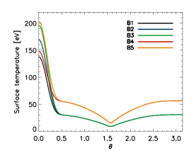
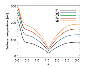
Given the theoretical uncertainties discussed above, it is not possible to make specific predictions for what the temperature distribution on the NS surfaces should be, and each case needs to be studied on its own. Therefore, for the general study of this work, we have opted to explore a variety of prescribed surface temperature profiles, without discussing their particular physical origin. In order to build them, we have used the most updated envelope models (used in Viganò et al. 2013 and adapted from Pons et al. 2009), with prescribed values of crustal temperature and magnetic field. In Fig. 1 we show some of the models studied in detail. The (un-redshifted) surface temperatures of all these models are in the typical range $\sim 10-300$ eV. For simplicity, we divide the models into three families. Family A, shown in the left panel, shows anisotropies qualitatively expected from neutron stars with crustal temperatures of $\sim 0.6-4\times 10^{8}$ K, and surface magnetic field $\sim 10^{13}$ G. Families B (middle) and C (right) add a small hot spot to models from A; such localized heated regions could have a variety of physical origins (i.e. particle bombardment, twisted magnetic bundles), as mentioned above.

3.2 Ray tracing and phase-dependent spectra

The general relativistic, phase-dependent spectra are calculated using the formalism developed by Page (1995). Due to light deflection by the gravitational field of the star, a photon emitted at an angle $\delta$ with the normal to the NS surface will reach the observer if generated at an angle (with respect to the viewing axis)

$$\theta_{v}(\delta)=\int_{0}^{\frac{R_{s}}{2R}}\,x\left[\left(1-{R_{s}\over R}\right)\left({R_{s}\over 2R}\right)^{2}-(1-2u)u^{2}x^{2}\right]^{-\frac{1}{2}}\,\mbox{d}u,$$ (1)

where $x\equiv\sin\delta$, $R_{s}\equiv 2GM/c^{2}$ is the Schwarzschild radius of the star, and $M$ and $R$ are its mass and radius, respectively. In this work, we employ $M=1.4M_{\odot}$ and $R=10$ km, yielding a gravitational redshift $(1-R_{s}/R)^{1/2}=0.766$. The radius measured by a distant observer would be $R_{\infty}=R/({1-{{R_{s}}/{R}}})^{1/2}=13$ km.

Table 2: Results from our synthetic phase-average spectra for an orthogonal rotator ($\chi=\xi=90^{\circ}$), considering the energy band 0.1–10 keV. We report the simulated number of photons, the best-fit parameters, 1-$\sigma$ errors, and $\chi_{\nu}^{2}$ values for the (absorbed, phabs) BB+line (bbodyrad*gabs) model. We also show the comparison with the best-fit BB model, the related $F$-test, the value of $N_{H}$ used in the synthetic spectra, $N_{H}^{\rm syn}$, and the value inferred from the fit, $N_{H}^{\rm fit}$. Radius and temperatures are reported as seen from an observer at infinity, at contrast with the physical unredshifted surface temperatures of Fig. 1. Equally good fits are often obtained for a wide range of the Gaussian width, up to $\sigma\sim E_{0}$ ($E_{0}$ being the line centroid): $\sigma$ has been fixed to the minimum value for which a good fit is found. For consistency, no error on the equivalent width ($E_{w}$) has been provided, since it is very sensitive to the choice of $\sigma$. Note that, since we consider an orthogonal rotator, the shown values of PF represent the maximum value that each representative model can achieve for local isotropic emission.

model	counts	$N_{H}^{\rm syn}$	$N_{H}^{\rm fit}$	$kT_{bb}$	$R_{bb}$	$E_{0}$	$|E_{w}|$	$\sigma$	$\chi_{\nu,bb+line}^{2}$	$\chi_{\nu,bb}^{2}$	PF
	[$10^{3}$]	$10^{20}{\rm cm}^{-2}$	$10^{20}{\rm cm}^{-2}$	[eV]	[km]	[eV]	[eV]	[eV]			(%)
A1	150	-	-	$44.5\pm 0.5$	$9.8\pm 0.3$	$320\pm 20$	70	100	1.05	1.53	$3.2$
A2	160	-	-	$53.5\pm 0.4$	$9.7\pm 0.2$	$360\pm 30$	90	100	0.99	1.40	$3.1$
A3	170	-	-	$61.6\pm 0.2$	$9.5\pm 0.1$	$450\pm 30$	90	100	0.98	1.45	$3.0$
A4	190	-	-	$77.4\pm 0.5$	$9.6\pm 0.1$	$490\pm 20$	30	100	1.04	1.57	$2.8$
A5	150	-	-	$91\pm 1$	$9.8\pm 0.1$	$570\pm 40$	70	150	1.00	1.32	$2.8$
A6	180	-	-	$112\pm 1$	$10.1\pm 0.2$	$630\pm 50$	60	200	1.05	1.41	$2.7$
A7	120	-	-	$131\pm 1$	$10.2\pm 0.2$	$670\pm 50$	50	200	0.95	1.31	$2.6$
B1	30	-	-	$86\pm 1$	$1.39\pm 0.05$	$440\pm 30$	50	150	1.10	1.42	$90$
B2	40	-	-	$106\pm 1$	$1.4\pm 0.1$	$540\pm 30$	70	150	1.07	1.37	$94$
B2	210	1	$0.5\pm 0.1$	$111\pm 1$	$1.17\pm 0.04$	$670\pm 30$	50	150	1.01	1.48	$99$
B2	250	10	$9.0\pm 0.3$	$113\pm 1$	$1.09\pm 0.03$	$710\pm 30$	30	150	1.11	1.31	$100$
B3	50	-	-	$123\pm 1$	$1.4\pm 0.1$	$590\pm 30$	60	150	1.03	1.38	$96$
B4	30	1	$\lesssim 0.5$	$91\pm 1$	$1.7\pm 0.1$	$530\pm 30$	140	150	0.90	1.42	$60$
B4	30	1	1 (fixed)	$83\pm 1$	$2.7\pm 0.1$	$480\pm 20$	240	150	1.04	1.42	$60$
B4	70	5	$3.0\pm 0.2$	$98\pm 1$	$1.2\pm 0.1$	$620\pm 30$	90	150	1.04	1.52	$83$
B5	140	1	$\lesssim 0.5$	$132\pm 1$	$1.3\pm 0.1$	$690\pm 40$	30	150	1.07	1.30	$83$
B5	90	2	$0.8\pm 0.2$	$128\pm 2$	$1.4\pm 0.1$	$610\pm 40$	50	150	1.12	1.36	$89$
B5	140	5	$3.6\pm 0.2$	$128.6\pm 0.6$	$1.4\pm 0.1$	$620\pm 20$	60	150	0.99	1.30	$95$
C1	50	5	$3.8\pm 0.4$	$126\pm$ 2	$5.5\pm$0.4	$810\pm$20	400	250	1.34	2.68	$29$
C1	30	10	$7.6\pm 0.8$	$133\pm$ 3	$4.5\pm$0.5	$890\pm$30	380	250	1.12	1.87	$35$
C1	30	20	$14.5\pm 1.5$	$140\pm$ 3	$3.3\pm$0.3	$900\pm$20	250	200	1.13	1.50	$44$
C2	90	5	$3.8\pm 0.3$	$134\pm$ 1	$7.0\pm$0.1	$880\pm$30	160	200	1.18	2.01	$16$
C2	80	20	$16\pm 1$	$143\pm$ 3	$5.5\pm$0.4	$1020\pm 40$	180	250	1.23	1.52	$24$
C3	50	100	$78\pm 1$	$185\pm$ 2	$1.8\pm$ 0.1	$1560\pm$40	100	250	0.97	1.31	$58$
C4	180	5	$4.3\pm 0.2$	$145\pm 1$	$8.4\pm 0.2$	$870\pm 30$	80	200	1.03	1.55	$11$
C4	1000	50	$47\pm 1$	$152\pm 2$	$7.1\pm 0.5$	$1030\pm 20$	80	300	1.23	1.53	$25$
C4	640	70	$59\pm 1$	$168\pm 1$	$4.4\pm 0.1$	$1440\pm 40$	50	200	1.13	1.57	$29$
C4	330	100	$87\pm 1$	$172\pm 1$	$3.9\pm 0.1$	$1500\pm 30$	60	200	1.16	1.48	$34$

As the star rotates with angular velocity $\Omega(t)$, the observer measures the modulated photon flux

$$F(E_{\infty},\alpha)=\frac{E_{\infty}^{2}}{c^{2}h^{3}}\frac{R_{\infty}^{2}}{D^{2}}\;\int_{0}^{1}2x\int_{0}^{2\pi}I[\theta_{v}(x),\phi_{v},E]\,\mbox{d}\phi_{v}\mbox{d}x\,,$$ (2)

where $D$ is the distance, $E_{\infty}=E({1-{{R_{s}}/{R}}})^{1/2}$ is the energy measured by a distant observer, the spectral function $I(\theta_{v},\phi_{v},E)$ describes the dimensionless distribution of the locally emitted photons, and $(\theta_{v},\phi_{v})$ are the coordinates on the surface relative to the line of sight. Here we assume the local emission to be isotropic and corresponding to a blackbody distribution with temperature $T(\theta_{v},\phi_{v})$, i.e. $I=(e^{E/k_{B}T}-1)^{-1}$.

The temperature distributions are assumed to be axisymmetric (see Fig.1), and the magnetic axis is taken to coincide with the axis of symmetry of the temperature distribution. If we indicate by $\psi$ and $\xi$ the angles that the rotation axis makes respectively with the line of sight and the magnetic axis, then the angle between the line of sight and the magnetic axis, $\alpha$, is given by the simple geometric relation

$$\alpha(t)=\arccos\left[\cos\psi\cos\xi+\sin\psi\sin\xi\cos\gamma(t)\right]\,,$$ (3)

where $\gamma(t)=\int\Omega(t)dt$ is the phase angle swept by the star during its rotation (see Fig.1 in Perna & Gotthelf 2008 for a graphical representation of the viewing geometry). From Eq. (2), the phase-averaged spectrum can be readily computed as an integral over the phase angle $\gamma$. For simplicity, we focus our analysis on spectra computed with $\psi=\xi=90^{\circ}$ (orthogonal rotator), while briefly discussing the effects of the viewing geometry on the presented results.

Figure 3: Best fit parameters for BB+line model, applied to real data (black asterisks, see Table 1), and synthetic spectra of Table 2 (blue and red squares for models with $N_{H}=0$ and $N_{H}>0$, respectively). Top: correlation of $E_{0}/kT$ with $N_{H}$. Bottom: correlation between $E_{0}$ and $kT_{bb}$ (the hottest is considered in the case of real sources showing multi-T component).

4 Simulated Spectra and Fit Results

We imported the numerical, general relativistic spectra computed with the various temperature distributions into Xspec, as atable models. We then simulated synthetic observed spectra, using XMM-Newton/EPIC-pn response matrices in the fakeit procedure. For each model, we fixed the exposure time to be long enough to obtain a number of photons that would allow to detect possible spectral features.

Phenomenologically, the spectra of isolated NSs showing spectral lines in their thermal emission are typically fitted by a model composed of a thermal component (BB or atmosphere) plus a phenomenological absorption model (gabs, gauss, cyclabs in the fitting package Xspec, Arnaud 1996). When a phase-resolved spectral analysis is doable, spectral features can show phase-dependence (e.g., De Luca et al. 2004; Hambaryan et al. 2011; Kargaltsev et al. 2012).

For each simulated spectrum, we proceeded to the spectral analysis in the standard way, considering energies between 0.1–10 keV. We fitted the simulated spectra with two models: (a) BB, (b) BB+line (bbodyrad*gabs model in Xspec), with the Gaussian width, $\sigma$, fixed to a given value. Freezing $\sigma$ is a standard way to proceed also in real observations (see, e.g., Haberl et al. 2004b) when broad, weak features are present. As expected (see also Perna et al. 2013), the spectra from nearly uniform temperature distributions are always well fitted by a single BB. For conciseness, we do not discuss the trivial cases in detail. Hereafter we focus on the most interesting configurations for our purpose, i.e. those showing large temperature differences (at least a factor of $\sim$ 2) between the coldest and the hottest regions (see Fig. 1).

We evaluated the systematic improvement in the fits obtained with the BB+line model with respect to the pure BB, by looking at the shape of the residuals and the values of $\chi_{\nu}^{2}$ ($\chi^{2}$ normalized by the number of degrees of freedom) for the different realizations. We confirmed the robustness of the results by finding, for each model, the systematic appearance of a spurious line with similar parameters in tens of different simulations. By computing the contribution to the flux of lines and continuum, we can also estimate the equivalent width of the line, $E_{w}$. The latter, both in observations and in our simulations, is typically tens or hundreds of eV. However, note that equally good fits can often be found for similar values of $E_{0}$ but different values of $\sigma$ (varying by factor of a few), or different line models (gabs, gauss, cyclabs). Since this variability strongly affects the equivalent width, the values of the latter should be taken as an order-of-magnitude estimate. The results of the fits to a variety of simulated spectra are summarized in Table 2.

4.1 Phase-averaged spectra

We start by considering the representative case of the phase-averaged spectra for model B2, simulated with $N_{H}=10^{21}$ cm^-2. A pure BB fit gives an unacceptable $\chi_{\nu}^{2}$ and, more interestingly, it shows systematic residuals. The addition of a broad absorption line allows to better fit the data, at least by partly removing systematic residuals. In Fig. 2 we show the unfolded spectrum with the residuals coming from the best-fit BB+line model (removing the line for the sake of clarity), for a single realization of the synthetic spectrum.

Figure 4: Unfolded spectrum of RX J0806.4-4123, and best-fit (with residuals in units of $\chi_{\nu}$) for a BB+line model ($\chi_{\nu}^{2}=1.36$, shown in the upper panel, with the line removed), and a model ($\chi_{\nu}^{2}=1.18$, bottom panel) generated with an inhomogeneous temperature distribution.

The same qualitative behavior is seen in all the cases in which the BB+line model fits better than the BB. The basic requirement needed to create a feature in the spectrum is that the fluxes from the coldest and hottest parts of the star be comparable. In these cases, the spectral distribution, to first order, consists of two Planckian shapes, whose temperatures and emitting areas represent an average value of the coldest and hottest parts. The spectral feature appears in the energy range between the two Planckian peaks. The larger the difference in temperature, the deeper the feature.

In Table 2 we have collected the fit results from several model temperatures (among the ones explored) for which the spectral feature appears. This sample is not meant to be a complete and systematic exploration of the large space of possible temperature distributions, but only an illustration of some of the tested cases. For each of them, we show the best-fit parameters (with statistical errors) of the BB+line spectral model for a single realization, made with the indicated number of photons. In general, the central energy and the equivalent width are consistent with those observed in the considered sample.

In both the BB and the BB+line models, the inferred temperature $kT_{bb}$ corresponds to an average value of the redshifted surface temperatures (see also Perna et al. 2013). The values of $kT_{bb}$ for the BB and the BB+line models are compatible, while $R_{bb}$ can increase by up to $\sim 10\%$ in the BB+line case, in order to account for the flux absorbed by the line. An important point is that, in all the cases, a 2BB fit (with absorption, if needed) fits well the simulated data, as long as the counts are less than a few $\times 10^{5}$-$10^{6}$ (depending on the model), in which case further small deviations can be resolved.

In the models with $N_{H}=0$, we find spurious lines for the cases in which the majority of the surface is almost invisible though still able to contribute to the low-energy spectrum, $E\gtrsim 0.1$ keV. The same effect is obtained with hotter models but with large absorption, which again almost hides the cold component. In the case with absorption included, $N_{H}$ is left free to vary, and usually the best-fit absorbed BB (or BB+line) value underestimates the absorption column by $\sim 20$-$30\%$ with respect to the actual value used in the simulation. As a matter of fact, the single BB model tends to underestimate the flux coming from the colder part (which corresponds to a larger, colder region), thus needing less absorption to fit the data.

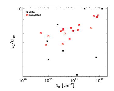
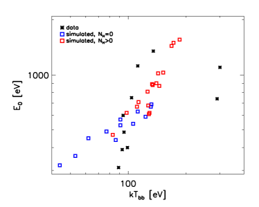
In Fig. 3 we show the correlation of $E_{0}/kT_{bb}$ with $N_{H}$ (left), and of $E_{0}$ with $kT_{bb}$ (right), both in real data (black) and in synthetic spectra (red). The spurious lines are centered at $E_{0}\sim 4$-$9~{}kT_{bb}$, corresponding to the tail of energy larger than the Wien peak of the spectrum given by the best-fit BB model. In observations, some of the lines lie in the same regions, while others are found at much larger energies, or much closer to the Wien peak. For those cases, this implies that the origin of the lines cannot be attributed to inhomogeneous surface temperatures.

Note also that selection effects limit the energy range in which lines can be found: solid claims cannot be made for $E_{0}$ close to the lower boundary of the energy domain. For large absorption, there are too few photons in the region of low energy (few hundreds of eV), and therefore no spectral details at low energy can be appreciated. The same applies to the upper region of Fig. 3 (left panel): thermal photons in that part are too few for any deviation from a single blackbody to be statistically significant. Low values of $N_{H}\lesssim 10^{20}$ cm^-2 slightly affect only the very low energy part of the spectrum, thus making $N_{H}$ poorly constrained and highly correlated with $kT_{bb}$ and $R_{bb}$ (see, for instance, two different fits for the model B4, with the same $N_{H}^{\rm syn}=10^{20}$ cm^-2 in Table 2).

In general, A-like models need a few $\times 10^{5}$ photons to make the line detectable, while many of the B and C models need only $3$-$5\times 10^{4}$ photons: the stronger the anisotropy, the easier it is to observe deviations from a pure BB, unless absorption is very large (see some of the C models). Another difference lies in the inferred radius from the fit ($R_{bb}$): while for the A models $R_{bb}$ is only slightly smaller than the radius of the star (seen at infinity, $R^{\infty}=13$ km), for the B and C models it is much smaller, corresponding to the size of the hot spot (see Fig. 1).

Last, we computed, for each representative model, the predicted pulsed fraction PF, defined as

$$PF=\frac{F_{\rm max}(\gamma)-F_{\rm min}(\gamma)}{F_{\rm max}(\gamma)+F_{\rm min}(\gamma)}\;,$$ (4)

where $F_{\rm max}$ and $F_{\rm min}$ are, respectively, the maximum and minimum flux as a function of phase in a given energy band. We selected the 0.1-2 keV band, above which the thermal flux becomes negligible for most models. All the models are computed for an orthogonal rotator ($\psi=\xi=90^{\circ}$), which yields the largest allowed value for the PFs for the considered emission model (blackbody). The observed PF of each source puts some constraints on the allowed range of angles, and this needs to be discussed case by case for specific objects. We will do so in the following section for the source RX J0806.4-4123.

Figure 5: Two possible temperature maps (single spot, with fit in Fig. 4, and double spot) that fit the phase-average spectrum of RX J0806.4-4123.

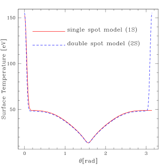
4.1.1 An example: fit to J0806.4-4123

In the previous subsection we have shown that the apparent lines in the simulated spectra have $E_{0}$ and $E_{w}$ values similar to the commonly observed ones. In the following we directly test our models for a particular source, J0806.4-4123. To this aim, we processed the 33.6 ks-long XMM–Newton/EPIC-pn observation of 2003 April 24^th, using SAS version 12, and employing the most updated calibration files.

Figure 6: PF map as a function of the angles $\psi$ and $\xi$ for the models 2S (top) and 1S (middle) of Fig. 5. Given the symmetry of the 2S model, a restricted parameter space is shown. For each model, the bottom panel shows two pulsed profiles, each computed for a choice of angles which yield pulsed fractions consistent with the observed value of $\sim 6\%$.

In the left panel of Fig. 4, we show the unfolded spectrum with the best-fit BB+line model ($\chi_{\nu}^{2}=1.36$) with $kT_{bb}=96$ eV, $E_{0}=486$ eV, $E_{w}=30$ eV, and $N_{H}$ unconstrained. The line has been removed in the plot for clarity. Several different temperature distributions (either with one or two hot spots) are able to fit the spectrum better than the BB model and the BB+line model. An example of one of such cases is shown in the right panel, with $N_{H}=(4.2\pm 0.1)\times 10^{20}$ cm^-2, $\chi_{\nu}^{2}=1.18$. Two of the typical temperature profiles that fit the data (symmetric/asymmetric distributions) are shown in Fig.  5.

Figure 7: Phase resolved spectra, for the model B2, without absorption. Left: $\chi_{\nu}^{2}$ of the best fitting BB (dashed) or BB+line model (solid) as a function of phase. Right: equivalent width, $E_{w}$, as a function of phase.

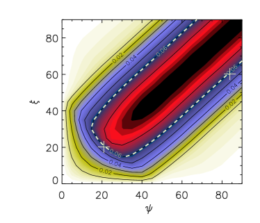
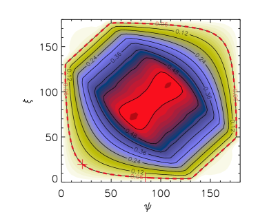
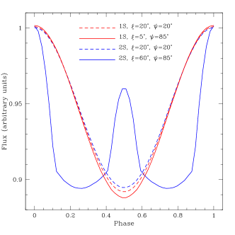
An independent, important constraint on the underlying temperature profile is provided by the pulsed profiles. For the XINSs, they are generally single-peaked, with relatively low pulsed fractions. In the particular case of the source J0806.4-4123, the PF in the EPIC-pn is $6\%$ in the 0.12-1.2 keV band (Haberl & Zavlin, 2002). We hence explored the parameter space in the angles $\psi,\xi$ which can yield this modulation level, for both models. We note that, without the effect of interstellar absorption, the modulation level of the models in a wide energy band is low, even for an orthogonal rotator ($\psi=\xi=90^{\circ}$). This is because, as already discussed, the models that yield spectral features are characterized by comparable fluxes in the hot and colder regions (dominant at opposite phases). However, for sources with high $N_{H}$, the colder component is largely absorbed, thus lowering the flux at the minimum of the pulsed profile and resulting in an increased PF in a wide band (see Perna et al. 2000 for an extensive discussion of this topic). This is particularly so for the single spot model.

Fig. 6 shows contour plots of the PF as a function of the angles $\psi,\xi$ for the two models used for the fit of J0806.4-4123 (Fig. 5). As expected, in each case there is a range of viewing angles which yield values of the PF consistent with the observed value of 6% (thick dashed line in the figure). In the single spot case, the profile is single peaked for all the choices along this degenerate region. On the other hand, for the double spot, some viewing geometries, even if consistent with the observed PF, can however be ruled out as they would yield a double peaked profile, unlike that observed. Among the range of angles yielding PF$\sim 6$%, we have selected, for the double spot, one particular choice of angles yielding a double peaked profile, and another yielding a single peaked one (favoured by the observations). The single peak profiles require solutions to be close to the main diagonal, with allowed angles in the range $\psi\approx\xi\approx 10^{\circ}-30^{\circ}$. On the other hand, solutions such as the one displayed with $\xi\approx 85^{\circ}$ and $\psi\approx 60^{\circ}$ would show a second (lower) maximum in the pulsed profile.

Finally, we should note that the derived values of the viewing angles should be taken with caution, for two reasons: first, here we have assumed blackbody, perfectly isotropic emission, and realistic atmospheres are known not to be such (e.g. Zavlin et al. 1996); second, a change of viewing angles implies, in turn, slighlty different phase-average spectra, and a non-trivial, iterative fine-tuning of both temperature distribution and viewing angles would be needed to achieve a fully consistent fit of all observed properties.

4.2 Phase-resolved analysis

The phase-resolved spectra strongly depend on the inclination and viewing angles. In axial symmetry, the most extreme phase-variability (and pulsed fraction, PF) is obtained when $\xi=\psi=90^{\circ}$ (orthogonal rotator). The smaller the angles, the less distinguishable in phase are the hot and cold regions, because all the hot spots/rings are seen in most phases.

We analyzed the fake phase-resolved spectra for model B2 with $\xi=\psi=90^{\circ}$, considering 20 different phase angles $\gamma$. Again, we fit with a BB model, with or without a gaussian absorption line with $\sigma$ fixed at 150 eV.

In Fig. 7, we plot $\chi_{\nu}^{2}$ and the value of $E_{w}$ as a function of density. The BB+line model fits significantly better than the BB for all the phases at which the northern hotspot is seen. On the other hand, around $\gamma=\pi$, the hotspot is not seen, the temperature distribution is more homogeneous, and a single blackbody fits well. The equivalent width remains constant in phase, until the hot spot goes out of sight, and $E_{w}$ approaches zero. When the spurious line is detected, its centroid, $E_{0}$, remains almost constant, within errors. On the other hand, models of family A show very little variability, because, being axisymmetric, at least one of the two hot poles is always seen.

Therefore, asymmetric temperature distributions are characterized by a strong phase variability in the equivalent width of the spurious line, while the line centroid is barely affected. While these phase-dependent properties may not be unique to spectral features due to temperature inhomogeneities, they should be kept in mind in the process of interpreting the origin of spectral features, case by case.

5 Discussion

We have computed synthetic X-ray spectra of NSs for several inhomogeneous surface temperature maps and found that, in some cases, the spectra present features compatible with broad absorption lines at a high significance level. The distinguishing characteristic of the temperature distributions leading to these spectral distortions is one or more hot, small regions with a temperature larger by at least a factor of about 1.5-2 than the average temperature of the rest of the surface. The hot spot(s) and the cold parts should give similar contribution to the flux; the poor sensitivity of the instruments at low energy and/or the interstellar absorption, partially hide the Planckian emission produced by the coldest regions. As a consequence, the spurious line appears between the two Planckian peaks. In light of our analysis, we propose that the need for absorption lines in the fits to some isolated neutron stars may be a hint for inhomogeneous temperature distributions, but the opposite is not generally true: an inhomogeneous temperature does not always imply the appearance of a spectral line. The NS in the SNR Kes79 (Halpern & Gotthelf, 2010) shows strong hints for anisotropy (two BBs in the spectral fits, and/or a large pulsed fraction), but it does not require a line in the spectrum.

In our synthetic models, the values of the line model parameters ($E_{0}$ and $E_{w}$) are in the same ranges as the observed ones. The spurious lines always appear beyond the Wien peak of the BB+line model, and $E_{0}\sim 4-9~{}kT_{bb}$. Most objects (e.g., XINSs and PSRs), show a similar position of $E_{0}$. However, conclusions cannot be drawn only on the basis of this property; rather, each object should be considered separately. As an example, we have performed a fit to RX J0806.4-4123, finding several different temperature distributions able to give acceptable fits, better than the BB+line fit. This shows that, at least for this object, a temperature inhomogeneity can produce deviations from a pure BB model similar to the observed ones. The gross features of On the other hand, other sources like CCO 1E1207.4-5209 and the XINSs RX J1308.6+2127 are cases for which the deviations from a BB spectrum do not appear to be reproducible by inhomogeneous temperature distributions. The exceptional spectral complexity of these sources cannot be mimicked, even qualitatively, by any of the many surface temperatures that we have tested.

In general, we remark that, given the wide space of parameters of the temperature modeling, reconstructing the surface temperature map is a highly degenerate problem. Moreover, for the purpose of isolating spectral effects due to temperature anisotropy alone, here we have used local blackbody emission rather than realistic, magnetized atmospheric/condensed surface models. These are the reasons for which we did not attempt individual fits to all the sources. Rather, we have demonstrated that the contribution to spectral features from inhomogeneous temperature distributions can be significant, and hence this should be accounted for in combination with more sophisticated emission models.

To conclude, we note that, while current observations still allow several interpretations for the observed absorption features, the very large effective area of the planned X-ray mission Athena+ (Nandra et al., 2013) will provide top-quality spectra, with the possibility of fine-tuning the spectral models and possibly discriminating between different underlying physical mechanisms.

References

- Albano et al. (2010) Albano A., et al., 2010, ApJ, 722, 788
- Arnaud (1996) Arnaud K. A., 1996, in Jacoby G. H., Barnes J., eds, Astronomical Data Analysis Software and Systems V Vol. 101 of Astronomical Society of the Pacific Conference Series, XSPEC: The First Ten Years. p. 17
- Becker (2009) Becker W., 2009, in Becker W., ed., Astrophysics and Space Science Library Vol. 357 of Astrophysics and Space Science Library, X-Ray Emission from Pulsars and Neutron Stars. p. 91
- Beloborodov (2013) Beloborodov A. M., 2013, ApJ, 777, 114
- Bernardini et al. (2009) Bernardini F., et al., 2009, A&A, 498, 195
- Bernardini et al. (2011) Bernardini F., et al., 2011, MNRAS, 418, 638
- Bignami et al. (2003) Bignami G. F., Caraveo P. A., De Luca A., Mereghetti S., 2003, Nature, 423, 725
- Burwitz et al. (2003) Burwitz V., et al., 2003, A&A, 399, 1109
- Chen et al. (1974) Chen H.-H., Ruderman M. A., Sutherland P. G., 1974, ApJ, 191, 473
- Cheng & Ruderman (1980) Cheng A. F., Ruderman M. A., 1980, ApJ, 235, 576
- De Luca et al. (2004) De Luca A., et al., 2004, A&A, 418, 625
- De Luca et al. (2005) De Luca A., et al., 2005, ApJ, 623, 1051
- de Luca et al. (2012) de Luca A., et al., 2012, MNRAS, 421, L72
- de Vries et al. (2004) de Vries C. P., et al., 2004, A&A, 415, L31
- Gotthelf et al. (2013) Gotthelf E. V., Halpern J. P., Alford J., 2013, ApJ, 765, 58
- Gotthelf et al. (2010) Gotthelf E. V., Perna R., Halpern J. P., 2010, ApJ, 724, 1316
- Haberl et al. (2003) Haberl F., et al., 2003, A&A, 403, L19
- Haberl et al. (2004a) Haberl F., et al., 2004a, A&A, 419, 1077
- Haberl et al. (2004b) Haberl F., et al., 2004b, A&A, 424, 635
- Haberl et al. (2006) Haberl F., et al., 2006, A&A, 451, L17
- Haberl & Zavlin (2002) Haberl F., Zavlin V. E., 2002, A&A, 391, 571
- Halpern & Gotthelf (2005) Halpern J. P., Gotthelf E. V., 2005, ApJ, 618, 874
- Halpern & Gotthelf (2010) Halpern J. P., Gotthelf E. V., 2010, ApJ, 709, 436
- Halpern & Ruderman (1993) Halpern J. P., Ruderman M., 1993, ApJ, 415, 286
- Hambaryan et al. (2011) Hambaryan V., et al., 2011, A&A, 534, A74
- Ho (2007) Ho W. C. G., 2007, MNRAS, 380, 71
- Ho et al. (2007) Ho W. C. G., et al., 2007, MNRAS, 375, 821
- Ho & Lai (2001) Ho W. C. G., Lai D., 2001, MNRAS, 327, 1081
- Ho & Lai (2003a) Ho W. C. G., Lai D., 2003a, in Hubeny I., Mihalas D., Werner K., eds, Stellar Atmosphere Modeling Vol. 288 of Astronomical Society of the Pacific Conference Series, Atmospheres and Spectra of Strongly Magnetized Neutron Stars. p. 621
- Ho & Lai (2003b) Ho W. C. G., Lai D., 2003b, MNRAS, 338, 233
- Ho et al. (2003) Ho W. C. G., Lai D., Potekhin A. Y., Chabrier G., 2003, ApJ, 599, 1293
- Hohle et al. (2012a) Hohle M. M., et al., 2012a, MNRAS, 419, 1525
- Hohle et al. (2012b) Hohle M. M., et al., 2012b, MNRAS, 423, 1194
- Ibrahim et al. (2003) Ibrahim A. I., Swank J. H., Parke W., 2003, ApJL, 584, L17
- Kaplan & van Kerkwijk (2009a) Kaplan D. L., van Kerkwijk M. H., 2009a, ApJ, 705, 798
- Kaplan & van Kerkwijk (2009b) Kaplan D. L., van Kerkwijk M. H., 2009b, ApJL, 692, L62
- Kaplan & van Kerkwijk (2011) Kaplan D. L., van Kerkwijk M. H., 2011, ApJL, 740, L30
- Kargaltsev et al. (2012) Kargaltsev O., et al., 2012, Science, 337, 946
- McLaughlin et al. (2007) McLaughlin M. A., et al., 2007, ApJ, 670, 1307
- Mereghetti (2008) Mereghetti S., 2008, A&ARv., 15, 225
- Miller et al. (2013) Miller J. J., et al., 2013, ApJ, 776, 104
- Miller (1992) Miller M. C., 1992, MNRAS, 255, 129
- Mori et al. (2005) Mori K., Chonko J. C., Hailey C. J., 2005, ApJ, 631, 1082
- Mori & Hailey (2006) Mori K., Hailey C. J., 2006, ApJ, 648, 1139
- Nandra et al. (2013) Nandra K., et al., 2013, arXiv:astro.ph/1306.2307
- Özel (2001) Özel F., 2001, ApJ, 563, 276
- Page (1995) Page D., 1995, ApJ, 442, 273
- Page et al. (2007) Page D., Geppert U., Küker M., 2007, Ap&SS, 308, 403
- Pavlov et al. (1995) Pavlov G. G., Shibanov Y. A., Zavlin V. E., Meyer R. D., 1995, in Alpar M. A., Kiziloglu U., van Paradijs J., eds, The Lives of the Neutron Stars Neutron Star Atmospheres. p. 71
- Pérez-Azorín et al. (2006) Pérez-Azorín et al., 2006, A&A, 459, 175
- Perna et al. (2013) Perna R., et al., 2013, MNRAS, 434, 2362
- Perna & Gotthelf (2008) Perna R., Gotthelf E. V., 2008, ApJ, 681, 522
- Perna et al. (2000) Perna R., Heyl J., Hernquist L., 2000, ApJL, 538, L159
- Pires et al. (2012) Pires A. M., et al., 2012, A&A, 544, A17
- Pires et al. (2014) Pires A. M., et al., 2014, A&A, 563, A50
- Pons et al. (2002) Pons J. A., et al., 2002, ApJ, 564, 981
- Pons et al. (2009) Pons J. A., Miralles J. A., Geppert U., 2009, A&A, 496, 207
- Rea et al. (2003) Rea N., et al., 2003, ApJL, 586, L65
- Rea et al. (2005) Rea N., et al., 2005, MNRAS, 361, 710
- Rea et al. (2008) Rea N., et al., 2008, ApJ, 686, 1245
- Romani (1987) Romani R. W., 1987, ApJ, 313, 718
- Sanwal et al. (2002) Sanwal D., et al., 2002, ApJL, 574, L61
- Sartore et al. (2012) Sartore N., et al., 2012, A&A, 541, A66
- Schwope et al. (2007) Schwope A. D., et al., 2007, Ap&SS, 308, 619
- Suleimanov et al. (2009) Suleimanov V., Potekhin A. Y., Werner K., 2009, A&A, 500, 891
- Suleimanov et al. (2010) Suleimanov V. F., Pavlov G. G., Werner K., 2010, ApJ, 714, 630
- Suleimanov et al. (2012) Suleimanov V. F., Pavlov G. G., Werner K., 2012, ApJ, 751, 15
- Tiengo et al. (2013) Tiengo A., et al., 2013, Nature, 500, 312
- Turolla (2009) Turolla R., 2009, in Becker W., ed., Astrophysics and Space Science Library Vol. 357 of Astrophysics and Space Science Library, Isolated Neutron Stars: The Challenge of Simplicity. p. 141
- van Adelsberg et al. (2005) van Adelsberg M., et al., 2005, ApJ, 628, 902
- van Adelsberg & Lai (2006) van Adelsberg M., Lai D., 2006, MNRAS, 373, 1495
- van Kerkwijk et al. (2004) van Kerkwijk M. H., et al., 2004, ApJ, 608, 432
- van Riper (1988) van Riper K. A., 1988, ApJ, 329, 339
- Viganò et al. (2013) Viganò D., et al., 2013, MNRAS, 434, 123
- Zane et al. (2005) Zane S., et al., 2005, ApJ, 627, 397
- Zavlin & Pavlov (2004) Zavlin V. E., Pavlov G. G., 2004, ApJ, 616, 452
- Zavlin et al. (1996) Zavlin V. E., Pavlov G. G., Shibanov Y. A., 1996, A&A, 315, 141
- Zavlin et al. (1998) Zavlin V. E., Pavlov G. G., Trumper J., 1998, A&A, 331, 821