Interacting Weyl semimetals: characterization via the topological Hamiltonian
and its breakdown

Abstract

Weyl semimetals (WSMs) constitute a 3D phase with linearly-dispersing Weyl excitations at low energy, which lead to unusual electrodynamic responses and open Fermi arcs on boundaries. We derive a simple criterion to identify and characterize WSMs in an interacting setting using the exact electronic Green’s function at zero frequency, which defines a topological Bloch Hamiltonian. We apply this criterion by numerically analyzing, via cluster and other methods, interacting lattice models with and without time-reversal symmetry. We identify various mechanisms for how interactions move and renormalize Weyl fermions. Our methods remain valid in the presence of long-ranged Coulomb repulsion. Finally, we introduce a WSM-like phase for which our criterion breaks down due to fractionalization: the charge-carrying Weyl quasiparticles are orthogonal to the electron.

The emergence of (quasi)relativistic excitations in quantum condensed matter has stimulated much theoretical and experimental research, especially following the discoveries of grapheneGeim and Novoselov (2007); Castro Neto et al. (2009) and 3D topological insulatorsHasan and Kane (2010); Qi and Zhang (2011), both of which host 2D massless Dirac fermions. More recently, a 3D analog of graphene, the Weyl semimetal (WSM), has piqued physicists’ curiosity, partially due to its potential for realization in transition metal oxides with strong interactions and spin-orbit couplingWan et al. (2011); Xu et al. (2011); Witczak-Krempa and Kim (2012); Witczak-Krempa et al. (2014), or heterostructuresBurkov and Balents (2011). Such a phase has stable massless Weyl quasiparticles, which can be viewed as half-Dirac fermions. These lead to unique open Fermi arc surface statesWan et al. (2011) and electromagnetic responsesNielsen and Ninomiya (1983); Haldane (2004); Yang et al. (2011); Turner and Vishwanath (2013); Vafek and Vishwanath (2014); Parameswaran et al. (2014); Hosur (2012); Potter et al. (2014); Panfilov et al. (2014). Such properties rely on the topological nature of the Weyl pointsVolovik (2003), which are monopoles of the non-interacting Berry curvature. As WSMs naturally arise in interacting lattice modelsTurner and Vishwanath (2013); Witczak-Krempa et al. (2014); Vafek and Vishwanath (2014), it is important to characterize them without relying on free-electron or field-theoretic approachesGo et al. (2012); Wang and Zhang (2012a); Mastropietro (2013); Sekine and Nomura (2013), neither of which is sufficient to provide accurate predictions for most realistic systems. Moreover, an efficient method for searching for Weyl points in the interacting setting is desired because they generally occur at incommensurate points in the Brillouin Zone (BZ), often due to spontaneous symmetry breaking.

We provide a simple criterion to identify and characterize WSMs in the quantum many-body setting based on the electronic lattice Green’s function. Specifically, we use an effective Bloch Hamiltonian (dubbed “topological Hamiltonian”) defined from the zero-frequency many-body Green’s function, and argue that its eigenstates retain the Berry phase properties of the Weyl nodes. This allows for the extraction of the non-trivial surface statesWan et al. (2011) and anomalous quantum Hall (AQH) responseHaldane (2004); Yang et al. (2011) of interacting WSMs. We apply our results in conjunction with Cluster Perturbation TheorySénéchal et al. (2000) to study the physics of two interacting lattice models for WSMs, unraveling diverse interaction effects on the renormalization of the Weyl points. We also discuss the effects of long-range Coulomb repulsion which marginally destroys the quasiparticlesAbrikosov and Beneslavskii (1971), and argue that our approach remains valid in that case. Finally, we provide an instance where such methods break down due to a simple fractionalization into an orthogonalNandkishore et al. (2012) WSM. Our analysis naturally relates to previous works that characterized interacting topological insulators Wang et al. (2012); Wang and Zhang (2012b); Go et al. (2012); Hung et al. (2013); Lang et al. (2013); Deng et al. (2013); Laubach et al. (2013); Grandi et al. (2014) by means of the many-body Green’s function and associated Berry curvature, but differs in the sense that we study gapless systems.

Characterizing interacting Weyl semimetals: Non-interacting WSMs have a Fermi surface consisting of a finite number of points in the BZ, at which 2 bands meet linearly. Each such Weyl point can be identified with a hedgehog singularity of the Berry curvature, $\nabla\times{\bm{a}}({\bm{k}})$, i.e. a monopole of this $k$-space “magnetic” field. Here, ${\bm{a}}$ is the Berry connection defined via the occupied Bloch states. Knowledge of this monopole structure naturally leads to a description of the unusual open Fermi arc surface statesWan et al. (2011), and AQH responseHaldane (2004); Yang et al. (2011). In the presence of interactions that inevitably arise in realistic systems, the above band structure description no longer applies. However, we demonstrate that the essential features of the WSM remain robust, and can be understood in terms of the zero-frequency Green’s function.

We focus on short range interactions, while the effects of the long-ranged Coulomb repulsion are discussed towards the end. The central tool in our analysis is the imaginary-frequency Green’s function, $G(i\omega,{\bm{k}})$. It is a matrix in spin/orbital/sublattice space, and ${\bm{k}}$ belongs to the BZ of the lattice of the interacting system. A key observation is that one can define a many-body Berry connection ${\bm{\mathcal{A}}}({\bm{k}})$, and associated Berry curvature $\nabla\times{\bm{\mathcal{A}}}$, using the zero-frequency Green’s function. One begins by defining the so-called topological Hamiltonian:

$$\mathcal{H}_{t}({\bm{k}})=-G(0,{\bm{k}})^{-1}=\mathcal{H}({\bm{k}})+\Sigma(0,{\bm{k}})\,,$$ (1)

where $\mathcal{H}$ is the Bloch Hamiltonian of the non-interacting system, while $\Sigma(i\omega,{\bm{k}})$ is the exact self-energy matrix. $\mathcal{H}_{t}$ plays the role of an effective Bloch Hamiltonian: its eigenstates can be loosely viewed as substitutes of the Bloch states of the non-interacting system. The many-body Berry connection can then be introduced in exact analogy with non-interacting systems: ${\bm{\mathcal{A}}}({\bm{k}})=-i\sum_{\rm R-zeros}\langle n{\bm{k}}|\nabla|n{\bm{k}}\rangle\,,$ where $\mathcal{H}_{t}({\bm{k}})|n{\bm{k}}\rangle=\tilde{\xi}_{n}({\bm{k}})|n{\bm{k}}\rangle$ and $\{\tilde{\xi}_{n}({\bm{k}})\}$ defines the band structure of $\mathcal{H}_{t}$. R-zeroWang et al. (2012) signifies an eigenstate with $\tilde{\xi}_{n}({\bm{k}})\leq 0$. In the non-interacting limit, R-zeros reduce to occupied states, and ${\bm{\mathcal{A}}}$ to ${\bm{a}}$. We now argue that Weyl points of the interacting system can then be identified with monopoles of $\nabla\times{\bm{\mathcal{A}}}$ (analogously for higher charge monopolesFang et al. (2012)). An equivalent but more practical criterion follows: an interacting system is a WSM if the band structure of the topological Hamiltonian $\mathcal{H}_{t}$ has Weyl nodes at the Fermi level, which identify the Weyl nodes of the interacting system.

To understand the above criterion, let us consider a non-interacting WSM for which short-ranged interactions (attractive or repulsive) are adiabatically turned on. The latter are irrelevant in the renormalization group sense, i.e. at low energy, and one thus obtains a Weyl liquid, where excitations have an infinite lifetime only on the Fermi surface, i.e. at the Weyl nodes. By adiabacity, the monopole structure of the non-interacting Green’s function cannot be destroyed in the Weyl liquid. The many-body Berry connection ${\bm{\mathcal{A}}}$ captures the monopole of Berry fluxWang and Zhang (2012a) associated with the Weyl quasiparticles. This relates to Haldane’s statementHaldane (2004) about using the Berry curvature of the quasiparticles of a Fermi liquid to determine its AQH response (which translates to our expression for the latter, Eq. (2), being valid in that case), as one can approach a Weyl liquid from its parent Fermi liquid by tuning the doping.

We now support the above arguments by deriving the AQH response of a WSM in terms of the generalized Berry curvature ${\bm{\mathcal{A}}}$. We proceed by evaluating the many-body Chern number for 2D surfaces away from the Weyl points in the BZ.Wang and Zhang (2012a) More precisely, we will show that the anomalous part of the Hall conductivity reads:

$$\sigma_{ab}=\frac{e^{2}}{2\pi h}\epsilon_{abc}K^{c}\,;\qquad{\bm{K}}=\int_{\rm BZ}\frac{d^{3}{\bm{k}}}{2\pi}\,\nabla\times{\bm{\mathcal{A}}}({\bm{k}})\,,$$ (2)

where $\epsilon_{abc}$ is the Levi-Civita tensor. Eq. (2) generalizes the non-interacting formulaHaldane (2004), and can be collapsed to Fermi surface data: ${\bm{K}}=\sum_{m}q_{m}{\bm{k}}_{m}$, where ${\bm{k}}_{m}$ is a Weyl node of the interacting system, and $q_{m}=\pm 1$, its monopole charge. Eq. (2) can be deduced by starting with the frequency-dependent Green’s function. For simplicity, we consider a fixed $k_{x}$ away from the Fermi surface of the interacting WSM. It follows that $G(i\omega,{\bm{k}})$ defines a gapped 2D Green’s function in the $k_{y,z}$ plane. We can compute the many-body Chern number associated with $G$ at fixed $k_{x}$So (1985); Ishikawa and Matsuyama (1986):

$$\!\!\!\!C_{x}(k_{x})\!=\!\!\int\!\!\frac{d\omega d{\bm{k}}_{y,z}}{24\pi^{2}}\epsilon_{\mu\nu\rho x}\!\operatorname{Tr}G\partial_{\mu}G^{-1}G\partial_{\nu}G^{-1}G\partial_{\rho}G^{-1}$$ (3)

The $x$-component of the anomalous Hall vector is then the integral over the Chern number: $K_{x}=\int dk_{x}C_{x}(k_{x})$. We note that this latter expression agrees with the so-called Adler-Bell-Jackiw anomaly coefficient of the current correlator (see Appendix A). Now, to recover Eq. (2), we adiabatically deform the interacting Green’s function into the topological Green’s function, $G_{t}(i\omega,{\bm{k}})^{-1}=i\omega-\mathcal{H}_{t}({\bm{k}})$, via the interpolation: $g_{\lambda}(i\omega,{\bm{k}})=(1-\lambda)G(i\omega,{\bm{k}})+\lambda G_{t}(i\omega,{\bm{k}})$, $0\leq\lambda\leq 1$. Indeed, for any slice away from the Fermi surface, the gap of $g_{\lambda}$ remains open during the protocol since $g_{\lambda}(0,{\bm{k}})=G(0,{\bm{k}})$ for all $\lambda$. Further, $g_{\lambda}(i\omega,{\bm{k}})$ does not have zero eigenvaluesWang and Zhang (2012b). Thus, the many-body Chern number cannot change as $\lambda$ varies from 0 to 1, being a topological index, and we can use $g_{\lambda=1}=G_{t}(i\omega,{\bm{k}})$ to compute $C_{x}$. The frequency integral then yields Eq. (2) (Appendix A).

Using topological Hamiltonians numerically: We study two lattice models of interacting WSMs numerically to show the usefulness of the topological Hamiltonian approach. We identify and explain the motion and renormalization of the Weyl points as a function of the interaction strength. We consider Hubbard models:

$$H=H_{0}+U\sum_{r}n_{r,\uparrow}n_{r,\downarrow}-\mu\sum_{r,\sigma}n_{r,\sigma}\,,$$ (4)

where $H_{0}$ is a tight-binding hopping Hamiltonian of spin-1/2 electrons, which are created at site $r$ by $c_{r,\sigma}^{\dagger}$, and their number density per spin projection is $n_{r,\sigma}=c_{r,\sigma}^{\dagger}c_{r,\sigma}$. $U$ is the Hubbard interaction parameter; we consider both the attractive and repulsive cases. We study models that are defined on the cubic lattice, have particle-hole symmetry and are WSMs at the non-interacting level, and fix the chemical potential at the nodes, $\mu=U/2$.

Model I breaks time-reversal and is defined byYang et al. (2011):

$$\!\!\!H_{0}\!=\!\sum_{{\bm{k}}}c_{{\bm{k}}}^{\dagger}\big{[}\{2t(\cos k_{x}-\cos k_{0})+m(2-\cos k_{y}-\cos k_{z})\}\sigma_{x}\\ +2t\sin k_{y}\,\sigma_{y}+2t\sin k_{z}\,\sigma_{z}\big{]}c_{{\bm{k}}}\,,$$ (5)

where the spacing of the cubic lattice has been set to unity, and the fermion operators are vectors in spin space. The Pauli matrices $\sigma_{a}$ act on the latter. Below we set $t=1$. Depending on the parameters $k_{0}$ and $m$, $H_{0}$ can have 2, 6 or 8 Weyl nodes. We focus on the regime where it only has 2 nodes, located on the BZ boundary at ${\bm{k}}=\pm(k_{0},0,0)$. See Fig. 1a for the $U=0$ band structure (recall that in that limit $\mathcal{H}_{t}=\mathcal{H}$). The anomalous Hall vector is thus given by ${\bm{K}}=2k_{0}\hat{x}$, i.e. $\sigma_{yz}=(e^{2}/2\pi h)2k_{0}$.

We now turn to the study of the interacting Hamiltonian using Cluster Perturbation TheorySénéchal et al. (2000) (CPT). This method, which is related to Dynamical Mean Field Theory, allows for an efficient numerical analysis. In essence, one first decomposes the periodic system into clusters with $N_{c}$ sites. Exact diagonalization is used to obtain the exact cluster Green’s function. The Green’s function of the lattice system is then obtained via strong-coupling perturbation theory. CPT becomes exact in the limit $U\rightarrow 0$ and at strong coupling, $U\rightarrow\infty$; it is controlled in the sense that convergence can be monitored with increasing the cluster size. We emphasize that it is not perturbative in $U$. See Appendix B for more details.

CPT allows a direct evaluation of the topological Hamiltonian $\mathcal{H}_{t}$, so that we can easily track the location of the Weyl points of the interacting system as a function of $U$. The results we present are for clusters of size $N_{c}=2^{3}$, at which point reasonable convergence with $N_{c}$ has been achieved (see Appendix B for further information regarding the convergence). A further increase of $N_{c}$ would not affect our conclusions. We set $m=3/2$, and $k_{0}=3\pi/8$. The positive band of the topological Hamiltonian is shown in Fig. 1a for a cut through the BZ and for different $U$ values. With increasing $U>0$, the Weyl points move to larger magnitude of the wave vector. This directly corresponds to an increase of the Hall conductivity $\sigma_{yz}$, Eq. (2), as shown in Fig. 1b. The red circles are evaluated numerically with CPT. We also show the analytic strong coupling result (perturbative in $1/U$; derived in Appendix C), i.e. for single-site clusters, which captures the overall trend. For attractive interactions $U<0$, the trend is opposite: the Weyl points move towards ${\bm{k}}=0$. One can understand this heuristically: a positive/negative $U$ enhances/reduces the ferromagnetic moment $\langle c_{r}^{\dagger}\sigma_{x}c_{r}\rangle$ (already present at $U=0$), thus enhancing/reducing the Hall conductivity. A crude estimate of this effect can be obtained using mean field theory (Appendix C), as shown in Fig. 1b.

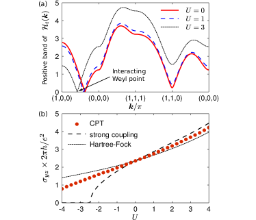
Figure 1: a) Positive band of the topological Hamiltonian $\mathcal{H}_{t}=-G(0,{\bm{k}})^{-1}$ of model I with varying interaction strength $U$ along a cut through the BZ. b) The Weyl points move with varying $U$, altering the Hall conductivity $\sigma_{yz}$. Filled circles come from the numerical simulations. $\sigma_{yz}$ in the strong/weak coupling limit is shown (dashed/dotted line). The numerical results are obtained with Cluster Perturbation Theory for a cluster of size $N_{c}=2^{3}$; the single-particle Hamiltonian has $m=3/2,\,k_{0}=3\pi/8$.

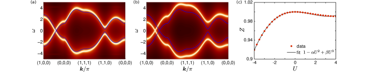
Figure 2: Density plot of the single particle spectral function $A(\omega,{\bm{k}})$ for a) $U=1$, b) $U=3$ obtained via CPT, shown on a logarithmic color scale. The non-interacting band structure (solid blue line) is the same as in Fig. 1. c) Dependence of the residue $Z$ of the Weyl quasiparticles on $U$; it is well approximated by a cubic polynomial.

In studying the Weyl points and AQH response of the many-body system, the topological Hamiltonian allowed a streamlined analysis by circumventing the need for the full frequency-dependent Green’s function. We now discuss some of the properties arising from the latter but not captured by $\mathcal{H}_{t}$. The spectral function $A(\omega,{\bm{k}})=-\operatorname{Tr}\operatorname{Im}G_{R}(\omega+i0^{+},{\bm{k}})/\pi$ obtained using CPT for $U\geq 0$ is shown in Fig. 2. The linearly dispersing Weyl modes can clearly be seen. In the interacting WSM only the excitations at the Weyl points remain sharp. The scattering rate of an excitation with momentum exactly at a Weyl point and with small frequency vanishes like $|\omega|^{5}$, as can be obtained perturbatively as shown in Appendix D. This is smaller than the Fermi liquid result $\omega^{2}$, owing to the vanishing density of states at the Fermi level in a WSM. As in a FL, the weight of the quasiparticles $Z$ will be reduced with increasing interactions. (When the Weyl nodes are related by symmetry they share the same $Z$, which is the case in this work.) The result is plotted in Fig. 2c, and as expected behaves as $Z\approx 1-\alpha U^{2}$ at small $U$, $\alpha>0$.

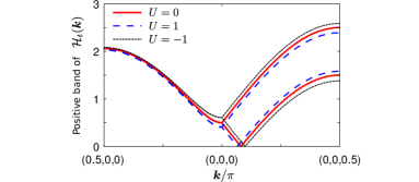
Figure 3: Positive band of the topological Hamiltonian $\mathcal{H}_{t}$ of model II ($\epsilon=0.5$) with varying Hubbard $U$ along a cut through the BZ. $U=0$ is the non-interacting band structure.

We introduce a new model which, in contrast to model I, preserves TRS but not inversion, and as such is a representative of the second family of WSMs. We show that the influence of interactions on the motion of the Weyl points has an altogether different physical origin as compared to model I, but a connection can be made by interchanging the role of magnetic and charge orders. The tight-binding Hamiltonian of model II reads:

$$\!H_{0}\!=2t\!\sum_{{\bm{k}},b=x,y,z}\!c_{{\bm{k}}}^{\dagger}\,\sigma_{b}\sin k_{b}\,c_{{\bm{k}}}+\epsilon H_{\rm cdw}\,,$$ (6)

where $H_{\rm cdw}$ corresponds to a $(\pi,\pi,0)$ charge density wave (CDW) on the cubic lattice where the chemical potential is staggered by $\pm\epsilon$ in a checkerboard fashion in the $xy$ plane. When $\epsilon=0$, we do not expect the 8 Weyl points to move under the effect of interactions (modulo possible instabilitiesMaciejko and Nandkishore (2013) beyond a critical $U$) because they are located at special high-symmetry $k$-points. The CPT calculation corroborates this. We thus need to turn on a finite $\epsilon$ to get non-trivial evolution. At $U=0$, we find a total of 16 Weyl points when $|\epsilon|<1$, setting $t=1$. (Going from 8 to 16 Weyl points as $\epsilon$ is turned on does not violate the indivisible nature of Weyl points since the CDW changes the BZ.) When $\epsilon=0$, four Weyl points occur at $k_{z}=0$, while four other ones at $\pi/a$, where we have reinstated the spacing of the original cubic lattice $a$. When $0<\epsilon<1$, the eight nodes at $k_{z}=0$ “split” to ones at $k_{z}a=\pm\sin^{-1}(\epsilon/2)$, similarly for $k_{z}=\pi/a$. A finite $U$ moves the eight nodes nearest to $k_{z}=0$ towards/away from $k_{z}=0$ since a repulsive/attractive $U$ disfavors/favors the charge imbalance. This is confirmed by Fig. 3, which shows $\mathcal{H}_{t}$ obtained using CPT.

Long-ranged Coulomb interaction: We have so far limited our discussion to short-ranged interactions. However, in an electronic WSM the screening of the Coulomb interaction is weak due to the vanishing density of states at the Fermi energy. Using RPA, it was shownAbrikosov and Beneslavskii (1971) that for linearly dispersing electrons in 3D interacting via an instantaneous Coulomb $1/r$ repulsion, the quasiparticle at the node ${\bm{k}}_{0}$ is marginally destroyed: $\operatorname{Im}\Sigma_{R}(\omega+i0^{+},{\bm{k}}_{0})\sim|\omega|$, resulting in a “marginal Weyl liquid”. Notwithstanding, this does not alter the fundamental Berry curvature structure around the (marginal) Weyl point. Indeed, let us consider the low-energy description near such an isotropic point: $\mathcal{H}_{t}({\bm{k}})=-G(0,{\bm{k}})^{-1}=f(k){\bm{k}}\cdot{\bm{\sigma}}$, where $f=1+\lambda\ln(\Lambda/k)$Abrikosov and Beneslavskii (1971). Crucially, the Berry curvature $\nabla\times{\bm{\mathcal{A}}}$ is independent of the overall real renormalization factor $f$ as it measures the complex phase of the $G$ eigenstates as they are parallel transported in the BZ. Thus, the Berry flux through a small sphere surrounding the Weyl point will measure the same monopole charge as when $f\equiv 1$. An analogous statement can be made about the $\pi$ Berry phase of the Dirac points of graphene in the presence of Coulomb repulsion.

Orthogonal Weyl semimetals: We present a case where the above characterization of a Weyl-like liquid using $\mathcal{H}_{t}$ breaks down. The idea being that particular interactions can induce a phase where the charge carrying quasiparticles have the properties of a WSM but are orthogonal to the electron due to fractionalization. Such a phase admits a simple and stable slave-particle description: the electron operator $c_{r,\sigma}$ can be written as the product $f_{r,\sigma}\tau_{r}^{x}$ of a slave fermion $f_{r,\sigma}$ carrying the charge (and spin), and a slave Ising pseudospin $\tau_{r}^{x}$. A $\mathbb{Z}_{2}$ gauge redundancy emerges because of the decomposition. In terms of these slave operators, a WSM results when the $f$-fermions form a WSM while the pseudospins are ordered. However, if they become disordered, an orthogonal WSM results for the electrons: The $f$-fermions constitute a Weyl liquid since the pseudospins and $\mathbb{Z}_{2}$ gauge field are gapped, but they are orthogonal to the electrons (the electronic quasiparticle weight vanishes). The resulting orthogonal WSM is a cousin phase of the orthogonal metalNandkishore et al. (2012). It has qualitatively the same thermodynamic and transportHosur and Qi (2013); Lundgren et al. (2014) properties as a Weyl liquid: $T^{3}$ heat capacity, quantum oscillationsPotter et al. (2014) and AQH response. However, the electron Green’s function $G$ shows a hard “Mott” gap, thus no Weyl points. In this sense, the AQH response can no longer be obtained using $\mathcal{H}_{t}=-G(0,{\bm{k}})^{-1}$. Instead, one has to use the $f$-fermion Green’s function. We thus have an instance where the adiabaticity relation to bare electrons breaks down, but where the topological Hamiltonian approach can be adapted by identifying the low-energy excitations. A similar situation will arise for other orthogonal states, such as orthogonal topological insulatorsMaciejko et al. (2014).

Conclusion: We have shown how to characterize interacting WSMs via the many-body Berry curvature (derived from the zero-frequency Green’s function) allowing the identification of the monopole structure of the Weyl points. We have argued that the existence of quasiparticles is not necessary in this, for example the latter are marginally destroyed in a WSM with long-ranged Coulomb repulsion. As a natural extension, we note that $\mathcal{H}_{t}$ can also be used to efficiently identify Weyl nodes lying away from the Fermi surface, for example in a doped Weyl semimetal, which proves much simpler than resolving the full spectral function. In closing, our work shows the importance of the Berry connection derived from the Green’s function in the study of correlated fermions, especially their robust (quasi)topological features, in the gapless regime. We have illustrated that these ideas can be implemented numerically to study realistic models.

Acknowledgments: WWK is particularly indebted to D.M. Haldane, Y.B. Kim, S.S. Lee and T. Senthil for discussions. We acknowledge stimulating exchanges with A. Go, B.I. Halperin, J. Maciejko, E.G. Moon, R. Nandkishore, A. Vishwanath. WWK is grateful for the hospitality of Harvard and the Princeton Center for Theoretical Physics, where some of the work was completed. MK was supported by the Austrian Science Fund (FWF) Project No. J 3361-N20. Research at Perimeter Institute is supported by the Government of Canada through Industry Canada and by the Province of Ontario through the Ministry of Research and Innovation.

Appendix A Anomalous quantum Hall conductivity via Green’s functions and Berry curvature

A.1 Green’s function expression for anomalous Hall conductivity

To obtain the AQH conductivity $\sigma_{ab}$, we use the Kubo formula. The time-reversal odd part of the current two-point (polarization) function that is relevant for $\sigma_{ab}$ reads:

$$\Pi_{ab}(q)=\frac{1}{(2\pi)^{2}}\epsilon_{ab\rho\lambda}q^{\rho}K^{\lambda}+\cdots\,,$$ (7)

where $(\cdots)$ refers to terms unimportant for the DC AQH response. The Roman/Greek indices run over spatial/spacetime dimensions. In contrast to the rest of the paper, we use real time and frequency in this subsection. Note that we have not assumed Lorentz invariance in Eq. (7); rather the above form is dictated by current conservation, which implies $q^{\mu}\Pi_{\mu\nu}(q)=q^{\nu}\Pi_{\mu\nu}(q)=0$. We have set $e=\hbar=1$; the later choice explains the extra factor of $1/2\pi$ compared to Eq. (2) of the main text. $q=(q^{0},{\bm{q}})$ is a four-momentum corresponding to the external electromagnetic perturbation, and $K^{\lambda}$ is a $q$-independent four-vector. In the Kubo formula for the conductivity, $\sigma_{ab}=\lim_{q^{0}\rightarrow 0}\lim_{{\bm{q}}\rightarrow{\bm{0}}}\Pi_{ab}(q)/q^{0}$, we first need to take the limit ${\bm{q}}={\bm{0}}$. We can thus set ${\bm{q}}={\bm{0}}$ in the above, which fixes the index $\rho=0$. Further, we can assume without loss of generality that ${\bm{K}}=(K_{x},0,0)$ is along the $x$-direction. We thus obtain

$$\sigma_{yz}=\frac{K_{x}}{(2\pi)^{2}}=\frac{\partial}{\partial q^{0}}\Pi_{yz}(q^{0},{\bm{0}})\big{|}_{q^{0}\rightarrow 0}\,.$$ (8)

Now, the exact polarization function reads

$$\Pi_{yz}(q)=\int\frac{dk^{0}d{\bm{k}}}{(2\pi)^{4}}\operatorname{Tr}\left[\Gamma_{y}^{(0)}(k,k+q)G(k+q)\Gamma_{z}(k+q,k)G(k)\right]\,,$$ (9)

where $\Gamma_{c}/\Gamma_{c}^{(0)}$ denotes the irreducible vertex function of the interacting/non-interacting theory. ($\Gamma_{\mu}(k,k^{\prime})$ has incoming fermion energy-momentum $k$, and outgoing one $k^{\prime}$.) Taking the frequency-derivative of Eq. (9), and using the Ward identityEngelsberg and Schrieffer (1963); Mahan (2000) associated with charge conservation (which is valid on the lattice),

$$\Gamma_{\mu}(k,k)=\partial_{\mu}G(k)^{-1}\,,$$ (10)

leads to the desired result for the anomalous quantum Hall response $\sigma_{yz}$:

$$\sigma_{yz}=\frac{1}{96\pi^{4}}\int_{-\infty}^{\infty}d\omega\int d{\bm{k}}\;\epsilon_{\mu\nu\rho x}\operatorname{Tr}[G(\partial_{\mu}G^{-1})G(\partial_{\nu}G^{-1})G(\partial_{\rho}G^{-1})]\,,$$ (11)

where we are using $e=\hbar=1$. The corresponding “triangle” Feynman diagram is shown in Fig. 4, where the external legs are at zero energy and momentum. The frequency derivative of the polarization function inserts an external photon line, leaving behind a three-point function. We note that the above formal manipulations are an extension to 3+1D of the corresponding ones in 2+1D used to obtain the quantized Hall conductivity of an interacting quantum Hall stateSo (1985); Ishikawa and Matsuyama (1986) using the exact Green’s function. The result was anticipated in Ref. Haldane, 2004 for Fermi liquids. In fact, the above derivation is general, and not specific to interacting WSMs.

It is straightforward to obtain Eq. (11) for a system of free-fermions, starting with the Kubo formula, Eq. (8). Indeed, minimal coupling the fermions to an external vector potential ${\bm{A}}$, $\mathcal{H}({\bm{k}})\rightarrow\mathcal{H}({\bm{k}}+{\bm{A}})$, gives the following expression for the spatial vertices: $\Gamma_{c}(k,k)=-\partial_{c}\mathcal{H}({\bm{k}})$. The time (or energy) component of the vertex is simply the identity matrix, $\Gamma_{0}(k,k)=1$, because the scalar potential $A_{0}$ couples to the fermion density. Note that the vertex function satisfies the Ward identity Eq. (10), where $G(k)^{-1}=k^{0}-\mathcal{H}({\bm{k}})$.

A.2 From Green’s functions to Berry curvature

Figure 4: Adler-Bell-Jackiw anomaly type Feynman diagram used to evaluate the DC anomalous quantum Hall response, Eq. (11). The external energy-momenta are set to zero; $a,b$ are spatial indices (set to $y,z$, respectively, to get $\sigma_{yz}$). The fermion lines correspond to exact Green’s functions $G(k)$, while the disks to the exact vertices $\Gamma_{\mu}(k,k)=\partial_{\mu}G(k)^{-1}$.

We explicitly derive the expression for the Berry curvature in terms of the Green’s function of a system of non-interacting fermions:

$$b_{c}({\bm{k}})=(\nabla\times{\bm{a}})_{c}=\frac{1}{3!}\int_{-\infty}^{\infty}\frac{d\omega}{2\pi}\epsilon_{\mu\nu\rho c}\operatorname{Tr}\left[G(\partial_{\mu}G^{-1})G(\partial_{\nu}G^{-1})G(\partial_{\rho}G^{-1})\right]\,,$$ (12)

where ${\bm{a}}({\bm{k}})$ is the Berry connection. In most of what follows, we suppress the ${\bm{k}}$-dependence to lighten the notation. Crucially, the above expression can be applied for the topological Hamiltonian $\mathcal{H}_{t}=-G(0,{\bm{k}})^{-1}$, and the associated topological Green’s function, $G_{t}(i\omega,{\bm{k}})^{-1}=i\omega-\mathcal{H}_{t}({\bm{k}})$, to recover the Berry curvature of the interacting Weyl liquid. In that case the LHS of Eq. (12) is replaced by the generalized Berry flux $(\nabla\times{\bm{\mathcal{A}}})_{c}$.

We begin with a lattice system of free fermions defined by the Bloch Hamiltonian $\mathcal{H}({\bm{k}})$, which includes the chemical potential shift. Again, this covers the topological Hamiltonian $\mathcal{H}_{t}$. Its band structure is $\{\xi_{n}({\bm{k}})\}$. Consider a ${\bm{k}}$-point away from the Fermi surface, such that the occupied levels, $\xi_{n}({\bm{k}})<0$, are separated from the unoccupied ones ($>0$) by a gap. Let us derive Eq. (12) for the $x$-component of the Berry flux density, $b_{x}$. As can be easily checked, the $3!$ non-trivial combinations of the indices $\mu,\nu,\rho$ give the same answer. Let us thus pick $(\mu,\nu,\rho)=(y,z,0)$, such that

$$b_{x}=\int\frac{d\omega}{2\pi}\operatorname{Tr}\left[G(\partial_{y}G^{-1})G(\partial_{z}G^{-1})G(\partial_{0}G^{-1})\right]\,,$$ (13)

since the fully anti-symmetric tensor evaluates to $\epsilon_{yz0x}=1$. Since the free Green’s function reads $G(i\omega,{\bm{k}})^{-1}=i\omega-\mathcal{H}({\bm{k}})$, we obtain:

$$\partial_{0}G^{-1}=i\,;\qquad\partial_{c}G^{-1}=-\partial_{c}\mathcal{H}\,.$$ (14)

Note that these are the vertices of the non-interacting theory at vanishing momentum transfer, as discussed in the previous subsection. Using these relations, together with an orthonormal set of Bloch states, $\mathcal{H}({\bm{k}})\left|n{\bm{k}}\right\rangle=\xi_{n}({\bm{k}})\left|n{\bm{k}}\right\rangle$, we obtain

$$b_{x} =i\sum_{m,n}\left\langle n{\bm{k}}\right|\partial_{y}\mathcal{H}\left|m{\bm{k}}\right\rangle\left\langle m{\bm{k}}\right|\partial_{z}\mathcal{H}\left|n{\bm{k}}\right\rangle\int\frac{d\omega}{2\pi}\frac{1}{(i\omega-\xi_{n})^{2}(i\omega-\xi_{m})}\,;$$ (15)

$$=i\sum_{m,n}\frac{\Theta(-\xi_{m}\xi_{n})\operatorname{sgn}(-\xi_{m})}{(\xi_{m}-\xi_{n})^{2}}\left\langle n{\bm{k}}\right|\partial_{y}\mathcal{H}\left|m{\bm{k}}\right\rangle\left\langle m{\bm{k}}\right|\partial_{z}\mathcal{H}\left|n{\bm{k}}\right\rangle\,,$$ (16)

where the second equality follows after performing the $\omega$-integral by contour integration. We have introduced the step function: $\Theta(x)=1$ when $x>0$ and vanishes for $x<0$. It constrains $\xi_{m},\xi_{n}$ to have opposite signs. Note that $\xi_{n}({\bm{k}})$ does not vanish since ${\bm{k}}$ was chosen away from the Fermi surface. Now, by taking derivatives of the matrix elements $\langle n{\bm{k}}|m{\bm{k}}\rangle$ and $\left\langle n{\bm{k}}\right|\mathcal{H}\left|m{\bm{k}}\right\rangle$, we get 2 relations that will allow us to simplify the above expression:

$$0 =(\partial_{a}\left\langle n{\bm{k}}\right|)\left|m{\bm{k}}\right\rangle+\left\langle n{\bm{k}}\right|\partial_{a}\left|m{\bm{k}}\right\rangle\,, \kern-40.00006pt\forall m,n$$ (17)

$$\left\langle n{\bm{k}}\right|\partial_{a}\mathcal{H}\left|m{\bm{k}}\right\rangle =-\xi_{m}(\partial_{a}\left\langle n{\bm{k}}\right|)\left|m{\bm{k}}\right\rangle-\xi_{n}\left\langle n{\bm{k}}\right|\partial_{a}\left|m{\bm{k}}\right\rangle\,, \kern-40.00006ptm\neq n$$ (18)

Using these we arrive at

$$b_{x}=-i\sum_{m,n}\Theta(-\xi_{m}\xi_{n})\operatorname{sgn}(-\xi_{m})\left\langle n{\bm{k}}\right|\partial_{y}\left|m{\bm{k}}\right\rangle\left\langle m{\bm{k}}\right|\partial_{z}\left|n{\bm{k}}\right\rangle$$ (19)

Moving the derivatives around and making use of the completeness relation $\sum_{n}\left|n{\bm{k}}\right\rangle\left\langle n{\bm{k}}\right|=1$ to eliminate one of the summation variables, we get the desired result:

$$b_{x}=-i\sum_{\xi_{n}<0}\left[(\partial_{y}\left\langle n{\bm{k}}\right|)\partial_{z}\left|n{\bm{k}}\right\rangle-(y\leftrightarrow z)\right]\,,$$ (20)

which can be readily checked to be equal to $(\nabla\times{\bm{a}})_{x}$.

We note that the above derivation connecting the Berry curvature $b_{x}$ to the frequency integral of the “triangle trace”, Eq. (13), also holds in two dimensions. Both in two and three spatial dimensions, the suitably normalized integral of $b_{x}({\bm{k}})$ over the spatial momentum of yields $\sigma_{yz}$.

Appendix B Cluster Perturbation Theory

Cluster perturbation theorySénéchal et al. (2000) (CPT) can be understood as embedding an exactly solvable reference system in the physical system. In particular, we consider a cluster decomposition of the physical lattice as our reference system. The cluster Green’s function $\tilde{G}$ can be evaluated using exact diagonalization and naturally depends on the $N_{c}$ cluster sites. This Green’s function can be written in Lehmann representation

$$\tilde{G}(i\omega)=Q\frac{1}{i\omega-\Lambda}Q^{\dagger}\;.$$ (21)

In this notation particle and hole excitations are combined, $\Lambda$ is a diagonal matrix which gives the locations of the poles, and the matrix $Q$ determines their weights.

The Green’s function of the physical system $G$ is then obtained from strong-coupling perturbation theory

$$G=\tilde{G}+GT\tilde{G}\,,$$ (22)

where $T$ describes the intercluster hopping. Using the Lehmann representation of the reference Green’s function Eq. (21) and the Fourier transform $v_{{\bm{k}}}^{\dagger}=\frac{1}{\sqrt{N_{c}}}(e^{-i{\bm{k}}\cdot{\bm{r}}_{1}},e^{-i{\bm{k}}\cdot{\bm{r}}_{2}},\ldots,e^{-i{\bm{k}}\cdot{\bm{r}}_{N_{c}}})$, we obtain for the Green’s function of the physical system

$$G(i\omega,{\bm{k}})=v_{{\bm{k}}}^{\dagger}Q\frac{1}{i\omega-(\Lambda+Q^{\dagger}TQ)}Q^{\dagger}v_{{\bm{k}}}\;.$$ (23)

Therefore, the topological Hamiltonian is given by

$$\mathcal{H}_{t}({\bm{k}})=\left[v_{{\bm{k}}}^{\dagger}Q\frac{1}{\Lambda+Q^{\dagger}TQ}Q^{\dagger}v_{{\bm{k}}}\right]^{-1}\;.$$ (24)

In the models we consider, $\mathcal{H}_{t}({\bm{k}})$ is a matrix in spin and sublattice space (the latter, for model II only). Diagonalizing it gives the topological band structure $\tilde{\xi}_{n}({\bm{k}})$.

CPT becomes exact in the limit $U\to 0$ as well as $U\to\infty$, and is controlled in the sense that convergence can be monitored by increasing the cluster size and with that the quality of the self-energy of the reference system.

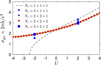
Figure 5: A counterpart of Fig. 1b of the main text showing the dependence of the anomalous Hall response of a WSM (model I) on the Hubbard $U$. We have shown the results for different cluster sizes, $N_{c}$, to illustrate that reasonable convergence has been achieved already for $N_{c}=2\times 2\times 2$.

As an example, in Fig. 5, we illustrate the convergence of the anomalous Hall response of model I with respect to the cluster size $N_{c}$ (same parameters as for Fig. 1b of the main text). It can be seen that the results for $N_{c}=2\times 2\times 2$ and $N_{c}=3\times 2\times 2$ can hardly be distinguished. Further numerical refinement due to an increased $N_{c}$ would be very costly in terms of computational resources and would not alter our results. This conclusion is reasonable given that the CPT results are well bounded by those from the mean field and strong coupling calculations, as can be seen in Fig. 1b of the main text.

Appendix C Weyl nodes of Models I and II

C.1 Model I

The tight binding part of Model I was introduced in Ref. Yang et al., 2011. Below we review the non-interacting WSM band structure, and analyze the effects of the Hubbard term on the Weyl fermions using strong and weak coupling expansions.

Non-interacting band structure: Diagonalizing the non-interacting Bloch Hamiltonian, Eq. (5) of the main text, defines the band structure

$$\xi_{n}({\bm{k}})=\pm\left[{\{2(\cos k_{x}-\cos k_{0})+m(2-\cos k_{y}-\cos k_{z})\}^{2}+4\sin^{2}k_{y}+4\sin^{2}k_{z}}\right]^{1/2}\;.$$ (25)

The hopping amplitude $t$ has been set to unity. We have also set the chemical potential to zero, as appropriate for half-filling. The non-interacting Weyl nodes are then obtained from the zeros of $\xi_{n}({\bm{k}})$:

$${\bm{k}} =(\pm k_{0},0,0)$$

$${\bm{k}} =(\pm\cos^{-1}(\cos k_{0}-m),0,\pi)\qquad \text{if}\quad|\cos k_{0}-m|\leq 1$$

$${\bm{k}} =\left(\pm\cos^{-1}(\cos k_{0}-m),\pi,0\right)\qquad \text{if}\quad|\cos k_{0}-m|\leq 1$$

$${\bm{k}} =(\pm\cos^{-1}(\cos k_{0}-2m),\pi,\pi)\qquad \text{if}\quad|\cos k_{0}-2m|\leq 1\;.$$

When $m>1$, the Hamiltonian has the minimal allowed number of Weyl nodes, i.e. only two. This is the case we focus on. The Hamiltonian of model I breaks TRS, since $\Theta H\Theta^{-1}\neq H$, where $\Theta=(-i\sigma^{y})\hat{K}$ ($\hat{K}$ is the complex conjugation operator).

As discussed in the main text, short ranged attractive or repulsive interactions in a WSM are irrelevant in the renormalization group sense. Therefore, the Weyl nodes, which are hedgehogs of the Berry curvature, cannot be destroyed by local interactions but their position in the BZ can, and generically will, change. In the following, we discuss perturbative estimates for the renormalization of the Weyl fermions induced by local interactions in both the strong and weak coupling limits.

Strong-coupling limit: Starting with the Hamiltonian of model I in the atomic limit ($t=0$)

$$H_{\rm a}=Un_{\uparrow}n_{\downarrow}-\mu(n_{\uparrow}+n_{\downarrow})+\underbrace{2(m-\cos k_{0})}_{\equiv M}c^{\dagger}\sigma_{x}c\;.$$ (27)

we perturbatively turn on the hopping to neighboring sites. Using the equations of motion technique, or alternatively the Lehmann representation, we first calculate the atomic limit Green’s functions at half-filling, $\mu=U/2$,

$$G_{\rm a,\uparrow\uparrow}(\omega)=G_{\rm a,\downarrow\downarrow}=\frac{\omega}{\omega^{2}-(M+\frac{U}{2})^{2}}\qquad G_{\rm a,\downarrow\uparrow}(\omega)=G_{\rm a,\uparrow\downarrow}=\frac{M+\frac{U}{2}}{\omega^{2}-(M+\frac{U}{2})^{2}}\;.$$ (28)

Second, we set up the topological Hamiltonian, $\mathcal{H}_{t}({\bm{k}})=-G^{-1}_{\rm a}(0)+T({\bm{k}})$, using first order perturbation theory in $t/U$. Here, $T({\bm{k}})$ is the hopping matrix, i.e. the ${\bm{k}}$-dependent part of the Bloch Hamiltonian $\mathcal{H}({\bm{k}})$. (The ${\bm{k}}$-independent part has already been included in $H_{\rm a}$.) Diagonalizing $\mathcal{H}_{t}({\bm{k}})$ gives the effective band structure (setting $t=1$)

$$\tilde{\xi}_{n}({\bm{k}})=\pm\left[{\left\{2(\cos k_{x}-\cos k_{0})+m(2-\cos k_{y}-\cos k_{z})+{U}/{2}\right\}^{2}+4\sin^{2}k_{y}+4\sin^{2}k_{z}}\right]^{1/2},$$ (29)

from which we obtain the interacting Weyl points

$${\bm{k}} =(\pm\cos^{-1}(\cos k_{0}-{U}/{4}),0,0)\qquad \text{if}\quad|\cos k_{0}-{U}/{4}|\leq 1$$

$${\bm{k}} =(\pm\cos^{-1}(\cos k_{0}-m-{U}/{4}),0,\pi)\qquad \text{if}\quad|\cos k_{0}-m-{U}/{4}|\leq 1$$

$${\bm{k}} =(\pm\cos^{-1}(\cos k_{0}-m-{U}/{4}),\pi,0)\qquad \text{if}\quad|\cos k_{0}-m-{U}/{4}|\leq 1$$

$${\bm{k}} =(\pm\cos^{-1}(\cos k_{0}-2m-{U}/{4}),\pi,\pi)\qquad \text{if}\quad|\cos k_{0}-2m-{U}/{4}|\leq 1\;.$$

The functional dependence of the Weyl points on $U$ in the strong-coupling limit is shown in Fig. 1b of the main text, in the parameter regime where only two Weyl nodes are present. Recall that in that case $\sigma_{yz}\propto 2k_{0}$, where $\pm{\bm{k}}_{0}$ are the locations of the interacting Weyl nodes.

Weak-coupling limit: The renormalization of the Weyl nodes in the weak-coupling limit $U\ll t$, can be obtained from a variational Hartree-Fock calculation. We consider the case of half-filling for which the interaction decouples as

$$Un_{r,\uparrow}n_{r,\downarrow}\to\frac{U}{2}(n_{r,\uparrow}+n_{r,\downarrow})-Um_{x}c_{r}^{\dagger}\sigma_{x}c_{r}+Um_{x}^{2}\;,$$

where we introduced the magnetization $m_{x}=\frac{1}{2}\langle c_{r}^{\dagger}\sigma_{x}c_{r}\rangle$ as an order parameter. In the weak-coupling limit we thus obtain

$$H_{\text{HF}}=\sum_{{\bm{k}}}m_{x}^{2}U+c_{{\bm{k}}}^{\dagger}\big{[}\{2t(\cos k_{x}-\cos k_{0})-Um_{x}+m(2-\cos k_{y}-\cos k_{z})\}\sigma_{x}\\ +2t\sin k_{y}\,\sigma_{y}+2t\sin k_{z}\,\sigma_{z}\big{]}c_{{\bm{k}}}\;.$$ (31)

Minimizing the ground state energy, determines the optimal variational order parameter $m_{x}$ from which we can determine the position of the renormalized Weyl nodes, see Fig. 1b of the main text.

C.2 Model II

We introduce a new model for a WSM that respects time-reversal symmetry, which thus belongs to the other family of WSMs (as opposed to model I). It is defined on the cubic lattice.

Non-interacting band structure: Model II has a charge-density-wave order determined by $H_{\rm cdw}=\epsilon\sum_{{\bm{k}}}c^{\dagger}_{{\bm{k}}}c_{{\bm{k}}+{\bm{Q}}}$, with ordering wavevector ${\bm{Q}}=(\pi,\pi,0)$. Therefore, the chemical potential in the $xy$ plane is staggered by $\pm\epsilon$. In order to solve for the non-interacting band structure of Hamiltonian, Eq. (6) of the main text, we double the unit cell and rotate it by $\pi/4$ in the $xy$ plane such that it includes 2 sites with local potentials $\epsilon$ and $-\epsilon$, respectively. The tight binding Hamiltonian thus reads

$$H_{0}=\sum_{{\bm{k}}}\begin{pmatrix}c_{{\bm{k}}}^{\dagger}&d_{{\bm{k}}}^{\dagger}\end{pmatrix}\begin{pmatrix}\epsilon+2\sigma_{z}\sin k_{z}&2\sigma_{x}\sin k_{+}+2\sigma_{y}\sin k_{-}\\ 2\sigma_{x}\sin k_{+}+2\sigma_{y}\sin k_{-}&-\epsilon+2\sigma_{z}\sin k_{z}\end{pmatrix}\begin{pmatrix}c_{{\bm{k}}}\\ d_{{\bm{k}}}\end{pmatrix}\;,$$ (32)

where $c_{{\bm{k}}}/d_{{\bm{k}}}$ is associated with the $\pm\epsilon$ sublattice. We have defined the inplane momenta $k_{\pm}=k_{X}\pm k_{Y}$, where $k_{X,Y}$ correspond to the enlarged unit cell obtained when $\epsilon\neq 0$. The associated non-interacting band structure consists of the 4 bands:

$$\xi_{n}({\bm{k}}) =\pm\left[4\sin^{2}k_{+}+4\sin^{2}k_{-}+(\epsilon+2\sin k_{z})^{2}\right]^{1/2}$$

$$\xi_{n}({\bm{k}}) =\pm\left[4\sin^{2}k_{+}+4\sin^{2}k_{-}+(\epsilon-2\sin k_{z})^{2}\right]^{1/2}\;.$$

This band structure defines a WSM with 16 Weyl nodes located at a combination of any

$$k_{X} \in\{0,\pi\}\;,\qquad k_{Y}\in\{0,\pi\}\;,\qquad k_{z}\in\{\pm\sin^{-1}\epsilon/2,\pi\pm\sin^{-1}\epsilon/2\}\;.$$

The Hamiltonian of model II preserves TRS, $\Theta H\Theta^{-1}=H$. However, inversion symmetry $PH({\bm{k}})P^{-1}=H(-{\bm{k}})$ is explicitly broken.

Appendix D Lifetime of Weyl and Dirac excitations

We provide a brief analysis of the lifetime of the nodal excitations in Weyl and Dirac liquids in $d$ spatial dimensions. We also discuss the marginal liquid case that arises with long-range Coulomb repulsion. First, the Dirac/Weyl liquid states are obtained by considering linearly dispersing nodal fermions interacting with short-ranged interactions. For $d\geq 2$, such interactions, both repulsive and attractive, are irrelevant in the renormalization group sense. Indeed, a coupling $U$ parameterizing a four-fermion contact term (say of density-density type $\rho(x)^{2}$) scales like $[U]=\omega^{d-1}$, where $\omega$ is the real frequency (or energy). Thus when $d>1$, $U$ vanishes as $\omega^{d-1}$ at low energy $\omega\rightarrow 0$. Therefore, the $U$-driven scattering rate of the Weyl or Dirac excitations in the liquid can be obtained from a perturbative scaling analysis of the self-energy:

$$\gamma(\omega) \equiv\operatorname{Im}\Sigma_{R}(\omega+i0^{+},{\bm{k}}_{0})\,,$$ (33)

$$=\omega(U_{\rm eff}/\Lambda)^{2}\;\sim\;|\omega|^{2d-1}\,,$$ (34)

where ${\bm{k}}_{0}$ corresponds to the nodal point, and $\Lambda$ is a UV energy scale such as the bandwidth. The overall factor of $\omega$ in the second equality arises on dimensional grounds, while $U_{\rm eff}$ is the effective running coupling constant describing the short-range interaction. It appears squared due to the perturbative interaction where a fermion creates a single virtual particle-hole pair. From the discussion above, we have $U_{\rm eff}(\omega)\sim|\omega|^{d-1}$, yielding the energy-dependent scattering rate $\omega^{2d-1}$. This confirms that for $d>1$, the excitations become sharp as $\omega\rightarrow 0$. In other words, an infinitely lived quasiparticle emerges at the node. In the case of Weyl or Dirac liquids in $d=3$, we obtain $\gamma(\omega)\sim|\omega|^{5}$. For $d=2$, we recover the standard result for two-dimensional Dirac liquids, such as graphene with short-range interactions: $\gamma\sim\omega^{3}$.

In the presence of the $1/r$ Coulomb repulsion, the Weyl/Dirac liquid breaks down marginally. Indeed, in both two and three dimensions the coupling parameterizing the Coulomb $1/r$ interaction in the action, $V\int dtd^{d}{\bm{x}}d^{d}{\bm{y}}\rho(x)\rho(y)/|{\bm{x}}-{\bm{y}}|$, is marginal. In other words, $V_{\rm eff}\sim\omega^{0}$, so that the scattering rate becomes $\gamma\sim\omega V_{\rm eff}^{2}\sim\omega$, implying a marginal destruction of the nodal quasiparticle in both $d=2$Das Sarma et al. (2007) and $3$Abrikosov and Beneslavskii (1971).

References

- Geim and Novoselov (2007) A. K. Geim and K. S. Novoselov, Nat Mater 6, 183 (2007).
- Castro Neto et al. (2009) A. H. Castro Neto, F. Guinea, N. M. R. Peres, K. S. Novoselov, and A. K. Geim, Rev. Mod. Phys. 81, 109 (2009).
- Hasan and Kane (2010) M. Z. Hasan and C. L. Kane, Rev. Mod. Phys. 82, 3045 (2010).
- Qi and Zhang (2011) X.-L. Qi and S.-C. Zhang, Reviews of Modern Physics 83, 1057 (2011).
- Wan et al. (2011) X. Wan, A. M. Turner, A. Vishwanath, and S. Y. Savrasov, Phys. Rev. B 83, 205101 (2011).
- Xu et al. (2011) G. Xu, H. Weng, Z. Wang, X. Dai, and Z. Fang, Phys. Rev. Lett. 107, 186806 (2011).
- Witczak-Krempa and Kim (2012) W. Witczak-Krempa and Y. B. Kim, Phys. Rev. B 85, 045124 (2012).
- Witczak-Krempa et al. (2014) W. Witczak-Krempa, G. Chen, Y. B. Kim, and L. Balents, Annual Review of Condensed Matter Physics 5, 57 (2014).
- Burkov and Balents (2011) A. A. Burkov and L. Balents, Phys. Rev. Lett. 107, 127205 (2011).
- Nielsen and Ninomiya (1983) H. B. Nielsen and M. Ninomiya, Physics Letters B 130, 389 (1983).
- Haldane (2004) F. D. Haldane, Phys. Rev. Lett. 93, 206602 (2004).
- Yang et al. (2011) K.-Y. Yang, Y.-M. Lu, and Y. Ran, Phys. Rev. B 84, 075129 (2011).
- Turner and Vishwanath (2013) A. M. Turner and A. Vishwanath, ArXiv e-prints (2013), arXiv:1301.0330 [cond-mat.str-el] .
- Vafek and Vishwanath (2014) O. Vafek and A. Vishwanath, Annual Review of Condensed Matter Physics 5, 83 (2014).
- Parameswaran et al. (2014) S. A. Parameswaran, T. Grover, D. A. Abanin, D. A. Pesin, and A. Vishwanath, Phys. Rev. X 4, 031035 (2014).
- Hosur (2012) P. Hosur, Phys. Rev. B 86, 195102 (2012).
- Potter et al. (2014) A. C. Potter, I. Kimchi, and A. Vishwanath, ArXiv e-prints (2014), arXiv:1402.6342 [cond-mat.mes-hall] .
- Panfilov et al. (2014) I. Panfilov, A. A. Burkov, and D. A. Pesin, Phys. Rev. B 89, 245103 (2014).
- Volovik (2003) G. A. Volovik, The Universe in a Helium Droplet (Oxford University Press, 2003).
- Go et al. (2012) A. Go, W. Witczak-Krempa, G. S. Jeon, K. Park, and Y. B. Kim, Physical Review Letters 109, 066401 (2012).
- Wang and Zhang (2012a) Z. Wang and S.-C. Zhang, Phys. Rev. B 86, 165116 (2012a).
- Mastropietro (2013) V. Mastropietro, ArXiv e-prints (2013), arXiv:1310.5638 [cond-mat.str-el] .
- Sekine and Nomura (2013) A. Sekine and K. Nomura, ArXiv e-prints (2013), arXiv:1309.1079 [cond-mat.str-el] .
- Note (1) This notation was introduced in Ref.\tmspace+.1667em\rev@citealpnumwang_Ht in the context of interacting topological insulators. We keep it, although we deal with gapless systems. This is motivated because the topological Hamiltonian captures the Berry phase properties of the electrons (such as hedgehogs).
- Sénéchal et al. (2000) D. Sénéchal, D. Perez, and M. Pioro-Ladrière, Phys. Rev. Lett. 84, 522 (2000).
- Abrikosov and Beneslavskii (1971) A. A. Abrikosov and S. D. Beneslavskii, JETP 32, 699 (1971).
- Nandkishore et al. (2012) R. Nandkishore, M. A. Metlitski, and T. Senthil, Phys. Rev. B 86, 045128 (2012).
- Wang et al. (2012) Z. Wang, X.-L. Qi, and S.-C. Zhang, Phys. Rev. B 85, 165126 (2012).
- Wang and Zhang (2012b) Z. Wang and S.-C. Zhang, Phys. Rev. X 2, 031008 (2012b).
- Hung et al. (2013) H.-H. Hung, L. Wang, Z.-C. Gu, and G. A. Fiete, Phys. Rev. B 87, 121113 (2013).
- Lang et al. (2013) T. C. Lang, A. M. Essin, V. Gurarie, and S. Wessel, Phys. Rev. B 87, 205101 (2013).
- Deng et al. (2013) X. Deng, K. Haule, and G. Kotliar, Phys. Rev. Lett. 111, 176404 (2013).
- Laubach et al. (2013) M. Laubach, J. Reuther, R. Thomale, and S. Rachel, ArXiv e-prints (2013), arXiv:1312.2934 [cond-mat.str-el] .
- Grandi et al. (2014) F. Grandi, F. Manghi, O. Corradini, C. M. Bertoni, and A. Bonini, ArXiv e-prints (2014), arXiv:1404.1287 [cond-mat.str-el] .
- Fang et al. (2012) C. Fang, M. J. Gilbert, X. Dai, and B. A. Bernevig, Phys. Rev. Lett. 108, 266802 (2012).
- So (1985) H. So, Progress of Theoretical Physics 74, 585 (1985).
- Ishikawa and Matsuyama (1986) K. Ishikawa and T. Matsuyama, Z. Phys. C 33, 41 (1986).
- Maciejko and Nandkishore (2013) J. Maciejko and R. Nandkishore, ArXiv e-prints (2013), arXiv:1311.7133 [cond-mat.str-el] .
- Hosur and Qi (2013) P. Hosur and X. Qi, Comptes Rendus Physique 14, 857 (2013), arXiv:1309.4464 [cond-mat.str-el] .
- Lundgren et al. (2014) R. Lundgren, P. Laurell, and G. A. Fiete, ArXiv e-prints (2014), arXiv:1407.1435 [cond-mat.str-el] .
- Maciejko et al. (2014) J. Maciejko, V. Chua, and G. A. Fiete, Phys. Rev. Lett. 112, 016404 (2014).
- Engelsberg and Schrieffer (1963) S. Engelsberg and J. R. Schrieffer, Phys. Rev. 131, 993 (1963).
- Mahan (2000) G. Mahan, Many-Particle Physics, Physics of Solids and Liquids (Springer, 2000).
- Das Sarma et al. (2007) S. Das Sarma, E. H. Hwang, and W.-K. Tse, Phys. Rev. B 75, 121406 (2007).
- Wang and Yan (2013) Z. Wang and B. Yan, Journal of Physics: Condensed Matter 25, 155601 (2013).