Geodesic Study of Regular Hayward Black Hole

Abstract

This paper is devoted to study the geodesic structure of regular Hayward black hole. The timelike and null geodesic have been studied explicitly for radial and non-radial motion. For timelike and null geodesic in radial motion there exists analytical solution, while for non-radial motion the effective potential has been plotted, which investigates the position and turning points of the particle. It has been found that massive particle moving along timelike geodesics path are dragged towards the BH and continues move around BH in particular orbits.

Key Words: Hayward Black Holes; Regular Black Holes; Geodesics.
 PACS: 04.70.Bw, 04.70.Dy, 95.35.+d

1 Introduction

Since yet, we do not have perfectly reliable candidate to test the phenomenological aspects of quantum theory of gravity. Spacetime singularity is one of the avoidable issue in quantum theory of gravity, so research on properties of regular black hole solutions is much important in quantum theory of gravity. The regular black hole solutions have event horizons but there is the absence of such region where closed timelike curves may exist, i.e., such solutions are singularity free. Of course, these are non-vacuum solutions of Einstein field equations and source of gravity is taken as some form of exotic field, non-linear electrodynamics or some modified form of gravity.

The regular BH solution was formulated by Bardeen which is commonly known as Bardeen BH (Bardeen 1968, Borde 1994 and Borde 1997). Later on, Ayon-Beato and Garcia (Ayon-Beato and Garcia 1998) carried out the coupling of Einstein field equation and Maxwell field equations and derived the charged version of Bardeen. For this version of regular BH, they take the non-linear electric field as a source of charge for the solution of Maxwell field equations. The physical nature of charged regular BH was studied by the Bronikov (Bronnikov, 2000, Bronnikov, 2001), he showed analytically that charged regular BHs are not correct solutions of the field equations. The main cause of such unsatisfactory interpretation was the addition of electromagnetic Lagrangian quite differently in the various direction of the space under consideration. On the other hand a correct solution of the field equations was given by Hayward (Hayward, 2006), which is free of charge term and its physical aspects are quite similar to Bardeen BH. The limits of the Hayward BH are quite correct as in the limit $r\rightarrow\infty$, it corresponds to Schwarzschild BH and for $r\rightarrow 0$, it corresponds to de-Sitter BH. The particular choice of solution parameters imply that it may have two horizons, single horizon and no horizon. A lot of work (Sharif and Abbas 2013a, 3013b, 2013c) has been done on the nature and structure of regular BH.

One of the most challenging tasks in theoretical physics is to combine quantum theory and general relativity, which can be done by clarifying the structure of singularities occurring in general theory of relativity. In this regard the geodesic study near the gravitational field of compact objects is much important. This study was initiated by Chandrasekhar (Chandrasekhar 1983), he studied the geodesic of Schwardzschild, Reissner-Nordstr$\ddot{o}$m and Kerr BHs. Since then there has been growing interest to study the geodesic around BHs. Many researches have studied the geodesics of various BH like geodesic study of the schwarzschild BH in Rainbow gravity was studied by Leiva et al.(2009). Guha and Bhattacharya (2012) the geodesic motion around five dimensional charged anti-de Sitter BH. Fernando et al.(2003) have studied the null geodesic of Schwarzschild BH in the presence of quintessence.

Recently, Kalam et al.(2014) have explored the geodesic of charged BH in non-linear electrodynamics. Curz et al.(2013) have studied the geodesic structure of topological Lifshitz black hole in 1+2 dimension. Mosaffa (2011) have explored the geodesic structure in Horava-Lifshitz BH. Setare and Mansouri (2003) have investigated the null geodesics in Horava-Lifshitz gravity. Several authors have discussed the geodesics of BHs with cosmological constant. In this paper, we have studied the geodesic of a regular Hayward BH, which has properties of Schwarzschild as well as de-Sitter BH.

2 Geodesics of Regular Hayward Black Hole

The static spherically symmetric space-time is described by the Hayward metric (Hayward 2006) which is given by

$${ds}^{2}=-f(r)dt^{2}+\frac{1}{f(r)}dr^{2}+r^{2}(d\theta^{2}+\sin^{2}{\theta}d\phi^{2}),$$ (1)

where $f(r)=1-\frac{2mr^{2}}{r^{3}+2l^{2}m}$ with $m$ corresponding to mass of the black hole and $l$ is a convenient encoding of the central energy density $3/8\pi l^{2}$, assumed positive. The lapse function $f(r)$ for $\lim r\rightarrow\infty$ reduces to $1-\frac{2m}{r}+O(\frac{1}{r^{4}})$, while at $\lim r\rightarrow 0$ it reduces to $1-\frac{r^{2}}{l^{2}}+O(r^{4})$. From the asymptotic behavior of the metric function, it is clear that Hayward BH becomes Schwarzschild BH at large value of $r$ and for small value of $r$, it is de-Sitter BH. The Hayward BH solution is non-singular (regular) as all the scalars curvature are finite and regular at center of the metric where $r\rightarrow 0$ , which can be verified by scalars of this metric

$$R = \frac{24l^{2}m^{2}(r^{3}-4l^{2}m)}{(r^{3}+2l^{2}m)^{3}},\quad{\lim}_{r\rightarrow 0}R=-\frac{12}{l^{2}},$$ (2)

$$\ R_{\mu\nu}R^{\mu\nu} = \frac{288m^{4}l^{4}(5r^{6}-6r^{3}l^{2}m+8l^{4}m^{2})}{(r^{3}+2ml^{2})^{6}},\quad{\lim}_{r\rightarrow 0}R_{\mu\nu}R^{\mu\nu}=\frac{36}{l^{4}},$$ (3)

$$R_{\mu\nu\lambda\eta}R^{\mu\nu\lambda\eta} = \frac{48m^{2}}{(r^{3}+2ml^{2})^{6}}\left(r^{12}-8r^{9}ml^{2}+72m^{2}r^{6}l^{4}-16r^{3}m^{3}l^{4}+32m^{4}l^{8}\right)$$

$$\ {\lim}_{r\rightarrow 0}R_{\mu\nu\lambda\eta}R^{\mu\nu\lambda\eta} = \frac{24}{l^{4}}.$$ (4)

This metric function $f(r)$ reduces to the Schwarzschild BH for $l=0$ and is flat for $m=0$. By the analysis of $f(r)$ for zeros, we see that a critical mass $m_{*}=(3\sqrt{3}/4)l$ and $r_{*}=\sqrt{3}l$ such that $r>0$, $f(r)$ has no zero if $m<m_{*}$ and if $m=m_{*}$ there is one zero at $r=r_{*}$ and if $m>m_{*}$ there are two zeros at $r=r_{\pm}$, the event and inner horizons. This is shown in figure 1.

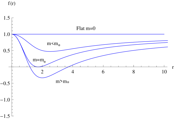
Figure 1: Behavior of $f(r)$ for fixed value of parameter $l$ and different values of $m$

.

Now, the Lagrangian for metric (1) is

$${\mathcal{L}}=-\frac{1}{2}\left(-f(r)\dot{t}^{2}+\frac{1}{f(r)}\dot{r}^{2}+r^{2}\dot{\theta}^{2}+r^{2}\sin^{2}{\theta}\dot{\phi}^{2}\right),$$ (5)

where dot indicates the differentiation with respect to affine parameter $\tau$.

The Euler-Lagrange equation is

$$\frac{d}{d\tau}\left(\frac{\partial{\mathcal{L}}}{\partial\dot{x}^{\mu}}\right)-\frac{\partial{\mathcal{L}}}{\partial x^{\mu}}=0,$$ (6)

using Eq.(5) in Eq.(6), we get

$$\dot{t}=\frac{E}{f(r)},$$ (7)

$$r^{2}\sin^{2}{\theta}\dot{\phi}=J,$$ (8)

where $E$ and $J$ are constant of motion which correspond to the Killing vectors $\partial_{t}$ and $\partial_{\phi}$, respectively. Further, we take $\theta=\frac{\pi}{2}$ and $\dot{\theta}=0$ as initial conditions. Hence Eqs.(7) and (8) yield

$$\dot{t}=\frac{E}{f(r)},$$ (9)

$$r^{2}\dot{\phi}=J.$$ (10)

Using Eqs.(9) and (10) in Eq.(5),

$$\frac{1}{f(r)}\left(\frac{dr}{d\tau}\right)^{2}=\frac{E^{2}}{f(r)}-\frac{J^{2}}{r^{2}}-L,$$ (11)

where $L=2{\mathcal{L}}$ and $L$ has values 0 and 1. Equation (11) becomes for radial motion

$$\frac{1}{f(r)}\left(\frac{dr}{d\tau}\right)^{2}=\frac{E^{2}}{f(r)}-L.$$ (12)

Here,

$$\frac{dr}{dt}=\frac{d\tau}{dt}\frac{dr}{d\tau}$$ (13)

$$\left(\frac{dr}{dt}\right)^{2}=\left.f^{2}(r)\left[1-\frac{L}{E^{2}}f(r)\right]\right..$$ (14)

This is the master equation for the radial geodesic motion. In following, we shall apply this equation explicitly for photon-like particles $L=0$ and massive particles $L=1$.

2.1 Photon-like Particle Motion ($L$=0)

Equation (14) gives

$$\left(\frac{dr}{dt}\right)^{2}={f(r)}^{2},$$ (15)

after putting the value of $f(r)$, we get

$$\pm t=\int\frac{dr}{{1-\frac{2mr^{2}}{r^{3}+2l^{2}m}}}.$$ (16)

Integration of above equation leads to

$$\pm t = \frac{1}{9}\left[\frac{(42)^{2/3}m^{5/3}\log(2l^{2/3}\sqrt[3]{m}+2^{2/3}r)}{l^{2/3}}-\frac{(42)^{2/3}\sqrt{3}m^{5/3}\tan^{-1}\left(\frac{\frac{2^{2/3}r}{l^{2/3}\sqrt[3]{m}}-1}{\sqrt{3}}\right)}{l^{2/3}}\right.$$

$$+ \left.9r+\frac{12m^{2}r^{2}}{2l^{2}m+r^{3}}+6m\log{(2l^{2}m+r^{3})}\right.$$

$$- \left.{\frac{(22)^{2/3}m^{5/3}\log{\left(2l^{4/3}m^{2/3}-2^{2/3}l^{2/3}\sqrt[3]{m}r+\sqrt[3]{2}r^{2}\right)}}{l^{2/3}}}\right].$$

The relation between the time and distance is shown in left graph of figure 2.

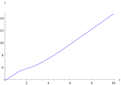
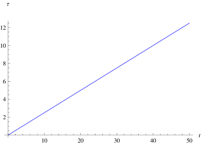
Figure 2: The left graph shows the behavior of $r$ and $t$ from Eq.(2.1) (when $m$=2 and $l$=1). The right graph shows the relation of Eq.(19) with $E=4$.

Now, from Eq.(14), when $L=0$, the relation between $\tau$ and $r$ is given by

$$\left(\frac{dr}{d\tau}\right)^{2}=E^{2},$$ (18)

the above equation implies that

$$\pm E\tau=r.$$ (19)

The changing of proper time $(\tau)$ and $r$ is shown in right graph of figure 2.

2.2 Massive particle motion ($L$=1)

Here we deal with the motion of massive particles when the trajectories of the particles are radial direction of BH. From Eq.(14), we get

$$\left(\frac{dr}{dt}\right)^{2}=\left[f^{2}(r)-\frac{f^{3}(r)}{E^{2}}\right].$$ (20)

Integration of this equation yields

$$\pm t = \frac{1}{18}\left[\frac{(42)^{2/3}m^{5/3}\log{(2l^{2/3}\sqrt[3]{m}+2^{2/3}r)}}{E^{2}l^{2/3}}-\frac{(42)^{2/3}\sqrt{3}m^{5/3}\tan^{-1}\left({\frac{2^{2/3}r}{l^{2/3}\sqrt[3]{m}}}-1\right)}{E^{2}l^{2/3}}\right.$$ (21)

$$+ \left.\frac{12m^{2}r^{2}}{E^{2}(2l^{2}m+r^{3})}-\frac{(22)^{2/3}m^{5/3}\log{(2l^{4/3}m^{2/3}-2^{2/3}l^{2/3}\sqrt[3]{m}r+\sqrt[3]{2}r^{2})}}{E^{2}l^{2/3}}+9r(E^{2}+2)\right.$$

$$+ \left.\frac{6(E^{4}+2E^{2}-1)m\log{(2l^{2}+r^{3})}}{E^{2}}\right].$$

The relation between $t$ and $r$ for the massive particles is shown in the left graph of figure 3.

From Eq. (12), we get

$$\left(\frac{dr}{d\tau}\right)^{2}=E^{2}-f(r).$$ (22)

This implies that

$$\pm\tau=\int\frac{dr}{\sqrt{E^{2}-1+\frac{2mr^{2}}{r^{3}+2ml^{2}}}}.$$ (23)

After integrating, we get

$$\pm\tau=\frac{r}{2}+E^{2}r-\frac{1}{3}\log{(2l^{2}m+r^{3})}.$$ (24)

This is the relation between proper time $(\tau)$ and $(r)$, which is shown in right graph of figure 3.

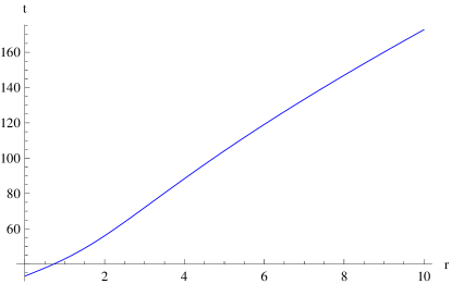
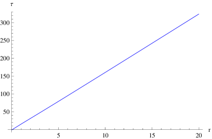
Figure 3: The left graph show the behave of $r$ and $t$ from Eq.(21) (when $m$=2, $E=4$ and $l$=1). The right graph show the relation of Eq. (24) with ($m=2$, $l=1$ and $E=4$)

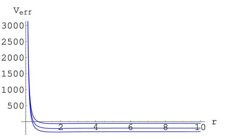
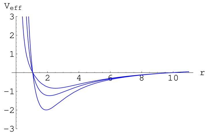
Figure 4: This is shape of effective potential $(V_{eff})$ for circular motion in Hayward geometry. The graph has been plotted for $m=3$, $E=100,200,300,J=10$ and $l=1$.

Figure 5: This is shape of effective potential $(V_{eff})$ for circular motion in Hayward geometry. The graph has been plotted for $m=3,E=0,J=10,20,30$ and $l=1.$

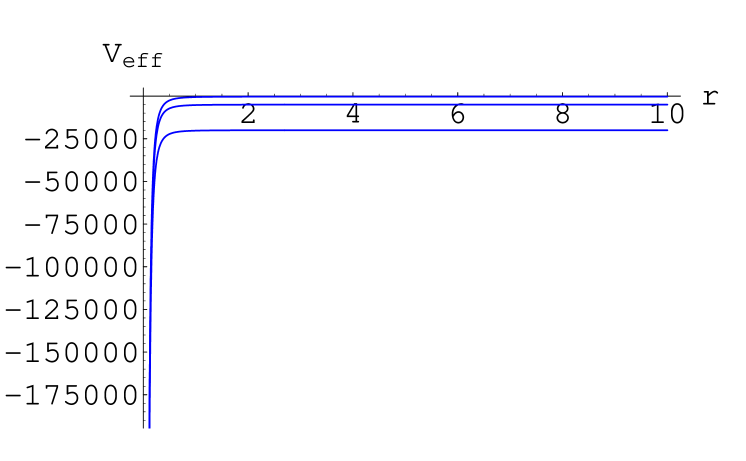
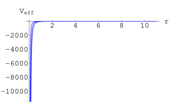
Figure 6: This is the shape of effective potential $(V_{eff})$ for circular motion in Schwarzschild geometry ($l=0$ in Eq.(26)). The graph has been plotted for $m=3$, $E=100,200,300$ and $J=10$.

Figure 7: This is the shape of effective potential $(V_{eff})$ for circular motion in Schwarzschild geometry ($l=0$ in Eq.(26)). The graph has been plotted for $m=3$, $E=0$ and $J=10,20,30$.

3 Effective Potential

From the geodesic Eq.(11)

$${\dot{r}}^{2}\equiv\left(\frac{dr}{d\tau}\right)^{2}=E^{2}-f(r)\left(\frac{J^{2}}{r^{2}}+L\right).$$ (25)

Comparing above equation with equation of motion $\frac{\dot{r}^{2}}{2}+V_{eff}=0$, we get

$$V_{eff}=-\frac{1}{2}\left[E^{2}-f(r)\left(\frac{J^{2}}{r^{2}}+L\right)\right].$$ (26)

This leads to Schwarzschild BH effective potential when $l=0$ in lapse function $f(r)$ of the Hayward BH.

3.1 For Photon-like Particle ($L$=0)

Consider the radial geodesic when $J=0$. Then, $V_{eff}$ is given by

$$V_{eff}=-\frac{1}{2}E^{2}.$$ (27)

This show that particle will behave like a free particle i.e., its $V_{eff}=0$, for $E=0$ .

For circular geodesic case, $J\neq 0$, the effective potential can be written as,

$$V_{eff}=-\frac{E^{2}}{2}+\frac{J^{2}}{2r^{2}}\left(1-\frac{2mr^{2}}{r^{3}+2l^{2}m}\right).$$ (28)

In the limit $r\rightarrow 0$, $V_{eff}$ attains a large value and when $r\rightarrow\infty$, ${V_{e}ff}\rightarrow-\frac{E^{2}}{2}$, and graph shown in figures 4 and 5. By definition horizon would occur at such values of radial position $r$ where $f(r)=0$, so from Eq.(26), we have $V_{eff}=-\frac{1}{2}E^{2}<0$, for every $E$. In this case particles have real velocity between the horizons.

3.2 For Massive Particle ($L$=1)

In this case effective potential is

$$V_{eff}=-\frac{1}{2}\left[E^{2}-f(r)\left(\frac{J^{2}}{r^{2}}+1\right)\right].$$ (29)

For $J=0$, we get same value of $V_{eff}$ as in case of photon-like particle. It is interesting to study the motion of massive particle for $E\geq 0$. When $E=0$ and $J=0$, we get

$$V_{eff}=\frac{1}{2}\left[1-\frac{2mr^{2}}{r^{3}+2l^{2}m}\right].$$ (30)

This equation is nothing but the effective potential in term of lapse function. The roots of $V_{eff}$ will be same as the roots of $f(r)$ in figure1. Depending upon the values of the parameters particles can move inside the BH. For $E\neq 0$ and $J=0$, we have $V_{eff}=-\frac{E^{2}}{2}+f(r)$. This has same interpretation as in case of motion of photon at the horizon, i.e., $f(r)=0$ at horizon and $V_{eff}<0$, particles have real velocity between the horizons. In the limit $r\rightarrow\infty$, this potential attains a constant value $V_{eff}\rightarrow\frac{1-E^{2}}{2}$.

Now, we consider the non-vanishing angular momentum case $J\neq 0$, with $E=0$, the effective potential becomes

$$V_{eff}=\frac{1}{2}\left(1-\frac{2mr^{2}}{r^{3}+2l^{2}m}\right)\left(\frac{J^{2}}{r^{2}}+1\right).$$ (31)

In this case the shape of potential coincides with the roots the lapse functions which implies that particles tracing out the timlike trajectories are captured by the BH, which makes these particles to move in the circular orbits of fixed radius. The existence of minima in figures 4 and 5 indicate the stability of circular orbit.

4 Conclusion

In this paper, we have investigated the structure of timelike and null geodesics of Hayward regular BH. The radial and non-radial geodesics motion for both massless (photon) and massive particles have been analyzed in explicitly. In case of radial motion, we have determined the analytic solution of equation of motion, which exhibit the relation between radial distance and time/proper time. During the radial motion, the photon as well as massive particles undergoes a small deviation in distance-time relation, while distance-proper time relationships are linear as shown in figure 2 and 3. These relations are independent of parameters of he BH and only depends on nature of geodesics (radial or non-radial). The effective potential for radial motion of photon-like particles in figures 4 and 5 imply that these can behave as free particle if its energy is zero.

For the non-radial motion $J\neq 0$, we have plotted the effective potential for particular choice of parameters. When $J\neq 0$, the massless particles have real velocity and these are bounded to move inside the horizons of the BH. For massive particle moving along circular geodesic, when $E=0$, $J\neq 0$, the effective potential has same graph as the metric function plotted for the horizon in figure 1. Hence particle moving along timelike curved path are attracted by the gravity of BH in such a way that particles continues to circulate around BH in particular orbits. The minima in the effective potential of non-radial motion of massive particles in implies that the circular orbits are stable.

The general relativity was experimentally tested in a weak gravitational field. Testing general relativity in strong gravitational field requires the investigation of some astrophysical phenomena near compact objects, such as BH or a neutron star. Astrophysical observations of galaxies imply that their centres are occupied by the massive dark objects. The arguments suggest that these are supermassive black holes. The observational targets to test the Einstein theory of relativity in a strong gravitational field is gravitational lensing. The basic tool for studying the gravitational lensing near a massive object is the geodesic study of that object. The gravitational lensing through Schwarzschild BH in the weak gravity region ( i.e.; for small deflection angle) is well-known. Kling et al. (2000) have adopted the numerical approach for gravitational lensing theory based on the approximate solutions of the geodesics equations. Virbhadra and Ellis (2000) have introduced a lens equation that allows for the large bending of light near a black hole, they model the Galactic supermassive Schwarzschild lens and study point source lensing in the strong gravitational field region. The geodesic study presented in this paper will be helpful for studying the gravitational lensing of Hayward BH. This will be done explicitly in an other investigation.

Acknowledgment

We highly appreciate the fruitful comments of the anonymous referee for the improvements of the paper.

References

- [1] Ayon-Beato, A., and Garcia, A.: Phys. Rev. Lett.80,(1998)5056
- [2] Bardeen,J.: Proceedings of GR5, Tiis, U.S.S.R. (1968)
- [3] Bronnikov, K.: Phys. Rev. Lett. 85,(2000)4641
- [4] Bronnikov, K.: Phys. Rev. D63,(2001)044005
- [5] Borde, A.: Phys. Rev. D50,(1994)3392
- [6] Borde, A.: Phys. Rev. D55,(1997)7615
- [7] Chandrasekhar, S. The Mathematical theory of black hole.(Oxford University Press, 1983)
- [8] Cruz, N., Olivares, M. and Villaueva, J.R.: Eur. Phys.C73,(2013)2485
- [9] Fernanado, S., Krug, D. and Curry, C.: Gen. Relativ.Gravit. 35,(2003)1243
- [10] Guha, S. and Bhattacharya, P.: J. Phys. Conf. Series 405,(2012)012017
- [11] Hayward, S.A.: Phys. Rev. Lett. 96,(2006)031103
- [12] Kling, T.P., Newman, E.T., Perez, A. Phys. Rev. D61, (2000)104007
- [13] Kalam, M., Farhad, N. and Hossein, S.K.: Int. J. Theor.Phys. 53,(2014)339
- [14] Leiva, C., Saavedra, J. and Villanueva, J.: Mod. Phys. Lett . A4,(2009)1443
- [15] Mosaffa, A.E.: Phys. Rev. D83,(2011)124006
- [16] Setare, M.R. and Mansouri, R.: Int. J. Mod. Phys.A18,(2003)4443
- [17] Sharif, M., Abbas, G.: J. Phys. Soc. Jpn. 82, (2013a)034006
- [18] Sharif, M., Abbas, G.: Chinese Phys. B22, (2013b)030401
- [19] Sharif, M., Abbas, G.: Eur. Phys. J. Plus 28, (2013c)10
- [20] Virbhadra, K.S., Ellis, G.F.R.: Phys. Rev. D62, (2000)084003
- [21]