The lattice gradient flow at tree-level and its improvement

Abstract

The Yang-Mills gradient flow and the observable $\langle E(t)\rangle$, defined by the square of the field strength tensor at $t>0$, are calculated at finite lattice spacing and tree-level in the gauge coupling. Improvement of the flow, the gauge action and the observable are all considered. The results are relevant for two purposes. First, the discretization of the flow, gauge action and observable can be chosen in such a way that $O(a^{2})$, $O(a^{4})$ or even $O(a^{6})$ improvement is achieved. Second, simulation results using arbitrary discretizations can be tree-level improved by the perturbatively calculated correction factor normalized to one in the continuum limit.

1 Introduction and summary

The lattice version of the Yang-Mills gradient flow Luscher:2009eq ; Luscher:2010iy ; Luscher:2010we ; Luscher:2011bx has been proven to be extremely useful in simulations of lattice gauge theories. Applications include scale setting Borsanyi:2012zs ; Bazavov:2013gca ; Sommer:2014mea , measuring the renormalized gauge coupling Fodor:2012td ; Fodor:2012qh ; Fritzsch:2013je ; Fritzsch:2013hda ; Ramos:2013gda ; Fritzsch:2013yxa ; Rantaharju:2013bva ; Luscher:2014kea and thermodynamics Asakawa:2013laa , while some of the important theoretical developments include chiral perturbation theory aspects Bar:2013ora , its relation to the energy momentum tensor Suzuki:2013gza ; DelDebbio:2013zaa ; Makino:2014taa and chiral symmetry Luscher:2013cpa ; Shindler:2013bia .

In all of these applications the size of cut-off effects is an important question and so far has not been systematically explored, although see Cheng:2014jba for some work in this direction. The observable most commonly used is $E(t)$, the expectation value of the field strength squared at $t>0$. Its discretization is affected by three building blocks of the calculation: (1) a choice needs to be made for the gauge action used along the gradient flow, (2) one needs to choose a discretized dynamical gauge action used for generating the configurations, and finally (3) one needs to choose a discretization for the observable $E$. Notice that in the continuum all three choices define the same $F_{\mu\nu}F_{\mu\nu}$ corresponding to three (potentially different) discretizations of $F_{\mu\nu}F_{\mu\nu}$.

In this work a broad family of discretizations is considered. Each of the three building blocks is chosen to be the Symanzik improved gauge action with three different improvement coefficients, $c_{1f}$ for the flow, $c_{1g}$ for the dynamical action and $c_{1e}$ for the observable. For the observable $E$ we will also consider the symmetric clover-type discretization which does not depend on any parameters.

The goal of the present work is twofold. First, we would like to calculate the optimal values for the parameters $c_{1f}$, $c_{1g}$ and $c_{1e}$ in order to achieve as high an order of improvement as possible. We will see that it is possible to choose these 3 parameters such that $O(a^{6})$ improvement is achieved. If the clover observable is used $c_{1f}$ and $c_{1g}$ can be chosen to achieve $O(a^{4})$ improvement. If the dynamical gauge action is considered fixed, i.e. $c_{1g}$ is considered fixed, $c_{1f}$ and $c_{1e}$ can be chosen to arrive at $O(a^{4})$ improvement, or if the clover observable is used then $c_{1f}$ may be chosen to achieve $O(a^{2})$ improvement.

Second, if simulations and measurements are performed with any set of parameters the resulting $\langle t^{2}E(t)\rangle$ expectation value may be tree-level improved by the perturbatively calculated correction factor normalized to one in the continuum limit. The improved data will lead to the same continuum limit as the unimproved one but the size of cut-off effects will be smaller. We will discuss the calculation of the correction factor both in finite and infinite volume.

Since our discussion is at tree-level, fermions play no role. In the following the index $1$ will be dropped from the $c_{1}$ improvement coefficients and hence they will be labelled as $c_{f},c_{g},c_{e}$.

The organization of the paper is as follows. In section 2 the gradient flow is reviewed briefly, in section 3 the lattice perturbation theory setup at tree-level is outlined and the results are given up to $O(a^{8})$. Various improved flow setups are explained in section 4 whereas the application of our formulae for scale setting in QCD is given in section 5. Finite volume effects are discussed in section 6 which are important for running coupling applications. The usefulness of tree-level improvement is demonstrated numerically in section 7 using previously published data. Finally in section 8 we close with a conclusion and outline several directions to pursue in the future along the lines presented in this paper.

2 Gradient flow

The gradient flow Luscher:2009eq ; Luscher:2010iy ; Luscher:2010we evolves the gauge field $A_{\mu}$ in an auxiliary variable $t$ by

$$\frac{dA_{\mu}(t)}{dt}=-\frac{\delta S_{\rm YM}}{\delta A_{\mu}}\;,$$ (1)

where $S_{\rm YM}$ is the pure Yang-Mills action. Clearly $t$ is of mass dimension $-2$. Once an observable is given, ${\cal O}(A_{\mu})$, the idea of the gradient flow framework is that in the path integral one integrates over the initial condition $A_{\mu}(0)$ while the observable is evaluated at $t>0$, $\langle{\cal O}(A_{\mu}(t))\rangle$. Under certain circumstances originally $UV$-divergent composite operators become finite for $t>0$ and one may think of the flow as a renormalization prescription.

In most applications the observable is $E=-\frac{1}{2}{\rm Tr}F_{\mu\nu}F_{\mu\nu}$. The resulting finite $t$-dependent quantity can be expanded in renormalized perturbation theory as Luscher:2010iy

$$\langle t^{2}E(t)\rangle=\frac{3(N^{2}-1)g^{2}}{128\pi^{2}}\left(1+O(g^{2})\right)\;,$$ (2)

where $g$ is a suitably defined renormalized coupling, for instance in $\overline{\rm MS\kern-0.5pt}\kern 0.5pt$. The corresponding bare perturbative series is similar with $g$ replaced by $g_{0}$, the bare coupling. The first term, proportional to $O(g_{0}^{2})$, is a tree level contribution and the remainder are loop corrections.

Our conventions are identical to Fodor:2012td ; Fodor:2012qh and for more details about the perturbative aspects of the gradient flow in a continuum setup see Luscher:2011bx .

3 Lattice perturbation theory at tree-level

Our goal is to compute the lattice spacing dependence of the tree-level term, i.e. we are after the quantity $C(a^{2}/t)$, where

$$\langle t^{2}E(t)\rangle_{a}=\frac{3(N^{2}-1)g_{0}^{2}}{128\pi^{2}}\left(C(a^{2}/t)+O(g_{0}^{2})\right)\;.$$ (3)

The only scale that can make the quantity $C$ dimensionless is $t$, hence the dependence on $a^{2}/t$. Let us define the coefficients $C_{2m}$ by

$$C(a^{2}/t)=1+\sum_{m=1}^{\infty}C_{2m}\frac{a^{2m}}{t^{m}}\;.$$ (4)

In a perturbative calculation Weisz:1982zw ; Symanzik:1983dc ; Weisz:1983bn ; Luscher:1984xn ; Luscher:1985zq one expands in the bare coupling $g_{0}$ which amounts to an expansion in the gauge field $A_{\mu}(x)$. On the lattice the basic variable is the link $U_{\mu}(x)$ and the two are related by

$$U_{\mu}(x)=\exp\left(ag_{0}A_{\mu}(x+ae_{\mu}/2)\right)\;.$$ (5)

The gauge field in momentum space will be labelled by $A_{\mu}(p)$. Let us introduce

$${\hat{p}}_{\mu} = \frac{2}{a}\sin\left(\frac{ap_{\mu}}{2}\right)$$

$${\tilde{p}}_{\mu} = \frac{1}{a}\sin(ap_{\mu})\;,$$ (6)

and also ${\hat{p}}^{2}=\sum_{\mu}{\hat{p}}_{\mu}^{2}$ and ${\tilde{p}}^{2}=\sum_{\mu}{\tilde{p}}_{\mu}^{2}$ for the lattice momenta.

In momentum space the Symanzik improved action is Weisz:1982zw ; Weisz:1983bn ; Luscher:1984xn ; Luscher:1985zq ,

$$S_{\mu\nu}=\delta_{\mu\nu}\left({\hat{p}}^{2}-a^{2}c\sum_{\rho}{\hat{p}}_{\rho}^{4}-a^{2}c{\hat{p}}_{\mu}^{2}{\hat{p}}^{2}\right)-{\hat{p}}_{\mu}{\hat{p}}_{\nu}\left(1-a^{2}c({\hat{p}}_{\mu}^{2}+{\hat{p}}_{\nu}^{2})\right)\;.$$ (7)

The clover discretization of the field strength tensor on the other hand is Fritzsch:2013je

$$K_{\mu\nu}=\left(\delta_{\mu\nu}{\tilde{p}}^{2}-{\tilde{p}}_{\mu}{\tilde{p}}_{\nu}\right)\cos\left(\frac{ap_{\mu}}{2}\right)\cos\left(\frac{ap_{\nu}}{2}\right)\;.$$ (8)

Since we would like to consider a general setup where the discretization for the flow and the gauge action is $S_{\mu\nu}$ with potentially different $c$ improvement coefficients and the observable $E$ can be either $S_{\mu\nu}$ with yet another improvement coefficient or the clover expression $K_{\mu\nu}$, let us introduce the general notation ${\cal S}_{\mu\nu}$ by

$${\cal S}^{f}_{\mu\nu} = S_{\mu\nu}(c=c_{f})$$

$${\cal S}^{g}_{\mu\nu} = S_{\mu\nu}(c=c_{g})$$ (9)

$${\cal S}^{e}_{\mu\nu} = S_{\mu\nu}(c=c_{e})\;,\qquad{\rm or}\qquad K_{\mu\nu}\;.$$

Whether the observable is the clover expression or the Symanzik improved action will be clear from the context.

In terms of the gauge field $A_{\mu}(p)$ lattice gauge transformations are the usual ones to lowest order,

$$A_{\mu}(p)\to A_{\mu}(p)-i{\hat{p}}_{\mu}\;.$$ (10)

It is simple to check that both the Symanzik action and the clover observable are transverse, i.e.

$$S_{\mu\nu}{\hat{p}}_{\nu} = 0$$

$$E_{\mu\nu}{\hat{p}}_{\nu} = 0\;.$$ (11)

It is convenient to add a suitable gauge fixing term to both the propagator and the gradient flow

$${\cal G}_{\mu\nu}=\frac{1}{\alpha}{\hat{p}}_{\mu}{\hat{p}}_{\nu}\;.$$ (12)

The continuum flow in section 2 at finite lattice spacing and tree-level is then

$$\frac{dA_{\mu}(p,t)}{dt}=-\left({\cal S}^{f}_{\mu\nu}(p)+{\cal G}_{\mu\nu}(p)\right)A_{\nu}(p,t)$$ (13)

which is easy to solve,

$$A_{\mu}(p,t)=\left[e^{-t\left({\cal S}^{f}+{\cal G}\right)}\right]_{\mu\nu}A_{\nu}(p,0)$$ (14)

where on the right hand side we have a matrix exponential. Remember that the path integral is over $A_{\mu}(p,0)$. Our observable is then, at tree-level,

$$\langle t^{2}E(t)\rangle=-\frac{N^{2}-1}{2}g_{0}^{2}t^{2}\int_{-\frac{\pi}{a}}^{\frac{\pi}{a}}\frac{d^{4}p}{(2\pi)^{4}}{\cal S}^{e}_{\mu\nu}(p)\langle A_{\mu}(p,t)A_{\nu}(-p,t)\rangle\;,$$ (15)

where the gauge field is now understood as a $U(1)$ field and the color factor $N^{2}-1$ has already been factored out. Substituting (14) into the above and using the free propagator

$$\langle A_{\mu}(p,0)A_{\nu}(-p,0)\rangle=-\left[({\cal S}^{g}+{\cal G})^{-1}\right]_{\mu\nu}$$ (16)

we obtain

$$\langle t^{2}E(t)\rangle=\frac{N^{2}-1}{2}g_{0}^{2}t^{2}\int_{-\frac{\pi}{a}}^{\frac{\pi}{a}}\frac{d^{4}p}{(2\pi)^{4}}{\rm Tr}\,\left(e^{-t\left({\cal S}^{f}+{\cal G}\right)}({\cal S}^{g}+{\cal G})^{-1}e^{-t\left({\cal S}^{f}+{\cal G}\right)}{\cal S}^{e}\right)\;.$$ (17)

This expression will be the starting point for all that follows.

In order to expand in the lattice spacing we simply have to expand ${\cal S}$ which of course involves expanding $S_{\mu\nu}$ and $K_{\mu\nu}$ as well as the the gauge fixing term ${\cal G}_{\mu\nu}$.

Note that since generally $c_{f}\neq c_{g}$ the two exponentials in (17) cannot be combined because ${\cal S}^{f}$ and ${\cal S}^{g}$ do not commute. The expansions and further calculations are simplest with the choice $\alpha=1$ but of course the final result should be $\alpha$-independent. We have checked this for all the final correction coefficients explicitly and it is easy to see that $\alpha$-independence holds to all orders.

Another cross-check we performed is the numerical evaluation of the integral (17). The lattice momentum integrals are replaced by sums and if the sum is over sufficiently many terms, $N$, the integral can be approximated to arbitrary precision by extrapolating $N\to\infty$. This way one obtains the result to all orders in $a^{2}/t$, at least numerically. The obtained result can then be compared with the correction $1+C_{2}a^{2}/t+C_{4}a^{4}/t^{2}+C_{6}a^{6}/t^{3}+C_{8}a^{8}/t^{4}\ldots$. For some combinations of Wilson plaquette ($c=0$) and tree-level improved Symanzik ($c=-1/12$) actions as well as the clover observable this comparison is shown in figure 1.

Let us introduce the shorthand Symanzik-Symanzik-Symanzik for Symanzik improved flow, Symanzik improved gauge action and Symanzik improved observable, and similarly Symanzik-Symanzik-clover for Symanzik improved flow, Symanzik improved gauge action and clover observable. The order is always Flow-Action-Observable. For the frequently used cases, Wilson plaquette ($c_{1}=0$), tree-level Symanzik ($c=-1/12$) or clover we will use abbreviations like $WWC$, $SSS$, $SSC$, etc, again with the ordering Flow-Action-Observable.

Order $a^{2}$ correction

The first correction to the continuum result is $O(a^{2}/t)$. Expanding the lattice momentum integral (17) to first order one obtains

$$C_{2}=2c_{f}+\frac{2}{3}c_{g}-\frac{2}{3}c_{e}+\frac{1}{8}$$ (18)

for the Symanzik-Symanzik-Symanzik case, and

$$C_{2}=2c_{f}+\frac{2}{3}c_{g}-\frac{1}{24}$$ (19)

for the Symanzik-Symanzik-clover case. Several observations are in order. First, clearly it is possible to choose the improvement coefficients such that these corrections are zero, i.e. $O(a^{2})$ improvement is possible in both cases. Second, $O(a^{2})$ improvement does not fix all the freedom we have in the discretization, in the Symanzik-Symanzik-Symanzik case we still have 2 free parameters and in the Symanzik-Symanzik-clover case 1 free parameter. These can be used to improve to higher orders in the expansion.

Some of the frequently used setups in practice are the Wilson ($c=0$) and tree-level improved Symanzik ($c=-1/12$) actions and their combinations with or without clover observable. The $O(a^{2})$ term for these are listed in table 1. Perhaps surprisingly, the smallest cut-off effects among these frequently used combinations is exhibited by the $SWS$ setup: $c_{f}=-1/12$, $c_{g}=0$, $c_{e}=-1/12$.

In Luscher:2010iy it was observed that the cut-off effects are much smaller with $WWC$ discretization than with $WWW$ discretization. This is consistent with the relative size of the corresponding $C_{2}$ coefficients in table 1.

In order to simplify notation for the higher order terms let us introduce

$$x=2c_{f}+\frac{1}{8}\;,\qquad y=c_{g}-\frac{1}{4}\;,\qquad z=c_{g}-c_{e}\;.$$ (20)

Using $(x,y,z)$ the $O(a^{2})$ coefficients are simply

$$C_{2}=x+\frac{2}{3}z$$ (21)

for the Symanzik-Symanzik-Symanzik case and

$$C_{2}=x+\frac{2}{3}y$$ (22)

for the Symanzik-Symanzik-clover case.

	$SWS$	$WWC$	$SSS$	$SWW$	$WSW$	$WSC$
$C_{2}$	1/72	-1/24	-1/24	-1/24	5/72	-7/72
$C_{4}$	7/320	-1/512	1/32	1/32	23/1280	19/2560
$C_{6}$	-8539/1935360	-1/5120	-283/27648	-283/27648	2077/483840	-2237/1935360
$C_{8}$	76819/18579456	-1/65536	3229/442368	3229/442368	16049/9289728	14419/74317824
	$SSW$	$WWW$	$WSS$	$WWS$	$SWC$	$SSC$
$C_{2}$	-7/72	1/8	1/8	13/72	-5/24	-19/72
$C_{4}$	35/768	3/128	3/128	13/384	167/2560	145/1536
$C_{6}$	-5131/276480	13/2048	13/2048	277/30720	-58033/1935360	-12871/276480
$C_{8}$	10957/884736	77/32768	77/32768	323/98304	457033/24772608	52967/1769472

Table 1: The $O(a^{2})$, $O(a^{4})$, $O(a^{6})$ and $O(a^{8})$ correction terms $C_{2,4,6,8}$ for various frequently used discretizations. W stands for Wilson ($c=0$), S for tree-level improved Symanzik ($c=-1/12$) and C for clover. See text for more details.

Order $a^{4}$ correction

Continuing the expansion in the lattice spacing to the next order we obtain the corrections to $O(a^{4})$. Explicitly,

$$C_{4}=\frac{57}{32}x^{2}-\frac{25}{128}x+\frac{57}{40}xz+\frac{57}{80}yz+\frac{1}{8}z+\frac{41}{2048}$$ (23)

for the Symanzik-Symanzik-Symanzik case and

$$C_{4}=\frac{57}{32}x^{2}-\frac{25}{128}x+\frac{57}{40}xy+\frac{57}{80}y^{2}+\frac{1}{8}y+\frac{53}{2048}$$ (24)

for the Symanzik-Symanzik-clover case.

The $C_{4}$ coefficients for the frequently used discretizations, Wilson ($c=0$) and tree-level improved Symanzik ($c=-1/12$) with or without clover observable are again listed in table 1.

In the next section we will see that $C_{2}$, $C_{4}$ and $C_{6}$ can all be made zero with non-conventional improvement coefficients and even $C_{8}$ will be extremely small.

Order $a^{6}$ correction

Continuing the expansion in an increasingly complicated fashion one obtains

$$C_{6} = \frac{1205}{256}x^{3}-\frac{2247}{2048}x^{2}+\frac{391}{3584}xz+\frac{1205}{448}xyz+\frac{241}{224}y^{2}z$$ (25)

$$+\frac{6807}{17920}yz+\frac{3615}{896}x^{2}z+\frac{2191}{16384}x+\frac{19247}{286720}z-\frac{317}{131072}$$

in the Symanzik-Symanzik-Symanzik case, while

$$C_{6} = \frac{1205}{256}x^{3}-\frac{2247}{2048}x^{2}+\frac{391}{3584}xy+\frac{1205}{448}xy^{2}+\frac{241}{224}y^{3}$$ (26)

$$+\frac{6807}{17920}y^{2}+\frac{3615}{896}x^{2}y+\frac{2559}{16384}x+\frac{21823}{286720}y-\frac{993}{655360}$$

in the Symanzik-Symanzik-clover case.

Order $a^{8}$ correction

The final term we calculate in this paper is the $O(a^{8})$ coefficient which for the Symanzik-Symanzik-Symanzik case is

$$C_{8} = \frac{17181}{1024}x^{4}-\frac{12361}{2048}x^{3}+\frac{1909}{128}x^{3}z-\frac{33}{32}x^{2}z+\frac{5727}{512}x^{2}yz+\frac{5727}{896}xy^{2}z+$$ (27)

$$+\frac{20187}{14336}xyz+\frac{8137}{7168}y^{2}z+\frac{1909}{896}y^{3}z+\frac{32667}{32768}x^{2}-\frac{8349}{131072}x+\frac{4341}{229376}z+$$

$$+\frac{63121}{229376}yz+\frac{22107}{57344}xz+\frac{10181}{4194304}\;,$$

while for the Symanzik-Symanzik-clover case

$$C_{8} = \frac{17181}{1024}x^{4}-\frac{12361}{2048}x^{3}+\frac{1909}{128}x^{3}y-\frac{33}{32}x^{2}y+\frac{5727}{512}x^{2}y^{2}+\frac{5727}{896}xy^{3}+$$ (28)

$$+\frac{20187}{14336}xy^{2}+\frac{8137}{7168}y^{3}+\frac{1909}{896}y^{4}+\frac{17877}{16384}x^{2}-\frac{1071}{16384}x+\frac{10999}{458752}y+$$

$$+\frac{12597}{28672}xy+\frac{67237}{229376}y^{2}+\frac{14387}{4194304}$$

is obtained.

As a cross-check let us look at the $WWW$ column in table 1 corresponding to the simplest case of Wilson plaquette flow, Wilson plaquette action and Wilson plaquette observable. In this case the exact result is easy to compute from (17),

$$C(a^{2}/t)=64\pi^{2}t^{2}/a^{4}\left(e^{-4t/a^{2}}I_{0}\left(4t/a^{2}\right)\right)^{4}\;,$$ (29)

where $I_{0}$ is the well-known Bessel function. Its asymptotic expansion $t/a^{2}\to\infty$ precisely matches the coefficients in table 1.

Figure 1 shows the correction factor for 4 cases involving the frequently used discretizations as an illustration. More and more terms are included in the expansion all the way up to $O(a^{8})$ and we also show the numerically evaluated exact expression.

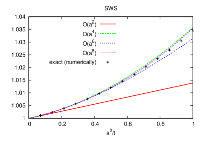
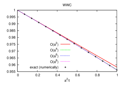
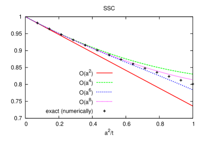
Figure 1: The tree-level improvement factor for four examples, the $SWS$, $WWC$, $SSS$ and $SSC$ cases, starting from only the $O(a^{2})$ correction and including higher and higher order terms. What is also shown is the all-order result obtained by numerically evaluating (17).

4 Improved gradient flow

Using the results from section 3 it is clear that the 3 free parameters $c_{f},c_{g},c_{e}$ (or equivalently $x,y,z$) can be tuned to achieve $O(a^{6})$ improvement in the Symanzik-Symanzik-Symanzik case. In the Symanzik-Symanzik-clover case only 2 free parameters are available, $c_{f},c_{g}$ (or equivalently $x,y$) and only $O(a^{4})$ improvement is possible.

The 3 parameters in the Symanzik-Symanzik-Symanzik case will allow setting $C_{2,4,6}=0$ and actually there are two separate sets of solutions. Substituting both of these into $C_{8}$ and picking the one which is minimal, leads to the improvement coefficients

$$c_{f} = -0.013993$$

$$c_{g} = 0.052556$$ (30)

$$c_{e} = 0.198078\;,$$

This choice corresponds to $O(a^{6})$ improvement at tree-level and even the next coefficient $C_{8}=0.0001253$ is quite small.

Similarly, in the Symanzik-Symanzik-clover case one may require $C_{2,4}=0$ and obtain

$$c_{f} = -0.012250$$ (31)

$$c_{g} = 0.099250$$

with $C_{6}=-0.0003022$, corresponding to $O(a^{4})$ improvement.

In actual simulations the gauge action used for generating the configurations is sometimes considered fixed and one only has control over the measurements. In these cases one may optimize the discretization of the flow and observable (i.e. $c_{f},c_{e}$) for the Symanzik-Symanzik-Symanzik case or the discretization of the flow only (i.e. $c_{f}$) for the Symanzik-Symanzik-clover case.

For example if $c_{g}=0$, i.e. the Wilson plaquette action was used for the simulation then,

$$c_{f} = 0$$

$$c_{e} = 3/16$$ (32)

will lead to $C_{2,4}=0$ and $C_{6}=7/20480$. As another example we quote the case of tree-level Symanzik improved gauge action for the simulation, i.e. $c_{g}=-1/12$ in which case the optimal improvement coefficients are

$$c_{f} = 0.0388441$$

$$c_{e} = 0.2206988$$ (33)

which again lead to $C_{2,4}=0$ and $C_{6}=-0.00131710$.

If the clover term is used for the observable and again $c_{g}$ is considered fixed, then setting $C_{2}=0$ is always possible leading to $O(a^{2})$ improvement. For arbitrary $c_{g}$ the optimal choice is

$$c_{f}=\frac{1}{48}-\frac{1}{3}c_{g}\;,$$ (34)

leading to $C_{4}=\frac{133}{240}c_{g}^{2}-\frac{7}{320}c_{g}-\frac{101}{30720}$.

5 Scale setting

The tree-level coefficients $C_{2m}$ can also be used for improving scale setting by both $t_{0}$ Luscher:2010iy and $w_{0}$ Borsanyi:2012zs . First, let us discuss scale setting by $t_{0}$. In this setup the quantity $F(t)=\langle t^{2}E(t)\rangle$ is set to a certain value $F_{0}$, usually $F_{0}=0.3$ in QCD, and the corresponding $t=t_{0}$ determines the scale, $1/\sqrt{t_{0}}\sim\Lambda_{QCD}$. Now one may improve on the scale determination by considering the improvement of $F(t)$ calculated in the previous sections. The improved scale setting condition is then

$$\frac{F(t_{0\,imp})}{1+\sum_{m=1}^{4}C_{2m}\frac{a^{2m}}{{t_{0\,imp}}^{m}}}=F_{0}\;,$$ (35)

which may be solved directly for $t_{0\,imp}$ using the numerically evaluated $F(t)$. It is instructive however to expand $t_{0\,imp}$ in the lattice spacing in order to see how small or large the effect of improvement is on this particular quantity.

To this end let us introduce coefficients $T_{2m}$ by

$$t_{0\,imp}=t_{0}\left(1+\sum_{m=1}^{4}T_{2m}\frac{a^{2m}}{t_{0}^{m}}\right)\;.$$ (36)

Clearly, $t_{0\,imp}$ needs to be expanded in $a^{2}/t_{0}$ according to (36) at two instances in (35), first in the argument of $F(t_{0\,imp})$ and second, in the denominator. The expansion then leads to the determination of the coefficients $T_{2m}$. In order to simplify notation let us introduce for the derivatives,

$$F^{\prime}_{0} = t\left.\frac{d}{dt}F(t)\right|_{t=t_{0}}$$

$$F^{\prime\prime}_{0} = t^{2}\left.\frac{d^{2}}{dt^{2}}F(t)\right|_{t=t_{0}}$$ (37)

$$F^{\prime\prime\prime}_{0} = t^{3}\left.\frac{d^{3}}{dt^{3}}F(t)\right|_{t=t_{0}}\;.$$

Using these the sought after improvement coefficients of $t_{0\,imp}$ are,

$$T_{2} = C_{2}\frac{F_{0}}{F^{\prime}_{0}}$$ (38)

$$T_{4} = C_{4}\frac{F_{0}}{F^{\prime}_{0}}-C_{2}^{2}\frac{F_{0}^{2}}{{F^{\prime}_{0}}^{3}}\left(F^{\prime}_{0}+\frac{1}{2}F^{\prime\prime}_{0}\right)$$

$$T_{6} = C_{6}\frac{F_{0}}{F^{\prime}_{0}}-C_{2}C_{4}\frac{F_{0}^{2}}{{F^{\prime}_{0}}^{3}}\left(3F^{\prime}_{0}+F^{\prime\prime}_{0}\right)+C_{2}^{3}\frac{F_{0}^{3}}{{F^{\prime}_{0}}^{5}}\left(2{F^{\prime}_{0}}^{2}+\frac{3}{2}F^{\prime}_{0}F^{\prime\prime}_{0}+\frac{1}{3}{F^{\prime\prime}_{0}}^{2}-\frac{1}{6}F^{\prime\prime\prime}_{0}F^{\prime}_{0}\right)\;.$$

The term $T_{8}$ is straightforward to calculate as well but will not be quoted here as it is quite lengthy. Note that in QCD the shape of $F(t)$ is roughly linear in $t$ for $t\sim t_{0}$ hence $F^{\prime\prime}_{0}$ and all further derivatives will be small.

A useful variant of scale setting by $t_{0}$ was introduced in Borsanyi:2012zs called $w_{0}$. In this setup the logarithmic derivative of $F(t)$ is set to a prescribed value $F^{\prime}_{0}$, again usually $F^{\prime}_{0}=0.3$ in QCD, and the corresponding $t=w_{0}^{2}$ value is used as scale, $w_{0}\sim 1/\Lambda_{QCD}$,

$$\left.t\frac{d}{dt}F(t)\right|_{t=w_{0}^{2}}=F^{\prime}_{0}\;.$$ (39)

In a completely analogous way as done for $t_{0}$ one may introduce the improved scale $w_{0\;imp}$ by

$$\left[t\frac{d}{dt}\frac{F(t)}{1+\sum_{m=1}^{4}C_{2m}\frac{a^{2m}}{t^{m}}}\right]_{t=w_{0\,imp}^{2}}=F^{\prime}_{0}\;,$$ (40)

which again can be solved directly. It is again instructive to expand $w_{0\,imp}^{2}$ in the lattice spacing,

$$w_{0\,imp}^{2}=w_{0}^{2}\left(1+\sum_{m=1}^{4}W_{2m}\frac{a^{2m}}{w_{0}^{2m}}\right)\;,$$ (41)

using another set of coefficients $W_{2m}$ which can be determined also analogously. When (40) is expanded one is lead to

$$W_{2} = C_{2}\frac{F^{\prime}_{0}-F_{0}}{F^{\prime\prime}_{0}+F^{\prime}_{0}}\;,$$ (42)

where of course the index $0$ refers to evaluating the function $F$ and its various derivatives at $t=w_{0}^{2}$. The further terms $W_{4,6,8}$ can also be easily calculated but are rather lengthy.

6 Finite volume

So far the calculations were performed on an infinite lattice. In Fodor:2012td the corresponding calculations in the continuum but finite volume were performed. In the present section we combine the two approaches and obtain results at finite lattice spacing and finite volume.

The gauge field is assumed to be periodic in all 4 directions and the result will have two distinct contributions, one coming from the zero modes and a second one from the non-zero modes. It can be shown that the contribution of the zero mode is the same in the continuum as at finite lattice spacing Coste:1985mn . This is intuitively clear because the zero mode is a constant and the 4-torus can just as well be considered a single point. In this case of course discretization effects cannot come into play. Hence only the contribution of the non-zero modes can be lattice spacing dependent. This contribution can easily be evaluated numerically by replacing the integral in our formula (17) by a discrete lattice sum over non-zero 4-momenta.

In this way we obtain the lattice spacing dependence of the finite volume correction factor $\delta(\sqrt{8t}/L)$ of Fodor:2012td where the ratio $\sqrt{8t}/L$ was called $c$ but in order not to introduce confusion with the improvement coefficients, $c$ will not be used for the ratio here. Equivalently, we obtain the finite volume dependence of the finite lattice spacing correction factor $C(a^{2}/t)$ of the present work,

$$C(a^{2}/t,\sqrt{8t}/L)=1+\delta(\sqrt{8t}/L,a/L)\;.$$ (43)

Specifically, using the formula (17) and the finite volume results from Fodor:2012td we obtain at finite lattice spacing and finite volume and leading order in the coupling,

$$\langle t^{2}E(t)\rangle = g^{2}\frac{3(N^{2}-1)}{128\pi^{2}}C(a^{2}/t,\sqrt{8t}/L)$$ (44)

$$C(a^{2}/t,\sqrt{8t}/L) = \frac{128\pi^{2}t^{2}}{3L^{4}}+\frac{64\pi^{2}t^{2}}{3L^{4}}\sum_{n_{\mu}=0,\;n^{2}\neq 0}^{L/a-1}{\rm Tr}\,\left(e^{-t\left({\cal S}^{f}+{\cal G}\right)}({\cal S}^{g}+{\cal G})^{-1}e^{-t\left({\cal S}^{f}+{\cal G}\right)}{\cal S}^{e}\right)\;,$$

where again the first term comes from the zero modes and is identical to the continuum result and $p_{\mu}=2\pi n_{\mu}/L$ with a non-zero integer 4-vector $n_{\mu}$. This expression can easily be evaluated numerically for any choice of discretizations.

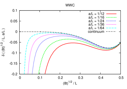
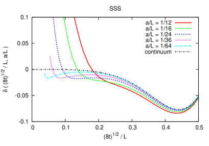
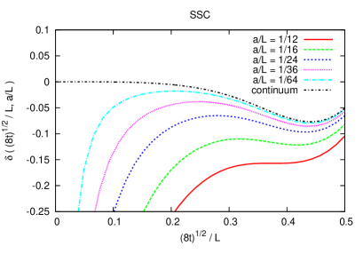
Figure 2: The tree-level finite volume and finite lattice spacing correction factors $\delta(\sqrt{8t}/L,a/L)=C(a^{2}/t,\sqrt{8t}/L)-1$ for four examples, the $SWS$, $WWC$, $SSS$ and $SSC$ cases as a function of $\sqrt{8t}/L$ at various lattice spacings. The continuum result is from Fodor:2012td .

For illustration we plot $\delta(\sqrt{8t}/L,a/L)=C(a^{2}/t,\sqrt{8t}/L)-1$ for four examples at various lattice volumes as a function of $\sqrt{8t}/L$ on figure 2. We also show the continuum result $\delta(\sqrt{8t}/L)$ from Fodor:2012td for comparison.

7 Numerical test

In order to test the numerical usefulness of our tree-level formulae we will consider the running coupling of $N_{f}=4$ flavors Fodor:2012td . For all details of the simulations we refer to the original work Fodor:2012td , here we simply quote two examples of continuum extrapolations that were performed there. At these and all the other renormalized couplings we computed the discrete $\beta$-function corresponding to a scale change of $s=3/2$ at various lattice spacings and performed continuum extrapolations.

Since the setup in Fodor:2012td is a step-scaling approach to the calculation of the $\beta$-function on a periodic 4-torus we need to use the finite volume, finite lattice spacing factor computed in the previous section.

For our numerical test the renormalized coupling in Fodor:2012td is tree-level improved by dividing by the tree-level expression $C(a^{2}/t,\sqrt{8t}/L)$ from (44) in the $SSC$ setup, i.e. tree-level Symanzik improved ($c=-1/12$) gauge action and flow with clover type observable with $\sqrt{8t}/L=3/10$, which was the setup used in the simulation. As it can be seen from figure 2 the continuum finite volume correction factor at $\sqrt{8t}/L=3/10$ is around 3% while the finite lattice spacing dependence can be 12% away from it for the smaller lattices while only about 1% away from it for the larger $L/a=36$ lattices.

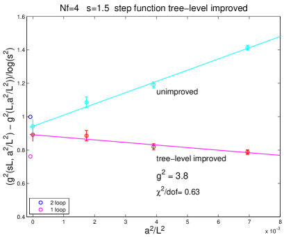
Figure 3: Continuum extrapolations of the discrete $\beta$-function for two selected $g^{2}$ values $1.4$ (left) and $3.8$ (right) for $N_{f}=4$ flavors with and without tree-level improvement. The data is from Fodor:2012td .

Figure 4: Parametrization of the tree-level improved renormalized coupling at fixed lattice sizes as a function of $\beta$ (left) and continuum extrapolated discrete $\beta$-function of $N_{f}=4$ flavors with a magnified section for better visibility (right). The data is from Fodor:2012td .

The resulting tree-level improved continuum extrapolations are shown in figure 3. Clearly, the slope of the extrapolation is greatly reduced by the improvement. The final error on the improved extrapolation is somewhat smaller than the unimproved version as expected.

Figure 4 shows the interpolation of the tree-level improved renormalized couplings on various lattice volumes as a function of $\beta$ and also the final continuum extrapolation for the discrete $\beta$-function for the full range of the renormalized couplings together with the 1-loop and 2-loop results. It should be noted though that the displayed error on the continuum result for the discrete $\beta$-function (figure 4, right) only includes statistical errors. Systematic effects so far have not been estimated.

8 Conclusion and outlook

The tree-level results obtained in this paper are useful for two reasons. First, if any simulation is performed with an arbitrary discretization the tree-level results can be used to tree-level improve the non-perturbative results by the corresponding tree-level expression. The necessary expressions were given for both finite and infinite volume setups. Such a tree-level improvement of course will not affect the continuum extrapolated result but will reduce the size of cut-off effects. Finite volume tree-level improvement was demonstrated to be useful for the calculation of the running coupling and the corresponding $\beta$-function.

Second, the tree-level analysis shows how to choose optimal discretizations for all three ingredients of the calculation: the gradient flow, the gauge action and the observable $E$, leading to $O(a^{6})$ improvement. If the discretization of the dynamical gauge action is considered fixed, $O(a^{4})$ improvement can be achieved.

A natural next step in the improvement program would be to calculate the 1-loop terms at finite lattice spacing which is beyond the scope of the present paper.

- (1)
- (2) M. Luscher, Commun. Math. Phys. 293, 899 (2010) [arXiv:0907.5491 [hep-lat]].
- (3) M. Luscher, JHEP 1008, 071 (2010) [arXiv:1006.4518 [hep-lat]].
- (4) M. Luscher, PoS LATTICE 2010, 015 (2010) [arXiv:1009.5877 [hep-lat]].
- (5) M. Luscher and P. Weisz, JHEP 1102, 051 (2011) [arXiv:1101.0963 [hep-th]].
- (6) S. Borsanyi, S. Durr, Z. Fodor, C. Hoelbling, S. D. Katz, S. Krieg, T. Kurth and L. Lellouch et al., JHEP 1209, 010 (2012) [arXiv:1203.4469 [hep-lat]].
- (7) A. Bazavov et al. [The MILC Collaboration], arXiv:1311.1474 [hep-lat].
- (8) R. Sommer, arXiv:1401.3270 [hep-lat].
- (9) Z. Fodor, K. Holland, J. Kuti, D. Nogradi and C. H. Wong, JHEP 1211, 007 (2012) [arXiv:1208.1051 [hep-lat]].
- (10) Z. Fodor, K. Holland, J. Kuti, D. Nogradi and C. H. Wong, PoS LATTICE 2012, 050 (2012) [arXiv:1211.3247 [hep-lat]].
- (11) P. Fritzsch and A. Ramos, JHEP 1310, 008 (2013) [arXiv:1301.4388 [hep-lat]].
- (12) P. Fritzsch and A. Ramos, arXiv:1308.4559 [hep-lat].
- (13) A. Ramos, arXiv:1308.4558 [hep-lat].
- (14) P. Fritzsch, A. Ramos and F. Stollenwerk, arXiv:1311.7304 [hep-lat].
- (15) J. Rantaharju, arXiv:1311.3719 [hep-lat].
- (16) M. Luscher, arXiv:1404.5930 [hep-lat].
- (17) M. Asakawa et al. [FlowQCD Collaboration], arXiv:1312.7492 [hep-lat].
- (18) O. Bar and M. Golterman, arXiv:1312.4999 [hep-lat].
- (19) H. Suzuki, PTEP 2013, no. 8, 083B03 (2013) [arXiv:1304.0533 [hep-lat]].
- (20) L. Del Debbio, A. Patella and A. Rago, JHEP 1311, 212 (2013) [arXiv:1306.1173 [hep-th]].
- (21) H. Makino and H. Suzuki, arXiv:1403.4772 [hep-lat].
- (22) M. Luscher, JHEP 1304, 123 (2013) [arXiv:1302.5246 [hep-lat]].
- (23) A. Shindler, Nucl. Phys. B 881, 71 (2014) [arXiv:1312.4908 [hep-lat]].
- (24) A. Cheng, A. Hasenfratz, Y. Liu, G. Petropoulos and D. Schaich, arXiv:1404.0984 [hep-lat].
- (25) P. Weisz, Nucl. Phys. B 212, 1 (1983).
- (26) K. Symanzik, Nucl. Phys. B 226, 187 (1983).
- (27) P. Weisz and R. Wohlert, Nucl. Phys. B 236, 397 (1984) [Erratum-ibid. B 247, 544 (1984)].
- (28) M. Luscher and P. Weisz, Commun. Math. Phys. 97, 59 (1985) [Erratum-ibid. 98, 433 (1985)].
- (29) M. Luscher and P. Weisz, Phys. Lett. B 158, 250 (1985).
- (30) A. Coste, A. Gonzalez-Arroyo, J. Jurkiewicz and C. P. Korthals Altes, Nucl. Phys. B 262, 67 (1985).