Two paths of cluster evolution: global expansion versus core collapse

Abstract

All gravitationally bound clusters expand, due to both gas loss from their most massive members and binary heating. All are eventually disrupted tidally, either by passing molecular clouds or the gravitational potential of their host galaxies. However, their interior evolution can follow two very different paths. Only clusters of sufficiently large initial population and size undergo the combined interior contraction and exterior expansion that leads eventually to core collapse. In all other systems, core collapse is frustrated by binary heating. These clusters globally expand for their entire lives, up to the point of tidal disruption.

Using a suite of direct $N$-body calculations, we trace the “collapse line” in $r_{v}-N$ space that separates these two paths. Here, $r_{v}$ and $N$ are the cluster’s initial virial radius and population, respectively. For realistic starting radii, the dividing $N$-value is from $10^{4}$ to over $10^{5}$. We also show that there exists a minimum population, $N_{\rm min}$, for core collapse. Clusters with $N<N_{\rm min}$ tidally disrupt before core collapse occurs. At the Sun’s Galactocentric radius, $R_{G}=8.5$ kpc, we find $N_{\rm min}\gtrsim 300$. The minimum population scales with Galactocentric radius as $R_{G}^{-9/8}$.

The position of an observed cluster relative to the collapse line can be used to predict its future evolution. Using a small sample of open clusters, we find that most lie below the collapse line, and thus will never undergo core collapse. Most globular clusters, on the other hand, lie well above the line. In such a case, the cluster may or may not go through core collapse, depending on its initial size. We show how an accurate age determination can help settle this issue.

1 Introduction

In the classic theory of cluster evolution, the interior region contracts and transfers energy through distant two-body encounters to an expanding outer halo. This process of relaxation is a consequence of the negative heat capacity of self-gravitating systems. Eventually, the rise of central density becomes dramatic, an event known as the gravothermal catastrophe (Lynden-Bell & Wood, 1968). The system at this epoch is commonly said to undergo core collapse.

For a hypothetical cluster comprised of identical, single stars, numerical simulations find that core collapse occurs after more than ten relaxation times (Cohn, 1980; Makino, 1996). The catastrophe ends when a tight binary forms near the center. Binary heating then not only halts the rise in central density, but leads to a global expansion of the system (Hénon, 1965; Aarseth, 1971). Observationally, a substantial fraction of the most massive globular clusters ($M_{\rm cl}\gtrsim 10^{5}\,{\rm M}_{\odot}$) exhibit a central peak in stellar density and luminosity, and are thought to have undergone core collapse in the past (Djorgovski & King, 1986; Trager, King & Djorgovski, 1995; Meylan & Heggie, 1997).

Of course, the member stars of real clusters are not identical. Globular clusters are so old that stellar evolution has pared down the initial mass distribution to a relatively narrow range. In this case, the classic theory provides a reasonably accurate description at sufficiently late times. The vast majority of clusters in the Milky Way are open clusters, which are much less populous and do not live nearly as long as globular clusters (Röser et al., 2010). The evolutionary path of these more modest systems may be strikingly different.

Regardless of the cluster’s precise initial state, its most massive stars quickly sink to the center through dynamical friction. This mass segregation occurs in less than a single relaxation time (e.g., Gürkan, Freitag & Rasio, 2004, and references therein). Three-body encounters between the central stars soon create a few massive binaries, whose heating frustrates the process of core contraction (Converse & Stahler, 2011; Tanikawa, Hut & Makino, 2012). In systems of relatively low population and size, core collapse never occurs.

In this paper, we explore these two, very different evolutionary paths. We first delineate the boundary between the two paths using an analytic argument. We then verify the location of that boundary and describe the structural evolution of clusters on either side of it numerically. Here, we employ the direct $N$-body integrator nody6-gpu (Aarseth, 1999; Nitadori & Aarseth, 2012). Our simulations span a population range from about $8\times 10^{3}$ to over $1\times 10^{5}$ so that we may characterize the evolution of both open and globular clusters. Our simulations include a realistic mass distribution, stellar evolution, and the influence of the Galactic tidal field.

Our combined analytical and numerical results show that a cluster must be relatively large and populous to undergo core collapse. Because of the external tidal field, the evolution of any system also depends on its location relative to the Galactic center. For any fixed location, there exists a minimum population such that sparser clusters never undergo collapse, regardless of their exact initial state. We again verify the existence of this minimum population both analytically and numerically.

A number of previous studies also investigated cluster evolution through a suite of simulations. In some cases, the researchers included populations as high as our maximum value (e.g., Baumgardt & Makino, 2003; Zonoozi et al., 2011). These projects addressed a variety of specific issues, such as how metallicity effects the changing appearance of clusters (Sippel et al., 2012). Baumgardt & Makino (2003) presented the most extensive, simulation-based investigation to date, focusing primarily on how the stellar mass function scales with time. Ours is a complementary study, intended to establish the broad landscape in which clusters evolve.

This work is organized as follows. In § 2, we analyze the relevant timescales for the competition between mass segregation, relaxation, and stellar mass loss in clusters. We describe our numerical simulations in § 3 and present the bulk of our results in § 4. Finally, we summarize and discuss the implications of our results in § 5.

2 The collapse line

We focus here on the cluster’s evolution after the first few dynamical times since its formation within a molecular cloud. By that point, radiation pressure and energetic winds from the most massive stars have dispersed all cloud gas, leaving the stars to interact only via their mutual gravity. Subsequently, the bulk of the cluster steadily expands, until the system is ultimately disrupted tidally, either by passing molecular clouds or the Galactic field. The central issue we address is the fate of the cluster’s deep interior.

The evolution of this central core is driven by the competition of dynamical cooling and heating (see, e.g., Hénon, 1961). On the one hand, the core transfers energy outward to the halo stars through two-body relaxation, and thereby tends to contract. On the other hand, a single hard binary near the center of the cluster may effectively heat the core through three-body interactions, causing it to expand. The core contains a large fraction of the cluster’s most massive stars. In the course of stellar evolution, mass loss from these objects in the form of stellar winds and supernovae diminishes the gravitational binding of the core, again promoting expansion.

Consider first a hypothetical cluster of mass $M_{\rm cl}$ containing $N$ identical stars. Here, the central core transfers energy outward through two-body encounters. This transfer occurs on $t_{\rm rel}$, the initial relaxation time scale

$$t_{\rm rel}=\frac{0.17N}{\ln(0.1N)}\sqrt{\frac{r_{v}^{3}}{GM_{cl}}},$$ (1)

which we define at the virial radius, $r_{v}$ (cf. Binney & Tremaine, 2008, eq. 7.108). We take the virial radius to be $r_{v}\equiv GM_{cl}/6\sigma^{2}$, where $\sigma$ is cluster’s one-dimensional velocity dispersion. When tracking $r_{v}$ in our simulations, we determined $\sigma$ directly from the stellar velocities at each time step.

While the uniform-mass cluster can, in principle, form binaries, the time to do so is several hundred $t_{\rm rel}$ (Binney & Tremaine, 2008, eq. 7.12). Long before this, the cluster’s central density rises, eventually in a divergent manner in a finite time. Numerical simulations suggest that this core collapse occurs at $t_{cc}\approx 16t_{\rm rel}$ (Cohn, 1980; Makino, 1996). Despite the idealized assumption underlying this picture, it is still frequently used as the framework to describe the evolution of all clusters.

Realistic clusters have a broad spectrum of stellar masses. The most massive stars, whatever their initial location, migrate toward the center as a result of dynamical friction. For a star with mass $m_{*}\gg\left<m\right>$, this process occurs over the dynamical friction time $t_{df}$, which is brief compared to $t_{\rm rel}$:

$$t_{df}\approx\frac{\left<m\right>}{m_{*}}t_{\rm rel}.$$ (2)

Here, $\left<m\right>$ is the cluster’s average stellar mass (Fregeau et al., 2002). Both the mass density and average stellar mass in the core are thereby enhanced.

Since the relaxation time in the core is smaller than that of the cluster as a whole, the core effectively decouples from the rest of the system, and evolves separately, a process known as the Spitzer (1969) instability. For decoupling to occur, a sufficient number of massive stars must migrate to the cluster center, forming a subgroup whose dynamical temperature, proportional to the mean value of $m\sigma^{2}$, rises above that of surrounding stars. The time required for decoupling, $t_{\rm dec}$, depends on the density profile of the cluster and the degree of primordial mass segregation (e.g., Quinlan, 1996; Vesperini, McMillan & Portegies Zwart, 2009). A representative value, adequate for our purpose, is $t_{\rm dec}=2\,t_{df}$.

One significant result of the core’s fast evolution is the formation of hard binaries consisting of relatively massive stars. These binaries are created through three-body interactions. Their formation time is very sensitive to the largest mass involved, and scales approximately as $m_{*}^{-10}$ (Ivanova et al., 2005; Converse & Stahler, 2011). Very soon after decoupling, at least one massive binary forms, heats the core through three-body interactions, and creates global expansion of the cluster. This binary can be disrupted or ejected from the cluster; however, a new one soon replaces it (Heggie & Hut, 2003).

In a cluster of sufficiently high population, stellar evolution prevents the formation of massive binaries in the core. Let $t_{\rm ms}$ represent the main-sequence lifetime of the most massive stars. As we consider clusters of larger $N$ and comparable size, both $t_{\rm rel}$ and $t_{\rm dec}$ grow. When $t_{\rm dec}$ exceeds $t_{\rm ms}$, the most massive stars explode as supernovae before they can migrate to the center and form binaries. It is true that the disappearance of massive stars already located in the core temporarily heats the cluster, but eventually, the region begins to contract via two-body relaxation. These populous, aging clusters have a relatively narrow mass distribution, and evolve toward core collapse in a manner similar to that of traditional theory.

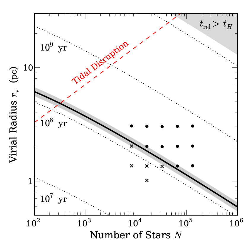
Figure 1: The collapse line in the $r_{v}$-$N$ plane. Clusters starting above the solid curve undergo core collapse if they survive long enough. Those starting below this curve never experience core collapse. Finally, clusters starting above the diagonal, dashed line are tidally disrupted at a Galactocentric distance of 8.5 kpc. Each dotted, diagonal line represents the indicated relaxation time $t_{\rm rel}$. Clusters in the upper, shaded region have $t_{\rm rel}$ greater than $t_{H}$, the Hubble time, and so never relax. The shading around the solid curve shows the range of values it may take depending on the clusters’ precise initial conditions. The discrete symbols show the initial conditions of our simulations. Crosses represent clusters that failed to achieve core collapse, while filled circles are clusters whose central number density eventually increased.

We see that the condition $t_{\rm dec}\approx t_{\rm ms}$ represents a dividing line between clusters that can undergo core collapse and those that cannot. If we elevate this condition to an exact equality, then equations (1) and (2) may be used to solve for $r_{v}$ in terms of $N$,

$$r_{v}^{3/2}=2.9\,t_{\rm ms}\sqrt{G\left<m\right>}\frac{m_{*}}{\left<m\right>}\frac{\ln(0.1N)}{\sqrt{N}}.$$ (3)

In this equation $m_{*}$ is the upper limit to the stellar mass. Any star with $m_{*}\gtrsim 10{\rm M}_{\odot}$ has a $t_{\rm ms}$ shorter than $2\times 10^{7}$ yr, a time approaching that during which the cluster was still embedded in its parent molecular cloud. If we choose $m_{*}=10\,{\rm M}_{\odot}$ and a minimum mass of $0.1\,{\rm M}_{\odot}$, then the average mass is $\left<m\right>\approx 0.6\,{\rm M}_{\odot}$ for the initial mass function of Miller & Scalo (1979). Setting $t_{ms}=2\times 10^{7}$ yr we find the collapse line:

$$r_{\rm coll}=2\left(\frac{6.9+\ln{N_{4}}}{6.9\sqrt{N_{4}}}\right)^{2/3}{\rm pc},$$ (4)

where $N_{4}\equiv N/10^{4}$, and $6.9=\ln{(10^{3})}$. We plot equation (4) as the solid line in Figure 1. The dotted, diagonal lines in the figure represent the indicated values of $t_{\rm rel}$. Systems within the shaded region in the upper right corner can never relax, since $t_{\rm rel}$ exceeds the Hubble time, $t_{H}=14\,$Gyr.

In numerically evaluating the right side of equation (3), we have made certain definite, but somewhat arbitrary, choices. For example, the literature offers a number of prescriptions for the field-star initial mass function. Using the Kroupa & Weidner (2003) initial mass function with the same upper and lower bounds for the stellar mass would reduce $\left<m\right>$ to $0.45\,{\rm M}_{\odot}$ and thus shift the collapse line in Figure 1 to the right by $\Delta\log{N}\approx 0.12$, while preserving its slope. Retaining the Miller & Scalo initial mass function, but increasing $m_{*}$ by a factor of two would lower $t_{\rm ms}$ to $1\times 10^{7}\,$yr, still a reasonable estimate for the embedded duration. Since the product $(t_{\rm ms}m_{*})$ is insensitive to $m_{*}$ in this regime, the collapse line would shift only slightly to the left. Primordial mass segregation and variations in the initial density profile of the cluster introduce a similar amount of uncertainty. It is therefore more accurate to envision the collapse line we plotted in Figure 1 as a narrow band of total width $\Delta\log{N}\approx 2\log{\Delta\left<m\right>}\approx 0.2$. We indicate this band by light shading in the figure.

3 $N$-body Simulations

In this work, we have performed an extensive suite of $N$-body simulations using the direct $N$-body integrator nody6-gpu (Aarseth, 1999; Nitadori & Aarseth, 2012) accelerated with graphics processing units. Our simulations include both single and binary star evolution, treating mass loss as an instantaneous process (Hurley, Pols & Tout, 2000; Hurley, Tout & Pols, 2002). We also include a representation of the Galactic tide, as described below. We focus on the evolution of star clusters after the primordial gas has been removed from the system by both low-mass stellar outflows and by the ionization and winds from massive stars.

We initialize our clusters with single stars distributed in a Plummer (1911) potential,

$$\phi_{\rm pl}(r)=-\frac{GM_{\rm cl}}{\sqrt{r^{2}+a^{2}}},$$ (5)

where $a=(3\pi/16)r_{v}\approx 0.59\,r_{v}$ is the Plummer radius and $M_{cl}=N\left<m\right>$. The mass of each star is then selected between $0.1\,{\rm M}_{\odot}$ and $10\,{\rm M}_{\odot}$ following the initial mass function of Miller & Scalo (1979). After generating the stellar distribution, the masses are rescaled so that the maximum stellar mass is exactly $10\,{\rm M}_{\odot}$, with $\left<m\right>\approx 0.6\,{\rm M}_{\odot}$. For simulations with a fixed $N$, both the masses of all stars and their positions scaled to the virial radius are identical, to reduce the stochastic noise. No initial mass segregation is imposed.

The early evolution of a cluster depends in detail on the fraction and spatial distribution of primordial binaries (see, e.g., Portegies Zwart, McMillan & Makino, 2007; Trenti, Heggie & Hut, 2007). Rather than explore this dependence, we have chosen to start all runs with single stars only. This choice gives us a uniform set of initial conditions and, in any case, has little practical effect on the subsequent evolution. As has been shown in previous studies (e.g., Tanikawa, Hut & Makino, 2012), and as we verify, central binaries rapidly form after the more massive cluster members drift to the center via dynamical friction.

We select the cluster virial radii $r_{v}$ and sizes $N$ to cover the transition in evolutionary path from global expansion to core collapse for systems similar to those observed in the Milky Way. In Figure 1, we show the initial conditions for 16 of our simulations which bracket the collapse line (eq. 4). The clusters have populations $N$ starting from 8,192 and increasing, by a factor of two, to a maximum of $N=$131,072. The minimum $r_{v}$-value, used only in conjunction with $N=$16,384, was 1.0 pc. For all other $N$-values, we used $r_{v}$ = 1.3, 2.0, and 3.0 pc. The upper limit for $N$ was chosen for practical reasons. Simulations with $N=131,072$ took a few weeks to complete on a single desktop with a GPU. Increasing the cluster population even by a factor of two would have required several months per run.

The clusters evolve in a spherical tidal gravitational field similar to that experienced by Milky Way clusters on circular orbits. Specifically, we adopt an isothermal potential with a constant circular velocity, $v_{c}=220\,{\rm km\,s}^{-1}$. With this potential, there is an enclosed mass of ${M_{\rm enc}=9.6\times 10^{10}(R_{G}/8.5\,{\rm kpc})\,{\rm M}_{\odot}}$ within an orbit of radius $R_{G}$. Unless otherwise noted, all simulations assume the clusters follow a circular orbit of radius $8.5\,$kpc. Stars are removed from our simulations when they are outside of $2r_{t}$, where $r_{t}$ is the tidal radius:

$$r_{t}\equiv R_{G}(M_{\rm cl}/2M_{\rm enc})^{1/3}.$$ (6)

For our models, the value of $r_{t}$ ranges from $20$ to $60\,$pc.

We run all of our simulations for a minimum of $15\,t_{\rm rel}$. If the cluster does not exhibit core collapse by $t=15\,t_{\rm rel}$, we continue the simulations until the system loses at least $90\%$ of its initial population. In none of these cases did core collapse occur before the cluster dissolved.

4 Results & Analysis

As first envisioned, core collapse occurs when the central density of a cluster rises in a sharply accelerating manner. Such behavior was first predicted theoretically (Hénon, 1961; Lynden-Bell & Wood, 1968), then clearly exhibited in both fluid models of clusters (Larson, 1970) and in $N$-body simulations of idealized systems comprised of identical-mass stars (e.g., Aarseth, Hénon & Wielen, 1974; Makino, 1996). In these cases, there is no ambiguity in defining the central density or describing its temporal change. However, subtleties arise when analyzing modern simulations that follow the dynamics of a stellar population spanning a realistic distribution of masses.

Our main goal is to give an account of cluster evolution that will prove useful when considering real, observed systems. These are only seen in projection against the plane of the sky. Hence, we begin by discussing the evolution of the projected, two-dimensional central number density, ${\cal N}_{\rm o}$. We focus on the number, rather than mass density, since the latter may change because of local processes, such as stellar mass loss via winds. We defer discussion of three-dimensional effects to the following subsection. There we also view our results within an alternative framework that is also frequently employed — the evolution of the cluster’s core radius.

4.1 Evolution of the projected central density

Before even choosing an operationally suitable definition of ${\cal N}_{\rm o}$, we must first be able to locate with precision the cluster’s center. Following von Hoerner (1960), we first associate a local surface density ${\cal N}_{i}$ with each cluster member, excluding escapers, here labeled by the index $i$. This member can be a single star or a binary. To establish each ${\cal N}_{i}$, we use the area spanned by the object’s 7 nearest neighbors (Casertano & Hut, 1985). Then, relative to any convenient origin, the cluster center is the density-weighted average position vector of all the members:

$${\bm{R}_{\rm o}}=\frac{\sum_{i}{\bm{R}_{i}}{\cal N}_{i}}{\sum_{i}{\cal N}_{i}},$$ (7)

For cluster members that are binaries, ${\bm{R}_{i}}$ locates the center of mass of the pair. Note again that all vectors are two-dimensional.

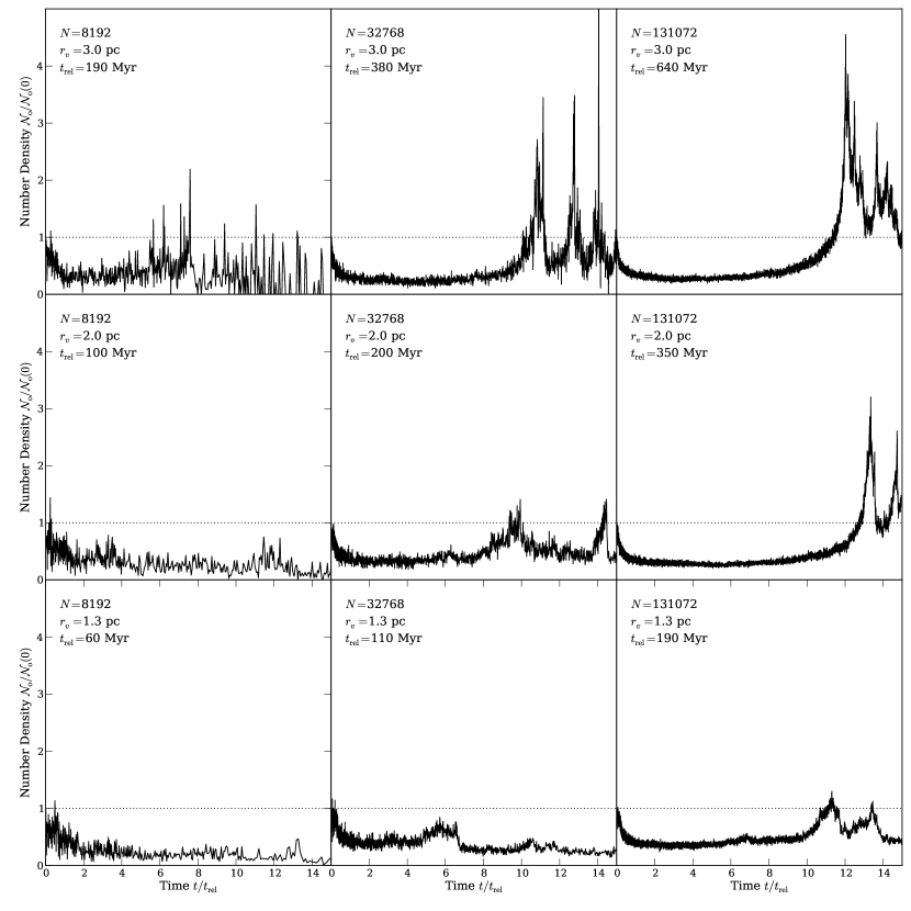
Figure 2: Normalized central surface number density. We plot the central projected number density of stars within $0.01R_{h}$, ${\cal N}_{\rm o}$, normalized by the initial density, ${\cal N}_{\rm o}(0)$, as a function of time for nine of our simulations. The number of stars, $N$, and virial radius, $r_{v}$, of each cluster is labeled in the panel. Also labeled is the initial relaxation time, $t_{\rm rel}$. The dashed line shows the threshold for core collapse. In general, the depth of the collapse increases with $N$ (from left to right) and $r_{V}$ (from bottom to the top). Only the clusters above the collapse line (see Fig. 1), however, undergo core collapse.

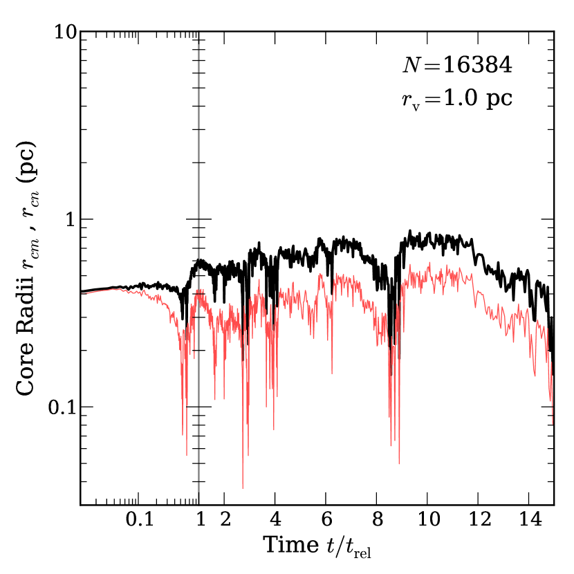
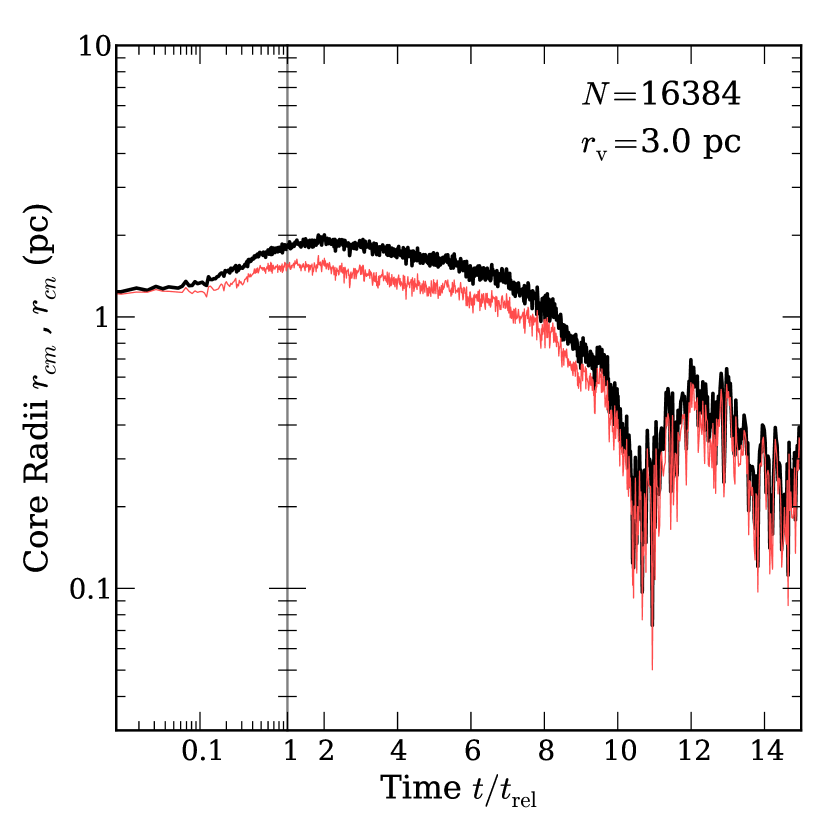
Figure 3: Evolution of the core radii $r_{cn}$ and $r_{cm}$ for a cluster that does not undergo core collapse (left panel) and one that does (right panel). In both cases, the number-weighted radius $r_{cn}$ is the thicker curve that is higher in the plot. As in Figure 2, we measure time relative to the initial value of $t_{\rm rel}$. Note the scale of the horizontal axis changes from logarithmic to linear at $t/t_{\rm rel}=1$.

Having located the center, we find ${\cal N}_{\rm o}$ by counting up the cluster members within a concentric circle. If the circle is chosen to enclose a fixed and relatively small number of stars, eg, 7 or 70, then the defined ${\cal N}_{\rm o}$ undergoes large Poisson fluctuations. In addition, the adopted radius should scale with the total cluster population $N$, which varies widely in our suite of simulations. Let $R_{h}$ be the radius containing, at any time, half the total members. If $f$ is a number less than unity, then the central density ${\cal N}_{\rm o}$ is defined as the number of stars within the radius $fR_{h}$, divided by the corresponding surface area. Choosing an $f$-value that is relatively high (e.g., 0.1) smears out the evolution. We have found in practice that $f=0.01$ yields an ${\cal N}_{\rm o}$ that exhibits a smooth evolution while retaining easily discernible trends. Obviously, there is some latitude in this definition; changing $f$ by a factor of two or so in either direction makes no appreciable difference in the resulting ${\cal N}_{\rm o}(t)$, except for the amount of noise in the results.

To undergo core collapse, the cluster should exhibit an accelerating rise in central density. In particular, we define core collapse to occur when the central density of the cluster exceeds its initial density,

$$\frac{{\cal N}_{\rm o}}{{\cal N}_{\rm o}(0)}>1.$$ (8)

In Figure 2, we plot ${\cal N}_{\rm o}$ as a function of time for nine runs. Here we have normalized ${\cal N}_{\rm o}$ by ${\cal N}_{\rm o}(0)$, and the time $t$ by the initial value of $t_{\rm rel}$. All clusters with an initial $r_{v}$ of $3.0\,$pc (top row) undergo core collapse, according to our criterion. Of clusters starting with $r_{v}=2.0\,$pc (middle row), those two with $N\geq 32768$ undergo collapse. Finally, of the clusters with $r_{v}=1.3\,$pc (bottom row), only that with the highest $N$ reaches this state. In all these cases, the initial parameters of the clusters place them above the collapse line in Figure 1. These systems have relatively large $N$ and most closely mimic the behavior of uniform-mass clusters.

In all such runs, we see that the central density, after exceeding its initial value, later plunges below it and then climbs again. If the simulation were extended to longer times, this pattern would repeat. Such “gravothermal oscillations” are caused by the successive formation and ejection of central binaries. The phenomenon has long been documented in the theoretical literature on equal-mass systems (Bettwieser & Sugimoto, 1984; Goodman, 1984).

In contrast to this behavior is that of clusters with $t_{\rm dec}<t_{\rm ms}$, i.e., those starting below the collapse line in Figure 1. In these, the central density never exceeds its initial value, except perhaps transiently early in the evolution. (Such excursions last about one dynamical time.) These systems undergo global expansion, as was found in the simulations of Converse & Stahler (2011), and as we will show in more detail below. In Figure 1, we have marked the model clusters that undergo core collapse with filled circles, and those exhibiting global expansion with crosses. It is evident that the collapse line indeed demarcates the two distinct evolutionary paths.

The maximum normalized central density attained by a cluster increases with both $N$ and $r_{v}$, from the bottom left to the top right in Figure 2. Graphically, the systems that reach the highest central density during core collapse are farthest above the collapse line. For systems lying close to the line, relatively small changes in $N$ or $r_{v}$ can result in the central density either falling a bit below or slightly above its initial value. In such marginal cases, it is unclear whether the cluster should be deemed as undergoing core collapse. Further, we have noted that our operational definition of the central density itself is somewhat arbitrary. These factors introduce additional uncertainty in the true location of the collapse line, but the induced width is small compared to that arising from initial conditions, as outlined in Section 2.

4.2 Three-dimensional evolution: Core radius

We gain a better physical understanding of the cluster’s behavior by examining it not just in projection, but in three-dimensional space. The extensive literature in this field has focused traditionally on the evolution of the core radius, again defined three-dimensionally. It is instructive to view our main result in this perspective, both to place it in the context of previous research, and to further elucidate the two evolutionary paths.

As in Section 4.1, we must first establish the cluster center, this time in three dimensions. We again follow von Hoerner (1960) and Casertano & Hut (1985), using the 7 nearest neighbors to assign a local, volumetric number density $n_{i}$ to each cluster member. We identify the cluster’s center as the density-weighted average position vector of all members:

$${\bm{r}}_{{\rm o}n}=\frac{\sum_{i}{\bm{r}_{i}}{n}_{i}}{\sum_{i}{n}_{i}}.$$ (9)

Note that the additional “$n$” subscript specifies our use of number densities in the weighting. We define a number-weighted core radius, denoted $r_{cn}$, by finding the average distance of members from the center, again weighted by the local number density:

$$r_{cn}=\frac{\sum_{i}|{\bm{r}_{i}-\bm{r}_{{\rm o}n}}|{n}_{i}}{\sum_{i}{n}_{i}}.$$ (10)

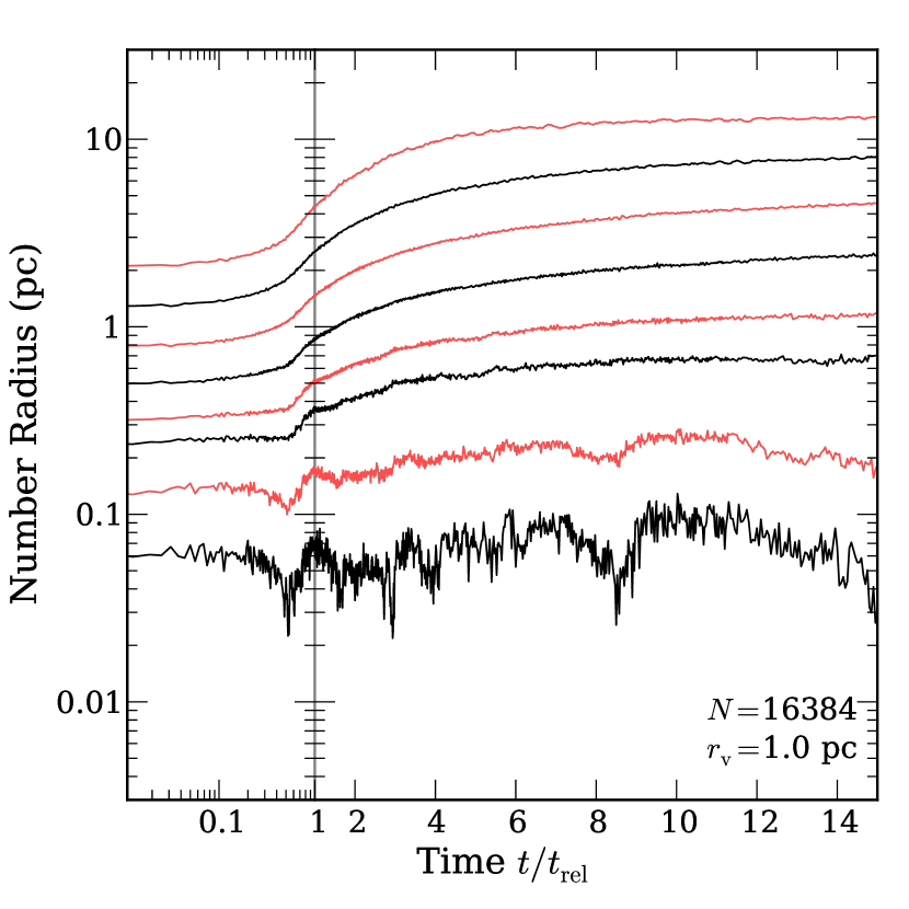
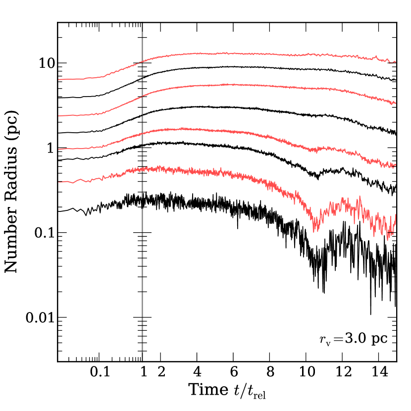
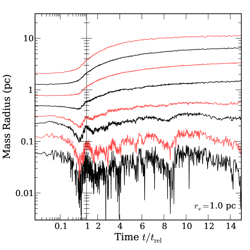
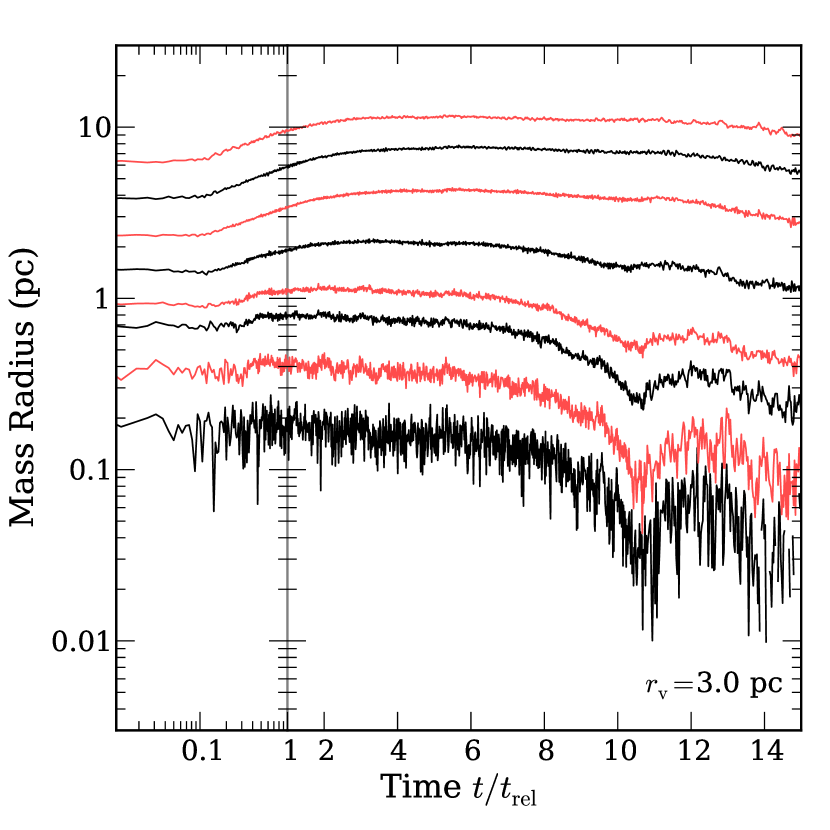
Figure 4: Evolution of the number radii (top row) and mass radii (bottom row) for a cluster with $N=$16,384. For a starting virial radius of $r_{v}=1.0\,$pc, the cluster does not undergo core collapse, while it does for $r_{v}=3.0\,$pc. Within each panel the displayed Lagrangian radii enclose a fraction $f=0.001,0.01,0.05,0.10,0.25,0.50,0.75,$ and $0.90$ of the cluster’s total population or mass. Note again that the scale of the horizontal axis changes from logarithmic to linear at $t/t_{\rm rel}=1$, where $t_{\rm rel}$ is the initial relaxation time.

Our definitions of the cluster center and core radius follow those in the literature, but with one difference. Traditionally, the weighting factor is the mass density $\rho_{i}$ associated with each member. Using $\rho_{i}$ instead of $n_{i}$, we may alter equations (9) and (10) to define the analogous mass-weighted central position vector, $r_{{\rm o}m}$, and core radius, $r_{{\rm c}m}$. It is also traditional to track the evolution of the cluster’s tidal radius, $r_{t}$. Beyond this radius, a star escapes the cluster if the system is on a circular orbit around the Galactic center. When

$$\frac{r_{cm}}{r_{t}}\leq 10^{-2},$$ (11)

the cluster is traditionally said to undergo core collapse (e.g., Makino 1996, Gürkan, Freitag & Rasio 2004, and Portegies Zwart, McMillan & Makino 2007).

For the evolution of an idealized, single-mass cluster, the number and mass densities are proportional at all times. Hence $r_{cm}=r_{cn}$. In this case, simulations find that the cluster’s interior density eventually exhibits a power-law profile. That is $n(r)\propto r^{-p}$, where $r$ is the distance from the center and the exponent $p\approx 2.2$ (see, e.g., Cohn, 1980). At this epoch, the core radius, as defined by equation (10), shrinks to zero, and the traditional criterion for core collapse, equation (11), is satisfied.

In more realistic systems containing a range of stellar masses, the two definitions of core radius are not equivalent. The behavior of $r_{cn}(t)$ and $r_{cm}(t)$ is more complex and interesting than in single-mass models. Figure 3 displays the evolution of the two quantities for two simulations that lie on either side of the collapse line with $N=16,384$. In the left panel (with $r_{v}=1.0\,$pc), which shows a cluster that does not undergo core collapse, $r_{cn}(t)$ exhibits fluctuations, but does not deviate by more than a factor of a few from its value at $t=t_{\rm rel}$.

On the other hand, $r_{cm}(t)$ does have several dramatic plunges. These are the result of mass segregation. At each time, a few members of especially large mass have drifted to the center via dynamical friction. These members couple with others to form the binaries which cause the cluster to expand, but they do not substantially increase the central number density. The first such event occurs in less than a single relaxation time, as can be seen in the left portion of the panel. The stars in question contribute a small fraction of the cluster’s total mass (Gürkan, Freitag & Rasio, 2004), and a much smaller fraction of the total number of stars. In this simulation, fewer than ten stars are involved in the contraction of $r_{cm}$.

The right panel of Figure 3 displays the evolution of $r_{cn}$ and $r_{cm}$ for a cluster that does undergo core collapse, with $r_{v}=3.0\,$pc. Here, there are no early plunges of $r_{cm}(t)$ associated with mass segregation, since the most massive stars die before they can reach the center. The two core radii now track each other closely. In particular, both take a sharp drop at $t\approx 11\,t_{\rm rel}$, which marks the epoch of the first core collapse, according to our definition. By this point, the cluster’s mass spectrum has narrowed considerably from the initial state, just as in observed globular clusters. The fraction of cluster mass within $r_{cm}$ at the formation of the first binary is similar to the simulation in the left panel.

4.3 Three-dimensional evolution: Lagrangian radii

We gain a more detailed understanding of the cluster’s behavior by following the evolution of its interior density. Traditionally, researchers have considered spherical shells that contain a fixed fraction of the system’s total current mass. Here, we will follow this convention, and thus trace the radii of individual mass shells. However, we are also interested in shells that contain a fixed fraction of the current, total population. A “number radius” containing, e.g., 10 percent of the population, does not generally contain 10 percent of the cluster mass. Indeed, the differing evolutions of the number and mass radii provide further insight into the nature of the two evolutionary paths of the cluster and the impact of mass segregation.

Figure 4 displays the evolution of selected number and mass radii for the same two clusters as in Figure 3, i.e., systems lying on either side of the collapse line. The top two panels show number radii for both clusters. The one starting with $r_{v}=1.0\,$pc lies below the collapse line. Here, the number radii generally expand with time. It is only the innermost shell, containing 0.001 of the current population, that has repeated dips in its radius. These dips are associated with binary formation by massive stars, as discussed in Section 4.2. Note that the shell in question contains at most 17 stars. Only on this tiny scale does a number radius ever decrease significantly. In contrast, 95 percent of the cluster population expand monotonically from the start, as exemplified by the shell containing 5 percent of the cluster population.

The top right panel traces the evolution of number radii for the cluster starting with $r_{v}=3.0\,$pc and lying above the collapse line. In this case, the number radii in the deep interior evolve more smoothly, since there are no repeated dips associated with massive binary formation. All radii eventually contract, and the interior ones plunge steeply at $t=11\,t_{\rm rel}$, the time of core collapse.

We get a very different impression when we examine the mass radii for the same systems. The bottom two panels show mass radii for the same two clusters. For the one with an initial $r_{v}$ of $1.0\,$pc, several radii have repeated, sharp plunges, much steeper than those of the analogous number radii. Each plunge occurs when a few massive stars drift to the center. The first such event coincides with the formation of the first hard binary. At this point, the interior mass shell comprising 1 percent of the cluster mass contracts by an order of magnitude and contains only 7 stars. Just afterward, all mass shells rapidly enlarge, a manifestation of binary heating.

Another traditional criterion for core collapse is the contraction of interior mass shells (e.g., Giersz & Heggie, 1997; Gürkan, Freitag & Rasio, 2004). We now see that mass segregation, and not the global relaxation of the cluster, may be responsible for this contraction. In the present case, only the innermost 50 percent of the cluster’s mass expands for the entire run. At the same time, the physical spacing between almost all stars, except a very few near the center, steadily increases. Thus, the system truly undergoes global expansion. The net efflux of stars from the central region accounts for the fact that the core radius $r_{cn}(t)$ stays roughly constant, as noted previously.

In the bottom right panel, we see the evolution of mass shells in the cluster that is initially larger. For this system, the mass and number radii track each other quite closely, i.e., there is little sign of mass segregation. Again, there are no deep plunges of shells early in the evolution. Massive stars that drift to the center during that epoch die out before reaching it. When contraction finally does occur, it involves interior number and mass shells. At this point, about 10 percent of the cluster’s total population and mass participate in the contraction. There is large-scale energy transfer from the interior to the outside, as documented numerically by Converse & Stahler (2011). Contraction again ends with central binary formation and subsequent rapid expansion.

4.4 Expansion and tidal disruption

In both clusters shown in Figures 3 and 4, the bulk expansion just after formation of the first binary exhibits power-law behavior. Thus, the virial radius $r_{v}$ scales as $(t-t_{o})^{p}$, where $t_{o}$ is the appropriate binary formation time. Hénon (1965) showed that such homologous expansion is expected whenever the cluster has a steady, central heat source. He further showed that $p=2/3$ under these circumstances, regardless of the detailed physical origin of the heating.

Figure 5 demonstrates that this power-law expansion is quite general, in agreement with previous studies (e.g., Gieles et al., 2010, and references therein). Here we display, in a log-log plot, the evolution of $r_{v}$ in three clusters with $N=$32,768. The cluster that has an initial $r_{v}$ of $1.3\,$pc does not undergo core collapse. In this case, we find that $p=0.4$, less than the prediction of Hénon. Successively larger clusters have shallower slopes: $p=0.3$ for $r_{v}=2.0\,$pc, and $p=0.2$ for $r_{v}=3.0\,$pc. Expansion in the last case is largely due to continual mass loss via stellar evolution, a process that is not centrally concentrated. By the time of core collapse at $t=11\,t_{\rm rel}$, tidal stresses have begun to decrease $r_{v}$ drastically.

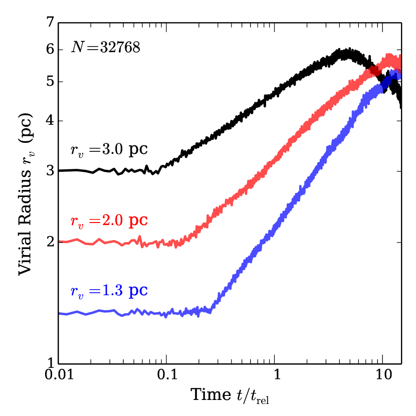
Figure 5: Evolution of the virial radii for three clusters with $N=$32,768. Each curve is labeled by the starting values of the virial radius. In all cases, there is an extended period of power-law expansion, where the expansion is shallowest for the cluster with $r_{v}=3.0$pc. As before, $t_{\rm rel}$ refers to the initial relaxation time.

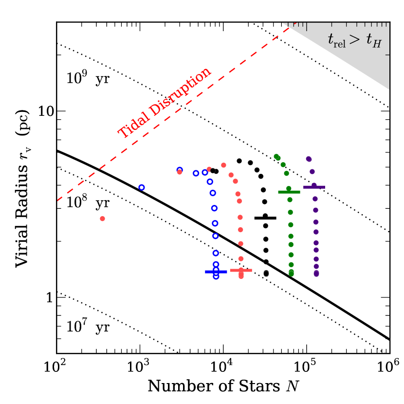
Figure 6: Evolution of five representative clusters in the $r_{v}$-$N$ plane. For each cluster, the horizontal lines marks where the clusters begin sustained binary formation and burning. All clusters start with ${r_{v}=1.3\,}$pc. For the leftmost clusters with an initial $N$ of 32,768 or fewer, we evolve the system until disruption. We evolve the more massive clusters only until $t=15t_{\rm rel}$, before they lose half of their initial cluster members. Note that all curves eventually veer in a direction nearly parallel to, but below, the tidal disruption line.

Whether a cluster’s expansion is powered by central binary heating or pervasive, internal mass loss, the distended system eventually feels the effect of the Galactic tidal field. If the initial virial radius of a cluster exceeds the tidal radius $r_{t}$, as given in equation (6), then that system disrupts in a few crossing times, long before either central binary formation or two-body relaxation can occur. We plot the relation $r_{v}=r_{t}$ as the diagonal, dashed line in Figure 1.

This tidal disruption line represents an extreme limit, as clusters begin to lose members through the Galactic field well before this point is reached. In Figure 6, we show the evolution of five representative clusters that span the collapse line. The virial radius $r_{v}$ plotted is the same as in Figure 1, except that it now represents not the initial value (here 1.3 pc in all cases), but the instantaneous one that evolves with time.

All curves in Figure 6 initially rise upward, signifying expansion at constant $N$. Well before reaching the nominal tidal disruption line, each cluster’s members start to be stripped away, and the curve moves to the left. Thereafter, each cluster follows a path roughly parallel to the tidal line but displaced below it. Thus, the virial radius shrinks with decreasing $N$, but remains a constant fraction (about 0.5) of the current $r_{t}$.

We also mark, with a horizontal bar on each evolutionary curve, the onset of sustained binary formation. From this time forward, there are one or more hard binaries in the system for most time steps of the simulation. In clusters that begin below the collapse line, the first binaries form very quickly because of mass segregation. The event is delayed in systems above the collapse line that eventually undergo core collapse. This delay is caused by the loss of the most massive cluster members through stellar evolution.

Table 1: Characteristic Times of Five Clusters.

$N$	$M_{\rm cl}$	$t_{\rm rel}$	$t_{\rm bin}$	$t_{\rm cc}$	$t_{\rm h}$
	(${\rm M}_{\odot}$)	(Myr)	(Myr)	(Myr)	(Gyr)
8,192	4,800	57	17	—	0.80
16,384	9,600	76	24	—	1.23
32,768	19,000	112	198	—	1.82
65,536	38,000	142	669	923	2.92
131,072	77,000	193	1103	2131	$\cdots$

Key evolutionary times for the five clusters shown in Figure 6, with $r_{v}=1.3\,$pc. The first three columns list the initial population ($N$), mass ($M_{\rm cl}$), and relaxation time ($t_{\rm rel}$). The remaining columns show the times for onset of binary formation ( $t_{\rm bin}$), core collapse ( $t_{\rm cc}$), and tidal stripping of half the initial mass ( $t_{\rm h}$).

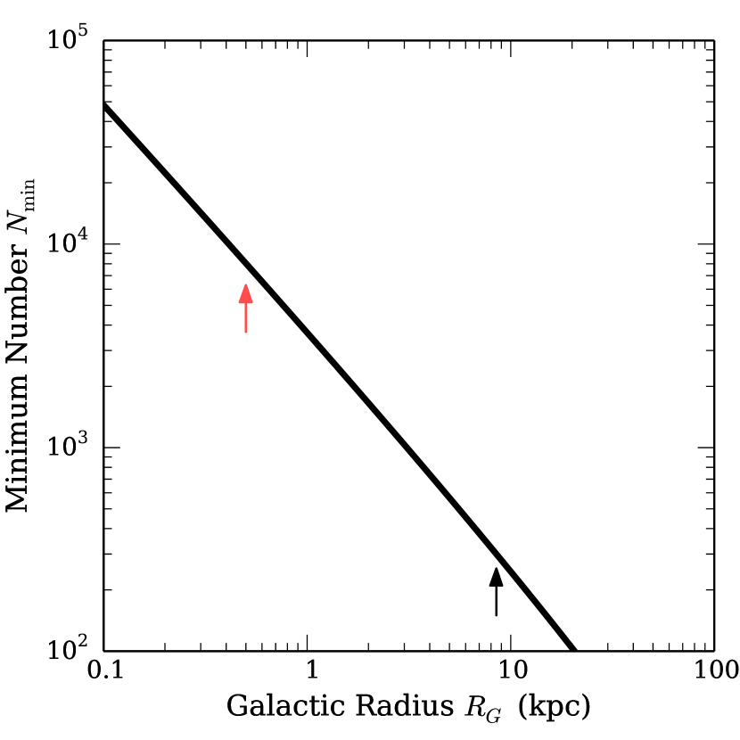
Figure 7: A plot of $N_{\rm min}$, the minimum cluster population capable of undergoing core collapse, shown as a function of the Galactocentric radius $R_{G}$. Most of our simulations were run with $R_{G}=8.5\,$kpc, indicated by the right vertical arrow. To demonstrate the role of $N_{\rm min}$ explicitly, we ran two additional simulations with $R_{G}=0.5\,$kpc, indicated by the left vertical arrow.

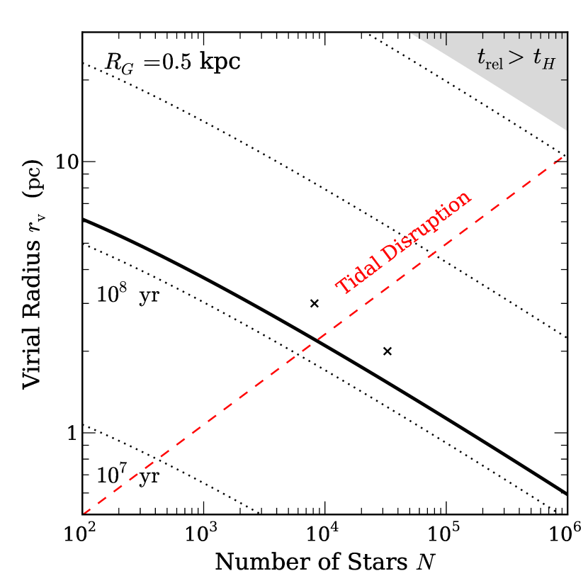
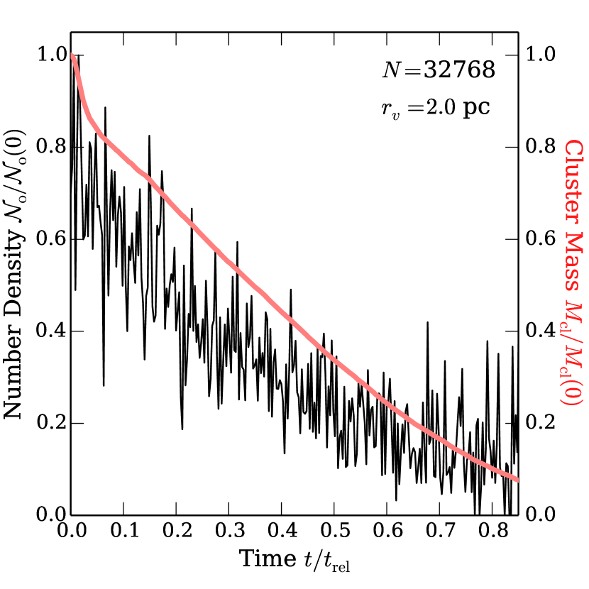
Figure 8: In the left panel, we show the tidal disruption line in the $r_{v}-N$ plane, for $R_{G}=0.5$ kpc. We also indicate the initial conditions and results of our two simulations using this smaller Galactocentric radius. The cluster with $N=$ 8,096 and $r_{v}=3.0$ pc (left cross) disrupts in a few dynamical times. In the right panel, we show (thin black line) the evolution of the central surface density ${\cal N}_{\rm o}$ for a second cluster that is above the collapse line (right cross in the left panel). Its initial conditions place this system close enough to the tidal line that it undergoes global expansion as it disrupts. We also show (thick red line) the decline of the cluster mass $M_{\rm cl}$ due to tidal stripping. We again measure time relative to $t_{\rm rel}$, the initial relaxation time.

In Table 1, we list the characteristic evolutionary times for all five clusters shown in Figure 6. The first three columns give, respectively, the initial population $N$, the total cluster mass, $M_{\rm cl}$, and the relaxation time, $t_{\rm rel}$, where the latter was obtained from equation (1). The time $t_{\rm bin}$ in the fourth column marks the onset of sustained binary formation at the cluster center. For the two clusters starting above the collapse line, we next list $t_{\rm cc}$, the time of core collapse, as judged by the rise in central density (recall eq. 8). Finally, the last column in the table gives $t_{\rm h}$, the time by which the Galactic tide has stripped away half the original mass.

Notice from Table 1 that central binary formation begins before core collapse, if the latter occurs at all. Binaries form in response to the increase in central density, and their heating of the cluster may or may not prevent a further increase in central density. Consider, for example, the cluster with initial $r_{v}=1.3\,$pc and $N=$32,768, which is below the collapse line. As seen in Figure 2, the central density starts to rise at $t\approx 6\,t_{\rm rel}$. Binary heating soon causes the density to fall again. The cluster with the same $r_{v}$, but $N=$131,072, starts above the collapse line. Here, binaries start to form at $t\approx 7t_{\rm rel}$, where Figure 2 shows a relatively small and transient rise in central density. Later in the evolution, binaries continue to form, but their heating is insufficient to halt a second, steeper rise in central density and ultimate core collapse.

Figure 6 shows, as did Figure 1, that the tidal disruption and collapse lines intersect. The cluster population at this intersection, which we denote $N_{\rm min}$, represents the smallest value for which core collapse is possible. That is, clusters starting with $N<N_{\rm min}$ simply expand and then tidally disperse, regardless of their starting virial radii.

To find a quantitative expression for $N_{\rm min}$, we set ${M_{cl}=N_{\rm min}\left<m\right>}$ in equation (6), and then equate $r_{t}$ to the collapse $r_{v}$ in equation (3). We find

$$\frac{N_{\rm min}}{\ln(0.1N_{\rm min})}=8.3\,t_{\rm ms}\frac{m_{*}}{\left<m\right>}\sqrt{\frac{GM_{\rm enc}}{R_{G}^{3}}}.$$ (12)

It is evident that $N_{\rm min}$ depends on the Galactocentric radius $R_{G}$. We show this dependence in Figure 7. Although equation (12) has no simple analytic solution for $N_{\rm min}$, it is well fit by a power law:

$$N_{\rm min}\approx 3500\left(\frac{R_{G}}{1\,{\rm kpc}}\right)^{-9/8}.$$ (13)

Here, we have established the coefficient by using our standard values for $m_{*}$, $\left<m\right>$, and $t_{\rm ms}$, and by assuming an isothermal potential when evaluating $M_{\rm enc}$.

If we set $R_{G}$ equal to the Sun’s Galactocentric radius of 8.5 kpc in equation (13), we obtain $N_{\rm min}=300$, the value seen in Figure 6, and indicated by the right vertical arrow in Figure 7. In order to demonstrate explicitly the significance of $N_{\rm min}$ through simulations, it is infeasible to employ this Solar system value of $R_{G}$, since clusters with $N_{\rm min}\lesssim 300$ are subject to such large-scale fluctuations that their central densities do not evolve smoothly. Accordingly, we have rerun several simulations with $R_{G}$ lowered to 0.5 kpc, where we expect $N_{\rm min}\approx 8000$ (see the left vertical arrow in Fig. 7).

The left panel of Figure 8 shows the new, shifted tidal disruption line in the $r_{v}-N$ plane. Here, $r_{v}$ has its original meaning from Figure 1, i.e., it is the initial virial radius. Also indicated in this panel are the initial conditions for our two simulations, both with $N$ = 32,768. These conditions place both clusters above the collapse line, and yet neither actually undergoes core collapse, as the crosses in the figure indicate.

The cluster starting with $r_{v}=3.0$ pc (left cross in Fig. 8) disrupts within a few dynamical times. When $R_{G}$ was 8.5 kpc, this same system experienced strong core collapse, as seen in the top, middle panel of Figure 2. The cluster with $r_{v}=2.0$ pc also underwent core collapse when $R_{G}$ was 8.5 kpc (middle panel of Fig. 2). With the new $R_{G}$-value, $N\approx 4\,N_{\rm min}$, but the system’s proximity to the tidal line leads to a very different evolution. As seen in the right panel of Figure 8, the central surface density monotonically decreases in less than a relaxation time, as it did when the same cluster was at $R_{G}=8.5\,$kpc (see middle panel of Fig. 2). Now, however, the total cluster mass $M_{\rm cl}$ falls precipitously in that same interval. The combination of tidal stress and internal mass loss promotes global expansion until the system completely disperses. By the last time shown, $t=0.7\,t_{\rm rel}$, the cluster has lost 90 percent of its original population.

5 Discussion

5.1 Summary of results

In this paper, we have shown that a key process in the theoretical account of cluster evolution, internal relaxation leading to core collapse, does not occur for all possible initial conditions. Within the $r_{v}-N$ plane, we have found, first analytically, the collapse line that separates the two distinct evolutionary paths. For this purpose, we compared two time scales. The first is the time required for the most massive stars to settle to the cluster center via dynamical friction. The second is the main-sequence lifetime of these same stars. Clusters for which these two times are equal sit on the collapse line in the $r_{v}-N$ plane.

Only clusters whose initial sizes and populations place them above the collapse line evolve in the manner envisioned by the classical theory, transferring energy outward and eventually undergoing core collapse with a rapid rise in central number density. Those starting below the collapse line globally expand as a result of binary heating that begins before stellar mass loss drives the cluster to expand. The central number density of a cluster born below the collapse line never exceeds its initial value. We have verified, through a suite of numerical simulations, that clusters indeed follow these two paths. In § 5.2 and 5.3 below, we use this theoretical framework, in a preliminary way, to interpret observations of Milky Way clusters.

For the representative sample of clusters in our study, all eventually disrupt tidally, regardless of where they begin in the $r_{v}-N$ plane. Again, we first proceeded analytically, finding a tidal disruption line in the plane. We also tracked the disruption in our simulations, using only the Galactic potential for simplicity. Finally, we have shown that clusters below a certain minimum population reach the point of tidal disruption without ever undergoing core collapse, regardless of their initial size. Near the Sun’s Galactocentric radius, we find that this minimum cluster population is $N_{\rm min}\gtrsim 300$. Future, more detailed simulations that include tidal disruption by spiral arms and giant molecular clouds may increase this figure, although the shape of the tidal line will be similar.

Many of the individual points we have made regarding cluster dynamics have been described previously. It has long been appreciated that introducing a stellar mass spectrum dramatically alters the course of evolution from that of an idealized, uniform-mass system (Aarseth, 1974). Similarly, the critical role of central binaries in both frustrating core collapse and inducing global expansion is well established (Lightman & Shapiro, 1978). That binary heating itself is inoperative for a cluster that is too large and massive is also known (Inagaki, 1984; Heggie & Hut, 2003; Converse & Stahler, 2011), and this fact plays a key role in our evolutionary picture. Furthermore, we have stressed the importance of disentangling the effects of mass segregation from the phenomenon of core collapse.

5.2 Predicting cluster evolution

Our theoretical considerations should be useful for gauging the evolutionary status of real clusters. Drawing the connection is not entirely straightforward, since we do not observe directly any cluster’s initial state or its evolution through time. The salient questions are the following: Given a cluster’s present-day $r_{v}$ and $N$, can we determine which evolutionary path it is on? If the system has not recently undergone core collapse, which should be apparent observationally, will it do so in the future? Or will it evolve instead via global expansion?

Answering these questions is easy for clusters presently located below the collapse line. All such systems will globally expand until they begin to be tidally disrupted. But what about clusters that are currently above the line? For these, we first note that there is another observable, global property of a cluster, its age. This may be determined, in principle, from the distribution of member stars in the HR diagram. It is useful to compare this observed age, $t_{\rm obs}$, with a theoretical “relative age,” $t_{1}$. The latter is the time required for the cluster to reach its present-day $r_{v}$ and $N$ starting from the collapse line. Clusters for which $t_{\rm obs}>t_{1}$ must have started below the collapse line, and thus will globally expand in the future. Here, we are assuming that the cluster is not currently being disrupted. If it is, then its future history is clear but its prior history is uncertain, as we shall discuss.

Our simulations allow us to obtain $t_{1}$ numerically. For a cluster that starts close to the collapse line, $r_{v}$ does not change appreciably until $t\gtrsim 30\,$Myr, at which point stellar mass loss begins to drive expansion. Over the range of $N$ we have explored for clusters near the collapse line, $r_{v}$ then increases as a power law, $r_{v}\propto t^{0.3}$. Using this relation we find

$$t_{1}\approx 30\,\left(\frac{r_{v}}{r_{\rm coll}}\right)^{3.3}{\rm Myr},$$ (14)

where $r_{\rm coll}$ is the virial radius that defines the collapse line in equation (4).

We previously described the global evolution of clusters starting above and below the collapse line. In both cases, there is a similar period of stasis followed by power-law growth (recall Fig. 5). Eventually, however, the cluster radius peaks and then declines as a result of tidal stripping. Clusters starting from different initial conditions can thus traverse the same point in the $r_{v}-N$ plane. For a cluster that is actively being disrupted, the relative time $t_{1}$ is not useful, and the system’s prior history is hard to reconstruct. In some cases, disruption is evident observationally by the presence of tidal streamers (e.g., Odenkirchen et al., 2003). The past history of such systems might be elucidated by studying their internal structure, including the degree of mass segregation.

Table 2: Open Cluster Sample

Name	$N$	$\sigma$	$r_{v}$	Ref
		(km s-1)	(pc)
Hyades	550	0.30	2.5	1
Pleiades (M45)	800	0.36	4.4	2
Praesepe	800	0.67	0.87	3,4
NGC 2168 (M35)	3059	0.65	2.6	5,6
NGC 188	1050	0.41	10.	7,8

Refs: 1. de Bruijne, Hoogerwerf & de Zeeuw (2001), 2. Raboud & Mermilliod (1998), 3. Khalaj & Baumgardt (2013), 4.Madsen, Dravins & Lindegren (2002), 5. Kharchenko et al. (2012), 6.Geller et al. (2010), 7. Platais et al. (2003), 8. Geller et al. (2008)

5.3 Open and globular clusters

Let us now apply these considerations to real systems, starting with open clusters. At present, the number of open clusters with secure values of $r_{v}$ is quite small. The difficulty here is an accurate determination of the mean velocity dispersion $\sigma$, which is easily contaminated by binaries for clusters with intrinsically low dispersions. Table 2 shows the modest result of our own literature search.

In Figure 9, we plot this handful of open clusters in the $r_{v}-N$ plane (squares), as well as a much larger sample of globular clusters (filled circles), to be discussed presently. Here we have not displayed the tidal disruption line. At least one of the open clusters (NGC 188) has a Galactocentric radius quite different from ours, as do most of the globular clusters. In addition, many of the latter lie well outside the Galactic plane, so that our approximate form of the gravitational potential (and thus $r_{t}$) is inappropriate.

Only two open clusters in our current sample lie above the collapse line: the Pleiades and NGC 188. The former is barely over the line, and application of equation (14) yields $t_{1}=40\,$Myr. Since this figure is less than the current age, $t_{\rm obs}=120\,$Myr (Basri, Marcy & Graham, 1996), we conclude that the Pleiades started below the line and will never undergo core collapse. Converse & Stahler (2010) numerically reconstructed the history of this system in detail. They indeed found that it began with a smaller size, $r_{v}\approx 3\,$pc, and is fated to globally expand until the point of tidal disruption.

An open cluster much farther above the collapse line is NGC 188. In this case, we find $t_{1}=800\,$Myr. This number is to be compared with the empirical age of $t_{\rm obs}=6.2\,$Gyr (Meibom et al., 2009), which makes this one of the oldest open clusters in the Galaxy. Since $t_{\rm obs}>t_{1}$, it might appear once more that the cluster began below the collapse line. NGC 188 could have started with $r_{v}=2\,$pc and swelled to its current size in the time $t_{\rm obs}$, assuming its population remained constant. On the other hand, Casetti-Dinescu et al. (2010) detected an associated tidal streamer. If NGC 188 began with a significantly higher $N$ and is now disrupting, then its original location in the $r_{v}-N$ plane is uncertain, as is its fate.

Let us turn finally to globular clusters. The determination of $r_{v}$ is now more straightforward, since the relatively small fraction of binaries cannot appreciably alter the $\sigma$-value observed in the clusters’ spatially unresolved inner regions. In Figure 9, we have placed in the $r_{v}-N$ plane 55 systems whose parameters we obtained from the Harris (1996, Revision 2010) catalog, after assuming a number-to-light ratio of 2. Virtually all the clusters now lie above the collapse line. However, it requires further examination to determine their future evolution.

Suppose we set $t_{1}$ equal to the Hubble time, $t_{H}$. The corresponding line lies parallel to and above the collapse line in the plane. All clusters lying above this line necessarily have $t_{\rm obs}<t_{1}$, and thus will go through core collapse, if they have not done so already. One example is 47 Tuc, an especially large and massive cluster with $r_{v}/r_{\rm coll}=8.9$ and $t_{1}=41\,$Gyr. The latter figure naturally exceeds $t_{\rm obs}=13\,$Gyr (Dotter et al., 2010). A second example, with nearly the same $t_{\rm obs}$-value, is NGC 7078 (M15). Gebhardt et al. (2000) carefully corrected for the cluster’s rotation to obtain $\sigma$, and we use their figure to find $t_{1}=26\,$Gyr. In this case, the system has already undergone core collapse relatively recently (Dull et al., 1997).

Some of the smaller globular clusters that lie closer to the collapse line may have begun below it. Individual systems require study on a case by case basis. There is also a clear need to improve the data on open clusters, so that their evolution can be more fully understood. So too should the origin and fate of massive systems in the Galactic plane, such as Westerlund I (for a review, see Portegies Zwart, McMillan & Gieles, 2010). We leave these tasks to future investigators.

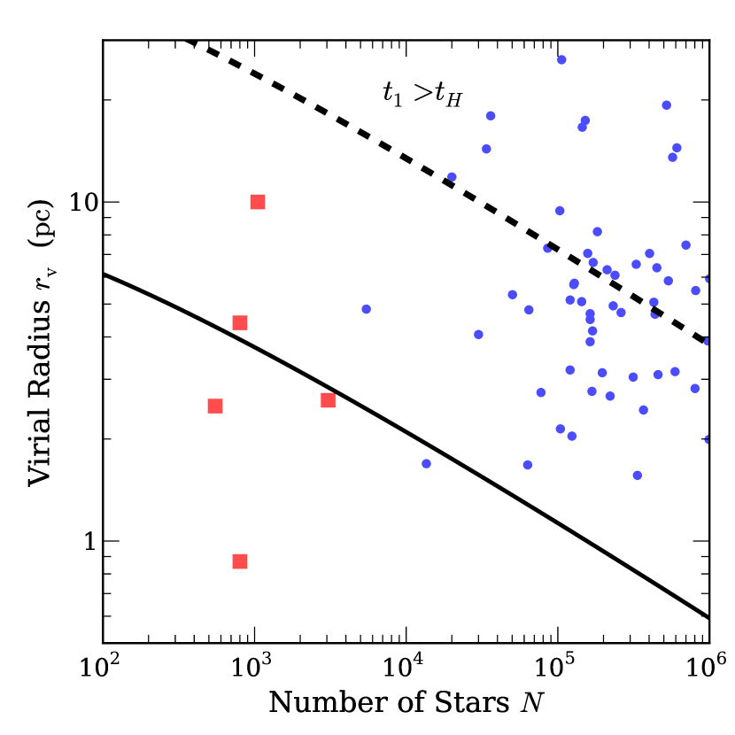
Figure 9: Distribution of observed open clusters (squares) and globular clusters (circles) in the $r_{v}-N$ plane. Data for the open clusters are collected in Table 2. Data for the globular clusters were derived from Harris (1996, Revision 2010). The lower, solid curve is the collapse line. Clusters lying above the upper, dashed curve have $t_{1}$ exceeding the Hubble time $t_{H}$.

References

- Aarseth (1971) Aarseth S. J., 1971, Astrophysics and Space Science, 13, 324
- Aarseth (1974) —, 1974, A&A, 35, 237
- Aarseth (1999) —, 1999, PASP, 111, 1333
- Aarseth, Hénon & Wielen (1974) Aarseth S. J., Hénon M., Wielen R., 1974, A&A, 37, 183
- Basri, Marcy & Graham (1996) Basri G., Marcy G. W., Graham J. R., 1996, ApJ, 458, 600
- Baumgardt & Makino (2003) Baumgardt H., Makino J., 2003, MNRAS, 340, 227
- Bettwieser & Sugimoto (1984) Bettwieser E., Sugimoto D., 1984, MNRAS, 208, 493
- Binney & Tremaine (2008) Binney J., Tremaine S., 2008, Galactic Dynamics: Second Edition. Princeton University Press
- Casertano & Hut (1985) Casertano S., Hut P., 1985, ApJ, 298, 80
- Casetti-Dinescu et al. (2010) Casetti-Dinescu D. I., Girard T. M., Platais I., van Altena W. F., 2010, AJ, 139, 1889
- Cohn (1980) Cohn H., 1980, ApJ, 242, 765
- Converse & Stahler (2010) Converse J. M., Stahler S. W., 2010, MNRAS, 405, 666
- Converse & Stahler (2011) —, 2011, MNRAS, 410, 2787
- de Bruijne, Hoogerwerf & de Zeeuw (2001) de Bruijne J. H. J., Hoogerwerf R., de Zeeuw P. T., 2001, A&A, 367, 111
- Djorgovski & King (1986) Djorgovski S., King I. R., 1986, ApJ, 305, L61
- Dotter et al. (2010) Dotter A. et al., 2010, ApJ, 708, 698
- Dull et al. (1997) Dull J. D., Cohn H. N., Lugger P. M., Murphy B. W., Seitzer P. O., Callanan P. J., Rutten R. G. M., Charles P. A., 1997, ApJ, 481, 267
- Fregeau et al. (2002) Fregeau J. M., Joshi K. J., Portegies Zwart S. F., Rasio F. A., 2002, ApJ, 570, 171
- Gebhardt et al. (2000) Gebhardt K., Pryor C., O’Connell R. D., Williams T. B., Hesser J. E., 2000, AJ, 119, 1268
- Geller et al. (2010) Geller A. M., Mathieu R. D., Braden E. K., Meibom S., Platais I., Dolan C. J., 2010, AJ, 139, 1383
- Geller et al. (2008) Geller A. M., Mathieu R. D., Harris H. C., McClure R. D., 2008, AJ, 135, 2264
- Gieles et al. (2010) Gieles M., Baumgardt H., Heggie D. C., Lamers H. J. G. L. M., 2010, MNRAS, 408, L16
- Giersz & Heggie (1997) Giersz M., Heggie D. C., 1997, MNRAS, 286, 709
- Gnedin, Lee & Ostriker (1999) Gnedin O. Y., Lee H. M., Ostriker J. P., 1999, ApJ, 522, 935
- Goodman (1984) Goodman J., 1984, ApJ, 280, 298
- Gürkan, Freitag & Rasio (2004) Gürkan M. A., Freitag M., Rasio F. A., 2004, ApJ, 604, 632
- Harris (1996) Harris W. E., 1996, AJ, 112, 1487
- Heggie & Hut (2003) Heggie D., Hut P., 2003, The Gravitational Million-Body Problem: A Multidisciplinary Approach to Star Cluster Dynamics
- Hénon (1961) Hénon M., 1961, Annales d’Astrophysique, 24, 369
- Hénon (1965) —, 1965, Annales d’Astrophysique, 28, 62
- Hurley, Pols & Tout (2000) Hurley J. R., Pols O. R., Tout C. A., 2000, MNRAS, 315, 543
- Hurley, Tout & Pols (2002) Hurley J. R., Tout C. A., Pols O. R., 2002, MNRAS, 329, 897
- Inagaki (1984) Inagaki S., 1984, MNRAS, 206, 149
- Ivanova et al. (2005) Ivanova N., Belczynski K., Fregeau J. M., Rasio F. A., 2005, MNRAS, 358, 572
- Khalaj & Baumgardt (2013) Khalaj P., Baumgardt H., 2013, MNRAS, 434, 3236
- Kharchenko et al. (2012) Kharchenko N. V., Piskunov A. E., Schilbach E., Röser S., Scholz R.-D., 2012, A&A, 543, A156
- Kroupa & Weidner (2003) Kroupa P., Weidner C., 2003, ApJ, 598, 1076
- Lamers & Gieles (2006) Lamers H. J. G. L. M., Gieles M., 2006, A&A, 455, L17
- Larson (1970) Larson R. B., 1970, MNRAS, 147, 323
- Lightman & Shapiro (1978) Lightman A. P., Shapiro S. L., 1978, Reviews of Modern Physics, 50, 437
- Lynden-Bell & Wood (1968) Lynden-Bell D., Wood R., 1968, MNRAS, 138, 495
- Madsen, Dravins & Lindegren (2002) Madsen S., Dravins D., Lindegren L., 2002, A&A, 381, 446
- Makino (1996) Makino J., 1996, ApJ, 471, 796
- McMillan, Hut & Makino (1990) McMillan S., Hut P., Makino J., 1990, ApJ, 362, 522
- Meibom et al. (2009) Meibom S. et al., 2009, AJ, 137, 5086
- Meylan & Heggie (1997) Meylan G., Heggie D. C., 1997, The Astronomy and Astrophysics Review, 8, 1
- Miller & Scalo (1979) Miller G. E., Scalo J. M., 1979, ApJS, 41, 513
- Nitadori & Aarseth (2012) Nitadori K., Aarseth S. J., 2012, MNRAS, 424, 545
- Odenkirchen et al. (2003) Odenkirchen M. et al., 2003, AJ, 126, 2385
- Platais et al. (2003) Platais I., Kozhurina-Platais V., Mathieu R. D., Girard T. M., van Altena W. F., 2003, AJ, 126, 2922
- Plummer (1911) Plummer H. C., 1911, MNRAS, 71, 460
- Portegies Zwart, McMillan & Gieles (2010) Portegies Zwart S. F., McMillan S. L. W., Gieles M., 2010, ARAA, 48, 431
- Portegies Zwart, McMillan & Makino (2007) Portegies Zwart S. F., McMillan S. L. W., Makino J., 2007, MNRAS, 374, 95
- Quinlan (1996) Quinlan G. D., 1996, New Astronomy, 1, 255
- Raboud & Mermilliod (1998) Raboud D., Mermilliod J.-C., 1998, A&A, 329, 101
- Röser et al. (2010) Röser S., Kharchenko N. V., Piskunov A. E., Schilbach E., Scholz R.-D., Zinnecker H., 2010, Astronomische Nachrichten, 331, 519
- Sippel et al. (2012) Sippel A. C., Hurley J. R., Madrid J. P., Harris W. E., 2012, MNRAS, 427, 167
- Spitzer (1958) Spitzer, Jr. L., 1958, ApJ, 127, 17
- Spitzer (1969) —, 1969, ApJ, 158, L139
- Tanikawa, Hut & Makino (2012) Tanikawa A., Hut P., Makino J., 2012, New Astronomy, 17, 272
- Trager, King & Djorgovski (1995) Trager S. C., King I. R., Djorgovski S., 1995, AJ, 109, 218
- Trenti, Heggie & Hut (2007) Trenti M., Heggie D. C., Hut P., 2007, MNRAS, 374, 344
- Vesperini, McMillan & Portegies Zwart (2009) Vesperini E., McMillan S. L. W., Portegies Zwart S., 2009, ApJ, 698, 615
- von Hoerner (1960) von Hoerner S., 1960, Zap., 50, 184
- Zonoozi et al. (2011) Zonoozi A. H., Küpper A. H. W., Baumgardt H., Haghi H., Kroupa P., Hilker M., 2011, MNRAS, 411, 1989