On the Casimir Energy of Frequency Dependent Interactions

Abstract

Vacuum polarization (or Casimir) energies can be straightforwardly computed from scattering data for static field configurations whose interactions with the fluctuating field are frequency independent. In effective theories, however, such interactions are typically frequency dependent. As a consequence, the relationship between scattering data and the Green’s function is modified, which may or may not induce additional contributions to the vacuum polarization energy. We discuss several examples that naturally include frequency dependent interactions: (i) scalar electrodynamics with a static background potential, (ii) an effective theory that emerges from integrating out a heavy degree of freedom, and (iii) quantum electrodynamics coupled to a frequency dependent dielectric material. In the latter case, we argue that introducing dissipation as required by the Kramers–Kronig relations requires the consideration of the Casimir energy within a statistical mechanics formalism, while in the absence of dissipation we can work entirely within field theory, using an alternative formulation of the energy density.

I Introduction

Vacuum polarization (or Casimir) energies arise when quantum fluctuations interact with localized) background fields such as solitons. These interactions change the zero–point energies of the fluctuations. Summing these changes gives a non–trivial contribution to the energy at order $\hbar$, or in the language of Feynman diagrams, at one loop. As is common for loop diagrams, ultra–violet divergences occur in this calculation. It is essential that these divergences are unambiguously canceled by fixed counterterms whose coefficients do not depend on the specification of the background. In the case of static backgrounds whose interactions with quantum fields do not involve the conjugate momenta of these fields, spectral methods are well known to accomplish this task Graham et al. (2009). This formalism is well founded in quantum field theory Graham et al. (2002). For completeness we will provide a more heuristic derivation in this introduction, based on techniques from quantum mechanics, and review the essentials of the quantum field theory derivation in section II. The main goal of this paper, however, is to explore the spectral method in cases where the interaction is frequency dependent, and to discuss the possible modifications necessary to handle such cases.

As mentioned earlier, it is necessary to sum the changes in the zero–point energies due to the interaction with the background. There are two types of energy eigenstates that lead to zero point energies, (i) bound states with discrete eigenvalues $\omega_{n}$ and (ii) continuum states with the dispersion relation $\omega=\frac{k^{2}}{2m}$ or $\omega^{2}=k^{2}+m^{2}$ for non–relativistic and relativistic theories, respectively. Here $k$ is the asymptotic wave–number of the quantum fluctuation and $m$ is its mass. Since there are no bound states (b.s.) without the background, the bound states contribute just $\frac{1}{2}\sum_{n={\rm b.s.}}\,|\omega_{n}|$ to the vacuum polarization energy. The continuum piece is often expressed as an integral over the frequency weighted by the change of the density of states, $\Delta\rho(k)$, caused by the interaction. In order to find $\Delta\rho(k)$, boundary conditions far away from the interaction regime are imposed to discretize and count the states. Eventually this boundary is sent to infinity. Far away from the interaction regime, however, all information about the background is encoded in the phase shift $\delta(k)$ that the interaction imprints on the quantum fluctuation. A typical boundary condition is then of the form ${\rm sin}(kL+\delta(k))=0$, where $L$ refers to the position of the boundary. Counting the states is then as simple are demanding that $kL+\delta(k)=n(k)\pi$. The density of states is the derivative $\partial n(k)/\partial k$ giving $\pi\,\Delta\rho(k)=\partial\delta(k)/\partial k$ as $L\to\infty$. This relation between the scattering phase shift and the density of states is also known as the Krein–Friedel–Lloyd formula; see Ref. Faulkner (1977) and references therein. Putting these results together yields the phase shift formula for the computation of vacuum polarization energies

$$E_{\rm vac} = \int\frac{dk}{2\pi}\sqrt{k^{2}+m^{2}}\,\frac{\partial}{\partial k}\delta(k)+\frac{1}{2}\sum_{n={\rm b.s.}}\,|\omega_{n}|+E_{\rm c.t.}$$ (1)

$$= \int\frac{dk}{2\pi}\sqrt{k^{2}+m^{2}}\,\left[\frac{\partial}{\partial k}\delta(k)\right]_{N}+\frac{1}{2}\sum_{n={\rm b.s.}}\,|\omega_{n}|+E_{\rm FD}^{(N)}+E_{\rm c.t.}\,,$$ (3)

which also includes the counterterm (c.t.) contribution. In the second equation we have indicated the subtraction of the first $N$ terms of the Born series from the phase shift. The Born series orders scattering data according to increasing powers of the background interaction and may be constructed by iterating the wave–equation. The same expansion can be alternatively formulated in terms of Feynman diagrams, and $E_{\rm FD}$ in Eq. (3) adds back in exactly what the Born terms subtracted. If $N$ is large enough the momentum integral will be finite, and the sum $E_{\rm FD}^{(N)}+E_{\rm c.t.}$ can be regularized and renormalized by standard techniques from perturbative field theory. We stress that the Born and Feynman expansions have solely been introduced to identify and eventually cancel the ultra–violet divergences. This does not imply that these series are good approximations to the (one–loop) vacuum polarization energy; they might, in fact, not even converge. The spectral method sketched above has proven to be a very versatile tool to compute vacuum energies in sufficiently symmetric static backgrounds. It has been extended successfully to a wide range of situations, from cosmic strings Graham et al. (2011) over soliton stabilization Farhi et al. (2000) to interfaces and extra dimensions Graham et al. (2001). The Krein–Friedel–Lloyd formula has been the basis of many studies of quantum corrections to classical soliton energies; see for example one dimensional models in Refs.Dashen et al. (1974); Gervais et al. (1975); Cahill et al. (1976); Nakahara and Maki (1982); Graham and Jaffe (1999); Flores-Hidalgo (2002) or the three dimensional Skyrme model in Refs.Moussallam and Kalafatis (1991); Meier and Walliser (1997); Weigel (2008).

The above heuristic derivation shows that in order to find the density of states and thus the vacuum polarization energy, we must compare modes with different (albeit infinitesimally close) frequencies. Thus it is not at all obvious that the above argument for the density of states carries through when the interaction with the background becomes frequency dependent. This question arises irrespective of whether or not the field equations are diagonal in the frequency. Furthermore we have assumed that each mode contributes exactly ${\textstyle\frac{1}{2}}\omega$. Effective action arguments suggest that this assumption essentially boils down to the statement that even with the frequency dependent interaction included the energy of the static background is still the negative of its Lagrange function. This statement can undergoes modifications when the interaction involves a time derivative of the quantum field. Here we will consider a variety of models with frequency dependent interactions and study whether and under what conditions the above simple description for the vacuum energy can be maintained.

In the next section we review the quantum field theory derivation of Eq. (3) for static interactions. Subsequently we investigate the modifications necessary for a number of examples with frequency dependent interactions. The simplest model that leads to a frequency dependent interaction is the gauge invariant coupling of a scalar field to a static electromagnetic background. In section III we study this example and find that computing its vacuum polarization energy does not require any approximation and, furthermore, that Eq. (3) holds without modification.

Frequency dependent interactions also emerge in effective theories that result from integrating out some of the degrees of freedom. Such a scenario is often encountered in particle physics. Typically, a local energy density and a scattering problem can only be formulated in the effective theory once certain approximations are performed. But even with such approximations, frequency dependence must be retained to account for renormalizability. In the specific example of section IV we will see that Eq. (3) is also valid without modifications. However, it is essential to consistently approximate both the wave–equations and the energy density when constructing the effective theory.

In both examples we will observe that indeed significant changes to the energy density and the scattering data occur when frequency dependent interaction are involved. These changes tend to cancel, so that Eq. (3) remains correct in such cases. However, the necessary cancellations of non–standard contributions involving the background potential are very delicate, and it is by no means obvious that the use of Eq. (3) without modifications will succeed in all cases. In section V we will study the important problem of electrodynamics in a dielectric. For the Casimir problem to remain under control in the ultraviolet, we must have a frequency–dependent dielectric function. In order to obey the Kramers-Kronig relations, such a dielectric must include dissipation, which in the Casimir problem represents a coupling of electromagnetic fluctuations to fluctuations in the microscopic matter degrees of freedom. Refs. Rahi et al. (2009); Kenneth and Klich (2006, 2008) formulate the Casimir energy in this case as an ensemble average in statistical mechanics. In this approach the standard expression for the energy in a dielectric is identified from a calculation of the free energy. When translated intro scattering theory, it induces extra terms in Eq. (3). These terms can play an important role in determining the sign of the Casimir self–stress Graham et al. (2013). Alternatively, one can consider a dielectric without dissipation, in which case the problem can be formulated within field theory, at the cost of violation of the Kramers–Kronig relations. In this case, one obtains a different expression for the (now conserved) energy, one that has been obtained previously in classical electromagnetism as an approximation at frequencies where dissipation is negligible Landau and Lifshitz (1986), and that has also been discussed in the context of Casimir calculations Brevik and Milton (2008); Milton et al. (2010); Rosa et al. (2010, 2011). Notably, this form of the energy has the effect of exactly canceling the extra terms appearing in Eq. (3). We summarize our conclusions in section VI, and in an appendix we comment on the construction of a conserved energy from a wave–equation with an arbitrary frequency dependence.

II Review of the Spectral Method

We start with a brief review of how the phase shift formula (3) for the vacuum polarization energy can be derived in the case that the interaction is frequency independent. For simplicity, we only consider the anti-symmetric channel in $d=1$ space dimensions, which can also be used to describe $S$-wave scattering in $d=3$. For further details of this computation and the generalization to higher dimensions and angular momenta, the reader is referred to appendix A of Ref. Graham et al. (2002). For a relativistic boson of mass $m$, the scattering of a fluctuation mode with frequency $\omega$ and momentum $k$ (related by $\omega=\sqrt{k^{2}+m^{2}}$) off a static background $V(x)$ is described by the wave–equation

$$\left[-\partial_{x}^{2}+V(x)\right]\psi_{k}(x)=k^{2}\psi(x)$$ (4)

from which the Green’s function can be obtained as

$$G(x,x^{\prime},k)=\frac{\phi_{k}(x_{<})f_{k}(x_{>})}{F(k)}\,.$$ (5)

Here $\phi_{k}(x)$ and $f_{k}(x)$ are the regular and Jost solutions to the wave–equation (4) that are defined by suitable boundary conditions at $x=0$ and $x\to\infty$, respectively Newton (1982); Chadan and Sabatier (1977). The denominator contains the Jost function $F(k)\sim\lim_{x\to 0}f_{k}(x)$ whose negative phase is the scattering phase shift $\delta(k)$. By construction, $F(k)$ has simple zeros at $k=i\kappa_{n}$, where $\kappa_{n}$ are the bound state wave–numbers. From the wave–equation (4) we also find the Wronskian

$$W\left[f_{k}(R),\phi_{q}(R)\right]=F(k)+(k^{2}-q^{2})\int_{0}^{R}dx\,f_{k}(x)\phi_{q}(x)\,,$$ (6)

for wave–functions with different momenta. Obviously, this relation must be modified once the frequency dependence on the right hand side of Eq. (4) is altered. For the moment, we adhere to Eq. (6) and differentiate with respect to $k$, take the limit $q\to k$, and divide by $F(k)$ to obtain an equation for the Green’s function at coincident points

$$W\left[\frac{\partial f_{k}(R)}{\partial k},\phi_{q}(R)\right]=\frac{\partial}{\partial k}\,{\rm ln}\left[F(k)\right]+2k\int_{0}^{R}dx\,G(x,x,k)\,.$$ (7)

After subtracting the non–interacting ($V\equiv 0$) analog of this formula and taking the limit $R\to\infty$, the left hand side vanishes Graham et al. (2002). As a consequence,

$$0=\frac{\partial}{\partial k}\,{\rm ln}\left|F(k)\right|-i\frac{\partial}{\partial k}\delta(k)+2k\int_{0}^{\infty}dx\,\left[G(x,x,k)-G^{(0)}(x,x,k)\right]\,.$$ (8)

The vacuum energy density in such simple systems may be expressed as

$$u(x)=\int\frac{dk}{\pi}\sqrt{k^{2}+m^{2}}\,k\,\mathsf{Im}\left[G(x,x,k)-G^{(0)}(x,x,k)\right]+\sum_{n={\rm b.s.}}\frac{|\omega_{n}|}{2}|\psi_{n}(x)|^{2}+\ldots\,,$$ (9)

since the poles in the imaginary part of the Green’s function determine the density of scattering states. The discrete sum runs over the bound state solutions to the wave–equation (4) and the ellipsis denotes total derivative terms and counterterm contributions. Integrating the spatial coordinate and taking the imaginary part of Eq. (8) yields the vacuum energy

$$E_{\rm vac}=\int_{0}^{\infty}dx\,u(x)=\int\frac{dk}{2\pi}\sqrt{k^{2}+m^{2}}\,\frac{\partial}{\partial k}\delta(k)+\frac{1}{2}\sum_{n={\rm b.s.}}\,|\omega_{n}|\,$$ (10)

up to renormalization. This is the phase shift formula relating the vacuum polarization energy of the background field configuration to the phase shift for quantum mechanical scattering off that background. The step between Eqs. (6) and (7) in this derivation shows that we should expect modifications to that formula must be expected when there is a more complicated frequency dependence in the wave–equation.

In the above we have followed the standard line of argument that is based on relating the (local) density of states to the imaginary part of the Green’s function at coincident points. Next we show that Eq. (10) can also be obtained from arguments based entirely on scattering data. This approach is advantageous because the construction of a Green’s function may be difficult for frequency dependent problems, since we may not have an underlying completeness relation for the scattering solutions. Instead, we only assume that the frequency dependence of the interaction does not create any (further) singularities in the upper half plane of complex momenta. The energy density will involve $\mathsf{Im}\,\Gamma(x,x,k)$ with

$$\Gamma(x,y,k)=\int_{0}^{\infty}\frac{dq}{2\pi}\frac{\psi^{\ast}_{q}(x)\psi_{q}(y)}{(k+i\epsilon)^{2}-q^{2}}+\mbox{bound state contribution}$$ (11)

where

$$\psi_{q}(x)=\frac{q}{F(q)}\,\phi_{q}(x)=\frac{2i}{F(q)}\left[F(q)f_{-q}(x)-F(-q)f_{q}(x)\right]$$ (12)

is the physical scattering solution. We need to show that $\Gamma(x,y,k)$ equals the right hand side of Eq. (5). For small arguments the real regular solution is well defined, as is the Jost solution for large arguments. Thus a suitable parameterization of the product of the scattering solutions is ($F^{\ast}(q)=F(-q)$ for real $q$)

$$\psi^{\ast}_{q}(x)\psi_{q}(y)=\frac{2iq}{F(q)F(-q)}\phi_{q}(x)\left[F(q)f_{-q}(y)-F(-q)f_{q}(y)\right]$$ (13)

in the case that $x=r_{<}$ and $y=r_{>}$. Since $\phi_{q}(x)=\phi_{-q}(x)$ we can extend the $q$–integral in Eq. (11) to cover the entire real axis by changing $q\to-q$ in the first term on the right hand side of Eq. (13)

$$\Gamma(x,y,k)=2i\int_{-\infty}^{\infty}\frac{dq}{2\pi}\,\frac{q}{F(q)}\frac{\phi_{q}(r_{<})f_{q}(r_{>})}{(k+i\epsilon)^{2}-q^{2}}+\mbox{bound state contribution}\,.$$ (14)

With the assumption that no additional singularities emerge from the frequency dependent interaction, the poles at $q=k+i\epsilon$ will directly yield the right hand side of Eq. (5). The poles due to the roots of the Jost function will compensate for the bound state contribution, and the roots at $q=-(k+i\epsilon)$ do not contribute because we close the contour integral in the upper half of the complex $q$–plane. Thus $\Gamma(x,x^{\prime},k)$ equals the right hand side of Eq. (5) and the derivation of the phase shift formula can be completed without requiring that $\Gamma$ is a Green’s function.

III Scalar Electrodynamics

Scalar electrodynamics with a static electric potential produces a frequency dependent background for the scalar quantum fluctuations. The simplest case is in $d=1$ spatial dimension so that the gauge field is $A^{\mu}=(V(x),0)$, which also satisfies the Lorentz condition $\partial_{\mu}A^{\mu}=0$. The case $d=1$ also has the advantage that all divergences cancel in a gauge invariant regularization, but otherwise the number of space dimensions is irrelevant for the present study. The Lagrangian for a scalar field $\Phi$ with mass $M$ coupled to an electromagnetic background field is

$$\mathcal{L}=\left(D_{\mu}\Phi\right)^{\ast}\left(D^{\mu}\Phi\right)-M^{2}\Phi^{\ast}\Phi\qquad{\rm with}\qquad D_{\mu}=\partial_{\mu}+iA_{\mu}\,,$$ (15)

which implies the effective action of the photon field $A_{\mu}$,

$$S[A_{\mu}]=i\,{\rm Tr}\,{\rm log}\left[\partial^{2}+M^{2}-i\overleftarrow{\partial}_{\mu}A^{\mu}+iA_{\mu}\partial^{\mu}-A_{\mu}A^{\mu}\right]=i\,{\rm Tr}\,{\rm log}\left[\partial^{2}+M^{2}-i\overleftarrow{\partial}_{t}V+iV\partial_{t}-V^{2}\right]\,.$$ (16)

Here and in the following, the arrow denotes the direction of differentiation. The symbol ${\rm Tr}$ describes a functional trace that also includes space–time integration. Of course, this functional trace is superficially divergent at large momenta, and we implicitly assume some gauge invariant regularization, such as dimensional regularization.

As a first step, we want to use functional methods to establish a relationship between the action in Eq. (16) and the quantum (or vacuum polarization) energy. To do so we start from the energy density operator

$$T^{00}(x)=\frac{\partial\mathcal{L}}{\partial\dot{\Phi}}\dot{\Phi}+\frac{\partial\mathcal{L}}{\partial\dot{\Phi}^{\ast}}\dot{\Phi}^{\ast}-\mathcal{L}=\Phi^{\ast}\left(\overleftarrow{\partial}_{t}\overrightarrow{\partial}_{t}+\overleftarrow{\partial}_{x}\cdot\overrightarrow{\partial}_{x}+M^{2}-V^{2}\right)\Phi\,.$$ (17)

The corresponding quantum energy density becomes

$$\langle T^{00}(x)\rangle=-i\,{\rm Tr}\,\Big{[}\left(\partial^{2}+m^{2}-i\overleftarrow{\partial}_{t}V+iV\partial_{t}-A_{\mu}A^{\mu}\right)^{-1}\delta^{(2)}(x-x_{\rm op})\left(\overleftarrow{\partial}_{t}\overrightarrow{\partial}_{t}+\overleftarrow{\partial}_{x}\cdot\overrightarrow{\partial}_{x}+M^{2}-V^{2}\right)\Big{]}\,.$$ (18)

Notice that $x_{\rm op}$ denotes the position operator, while $x$ is the argument of the density on the left hand side. This expression simplifies because the potential is static, $V=V(x)$, so that the temporal part of the functional trace can be written as a single frequency integral. Furthermore the vacuum polarization energy is obtained by integration over all space, which removes the $\delta$–function completely,

$$E_{\rm vac}=-i\int\frac{d\omega}{2\pi}\,{\rm Tr}^{\prime}\,\Big{[}\left(-\omega^{2}-\partial_{x}^{2}+M^{2}-2\omega V-V^{2}\right)^{-1}\left(\omega^{2}+\overleftarrow{\partial}_{x}\cdot\overrightarrow{\partial}_{x}+M^{2}-V^{2}\right)\Big{]}\,,$$ (19)

The functional trace ${\rm Tr}^{\prime}$ no longer includes the integral over the time variable. Note that the vacuum energy $E_{\rm vac}$ still contains the contribution from the free case ($A_{\mu}\equiv 0$), while the Casimir energy $E_{\rm cas}=E_{\rm vac}-E_{\rm vac}^{(0)}$ is the change in the vacuum energy due to the photon background. We can now integrate the spatial derivatives by parts and assume that the boundary terms vanish either because the space interval is infinite and the fields drop off sufficiently fast, or because the Boson fields obey periodic boundary conditions in a finite space interval. We obtain

$$E_{\rm vac} = =i\int\frac{d\omega}{2\pi}\,\omega\,{\rm Tr}^{\prime}\,\Big{[}\left(-\omega^{2}-\partial_{x}^{2}+M^{2}-2\omega V-V^{2}\right)^{-1}\frac{\partial}{\partial\omega}\left(-\omega^{2}-\partial_{x}^{2}+m^{2}-2\omega V-V^{2}\right)\Big{]}+c_{1}$$ (20)

$$= i\int\frac{d\omega}{2\pi}\,\omega\,\frac{\partial}{\partial\omega}{\rm Tr}^{\prime}\,{\rm log}\Big{[}-\omega^{2}-\partial_{x}^{2}+M^{2}-2\omega V-V^{2}\Big{]}+c_{2}$$ (22)

where the constants $c_{1}$ and $c_{2}$ are independent of the background potential $V$ (though they may require regularization). Comparison with Eq. (16) immediately shows that

$$E_{\rm vac}=-\frac{1}{T}S[A_{\mu}]\,,$$ (23)

where the (infinitely large) time interval $T$ entered by restoring the full functional trace. The last equation is of course well known Weinberg (1995), but still a bit surprising in the present context, since the Hamiltonian derived from Eq. (15) still contains time derivatives and the problem is thus not completely static, even though $V(x)$ depends only on the space variable. The additional time derivatives in the interaction complicate the Legendre transformation between energy and action per unit time, but Eq. (23) still holds in this case.

The canonical approach is also unconventional but straightforward; it can be formulated as an application of the random phase approximation Ring and Schuck (1980). After Fourier transforming the time-dependence, the field equations turn into wave-equations for bound states $\phi_{n}(x)$ with discrete energies $|\omega_{n}|<M$, and for scattering solutions $\phi_{k}^{(\pm)}(x)$ with energies $\pm\omega_{k}$ (where $\omega_{k}=\sqrt{k^{2}+M^{2}}>0$),

$$\Big{[}-\partial_{x}^{2}-V(x)^{2}+2\omega_{n}\,V(x)+M^{2}\Big{]}\,\phi_{n}(x) = \omega_{n}^{2}\,\phi_{n}(x)$$ (24)

$$\Big{[}-\partial_{x}^{2}-V(x)^{2}\pm 2\omega_{k}\,V(x)+M^{2}\Big{]}\,\phi_{k}^{(\pm)}(x) = \omega_{k}^{2}\,\phi_{k}^{(\pm)}(x)\,.$$ (25)

Since the theory is not CP-invariant, the existence of a bound state with energy $\omega_{n}$ does not imply the existence of a corresponding bound state with negative energy $(-\omega_{n})$, and likewise $\phi_{k}^{(+)}(x)\neq\phi_{k}^{(-)}(x)$ for the scattering states.

To determine the normalization of these states, let us first consider the bound state equation (24). Multiplying this equation by $\phi_{m}(x)$ from the right, integrating over space and subtracting the same equation with the replacement $m\leftrightarrow n$ immediately shows

$$(\omega_{m}-\omega_{n})\int dx\,\phi_{m}(x)\left[\omega_{m}+\omega_{n}-2V(x)\right]\,\phi_{n}(x)\,=0\,.$$ (26)

The norm of the bound state wave functions can thus be determined by the orthogonality relation

$$\int dx\,\phi_{m}(x)\big{[}\omega_{m}+\omega_{n}-2V(x)\big{]}\phi_{n}(x)=\delta_{mn}\,{\rm sgn}(\omega_{m})\,.$$ (27)

A similar consideration for the scattering states leads to

$$\int dx\,\phi_{k}^{(s)}(x)\big{[}s\omega_{k}+r\omega_{q}-2V(x)\big{]}\phi_{q}^{(r)}(x)=2\pi s\delta_{sr}\,\delta(k-q)\,.$$ (28)

Of course, bound state and continuum solutions are orthogonal

$$\int dx\,\phi_{k}^{(s)}(x)\big{[}s\omega_{k}+\omega_{n}-2V(x)\big{]}\phi_{n}(x)=0\,.$$ (29)

With these orthonormality conditions (and the corresponding completeness relations, cf. Eq. (36) below), we can decompose the field operator in the usual fashion,

$$\Phi(x,t)=\sum_{\omega_{n}\geq 0}\,a_{n}\,\phi_{n}(x){\rm e}^{-i\omega_{n}t}+\sum_{\omega_{n}<0}b_{n}^{\dagger}\phi_{n}(x){\rm e}^{-i\omega_{n}t}+\int_{0}^{\infty}\frac{dk}{2\pi}\left[a(k)\phi_{k}^{(+)}(x){\rm e}^{-i\omega_{k}t}+b^{\dagger}(k)\phi_{k}^{(-)}(x){\rm e}^{i\omega_{k}t}\right]\,.$$ (30)

To quantize the model, we have to impose the canonical equal time commutation relations between the field $\Phi$ and its conjugate momentum $\Pi$, which involves a covariant rather than an ordinary time derivative,

$$\Pi(x,t)=\frac{\partial\mathcal{L}}{\partial\dot{\Phi}(x,t)}=\dot{\Phi}^{\ast}(x,t)-iV(x)\Phi^{\ast}(x,t)\,.$$ (31)

Inserting the decomposition Eq. (30) in these commutation relations, and using the orthogonality conditions, Eqs. (27)–(29) to extract the expansion coefficients, we obtain the usual ladder algebra

$$\left[a_{n},a_{m}^{\dagger}\right] =\delta_{nm}\,, \left[b_{n},b_{m}^{\dagger}\right] =\delta_{nm}$$

$$\left[a(k),a^{\dagger}(q)\right] =2\pi\delta(k-q)\,, \qquad\qquad\left[b(k),b^{\dagger}(q)\right] =2\pi\delta(k-q)$$ (32)

where all other combinations vanish. We use these creation and annihilation operators to construct a Fock space and compute the vacuum matrix element of the energy density operator

$$2T^{00}(x)=\dot{\Phi}^{\ast}\dot{\Phi}^{\dagger}-\Phi^{\ast}\left(\partial_{t}^{2}+2iV\partial_{t}\right)\Phi^{\dagger}+\dot{\Phi}\dot{\Phi}^{\dagger}-\Phi\left(\partial_{t}^{2}-2iV\partial_{t}\right)\Phi^{\dagger}+\ldots\,,$$ (33)

where the ellipsis refers to total space derivatives that do not contribute to the integrated energy. We obtain by textbook techniques

$$\big{\langle}\,0\,\big{|}\,T^{00}(x)\,\big{|}\,0\,\big{\rangle}=\sum_{n}\omega_{n}\,\phi_{n}(x)\big{[}\omega_{n}-V(x)\big{]}\phi_{n}(x)+\sum_{s=\pm}\int_{0}^{\infty}\frac{dk}{2\pi}\,\omega_{k}\,\phi_{k}^{(s)}(x)\,\big{[}\omega_{k}-s\,V(x)\big{]}\,\phi_{k}^{(s)}(x)+\ldots\,.$$ (34)

At this point, we see that the vacuum energy density indeed contains a non-standard factor which involves the interaction explicitly. However, the same factor appears in Eqs. (27) and (28). When this is taken into account, the total vacuum energy becomes

$$E_{\rm vac}=\int dx\,\big{\langle}\,0\,\big{|}\,T^{00}(x)\,\big{|}\,0\,\big{\rangle}=\frac{1}{2}\sum_{n}|\omega_{n}|+\frac{L}{2}\int_{0}^{\infty}\frac{dk}{2\pi}\,\left(2\omega_{k}\right)\,,$$ (35)

where $L=2\pi\delta(0)$ is the spatial volume (length) of the universe. This is precisely the usual sum over zero point energies. Of course, this expression is highly divergent and only formal at this point. (We will eventually have to subtract the non–interacting case $V=0$, and add appropriate counterterms in higher dimensions.) The important conclusion is, however, that the frequency dependence in the interaction does not alter the expression for the vacuum energy in the present case.

Let us next study how the spectral method applies in this model. We first note the completeness relations for the scattering and bound states that are compatible with Eqs. (27) and (28),

$$\sum_{n}|\omega_{n}|\,\phi_{n}(x)\,\phi_{n}(y) +\int_{0}^{\infty}\frac{dk}{2\pi}\,\sum_{s=\pm}\,\omega_{k}\,\phi_{k}^{(s)}(x)\,\phi_{k}^{(s)}(y) \,\,=\,\, \delta(x-y)$$

$$\sum_{n}\mathrm{sgn}(\omega_{n})\,\phi_{n}(x)\,\phi_{n}(y) +\int_{0}^{\infty}\frac{dk}{2\pi}\,\sum_{s=\pm}\,s\,\phi_{k}^{(s)}(x)\,\phi_{k}^{(s)}(y) \,\,=\,\, 0\,.$$ (36)

The second relation would be a trivial identity in a CP–invariant model, but here it follows as a consistency condition on Eqs. (27) and (28). We separate the Green’s function in frequency space ($|\omega|\geq M$) in three pieces, viz. the bound state part plus the negative and positive frequency contributions from the continuum

$$G(x,y,\omega) =G^{\rm(b.s.)}(x,y,\omega)+\Theta(\omega)G^{(+)}(x,y,k)+\Theta(-\omega)G^{(-)}(x,y,k)$$

$$G^{\rm(b.s.)}(x,y,\omega) =\sum_{n}{\rm sgn}(\omega_{n})(\omega_{n}+\omega)\frac{\phi_{n}(x)\phi_{n}(y)}{\omega_{n}^{2}-\omega^{2}}$$

$$G^{(\pm)}(x,y,k) =\sum_{s=\pm}\int_{0}^{\infty}\frac{dq}{2\pi}\left(\omega_{q}\pm s\omega_{k}\right)\frac{\phi_{q}^{(s)}(x)\phi_{q}^{(s)}(y)}{q^{2}-(k+i\epsilon)^{2}}\,,$$ (37)

where $k\equiv\sqrt{\omega^{2}-M^{2}}>0$. Because of the completeness relations (36), this Green’s function obeys

$$\left[\omega^{2}-2\omega V(x)+\partial_{x}^{2}+V^{2}(x)-M^{2}\right]G(x,y,\omega)=-\delta(x-y)\,.$$ (38)

The boundary conditions on the Green’s function (the $i\epsilon$ prescription) were chosen such that the poles for $\mathsf{Im}(k)>0$ are those of the bound state wave numbers, i.e. $G$ has the same analytic structure as in ordinary scattering theory, cf. Eq. (5).

Since the square of the bound state wave functions is real in our normalization, only the continuum contribution to the Green’s function can have an imaginary part, which stems from $\mathsf{Im}[q^{2}-(k+i\epsilon)^{2}]^{-1}=\pi\delta(q^{2}-k^{2})$. It is then straightforward to show from Eq. (34) that the vacuum energy density is

$$u(x)=\sum_{n}\omega_{n}\phi_{n}(x)\big{[}\omega_{n}-V(x)\big{]}\phi_{n}(x)+\frac{1}{\pi}\int_{-\infty}^{\infty}d\omega\,\omega\big{[}\omega-V(x)\big{]}\,\mathsf{Im}\left[G(x,x,\omega)-G^{(0)}(x,x,\omega)\right]\,.$$ (39)

This is the analog of Eq. (9) in the standard spectral method. It should be stressed again that the modified normalization of states leads to non-standard coefficients that involve the background potential explicitly.

The last step is to relate the vacuum energy to scattering data. To do so, we find the analog of Eq. (6) from the wave–equation (24)

$$W\left[f^{(s)}_{k}(R),\phi^{(s)}_{q}(R)\right]=F^{(s)}(k)+\int_{0}^{R}dx\left[\omega_{k}^{2}-\omega_{q}^{2}-2s(\omega_{k}-\omega_{q})V(x)\right]f^{(s)}_{k}(x)\phi^{(s)}_{q}(x)\,,$$ (40)

where the superscript $s=\pm 1$ on the scattering wave functions denotes the positive and negative frequency channels. Retracing the steps that in the standard approach led to Eq. (8), we find,

$$0=\sum_{s=\pm}\left\{\frac{\partial}{\partial k}\,{\rm ln}\left|F^{(s)}(k)\right|-i\frac{\partial}{\partial k}\delta^{(s)}(k)\right\}+2\,\frac{k}{\omega_{k}}\int_{0}^{\infty}dx\,\left[\omega_{k}-V(x)\right]\left[G(x,x,\omega_{k})-G^{(0)}(x,x,\omega_{k})\right]\,,$$ (41)

after summation over both frequency channels. Taking the imaginary part and comparing with the spatial integral of Eq. (39), we obtain

$$E_{\rm vac}=\int_{0}^{\infty}dx\,u(x)=\frac{1}{2}\sum_{n}\,|\omega_{n}|+\int_{0}^{\infty}\frac{dk}{2\pi}\,\omega_{k}\frac{\partial}{\partial k}\delta(k)\,,$$ (42)

where $\delta(k)=\delta^{(+)}(k)+\delta^{(-)}(k)$ is the sum of scattering phase shifts for positive and negative frequencies at a given momentum $k$. Formally, Eq. (42) equals the earlier expression Eq. (10) obtained in the case of frequency independent interactions. No extra terms emerge because the non–trivial terms that involve the background potential are the same in the energy density, Eq. (34) as in the frequency derivative of the wave–equation, Eq. (41).

To summarize, we have now seen in three approaches that the frequency dependent interactions in scalar electrodynamics do not lead to modifications in the standard expressions, cf. Eqs. (23), (35) and (42). The energy density, Green’s functions, and scattering data all showed non–trivial alterations involving the background potential $V(x)$ explicitly, yet in the final result all these unconventional contributions canceled. Thus, the standard spectral approach is versatile enough to handle frequency dependent interactions without extra terms, at least in the case of scalar electrodynamics. A similar structure can also be found in the bound state approach to the three flavor Skyrme model Callan and Klebanov (1985); Callan et al. (1988); Blaizot et al. (1988); Scoccola and Walliser (1998) wherein a linear frequency dependence arises from the Wess–Zumino term. It is therefore expected that the spectral method in this case also receives no extra terms (though renormalizability is an issue in the model).

However, the derivations above have also shown that the necessary cancellations are quite subtle, and it is by no means obvious whether this finding extends to all frequency dependent interactions which often occur in effective models when heavier fields are integrated out. In the case of scalar electrodynamics we have been in the fortunate position that we were in control of the wave equations and the energy (density) at any stage. In effective models this need not be true anymore. In the next sections, we will therefore study two prototype cases, viz. the effective action induced by the decoupling of some heavy degree of freedom, and electrodynamics in a dielectric.

IV Heavy Meson

In this section, we consider a model of two scalar boson fields that are coupled through the static but space–dependent background $V(\mathbf{x})$,

$$\mathcal{L}=\frac{1}{2}\,\partial_{\mu}\Phi\,\partial^{\mu}\Phi-\frac{M^{2}}{2}\,\Phi^{2}+\frac{1}{2}\,\partial_{\mu}\varphi\,\partial^{\mu}\varphi-\frac{m^{2}}{2}\,\varphi^{2}+V(\mathbf{x})\,\Phi\,\varphi\,.$$ (43)

We take the field $\Phi$ much heavier, $M\gg m$, and study the effective model for the light boson $\varphi$ that arises when $\Phi$ is integrated out. This is a typical situation that occurs in a wide range of applications, from solid state to particle physics. At long distances, $\varphi$ is expected to be the dominant degree of freedom, but the resulting effective action need not be local in space or time. Thus, we have again a model where we can study an effective, frequency dependent interaction and compare with a full theory that is local and renormalizable, i.e. where the exact vacuum energy can be computed reliably. We will also keep the number $d$ of space dimensions $d$ arbitrary, although we will eventually take $d=1$ in a numerical example to dispense with renormalization issues.

Let us study the effective $\varphi$-model first. Since the light field $\varphi$ acts as a source for the heavy field, integrating out $\Phi$ yields the effective action

$$S_{\rm eff}[\varphi]=\frac{1}{2}\int d^{d+1}x\,\big{[}\partial_{\mu}\varphi\,\partial^{\mu}\varphi-m^{2}\,\varphi^{2}\big{]}-\frac{1}{2}\,\int d^{d+1}x\int d^{d+1}y\,\varphi(y)\,V(\mathbf{y})\int\frac{d^{d+1}k}{(2\pi)^{d+1}}\,\frac{e^{ik\cdot(x-y)}}{k^{2}-M^{2}+i\epsilon}\,V(\mathbf{x})\,\varphi(x)\,,$$ (44)

where a field-independent term involving $\text{det}(\partial^{2}+M^{2})$ has been dropped. Since the coupling $V(\mathbf{x})$ is time-independent, a Fourier transformation of the light field,

$$\varphi(x)=\int\frac{d\omega}{2\pi}\,\varphi(\omega,\mathbf{x})\,e^{-i\omega\,x_{0}}$$ (45)

yields the effective model

$$S_{\rm eff}[\varphi]=\frac{1}{2}\,\int d^{d+1}x\,\big{[}\partial_{\mu}\varphi\,\partial^{\mu}\varphi-m^{2}\,\varphi^{2}\big{]}+\frac{1}{2}\,\int d^{d}x\int d^{d}y\int\frac{d\omega}{2\pi}\,\varphi(\omega,\mathbf{y})\,\mathsf{K}(\omega,\mathbf{x},\mathbf{y})\,\varphi(\omega,\mathbf{x})^{\ast}\,,$$ (46)

where the interaction kernel is non–local is space,

$$\mathsf{K}(\omega,\mathbf{x},\mathbf{y})=-V(\mathbf{y})\,\int\frac{d^{d}k}{(2\pi)^{d}}\,\frac{{\rm e}^{-i\mathbf{k}\cdot(\mathbf{x}-\mathbf{y})}}{\omega^{2}-\mathbf{k}^{2}-M^{2}+i\epsilon}\,V(\mathbf{x})\,.$$ (47)

We are interested in an approximation at large space distances $|\mathbf{x}-\mathbf{y}|\gg 1$, where the integral in Eq. (47) is dominated by small $|\mathbf{k}|$. Neglecting the $\mathbf{k}^{2}$ in the denominator compared to $M^{2}$ yields the local approximation

$$\mathsf{K}(\omega,\mathbf{x},\mathbf{y})\approx\delta^{(d)}(\mathbf{x}-\mathbf{y})\,\frac{-V(\mathbf{x})^{2}}{\omega^{2}-M^{2}}\,.$$ (48)

In view of the initial covariance of the model, it is of course tempting to also neglect the frequency dependence $\omega^{2}$ in comparison to the large mass $M$ in the denominator of Eq. (48). However, this is not adequate in the present case because (i) we are interested in the effective model at large spatial distances but arbitrary frequencies, and (ii) the omission of $\omega^{2}$ in Eq. (48) in general leads to a loss of renormalizability.

Let us next look at the energy density. From the full model (43), we obtain the field equations

$$(\partial^{2}+M^{2})\,\Phi=V(\mathbf{x})\,\varphi\qquad{\rm and}\qquad(\partial^{2}+m^{2})\,\varphi=V(\mathbf{x})\,\Phi\,,$$ (49)

and the energy density

$$T^{00}=\frac{1}{2}\,\Big{(}\dot{\Phi}^{2}-\Phi\,\ddot{\Phi}+\dot{\varphi}^{2}-\varphi\,\ddot{\varphi}\Big{)}+\text{total space derivatives}\,,$$ (50)

where we have used the field equations to produce the total derivative terms. Next we introduce the frequency by Fourier transforming both fields as in Eq. (45), which yields field equations for each frequency $\omega$ separately,

$$-\nabla^{2}\,\Phi_{\omega}(\mathbf{x}) =(\omega^{2}-M^{2})\,\Phi_{\omega}(\mathbf{x})+V(\mathbf{x})\,\varphi_{\omega}(\mathbf{x})\,,$$

$$-\nabla^{2}\,\varphi_{\omega}(\mathbf{x}) =(\omega^{2}-m^{2})\,\varphi_{\omega}(\mathbf{x})+V(\mathbf{x})\,\Phi_{\omega}(\mathbf{x})\,.$$ (51)

The local approximation (48) amounts to $|\mathbf{k}|^{2}\ll M^{2}$, i.e. the spatial derivatives of $\Phi$ in the first equation can be neglected compared to the right hand side. As a consequence, $\Phi_{\omega}\approx V\,\varphi_{\omega}/(M^{2}-\omega^{2})$, and the second field equation turns into the effective equation of motion

$$-\nabla^{2}\,\varphi_{\omega}\approx(\omega^{2}-m^{2})\,\varphi_{\omega}-\frac{V(\mathbf{x})^{2}}{\omega^{2}-M^{2}+i\epsilon}\,\varphi_{\omega}\,,$$ (52)

where we have reinstated the Feynman pole prescription as in Eq. (47). From this wave–equation we derive an orthogonality relation via a calculation similar to the one yielding Eqs. (27)–(29),

$$\int d^{d}x\,\varphi_{\omega}(x)\left[1+\frac{V(\mathbf{x})^{2}}{\left(\omega^{2}-M^{2}+i\epsilon\right)\left(\omega^{\prime 2}-M^{2}+i\epsilon\right)}\right]\varphi_{\omega^{\prime}}(x)=0\qquad{\rm for}\qquad\omega\neq\omega^{\prime}\,.$$ (53)

In the same way, we can use the local approximation for $\Phi_{\omega}$ directly in the energy density Eq. (50), which in view of Eq. (53) becomes a single integral over frequency modes

$$T^{00}(\mathbf{x})=\int\frac{d\omega}{2\pi}\,T^{00}_{\omega}(\mathbf{x})\equiv\int\frac{d\omega}{2\pi}\,\omega^{2}\left[1+\frac{V(\mathbf{x})^{2}}{(\omega^{2}-M^{2}+i\epsilon)^{2}}\right]\,\varphi_{\omega}(\mathbf{x})^{2}\,,$$ (54)

where we have omitted contributions that vanish upon spatial integration. We stress that in coordinate space where $\omega\to i\partial_{t}$, the total energy $\int d^{d}x\,T^{00}(\mathbf{x})$ is conserved by the wave equation (52) of the local approximation alone. For $\omega=\omega^{\prime}$ the factors in square brackets in Eqs. (53) and (54) agree. This reflects a consistency condition discussed in the appendix.

Let us now translate Eq. (54) into a phase shift formula. We start with the time–independent field equation (52) at a fixed frequency $\omega$ and now work in $d=1$ space dimension

$$\Big{[}-\partial_{x}^{2}+U_{\omega}(x)\Big{]}\,\varphi_{\omega}(x)=(\omega^{2}-m^{2})\,\varphi_{\omega}(x)\qquad{\rm with}\qquad U_{\omega}(x)=\frac{V(x)^{2}}{\omega^{2}-M^{2}+i\epsilon}\,.$$ (55)

We can now proceed as in section II and introduce Jost, regular and scattering solutions to this equation. The Wronskian Eq. (6) becomes

$$W\big{[}\,f_{k}(R),\phi_{q}(R)\,\big{]}=F(k)+\int_{0}^{R}dx\,\left[k^{2}-q^{2}-U_{\omega_{k}}(x)+U_{\omega_{q}}(x)\right]\,f_{k}(x)\,\phi_{q}(x)\,,$$ (56)

where $f$ and $\phi$ are the Jost and regular solution, respectively. Proceeding as in section II we obtain, instead of Eq. (8),

$$\frac{\partial}{\partial k}\,\ln F(k) =-\int_{0}^{\infty}dx\,\left\{2k\,\left(\frac{f_{k}(x)\,\phi_{k}(x)}{F(k)}-f_{k}^{(0)}(x)\,\phi_{k}^{(0)}(x)\right)-\left[\frac{\partial U_{\omega}(x)}{\partial k}\right]\,\frac{f_{k}(x)\,\phi_{k}(x)}{F(k)}\right\}$$

$$=-2k\int_{0}^{\infty}dx\,\left\{\left[1+\frac{V(x)^{2}}{(\omega^{2}-M^{2}+i\epsilon)^{2}}\right]\,G(x,x;k)-G^{(0)}(x,x;k)\right\}\,,$$ (57)

where the Green’s function is defined as in Eq. (5). The additional term arises because the potential $U_{\omega}(x)$ is $k$-dependent. However, the modifying factor in front of the Green’s function is exactly what is needed in the energy density Eq. (54). In other words, the standard phase shift formula (10) with the phase shift expressed by the Jost function corresponds, in view of Eq. (57), to the energy density

$$u(x)=\int\frac{dk}{\pi}\,\sqrt{k^{2}+m^{2}}\,k\,\mathsf{Im}\,\left(\left[1+\frac{V(x)^{2}}{(\omega^{2}-M^{2}+i\epsilon)^{2}}\right]G(x,x,k)-G^{(0)}(x,x,k)\right)+\cdots\,.$$ (58)

Retracing the steps in Ref. Graham et al. (2002), it is found that the modified energy density Eq. (58) agrees with the modified expression, Eq. (54) obtained from the full field equations in the local approximation. As a result, the vacuum energy $E_{\rm vac}$ of our frequency dependent interaction in the local approximation takes the standard form (10) despite the fact that unusual coefficients appear in the course of the derivation. Though we have not rigorously derived the wave–equation and the energy density from the full theory, we were able to apply equivalent approximations and thus obtain an energy density that is consistent with the wave–equation in the effective model.

To close this section, let us finally check the validity of the local approximation, Eq. (48), by explicit numerical calculations. Let us begin with the effective model. As pointed out above, we can follow the standard approach laid out in section II, with the potential replaced by $U_{\omega}(x)$. Further following Ref. Graham et al. (2002), we can parameterize the Jost solution at energies $\omega>m$ through the ansatz $f_{k}(x)={\rm e}^{ikx+i\beta(k,x)}$ and, from the field equation (52), obtain a non–linear differential equation for the complex function $\beta(k,x)$,

$$-i\beta^{\prime\prime}(k,x)+2k\beta^{\prime}(k,x)+\big{[}\beta^{\prime}(k,x)\big{]}^{2}+\frac{V(x)^{2}}{k^{2}+m^{2}-M^{2}+i\epsilon}=0\,,$$ (59)

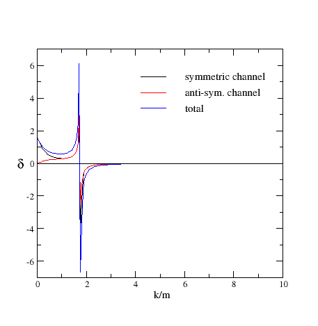
where the prime denotes the spatial derivative. The solution to this differential equation is subject to the boundary conditions $\beta(k,\infty)=\beta^{\prime}(k,\infty)=0$. The vacuum energy can now be computed from the standard spectral formula, provided that the phase shifts are defined through the Jost function in the conventional way. We consider symmetric potentials $V(x)=V(-x)$ and decompose the scattering problem on the real axis into two scattering problems on the half–axis $x\geq 0$. The phase shifts in the anti- and symmetric channels are respectively given by

$$\delta_{-}(k) =-\frac{1}{2}\,\mathsf{Re}\,\lim_{x\to 0}\,\Big{[}\beta(k,x)-\beta(-k,x)\big{]}$$

$$\delta_{+}(k) =\delta_{-}(k)+\frac{1}{2}\,\mathsf{Im}\,\lim_{x\to 0}\,\ln\frac{\beta^{\prime}(-k,x)-k}{\beta^{\prime}(k,x)+k}\,.$$ (60)

The combinations of Eq. (59) and (60) allows us to compute the total phase shift $\delta(k)=\delta_{+}(k)+\delta_{-}(k)$, which then yields the vacuum energy from Eq. (10), after integration by parts using Levinson’s theorem Graham et al. (2002),

$$E_{\rm vac}=-\int_{0}^{\infty}\frac{dk}{2\pi}\,\frac{k}{\sqrt{k^{2}+m^{2}}}\,\delta(k)+\frac{1}{2}\sum_{n}\big{(}|\omega_{n}|-m\big{)}\,.$$ (61)

Eqs. (59)–(61) are a complete system to compute the vacuum energy $E_{\rm vac}$ in the effective model using the local approximation. The only numerical issue arises due to the pole in Eq. (59) at threshold, $k_{T}=\sqrt{M^{2}-m^{2}}$. Our field theoretic derivation in Minkowski space has provided the correct $i\epsilon$-prescription to circumvent this pole, but it is still possible that the direct limit $\epsilon\searrow 0$ is numerically infeasible. To settle this issue, we have taken a sample background profile

$$V(x)=m\,c\,e^{-(mx/a)^{2}}\,,$$ (62)

with numerical constants $a$ and $b$. Table 1 shows results obtained for $c=1$, $a=2$ with masses $M/m=2$ and the threshold at $k_{T}/m=\sqrt{3}$. The integrals in the table correspond to the relevant integral in Eq. (61) — up to a factor of $1/(2\pi)$ — but now taken in a finite range covering the threshold, i.e. $I_{L}$ covers the range $k\in[3m/2,k_{T}]$, while $I_{R}$ refers to $[k_{T},2m]$. We then take $\epsilon=10^{-n}$ and increase $n$ to let $\epsilon\to 0$. As can be clearly seen, both integrals saturate around $n=8$, i.e. the limit $\epsilon\to 0$ in Eq. (59) can be taken literally. Figure 1 shows the resulting phase shifts for a value $\epsilon=10^{-10}$, where the numerics have converged.

Figure 1: Phase shifts for $\epsilon=10^{-10}$, $a=2$, $c=1$, and $M/m=2$; the threshold pole is at $k_{T}/m=\sqrt{3}$.

$n$	2	3	4	5	6	7	8	9	10
$\,\,\,I_{L}\,\,\,$	0.499	0.605	0.660	0.687	0.700	0.706	0.709	0.710	0.711
$I_{R}$	-0.642	-0.652	-0.653	-0.653	-0.653	-0.653	-0.653	-0.653	-0.653

Table 1: The left and right integrals explained in the main text, as functions of the position of the pole, $\epsilon=10^{-n}$. The model parameters are as in figure 1.

Next, we turn to the vacuum energy in the full model, Eq. (43). This is a simple coupled channel problem which is discussed at length in the literature Chadan and Sabatier (1977); Newton (1982). The idea is to write down the field equations for the vector $(\varphi,\Phi)$ and then put two of the four linear independent vector solutions (labeled by subscripts 1,2) in the columns of a $(2\times 2)$ matrix $\mathcal{F}$,

$$\begin{pmatrix}\varphi_{1}&\varphi_{2}\cr\Phi_{1}&\Phi_{2}\end{pmatrix}=\mathcal{F}\cdot\begin{pmatrix}{\rm e}^{ikx}&0\cr 0&{\rm e}^{iKx}\end{pmatrix}\,.$$ (63)

The other two solutions are obtained by complex conjugation because the original wave–equation (51) is real. The matrix $\mathcal{F}$ is suitable for a scattering problem because it parameterizes out–going plane waves with the boundary conditions $\mathcal{F}=1$ and $\mathcal{F}^{\prime}=0$ at spatial infinity. For a fixed energy $\omega$, it obeys the differential equation

$$\mathcal{F}^{\prime\prime}(x)=\begin{pmatrix}0&V(x)\\ V(x)&0\end{pmatrix}\cdot\mathcal{F}(x)-2i\mathcal{F}^{\prime}(x)\cdot\begin{pmatrix}k&0\\ 0&K\end{pmatrix}+\left[\mathcal{F}(x)\,,\,\begin{pmatrix}k^{2}&0\\ 0&K^{2}\end{pmatrix}\right]$$ (64)

where $k=\sqrt{\omega^{2}-m^{2}}$ and $K=\sqrt{\omega^{2}-M^{2}}$ above threshold, and $K=i\sqrt{M^{2}-\omega^{2}}$ below threshold. The latter case produces an exponential decay for $\Phi$ at large distances, and thus ensures that no flux occurs in this channel below threshold. In the antisymmetric channel, we find the $S$-matrix and phase shift, respectively, from the Jost solution to Eq. (64)

$$\mathcal{S}_{-}=\lim_{x\to 0}\mathcal{F}^{-1}\cdot\mathcal{F}^{\ast}\qquad{\rm and}\qquad\delta_{-}=\frac{-i}{2}\,\ln\mathrm{det}\,\mathcal{S}\,.$$ (65)

In principle, we should compute the phase shift below threshold only from the open channel, $\delta_{-}=(-i/2)\,\ln\left(\mathcal{S}_{-}\right)_{11}$. Eq. (65) still works in this regime, because $\left(\mathcal{S}_{-}\right)_{21}=0$ and $\left(\mathcal{S}_{-}\right)_{22}=1$.

In the symmetric channel, the situation is slightly more complicated. From the requirement that the derivative of the wave–function vanishes at the origin, we find

$$\mathcal{S}_{+}=-\lim_{x\to 0}\,\left[\mathcal{F}^{\prime}+\mathcal{F}\,\begin{pmatrix}ik&0\\ 0&iK\end{pmatrix}\right]^{-1}\cdot\left[{\mathcal{F}^{\ast}}^{\prime}-\mathcal{F}^{\ast}\,\begin{pmatrix}ik&0\\ 0&iK\end{pmatrix}\right]\,.$$ (66)

Again, $\delta_{+}=(-i/2)\,\ln\det\mathcal{S}_{+}$ above threshold, and $\delta_{+}=(-i/2)\,\ln\left(\mathcal{S}_{+}\right)_{11}$ below. This time, however, $\left(\mathcal{S}_{+}\right)_{22}=-1$ below threshold and we have to add an extra constant in $\delta_{+}=-\pi/2-i/2\,\ln\det\mathcal{S}_{+}$.

Figure 2: Comparison of the phase shifts in full and effective models for low energies. In the symmetric channel $\delta\to\pi/2$ as $\omega\to m$, suggesting a single bound state. The model parameters are $M/m=4$, $a=2$ and $c=1$.

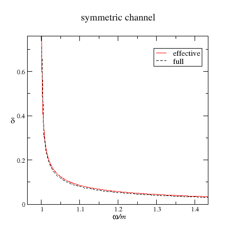
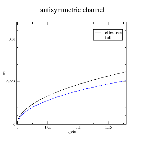
Figure 2 compares the low energy phase shifts in the full and effective model for the background potential Eq. (62) with $M/m=4$. As can be seen, the local approximation works fairly well at low energies, even if $M$ is not dramatically larger than $m$.

Finally, we compare the vacuum energies of the full and the effective model, which we split into continuum and bound state contributions according to Eqs. (10) and (61). The bound states can be computed by a variety of methods such as shooting, direct diagonalization of the Schrödinger operator in a suitable function basis, or from the roots of the Jost function at imaginary momentum $k=i\kappa$. In all methods we find, besides the usual bound states, formal solutions with $\omega^{2}<0$ as well. These solutions represent unphysical states with an amplitude increasing exponentially in time, i.e. they are undamped resonances that must not be included in the vacuum energy, although they are required to satisfy Levinson’s theorem, which merely counts the number of roots of the Jost function in $k$–space.

In table 2, we have listed the vacuum energy (in units of $m$) for our preferred background Eq. (62) and $a=2$, $c=6$. As can be seen, there is still a considerable difference between the full and exact model, especially for small mass ratios $M/m$. The discrepancy is almost completely due to the continuum contribution $E_{\delta}$, whose relative error decreases significantly as $M/m$ gets larger. Unfortunately, the numerics become very delicate for larger masses, because the exponential damping ${\rm e}^{-|K|x}$ becomes very small and cannot be accurately compared to data of order one.

$\quad M/m\quad$	$\quad E_{\delta}\quad$	$E_{\text{bs}}^{2}(\text{sym})$	$E_{\text{bs}}^{2}(\text{asym})$	$\quad E_{\text{vac}}\quad$
2	-0.20	-2.58 ; 0.77	-0.60	-0.26
3	0.29	-1.22	0.42	0.11
4	0.36	-0.29	0.88	0.33
5	0.32	0.23	0.99	0.06
6	0.27	0.52	$0.99^{\ast}$	0.13
7	0.22	0.68	$0.99^{\ast}$	0.13

$\quad M/m\quad$	$\quad E_{\delta}\quad$	$E_{\text{bs}}^{2}(\text{sym})$	$E_{\text{bs}}^{2}(\text{asym})$	$\quad E_{\text{vac}}\quad$
2	0.75	-2.83 ;-0.08	-1.27; 0.77	0.69
3	0.80	-1.34	0.18	0.51
4	0.65	-0.34	0.83	0.60
5	0.52	0.21	$0.99^{\ast}$	0.25
6	0.41	0.51	$0.99^{\ast}$	0.26
7	0.33	0.68	$0.99^{\ast}$	0.24

Table 2: Contributions to the vacuum energy for the full model (left) and the effective model (right) at various mass ratios $M/m$. Parameters for the background coupling are $a=2$, $c=6$ and all energies are given in units of the light meson mass $m$. The phase shift contribution $E_{\delta}$ refers to the binding energy, Eq. (61). Bound state energies are given as absolute values. The vacuum energy is given by $E_{\rm vac}=E_{\delta}+\frac{1}{2}\,\sum_{n}\big{(}|E_{\rm bs}|-m\big{)}$ , where the sum only includes true bound states with $E_{\rm bs}^{2}>0$. Asterisks mark bound states that have not been found numerically since they are too close to threshold. They must exist because of Levinson’s theorem and they must have binding energies of less than $0.01$ since our numerical algorithm would have detected them otherwise. Numerically, their contribution to the vacuum energy is hence negligible.

V Dielectric

The introduction of a permeability, $\mu$ and a permittivity, $\epsilon$ to describe the interaction of electromagnetic fields with matter is a prime example for an effective model. It arises from integrating out the microscopic matter degrees of freedom of the fundamental QED formulation and leads to the Maxwell equations in matter

$$\nabla\cdot\mathbf{D}=4\pi\rho\,,\qquad\qquad\nabla\times\mathbf{E}+\partial_{t}\mathbf{B}=0\,,\qquad\qquad\nabla\cdot\mathbf{B}=0\qquad{\rm and}\qquad\nabla\times\mathbf{H}-\partial_{t}\mathbf{D}=4\pi\mathbf{j}\,,$$ (67)

where $\mathbf{D}(t,\mathbf{x})=\int dt^{\prime}\epsilon(t^{\prime},\mathbf{x})\,\mathbf{E}(t-t^{\prime},\mathbf{x})$ and $\mathbf{B}(t,\mathbf{x})=\int dt^{\prime}\mu(t^{\prime},\mathbf{x})\,\mathbf{H}(t-t^{\prime},\mathbf{x})$ and information about the charge carriers in the material is contained in the phenomenological quantities $\mu$ and $\epsilon$. For simplicity we restrict our attention to the case of $\mu=1$.

We are interested in vacuum polarization energies so there are no external charges or currents and we set $\rho=0$ and $\mathbf{j\,}=0$. Frequency dependence arises in this model in two ways: first, via the explicit time derivatives in Eq. (67), which generate factors of frequency multiplying the interaction, and second via the frequency dependence of the dielectric function $\epsilon$ itself. The latter arises because the response of any realistic material must go to zero for large frequency. Furthermore, by the Kramers–Kronig relations, enforcing causality requires that a frequency-dependent dielectric function have a nontrivial imaginary part, representing dissipation.

Of course, electromagnetic Casimir fluctuations do not lead to energy dissipation in a dielectric material; they exist in equilibrium with fluctuations in the microscopic matter degrees of freedom. Such an effective model can be described by a partition function in quantum statistical mechanics, but not by a canonical quantum field theory, since it lacks a strictly conserved energy. In the statistical mechanics approach Rahi et al. (2009); Kenneth and Klich (2006, 2008), the partition function is defined on the imaginary frequency axis, where the dielectric function is strictly real (even with dissipation). Because the nonlocality in time introduced by the frequency dependence in $\epsilon$ always takes the form of a convolution, one can factorize the problem according to frequency. To compute the partition function, one then integrates over all field configurations; this integral is dominated by contributions arising from the saddle-point integration around each solution to the classical equation of motion for a fixed frequency. From the partition function one obtains the free energy, which at $T=0$ gives the Casimir energy as a statistical ensemble average. This is the approach that has been adopted in Refs. Rahi et al. (2009); Kenneth and Klich (2006, 2008). By relating the resulting functional integral to the free energy one finds an energy density given by the integral over space of $\frac{1}{2}(\mathbf{E}\cdot\mathbf{D}+\mathbf{B}^{2})$. The saddle point approximation to this functional integral gives the fields as solutions to Maxwell’s equations in matter. This statistical mechanics picture for the energy is consistent with the classical thermodynamics result that fluctuations of the charge density due to exposure to an electric field contribute the spatial integral of $\frac{1}{2}\mathbf{E}\cdot\mathbf{D}$ to the free energy Panofsky and Phillips (1962); Jackson (1975). The problem is stationary and it is suitable to introduce Fourier modes $\mathbf{E}_{k}(\mathbf{x})=\int dt\,{\rm e}^{ikt}\,\mathbf{E}(\mathbf{x},t)$ and $\mathbf{B}_{k}(\mathbf{x})=\int dt\,{\rm e}^{ikt}\,\mathbf{B}(\mathbf{x},t)$. Their contributions to the energy are then summed over frequency $k$. The frequency dependence in the interaction then leads to additional terms in the relation (8) between the integrated wave–function and the Jost function for imaginary frequencies, as described in Ref. Graham et al. (2013). In this case, we obtain the Casimir energy of a single Fourier mode from the integral over space of

$$u_{I}(\mathbf{x})=\frac{1}{2}\epsilon_{k}\mathbf{E}_{k}^{2}+\frac{1}{2}\mathbf{B}_{k}^{2}\,.$$ (68)

Here, we will follow an alternative path at the cost of violation of the Kramers–Kronig relations. We will stay within quantum field theory to consider a conserved energy that is derived from Maxwell’s equations in matter (67). As outlined in the appendix, it is an awkward expression in coordinate space. However, when expressed in terms of the Fourier modes, it takes a compact from, that e.g. has been used in Refs. Milton et al. (2010); Rosa et al. (2010, 2011), see Eq. (69) below. We will find that in this case, the additional terms in the relationship between the Jost function and the integrated wave–functions cancel with the additional terms in the energy expression, leaving the same expressions as arise for a frequency–independent potential. In this case, we can carry out a derivation within field theory and find the strictly conserved energy to be the integral over space of

$$u_{II}(\mathbf{x})=\frac{1}{2}\frac{\partial[k\epsilon_{k}]}{\partial k}\,\mathbf{E}_{k}^{2}+\frac{1}{2}\mathbf{B}_{k}^{2}\,.$$ (69)

Both Eqs. (68) and (69) give the contribution of a single mode. Formally the time-independence of $\int d^{3}x\,u_{II}(\mathbf{x})$ can be verified for all cases in which $\epsilon_{k}$ has a Taylor expansion in $k^{2}$, but not $k$. This condition is, however, not fulfilled by any physically motivated dielectric functions such as Eq. (77) below. In particular, this sort of Taylor expansion is not compatible with the Kramers–Kronig relations for spectral functions. Nevertheless this case allows us to investigate the effect of frequency dependent interactions in the context of spectral methods applied to vacuum energies.

Assuming a spherically symmetric dielectric $\epsilon_{k}(r)=\int dt\,{\rm e}^{ikt}\,\epsilon(t,\mathbf{x})$ leads to the so–called Mie–model Mie (1908); Newton (1982). With these preliminaries Maxwell’s equations (67) can be transformed into decoupled second order differential equations for scalar fields $\varphi_{k}(\mathbf{x})$ and $\phi_{k}(\mathbf{x})$ by the ansätze

$${\rm TE:}\qquad \mathbf{E}_{k}(\mathbf{x})=k\,\nabla\times[\varphi_{k}(\mathbf{x})\,\mathbf{x}]\qquad{\rm and}\qquad \mathbf{B}_{k}(\mathbf{x})=i\nabla\times\left(\nabla\times\left[\varphi_{k}(\mathbf{x})\,\mathbf{x}\right]\right)$$ (70)

$${\rm TM:}\qquad \mathbf{B}_{k}(\mathbf{x})=-ik\,\nabla\times\left[\phi_{k}(\mathbf{x})\,\mathbf{x}\right]\qquad{\rm and}\qquad \mathbf{E}_{k}(\mathbf{x})=\frac{-1}{\epsilon_{k}(r)}\nabla\times\left(\nabla\times\left[\phi_{k}(\mathbf{x})\,\mathbf{x}\right]\right)\,,\hskip 85.35826pt$$ (72)

for the transverse electric (TE) and transverse magnetic (TM) modes, respectively. The spherical decompositions (with angular momentum channels $\ell=1,2,\ldots$)

$$\varphi_{k,\ell m}(\mathbf{x})=\frac{1}{\sqrt{\ell(\ell+1)}}Y_{\ell}^{m}(\theta,\phi)\frac{1}{r}f_{k,\ell}(r)\qquad{\rm and}\qquad\phi_{k,\ell m}(\mathbf{x})=\frac{\sqrt{\epsilon_{k}(r)}}{\sqrt{\ell(\ell+1)}}Y_{\ell}^{m}(\theta,\phi)\frac{1}{r}g_{k,\ell}(r)$$ (73)

allow to consistently compute scattering data for a fixed frequency $k$ from the differential equations

$$k^{2}\epsilon_{k}(r)f_{k,\ell}(r) = -f_{k,\ell}^{\prime\prime}(r)+\frac{\ell(\ell+1)}{r^{2}}f_{k,\ell}(r)\qquad{\rm and}$$ (74)

$$k^{2}\epsilon_{k}(r)g_{k,\ell}(r) = -g_{k,\ell}^{\prime\prime}(r)+\frac{\ell(\ell+1)}{r^{2}}g_{k,\ell}(r)+\left[\frac{3\epsilon_{k}^{\prime 2}(r)}{4\epsilon_{k}^{2}(r)}-\frac{\epsilon_{k}^{\prime\prime}(r)}{2\epsilon_{k}(r)}\right]g_{k,\ell}(r)\,,$$ (76)

where primes denote derivatives with respect to the radial coordinate. We have also elevated the permittivity to a dielectric function of the frequency $k$ and indicated that by a subscript. This frequency dependence is unavoidable to maintain the renormalizability which should be preserved because it is manifest in the underlying quantum electrodynamics. From scattering theory we know that a non–trivial metric, as represented by the left hand sides of Eqs. (76), leads to linearly rising phase shifts at large $k$. This increase cannot be compensated by any finite number of Born subtractions. In the language of Feynman diagrams it corresponds to a quadratic derivative interaction with the background. Multiplying such a vertex with a propagator approaches a constant in the ultra–violet producing infinitely many divergent diagrams. Hence, to maintain renormalizability, the deviation of the dielectric function from unity must vanish like $1/k^{2}$ at large frequencies. Note that this reasoning is similar as for the effective model considered in section IV. The dielectric function is commonly parameterized in terms of the imaginary frequency $\kappa=-ik$,

$$\epsilon_{i\kappa}(r)=1+\frac{p(r)}{\kappa^{2}\lambda^{2}+\frac{\pi}{\sigma_{P}}\kappa}\,,$$ (77)

where $\lambda$ is the so–called plasma wave–length whose inverse corresponds to a material cut–off in the ultra–violet according to the above discussion. Furthermore, $\sigma_{P}$ is the conductivity whose main purpose in the context of Casimir energy calculations is to circumvent infra–red divergences. If the spherically symmetric profile function $p(r)$ is strongly peaked at a specified radius, the above is a well–suited effective model for the interaction of photons with a dielectric sphere.

Angular integration yields the radial energy densities (omitting the angular momentum label for simplicity)

$$2u_{I}^{\rm(TE)}(k,r) = \epsilon_{k}(r)k^{2}f_{k}^{2}(r)+[(rf_{k}(r))^{\prime}]^{2}+\ell(\ell+1)f_{k}^{2}(r)$$ (78)

$$2u_{I}^{\rm(TM)}(k,r) = g_{k}^{\prime 2}(r)+\frac{\epsilon_{k}^{\prime}(r)}{\epsilon_{k}(r)}g_{k}(r)g_{k}^{\prime}(r)+\frac{\epsilon^{\prime 2}_{k}(r)}{4\epsilon_{k}^{2}(r)}g_{k}^{2}(r)+\frac{\ell(\ell+1)}{r^{2}}g_{k}^{2}(r)+k^{2}\epsilon_{k}(r)g_{k}^{2}(r)$$ (80)

and

$$2u_{II}^{\rm(TE)}(k,r) = k^{2}\left[\epsilon_{k}(r)+k\dot{\epsilon}_{k}(r)\right]f_{k}^{2}(r)+[(rf_{k}(r))^{\prime}]^{2}+\ell(\ell+1)f_{k}^{2}(r)$$ (81)

$$2u_{II}^{\rm(TM)}(k,r) = \left[1+k\frac{\dot{\epsilon}_{k}(r)}{\epsilon_{k}(r)}\right]\left[g_{k}^{\prime 2}(r)+\frac{\epsilon^{\prime}_{k}(r)}{\epsilon_{k}(r)}g_{k}(r)g_{k}^{\prime}(r)+\frac{\epsilon^{\prime 2}_{k}(r)}{4\epsilon^{2}_{k}(r)}g_{k}^{2}(r)+\frac{\ell(\ell+1)}{r^{2}}g_{k}^{2}(r)\right]+k^{2}\epsilon_{k}(r)g_{k}^{2}(r)$$ (83)

for the two candidates of Eqs. (68) and (69). In contrast to the previous sections the dot now denotes a derivative with respect to frequency, $\dot{\epsilon}_{k}=\partial\epsilon_{k}/\partial k$. Using the differential equations (76) and omitting total space derivative terms simplifies the densities considerably in case ($I$) Graham et al. (2013)

$$u_{I}^{\rm(TE)}(k,r)=\epsilon_{k}(r)k^{2}f_{k}^{2}(r)\qquad{\rm and}\qquad u_{I}^{\rm(TM)}(k,r)=\epsilon_{k}(r)k^{2}g_{k}^{2}(r)\,,$$ (84)

but not in case ($II$)

$$u_{II}^{\rm(TE)}(k,r) = k^{2}\left[\epsilon_{k}(r)+\frac{k}{2}\dot{\epsilon}_{k}(r)\right]f_{k}^{2}(r)$$ (85)

$$u_{II}^{\rm(TM)}(k,r) = k^{2}\left[\epsilon_{k}(r)+\frac{k}{2}\dot{\epsilon}_{k}(r)\right]g_{k}^{2}(r)+\frac{k}{4}\left[\frac{\dot{\epsilon}^{\prime\prime}_{k}(r)}{\epsilon_{k}(r)}-3\frac{\dot{\epsilon}^{\prime}_{k}(r){\epsilon}^{\prime}_{k}(r)}{\epsilon^{2}_{k}(r)}-\frac{\dot{\epsilon}_{k}(r){\epsilon}^{\prime\prime}_{k}(r)}{\epsilon^{2}_{k}(r)}+3\frac{\dot{\epsilon}_{k}(r){\epsilon}^{\prime 2}_{k}(r)}{\epsilon^{3}_{k}(r)}\right]g_{k}^{2}(r)\,.$$ (87)

In the next step we want to express the energy density by scattering data. As previously, cf. Eqs. (6), (40) and (56), we start by computing the Wronskian between the regular and Jost solutions at different frequencies. This involves the field equations (76) from which we identify

$$U_{k}^{\rm(TE)}(r)=k^{2}\left[1-\epsilon_{k}(r)\right]\qquad{\rm and}\qquad U_{k}^{\rm(TM)}(r)=k^{2}\left[1-\epsilon_{k}(r)\right]+\left[\frac{3\epsilon_{k}^{\prime 2}(r)}{4\epsilon_{k}^{2}(r)}-\frac{\epsilon_{k}^{\prime\prime}(r)}{2\epsilon_{k}(r)}\right]$$ (88)

to be substituted into, say, Eq. (56). It remains to compare the frequency derivatives

$$-\frac{\partial}{\partial k}\left[k^{2}+U_{k}^{\rm(TE)}(r)\right] = 2k\epsilon_{k}(r)+k^{2}\dot{\epsilon}_{k}(r)\qquad{\rm and}\qquad$$ (89)

$$-\frac{\partial}{\partial k}\left[k^{2}+U_{k}^{\rm(TM)}(r)\right] = 2k\epsilon_{k}(r)+k^{2}\dot{\epsilon}_{k}(r)-\frac{3\dot{\epsilon}^{\prime}_{k}(r)\epsilon^{\prime}_{k}(r)}{2\epsilon^{2}_{k}(r)}+\frac{3\dot{\epsilon}_{k}(r)\epsilon^{\prime 2}_{k}(r)}{2\epsilon^{3}_{k}(r)}+\frac{\dot{\epsilon}^{\prime\prime}_{k}(r)}{2\epsilon_{k}(r)}-\frac{\dot{\epsilon}_{k}(r)\epsilon^{\prime\prime}_{k}(r)}{2\epsilon^{2}_{k}(r)}$$ (91)

with the coefficient functions in the expressions for energy densities. Obviously there are significant differences in case ($I$) but up to the additional factor $k/2$ it agrees with the formula for the energy density in case ($II$). This implies that the latter case will have the standard phase shift expression for the vacuum polarization energy, Eq. (4) while case ($I$) has additional contributions. These contributions have been studied in Ref. Graham et al. (2013) for a dielectric sphere and were found to yield an attractive force.

To summarize this section, we have shown that in the absence of dissipation, we have a formulation that is rigorous and well founded in quantum field theory, while in the presence of dissipation such a full quantum field theory formulation is not available and we need to resort to a statistical mechanics approach. In the latter case one employs the conventional expression for the energy with a constant dielectric (type ($I$)), which leads to extra terms in our spectral analysis, while the unconventional form ($II$), that one obtains in the former case, does not.

VI Conclusions

We have discussed several models in which quantum fluctuations interact with a (static) background through frequency dependent couplings. In such scenarios the conjugate field momenta, and thus all observables computed as Noether charges, involve the interaction explicitly, rather than only intrinsically via the solutions to the wave–equation. Furthermore it is not obvious that energy and action functionals of even static configurations are proportional. We have therefore studied the question whether the simple phase shift formula, Eq. (3), for the vacuum polarization energy remains valid in such cases. On top of the arguments above, the validity of this formula is not at all evident since the major ingredients for its derivation in the frequency independent case no longer hold: On the (canonical) quantum field theory side we must re–examine the relationship between the energy density and the Green’s function, while on the scattering problem side we must re–consider the relationship between the derivative of the phase shift and the appropriate spatial integral over the Green’s function. Modifications may arise because this relationship is deduced from the derivative of the wave–equation with respect to frequency.

In an effective model the frequency dependence is commonly non–polynomial , which prevents us from applying canonical quantization. As a result, statements about the vacuum expectation values of the energy can only be made by comparison with classical analogs.

In the simplest of all possible models with frequency dependent interactions, scalar electrodynamics, the phase shift formula continues to hold because the modifications on the field theory and scattering sides compensate each other. In effective models which emerge from integrating out fundamental degrees of freedom, approximations that ignore the frequency dependence usually spoil renormalizability and thus must be avoided in the context of quantum energies. As seen in the simple model of section IV, the resulting frequency dependence in the effective theory is non–polynomial. This makes it difficult to construct a conserved energy functional from the wave–equations from within the effective model. Generally, such a construction is possible only when the wave–equation is a polynomial of the frequency squared, cf. appendix A.

In the model we considered, we were fortunate enough to be able to trace the energy functional from the fundamental theory. When we applied the same approximation to the energy density as for the wave–equation when integrating out the heavier field, we observed that the phase shift formula also holds in such a scenario. This result comes about because the local approximation to the energy density gives the same result as the polynomial construction principle applied to the wave–equation in the local approximation. After obtaining this result formally in the effective model we have also verified it numerically by comparing to the full theory in the regime where the adopted approximations are valid.

As a third example we have considered the physically interesting problem of a dielectric. The relevant wave–equations are Maxwell’s equation in matter. Assuming spherical symmetry for the background leads to the Mie model. This formulation represents an effective model because the fundamental interactions between the charge carriers and quantum fluctuations of the electromagnetic field are imitated phenomenologically. We have compared two formulations of this effective theory. When we include dissipation, as required by the Kramers–Kronig relations, we do not have a quantum field theory formulation of the problem. Instead a statistical mechanics ensemble average Rahi et al. (2009); Kenneth and Klich (2006, 2008) leads to an energy density of type ($I$) with the ensuing extra terms in the phase shift formula. They can then play an important role in the calculation of Casimir self–stresses Graham et al. (2013). Without dissipation, a Taylor expansion in the frequency squared is permitted and a conserved quantity can be constructed from the wave–equation, leading to an energy density of type ($II$), which does not lead to extra terms in the phase shift analysis. For forces between rigid bodies the situation is simpler, since one can consider the stress tensor $T_{\mu\nu}$ outside the dielectric, where $T_{\mu\nu}$ is uniquely defined and the fields are obtained from the Mie equation.

Appendix A Energy from Wave–Equation

In this appendix we explain the statement of section V concerning the derivation of an energy functional when the wave–equation has a Taylor expansion in the frequency squared. This analysis is based on analogies with classical systems.

Let $\phi_{k}(\mathbf{x})$ be a solution to the wave–equation with frequency $k$. We assume that the wave–equation only contains even powers of $k$

$$\left(k^{2}+\alpha_{2}k^{4}+\alpha_{3}k^{6}+\ldots\right)\phi_{k}=\hat{O}\phi_{k}\,.$$ (92)

Here $\alpha_{i}$ may be spatial functions and $\hat{O}$ is some Hermitian operator that contains a static potential and perhaps some spatial derivatives. Let us consider a term like $k^{2n}\phi_{k}(\mathbf{x})$. In coordinate space it amounts to $(-1)^{n}\partial_{t}^{2n}\phi(t,\mathbf{x})$. We choose the overall sign such that the standard $n=1$ term has a positive coefficient, multiply this term by $\partial_{t}\phi(t,\mathbf{x})$ and identify a total derivative:

$$(-1)^{n+1}\left(\partial_{t}\phi\right)\left(\partial_{t}^{2n}\phi\right) = (-1)^{n+1}\left\{\partial_{t}\left[\left(\partial_{t}\phi\right)\left(\partial_{t}^{2n-1}\phi\right)\right]-\left(\partial_{t}^{2}\phi\right)\left(\partial_{t}^{2n-1}\phi\right)\right\}$$ (93)

$$= (-1)^{n+1}\left\{\partial_{t}\left[\left(\partial_{t}\phi\right)\left(\partial_{t}^{2n-1}\phi\right)\right]-\partial_{t}\left[\left(\partial_{t}^{2}\phi\right)\left(\partial_{t}^{2n-2}\phi\right)\right]+\left(\partial_{t}^{3}\phi\right)\left(\partial_{t}^{2n-2}\phi\right)\right\}$$ (95)

$$\vdots$$ (97)

$$= (-1)^{n}\left\{\partial_{t}\sum_{j=1}^{n-1}(-1)^{j}\left(\partial_{t}^{j}\phi\right)\left(\partial_{t}^{2n-j}\phi\right)+(-1)^{n}\left(\partial_{t}^{n}\phi\right)\left(\partial_{t}^{n+1}\phi\right)\right\}$$ (99)

$$= \partial_{t}\left\{\sum_{j=1}^{n-1}(-1)^{j+n}\left(\partial_{t}^{j}\phi\right)\left(\partial_{t}^{2n-j}\phi\right)+\frac{1}{2}\left(\partial_{t}^{n}\phi\right)\left(\partial_{t}^{n}\phi\right)\right\}\,.$$ (101)

Hence we identify the contribution to the density of the conserved energy as

$$u_{n}(t,\mathbf{x})=\sum_{j=1}^{n-1}(-1)^{j+n}\left(\partial_{t}^{j}\phi\right)\left(\partial_{t}^{2n-j}\phi\right)+\frac{1}{2}\left(\partial_{t}^{n}\phi\right)\left(\partial_{t}^{n}\phi\right)\,.$$ (102)

In frequency space the energy density is a double integral over $k$ and $k^{\prime}$, $u_{n}(t,\mathbf{x})=\int\frac{dk}{2\pi}\int\frac{dk^{\prime}}{2\pi}\phi_{k^{\prime}}\left[\ldots\right]\phi_{k}{\rm e}^{i(k+k^{\prime})t}$, where the ellipsis replaces the frequency representation of the operators in Eq. (102). Then the vacuum matrix element projects this bilocal object onto its diagonal ($k=-k^{\prime}$) terms in a similar way, since they contribute solely to the total energy $\int d^{3}x\sum_{n}u_{n}(t,\mathbf{x})$; that calculation is provided below (classically one can argue that energy conservation allows one to average over time, which also implements this projection). The diagonal projection becomes time-independent,

$$\tilde{u}_{n}(k) = (-1)^{n}\phi_{-k}\left\{\sum_{j=1}^{n-1}(-1)^{j}\left(ik\right)^{j}\left(-ik\right)^{2n-j}+\frac{1}{2}(-1)^{n}\left(ik\right)^{n}\left(-ik\right)^{n}\right\}\phi_{k}$$ (103)

$$= (-1)^{n}\phi_{-k}\left\{\sum_{j=1}^{n-1}(i)^{2n}k^{2n}+\frac{1}{2}(-1)^{n}k^{2n}\right\}\phi_{k}=\frac{1}{2}\phi_{-k}\left(2n-1\right)k^{2n}\phi_{k}=\frac{1}{2}\phi_{-k}\left\{k^{2}\partial_{k}\left(k^{2n-1}\right)\right\}\phi_{k}\,,$$ (105)

where the last equation relates to the type ($II$) energy of section V and we have not written the frequency integral explicitly. To show that this construction does not work for odd powers of the frequency we merely need to consider

$$\left(\partial_{t}\phi\right)\left(\partial_{t}^{3}\phi\right)=\partial_{t}\left[\left(\partial_{t}\phi\right)\left(\partial_{t}^{2}\phi\right)\right]-\left(\partial_{t}^{2}\phi\right)\left(\partial_{t}^{2}\phi\right)\,.$$ (106)

The second term on the right hand side cannot be expressed as a total derivative and further application of the product rule merely yields a trivial identity. In the case of scalar electrodynamics (section II) a complex quantum field was studied. Models that couple odd powers of the frequency via different field components are permissible. It is also obvious that the construction does not straightforwardly apply to a non–polynomial dependence on frequency either, because the product rule cannot be used. Such a dependence, however, is essential for a renormalizable model.

The frequency independent term on the right hand side of Eq. (92) contributes $\frac{1}{2}\int d^{d}x\,\phi_{-k}\hat{O}\phi_{k}$ to the energy. This contribution can be expressed via the wave–equation (92) and adds $(1/2)\phi_{-k}\,\alpha_{n}k^{2n}\,\phi_{k}$ to $\tilde{u}_{n}$, cf. Eq. (50). This changes the coefficient in Eq. (105) to

$$\frac{1}{2}(2n-1)k^{2n}+\frac{1}{2}k^{2n}=k^{2}\frac{\partial}{\partial k^{2}}\,k^{2n}\,.$$ (107)

Said another way, once the potential type contribution to the energy has been eliminated via the wave–equations, the energy factor is given by $k^{2}\frac{\partial}{\partial k^{2}}\,V_{k}(\mathbf{x})$, where $V_{k}(\mathbf{x})$ represents the complete frequency dependence in the wave–equation. In this way Eqs. (52) and (54) are consistent. The application of this prescription to Eq. (76) yields Eq. (83). We also note that this result is kindred to the frequency derivatives that appear in the derivation of the phase shift formula after Eqs. (6), (40) and (57) since $k^{2}\frac{\partial}{\partial k^{2}}\,V_{k}(\mathbf{x})=\frac{k}{2}\frac{\partial}{\partial k}\,V_{k}(\mathbf{x})$.

In the context of Eq. (105) we have noted that the energy density is bilocal in frequency but only the diagonal projection is relevant for the total energy. This projection arises from the orthogonality condition between solutions with different frequencies. Again assuming that $V_{k}(\mathbf{x})$ is even in $k$, this condition reads

$$\int d^{d}xf_{k^{\prime}}(\mathbf{x})\frac{V_{k}(\mathbf{x})-V_{k^{\prime}}(\mathbf{x})}{k^{2}-k^{\prime 2}}f_{k}(\mathbf{x})\propto\delta(k^{2}-k^{\prime 2})\,.$$ (108)

From the geometrical series identity

$$\frac{k^{2n}-k^{\prime 2n}}{k^{2}-k^{\prime 2}}(k-k^{\prime})^{2}=2\sum_{j=1}^{n-1}\left[(-k^{\prime})^{j}k^{2n-j}+(-k)^{j}k^{\prime 2n-j}\right]+2(-kk^{\prime})^{n}+k^{2n}+k^{\prime 2n}$$ (109)

one can verify order by order that the total energy constructed above indeed turns into a single frequency integral and is time independent. The first three terms on the right hand side of Eq. (109) arise from Eq. (102) after identifying $k$ and $k^{\prime}$. The last two stem from eliminating the explicit $\hat{O}$ contribution via the wave–equations. Furthermore, note that the metric factor for the normalization of the wave–function extracted from Eq. (108) in the limit $k^{\prime}\to k$ leads to the construction prescription for constructing the weight factor in the energy.

The above discussion was carried out for a simple scalar field. However, it is straightforwardly applied to electromagnetism in matter starting from the wave–equations

$$\nabla\times\mathbf{E}+\partial_{t}\mathbf{B}=0\qquad{\rm and}\qquad\nabla\times\mathbf{B}-\partial_{t}\left[\epsilon_{-i\partial_{t}}\mathbf{E}\right]=0$$ (110)

in coordinate space. Subtraction of the two equations after scalar multiplication of the first with $\mathbf{B}$ and the second with $\mathbf{E}$ yields a left hand side

$$\nabla\cdot\left(\mathbf{E}\times\mathbf{B}\right)=\mathbf{B}\cdot\partial_{t}\mathbf{B}+\mathbf{E}\cdot\partial_{t}\,\epsilon_{-i\partial_{t}}\mathbf{E}$$ (111)

which is the divergence of the Poynting vector and vanishes after spatial integration. If the dielectric function had the expansion $\epsilon_{-i\partial_{t}}=1+\sum_{n=1}^{N}\alpha_{n}\partial_{t}^{2n}$ the manipulations analogous to Eq. (101) would then suggest that the coordinate representation $\int d^{3}x\,u_{II}(t,\mathbf{x})$ is constant in time. Note that in Eq. (111) the potential type term $\phi\hat{O}\phi\sim\mathbf{B}^{2}$ has not yet been eliminated by the wave–equation. Thus we indeed require $\frac{\partial}{\partial k}(k\epsilon_{k})$ and not $\frac{\partial}{\partial k^{2}}(k^{2}\epsilon_{k})$ as the coefficient of $\mathbf{E}^{2}$.

As for the scalar case, the generalization of this construction to odd powers in the frequency requires mixing of components. This can be accomplished by a tensor relation between the displacement $\mathbf{D}$ and the electric field $\mathbf{E}$. In particular odd powers of the frequency must be accompanied by an anti–symmetric tensor. The feature of such an anti–symmetric internal structure is the disappearance of the left over term in Eq. (106). The simple example

$$\mathbf{D}=\mathbf{E}+{\boldsymbol{a}}\times\dot{\mathbf{E}}\,.$$ (112)

where ${\boldsymbol{a}}$ is some vector with dimension of time that may vary in space, illustrates this point. To construct a conserved quantity we again find the contribution to the divergence of the Poynting vector

$$\mathbf{E}\cdot\partial_{t}\mathbf{D}=\mathbf{E}\cdot\partial_{t}\left[\mathbf{E}+{\boldsymbol{a}}\times\dot{\mathbf{E}}\right]=\partial_{t}\left[\frac{1}{2}\mathbf{E}^{2}+\mathbf{E}\cdot({\boldsymbol{a}}\times\dot{\mathbf{E}})\right]\,.$$ (113)

The object in square brackets is the contribution to the energy density. In frequency space it has the diagonal projection

$$\frac{1}{2}(E_{-k})_{i}\left[\delta_{ij}-2ik\epsilon_{ilj}a_{l}\right](E_{k})_{j}\,,$$ (114)

which again has the kernel $\frac{\partial}{\partial k}(k\epsilon_{k})$ of $u_{II}$. Standard textbook Landau and Lifshitz (1986); Schwinger et al. (1998) derivations of this kernel consider electric fields that are a superposition of waves with frequencies in a small bandwidth. Obviously the arguments presented in this appendix do not rely on this simplifying assumption.

References

- Graham et al. (2009) N. Graham, M. Quandt, and H. Weigel, Lect.Notes Phys. 777, 1 (2009).
- Graham et al. (2002) N. Graham, R. L. Jaffe, V. Khemani, M. Quandt, M. Scandurra, and H. Weigel, Nucl. Phys. B645, 49 (2002).
- Rajaraman (1982) R. Rajaraman, Solitons and Instantons (North Holland, 1982).
- Faulkner (1977) J. S. Faulkner, J. Phys. C: Solid State Phys. 10, 4461 (1977).
- Graham et al. (2011) N. Graham, M. Quandt, and H. Weigel, Phys.Rev. D84, 025017 (2011),
- Farhi et al. (2000) E. Farhi, N. Graham, R. L. Jaffe, and H. Weigel, Nucl.Phys. B585, 443 (2000),
- Graham et al. (2001) N. Graham, R. L. Jaffe, M. Quandt, and H. Weigel, Phys.Rev.Lett. 87, 131601 (2001),
- Dashen et al. (1974) R. F. Dashen, B. Hasslacher, and A. Neveu, Phys.Rev. D10, 4114 (1974).
- Gervais et al. (1975) J.-L. Gervais, A. Jevicki, and B. Sakita, Phys.Rev. D12, 1038 (1975).
- Cahill et al. (1976) K. E. Cahill, A. Comtet, and R. J. Glauber, Phys.Lett. B64, 283 (1976).
- Nakahara and Maki (1982) M. Nakahara and K. Maki, Phys. Rev. B25, 7789 (1982).
- Graham and Jaffe (1999) N. Graham and R. L. Jaffe, Nucl.Phys. B544, 432 (1999),
- Flores-Hidalgo (2002) G. Flores-Hidalgo, Phys.Lett. B542, 282 (2002),
- Moussallam and Kalafatis (1991) B. Moussallam and D. Kalafatis, Phys.Lett. B272, 196 (1991).
- Meier and Walliser (1997) F. Meier and H. Walliser, Phys.Rept. 289, 383 (1997),
- Weigel (2008) H. Weigel, Lect.Notes Phys. 743, 1 (2008).
- Rahi et al. (2009) S. J. Rahi, T. Emig, N. Graham, R. L. Jaffe, and M. Kardar, Phys.Rev. D80, 085021 (2009),
- Kenneth and Klich (2006) O. Kenneth and I. Klich, Phys. Rev. Lett. 97, 160401 (2006).
- Kenneth and Klich (2008) O. Kenneth and I. Klich, Phys.Rev. B78, 014103 (2008),
- Graham et al. (2013) N. Graham, M. Quandt, and H. Weigel, Phys.Lett. B726, 846 (2013),
- Landau and Lifshitz (1986) L. D. Landau and E. M. Lifshitz, Electrodynamics of Continuous Media (Butterworth–Heinemann, 1986), chap. 80.
- Brevik and Milton (2008) I. H. Brevik and K. A. Milton, Phys.Rev. E78, 011124 (2008),
- Milton et al. (2010) K. A. Milton, J. Wagner, P. Parashar, and I. H. Brevik, Phys.Rev. D81, 065007 (2010),
- Rosa et al. (2010) F. S. S. Rosa, D. A. R. Dalvit, and P. W. Milonni, Phys. Rev. A 81, 033812 (2010).
- Rosa et al. (2011) F. S. S. Rosa, D. A. R. Dalvit, and P. W. Milonni, Phys. Rev. A 84, 053813 (2011).
- Newton (1982) R. G. Newton, Scattering Theory of Waves and Particles (Springer, New York, 1982).
- Chadan and Sabatier (1977) K. Chadan and P. Sabatier, Inverse Problems in Quantum Scattering Theory (Springer New York, 1977).
- Weinberg (1995) S. Weinberg, The Quantum Theory of Fields. Vol. 1: Foundations (Cambridge University Press, 1995).
- Ring and Schuck (1980) P. Ring and P. Schuck, The Nuclear Many Body Problem (Springer, 1980).
- Callan and Klebanov (1985) C. G. Callan and I. R. Klebanov, Nucl.Phys. B262, 365 (1985).
- Callan et al. (1988) C. G. Callan, K. Hornbostel, and I. R. Klebanov, Phys.Lett. B202, 269 (1988).
- Blaizot et al. (1988) J. P. Blaizot, M. Rho, and N. N. Scoccola, Phys.Lett. B209, 27 (1988).
- Scoccola and Walliser (1998) N. N. Scoccola and H. Walliser, Phys.Rev. D58, 094037 (1998).
- Panofsky and Phillips (1962) W. K. H. Panofsky and M. Phillips, Classical Electricity and Magnetism (Addison–Wesley, Reading, MA., 1962), chap. 6.
- Jackson (1975) J. D. Jackson, Classical Electrodynamics (Wilely, New York, 1975), chap. 4.
- Mie (1908) G. Mie, Ann. Phys. 25, 377 (1908).
- Tsao (1993) P.-H. Tsao, Am. J. Phys. 61, 823 (1993).
- Schwinger et al. (1998) J. S. Schwinger, K. A. Milton, L. L. DeRaad Jr., and W. Tsai, Classical Electrodynamics (Perseus/Westview, 1998), chap. 7.