Soliton transport in tubular networks: transmission at vertices in the shrinking limit

Abstract

Soliton transport in tube-like networks is studied by solving the nonlinear Schrödinger equation (NLSE) on finite thickness (”fat”) graphs. The dependence of the solution and of the reflection at vertices on the graph thickness and on the angle between its bonds is studied and related to a special case considered in our previous work, in the limit when the thickness of the graph goes to zero. It is found that both the wave function and reflection coefficient reproduce the regime of reflectionless vertex transmission studied in our previous work.

I Introduction

Particle and wave transport in branched structures is of importance for different topics of contemporary physics such as optics, cold atom physics, fluid dynamics and acoustics. For instance, such problems as light propagation in optical fiber networks, BEC in network type traps and acoustic waves in discrete structures deal with wave transport in branched systems. In most of the practically important cases such transport is described by linear and nonlinear Schrödinger equations (NLSE) on graphs. The latter has become the topic of extensive study during past few years Sobirov et al. (2010); Cascaval and Hunter (2010); Banica and Ignat (2011); Adami et al. (2011, 2012, 2012, 2013); Noja (2014); Gnutzmann et al. (2011); Sabirov et al. (2013) and is still rapidly progressing. Such interest in the NLSE on networks is mainly caused by possible topology-dependent tuning of soliton transport in branched structures which is relevant to many technologically important problems such as BEC in network type traps Leboeuf and Pavloff (2001); Paul et al. (2007); de Oliveira et al. (2010), information and charge transport in DNA double helix Yomosa (1983); Yakushevich et al. (2002), light propagation in waveguide networks Burioni et al. (2006) etc.

Soliton solutions of the NLSE on simplest graphs and connection formulae are derived in Sobirov et al. (2010), showing that for certain relations between the nonlinearity coefficients of the bonds soliton transmission through the graph vertex can be reflectionless (ballistic). Dispersion relations for linear and nonlinear Schrödinger equations on networks are discussed in Banica and Ignat (2011). The problem of fast solitons on star graphs is treated in Adami et al. (2011) where estimates for the transmission and reflection coefficients are obtained in the limit of high velocities. The problem of soliton transmission and reflection is studied in Cascaval and Hunter (2010) by solving numerically the stationary NLSE on graphs. More recent progress in the study of the NLSE on graphs can be found in Adami et al. (2012, 2012, 2013); Noja (2014). Scattering solutions of the stationary NLSE on graphs are obtained in Gnutzmann et al. (2011), and analytical solutions of the stationary NLSE on simplest graphs are derived in Sabirov et al. (2013).

In metric graphs the bonds and vertices are one and zero dimensional, respectively. However, in realistic systems such as electromagnetic waveguides and tube-like optical fibers, the wave (particle) motion may occur along both longitudinal and transverse directions Markowsky and Schopohl (2014); Demidov et al. (2009); Biggs (2012). Therefore it is important to study below which (critical) thickness the transverse motions become negligible and the wave(particle) motion can be treated as one-dimensional. In other words, studying the regime of motion when wave dynamics in such tube-like network can be considered the same as that in metric graph is of importance.

In this paper we study the NLSE on so-called fat graphs, i.e. on two-dimensional networks having finite thickness. The geometry will be explained in more detail below, but see Fig.1 for a sketch. In particular, we consider the same relations between the bond nonlinearity coefficients as those in Sobirov et al. (2010) and study the shrinking of the fat graph into the metric graph keeping such relations. Initial conditions for the NLSE on fat graph are taken as quasi 1D solitons. By solving the NLSE on fat graphs we find that in the shrinking limit such fat graphs reproduce the reflectionless regime of transport studied in Sobirov et al. (2010), i.e., the vertex transmission becomes ballistic.

Figure 1: Sketch of a metric graph $\Gamma$ and a fat graph $\Omega_{\varepsilon}=V_{\varepsilon}\cup B_{1}\cup B_{2}\cup B_{3}$, with bonds of width $w_{j}$, where $w_{j}={\cal O}(\varepsilon)$. Ideally, the lengths $l_{1},l_{2},l_{3}$ of the bonds are infinite, but for numerical simulations of the NLSE we use finite lengths with Dirichlet boundary conditions (DBC) at the ends, and homogeneous Neumann boundary conditions (NBC) else.

The linear Schrödinger equation on fat graphs was the subject of extensive study during the past decade (see, e.g. Rubinstein and Schatzman (2001); Kuchment and Zeng (2001); Exner and Post (2005); Post (2006); Exner and Post (2007, 2009); Exner (2011); Exner and Post (2013); Cacciapuoti and Exner (2007); Post (2012); Ruedenberg and Scherr (1953); Molchanov and Vainberg (2007, 2010); Dell’Antonio and Costa (2010); Kosugi (2002); Grieser (2008a)). The first treatment of particle transport on fat graphs dates back to Rudenberg and Scherr Ruedenberg and Scherr (1953), who used a Green function based heuristic approach. A pioneering study of particle transport in fat networks comes from the paper by Mehran Mehran (1978) on particle scattering in microstrip bends and $Y-$ junctions, where theoretical results on reflection and transmission are compared with experimental data. However, the dependence of the scattering on the bond thickness and the shrinking limit is not considered in Mehran (1978).

The main problem to be solved in the treatment of the Schrödinger equation on fat graphs is reproducing of vertex coupling rules in the shrinking limit, i.e., when the fat graph shrinks to the metric graph. In case of metric graphs, ”gluing” conditions, or vertex coupling rules, are needed to ensure self-adjointness of the Schrödinger equation. The most important example of a vertex coupling is the Kirchhoff condition. For fat graphs there are no such coupling rules; they only appear in the shrinking limit, and their form depends on specifics of the fat graph, for example on the boundary conditions imposed at the lateral boundary. For Neumann boundary conditions, the resulting vertex coupling is the Kirchhoff condition, as was shown in Rubinstein and Schatzman (2001); Kuchment and Zeng (2001), who study convergence of the eigenvalue spectrum of the Schrödinger equation, and in a series of papers by Exner and Post Exner and Post (2005)-Exner and Post (2013), who study various aspects of the Schrödinger equation with Neumann boundary conditions (including transport, resonances and magnetic field effects). The vertex couplings obtained in the shrinking limit of the Schrödinger equation on the fat graph with Dirichlet and other boundary conditions were obtained in Molchanov and Vainberg (2007); Grieser (2008a). Recent studies of the linear Schrödinger equation on fat graphs focused on the inverse problem of finding a suitable fat graph problem which reproduces a given coupling rule in the shrinking limit Cacciapuoti and Exner (2007). Further references on linear Schrodinger equation on fat graphs are Exner et al. (1988); Exner and Seba (1989); Kostrykin and Schrader (1999); Kottos and Smilansky (1999); Gnutzmann and Smilansky (2006); Gnutzmann et al. (2010); Dell’Antonio and Costa (2010); Molchanov and Vainberg (2010); Exner (2011); Exner and Post (2013), and the reviews Grieser (2008b); Post (2012). All the above results have been limited to linear and stationary cases, and spectral results. Related problems also have a long history in (nonlinear) PDEs, see Raugel (1995) and the references therein, where however the focus is on dissipative systems, and on damped wave equations.

The case of the NLSE on fat graphs is much more complicated than the linear case. Therefore one may expect that the treatment of the NLSE with the same success as for the linear problem is not possible. To our knowledge, the only work dealing with nonlinearities on fat graphs is by Kosugi Kosugi (2002), who considers semilinear elliptic problems and shows $L^{\infty}$ convergence of solutions towards solutions of the metric graph problem. However, for problems such as soliton transport, scattering and interaction with external potentials which are described by time-dependent evolution equations on fat graphs, we have to rely to a large extent on numerics.

In this paper, using the numerical solution of the NLSE on fat graph we explore the dependence of soliton transmission and reflection at the fat graph vertex on the bond thickness and the angle between the bonds. It is organized as follows. In the next section we give detailed formulations of the problems both for fat and metric graphs. Section III presents numerical (soliton) solutions of the NLSE on fat graphs, and analysis of the soliton reflection at the graph vertex in the shrinking limit, including the dependence of reflection coefficient on the angle between the graph bonds. Section IV gives conclusions, while the Appendix contains some details of the numerics.

II The NLSE on metric and fat graphs

Consider the nonlinear Schrödinger equation

$${\partial}_{t}\psi_{k}={\rm i}(\psi_{k}^{\prime\prime}+\beta_{k}|\psi_{k}|^{2}\psi_{k}),\quad k=1,2,3,$$ (1)

on a metric star graph $\Gamma$ with $3$ edges $\Gamma_{k}$, and nonlinearity coefficients $\beta_{k}>0$. The graph is assumed to have semi-infinite bonds $\Gamma_{1}=(-\infty,0)$, $\Gamma_{2,3}=(0,\infty)$, but the main part of our analysis will be numerical, for which we assume finite lengths $l_{k}$ of bonds, with coordinates $\xi_{1}\in(-l_{1},0)$, $\xi_{2,3}\in(0,l_{2,3})$, and homogeneous Dirichlet boundary conditions at $\xi_{1}=-l_{1},\xi_{2,3}=l_{2,3}$. Furthermore, we assume that the solutions, $\psi_{k}=\psi_{k}(t,\xi_{k})\in{\mathbb{C}}$ obey the vertex (at $\xi_{k}=0$) conditions

$$\alpha_{1}\psi_{1}=\alpha_{2}\psi_{2}=\alpha_{3}\psi_{3},\quad\frac{1}{\alpha}_{1}\psi_{1}^{\prime}=\frac{1}{\alpha_{2}}\psi_{2}^{\prime}+\frac{1}{\alpha_{3}}\psi_{3}^{\prime},$$ (2)

with parameters $\alpha_{k}$, where it is understood that $\psi_{1}^{\prime}$ ($\psi_{2,3}^{\prime}$) denote the derivatives from the left (right). In the following we call Eqs.(1) and (2) problem (P₀).

Soliton solutions of the problem (P₀) that propagate without reflection (i.e., ballistically) were obtained analytically in Sobirov et al. (2010) for the special case when the nonlinearity coefficients satisfy the relation

$$\frac{1}{\beta_{1}}=\frac{1}{\beta_{2}}+\frac{1}{\beta_{3}}.$$ (3)

These solutions have, after properly identifying $\xi$ with $\xi_{k}$ on $\Gamma_{k}$ the form

$$\psi_{k}(t,\xi)=\frac{\sqrt{2}}{\sqrt{\beta_{k}}}\eta{\rm sech}(\eta(\xi{-}\xi_{0}{-}ct)){\rm e}^{-{\rm i}(2c\xi-(c^{2}-4\eta^{2})t)/4},$$ (4)

with free parameters amplitude $\eta>0$, speed $c$ (wavenumber $c/2$), and reference position $\xi_{0}$. Fig.2 presents amplitudes, $A_{k}=\max_{x\in\Gamma_{k}}|\psi_{k}(t,x)|$ for Kirchhoff boundary conditions ($\alpha_{1}=\alpha_{2}=\alpha_{3}=1$) and for the boundary conditions given by Eq.(2).

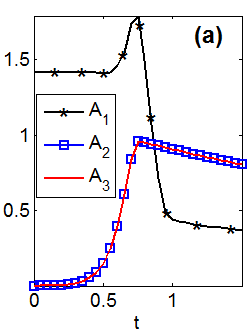
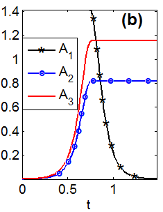
Figure 2: (Color online) Amplitudes $A_{k}=\max_{x\in\Gamma_{k}}|\psi_{k}(t,x)|$ for (1) on the metric graph $\Gamma$ with bond lengths $15$. Initial soliton of the form (4) with $\eta,c=1,10$ and $\xi_{0}=-7.5$, see also (19). (a) Kirchhoff case, $\alpha=(1,1,1)$, $\beta=(1,1,1)$; (b) ballistic case, $\alpha=(1,1.73,1.22)$, $\beta=(1,3,1.5)$. In (a), the blue line is hidden by the red line.

The vertex boundary conditions given by (2) are one possibility to make the linear part of (1) skew-adjoint. The problem (P₀) conserves the norm $N$ and the Hamiltonian $H$ given by

$$N{=}\sqrt{N_{1}^{2}+N_{2}^{2}+N_{3}^{2}},\quad N_{k}^{2}(t){=}\int_{\Gamma_{k}}|\psi_{k}(t,x)|^{2}{\rm d}\xi,$$ (5)

$$H=H_{1}+H_{2}+H_{3},$$

$$\quad H_{k}(t)=\int_{\Gamma_{k}}|{\partial}_{\xi}\psi_{k}(t,\xi)|^{2}-\frac{\beta_{k}}{2}|\psi_{k}(t,x)|^{4}{\rm d}\xi.$$ (6)

It is a question of normalization to set

$$\alpha_{1}=\beta_{1}=1,$$ (7)

which leaves 4 parameters for (P₀), and, of course, the choice of the initial conditions.

Our goal is to compare exact and numerical solutions $(\psi_{1},\psi_{2},\psi_{3})$ of (P₀) with the numerical solutions $\phi=\phi(t,x)$ of an associated NLSE on a fat graph presented in Fig. 1, i.e.,

$${\partial}_{t}\phi={\rm i}(\Delta\phi+\tilde{\beta}(x)|\phi|^{2}\phi),$$ (8)

where $\Delta={\partial}_{x_{1}}^{2}+{\partial}_{x_{2}}^{2},\ x=(x_{1},x_{2})\in\Omega_{\varepsilon}$, and $\Omega_{\varepsilon}=V_{\varepsilon}\cup B_{1,\varepsilon}\cup B_{2,\varepsilon}\cup B_{3,\varepsilon}$ consists of a “vertex–region” $V_{\varepsilon}$ of diameter ${\cal O}(\varepsilon)$, and ${\cal O}(\varepsilon)$-tubes $B_{k}$ around $\Gamma_{k}$, see Fig. 1. In the following Eq.(8) will be called the problem (P_ε). We also use the notation $\phi_{k}$ for $\phi|_{B_{k}}$.

It is clear that different versions of $\Omega_{\varepsilon}$ are possible. Here we choose to give the following 5 parameters to $\Omega_{\varepsilon}$ not a priori present in Eq.(1):

1. the angles $\theta_{2},\theta_{3}$ between the bonds $B_{2}$ and $B_{3}$ and the $x_{1}$–axis,

2. the widths $w_{1},w_{2},w_{3}$ of the different bonds.

In the numerical calculations we impose homogeneous Dirichlet boundary conditions (DBC) for both, (P₀) and (P_ε), at the “ends” of bonds, and for (P_ε) homogeneous Neumann boundary conditions (NBC) ${\partial}_{n}\psi=0$ everywhere else. As our simulations will run on time–scales where the solitons will be well separated from the ends of the bonds, we could as well pose NBC there. Also note that strictly speaking (4) is not a solution over the finite graph, but it is exponentially small at the ends of the bonds.

We take $\tilde{\beta}(x)$ constant on bond $k$ and with suitable jumps near $0$. Furthermore, we set

$$\varepsilon:=w_{1} w_{2}=\delta_{2}\varepsilon w_{3}=\delta_{3}\varepsilon$$,  and (9)

and write $\Omega_{\varepsilon}$ for fixed $\delta_{k},\theta_{k}$, $k=2,3.$ For definiteness we choose

$$B_{1}=\Omega_{\varepsilon}\cap\{x_{1}<0\},\quad B_{2}=\Omega_{\varepsilon}\cap\{x_{2}>w_{1}/2\},$$

$$\quad B_{3}=\Omega_{\varepsilon}\cap\{x_{2}<-w_{1}/2\},$$ (10)

and thus $V_{\varepsilon}=\Omega_{\varepsilon}\setminus(B_{1}\cup B_{2}\cup B_{3})$. Motivated by $\frac{1}{\varepsilon}\int_{\Omega_{\varepsilon}}1{\rm d}x\rightarrow l_{1}+\delta_{2}l_{2}+\delta_{3}l_{3}$ as $\varepsilon\rightarrow 0$, corresponding to $N$ on $\Gamma$ we define the scaled norms

$$N_{\varepsilon}(t)=\left(\frac{1}{\varepsilon}\int_{\Omega_{\varepsilon}}|\phi(t,x)|^{2}{\rm d}x\right)^{1/2},$$ (11)

$$\text{ and }N_{k,\varepsilon}(t):=\left(\frac{1}{\varepsilon}\int_{B_{k}}|\phi(t,x)|^{2}{\rm d}x\right)^{1/2}.$$ (12)

Then $N_{\varepsilon}$ is conserved for (8), and the $N_{k,\varepsilon}$ indicate how much “mass” is in the different bonds.

For the linear problem it is known, Exner and Post (2009), that under the scaling

$$\frac{w_{1}}{w_{k}}=\alpha_{k}^{2},\text{ i.e. }\delta_{k}=\frac{1}{\alpha_{k}^{2}},\text{ and }\psi_{k}=\frac{1}{\alpha_{k}}\phi_{k}|_{\Gamma_{k}},$$ (13)

the vertex conditions (2) appear in the limit $\varepsilon\rightarrow 0$. Then, at least formally, we can expect (P₀) as a “limit” of (P_ε) if

$$\tilde{\beta}|_{B_{k}}=w_{k}\beta_{k}=\alpha_{k}^{-2}\beta_{k}.$$ (14)

If $\alpha_{2}\neq 1$ (or $\alpha_{3}\neq 1$), then the boundary conditions (2) gives jumps from $\psi_{1}$ to $\psi_{2}$ (resp. $\psi_{3}$) at the vertex. This, however, is merely a question of scaling. For instance, setting $\tilde{\psi}_{k}=\alpha_{k}\psi_{k}$ (cf. (13)), we obtain

$${\partial}_{t}\tilde{\psi}_{k} ={\rm i}(\tilde{\psi}_{k}^{\prime\prime}+\gamma_{k}|\tilde{\psi}_{k}|^{2}\tilde{\psi}_{k}),\quad\tilde{\psi}_{1}=\tilde{\psi}_{2}=\tilde{\psi}_{3},$$

$$\quad\tilde{\psi}^{\prime}_{1}=\frac{1}{\alpha_{2}^{2}}\tilde{\psi}_{2}^{\prime}+\frac{1}{\alpha_{3}^{2}}\tilde{\psi}_{3}^{\prime},\text{ at $x=0$},$$ (15)

i.e., continuity at the vertex, where $\gamma_{k}=\beta_{k}\alpha_{k}^{-2}$, as in (14). The scaling given by Eqs.(1),(2) is more custom Sobirov et al. (2010); Exner and Post (2009) than (15), and therefore we stick to (1),(2) as the “limit problem”. Note that the angles $\theta_{1,2}$ of the fat graph do not appear in (P₀).

We expect that for $\varepsilon\rightarrow 0$ solutions $\phi_{k}$ of (P_ε) behave like $\frac{1}{\alpha_{k}}\psi_{k}$ with $\psi_{k}$ being the solutions of (P₀), i.e., are constant in transverse direction on each bond $B_{k}$, with width $w_{k}=\delta_{k}\varepsilon$. Therefore, from Eqs. (12) and (13) we expect

$$N_{k,\varepsilon}^{2}(t)=\frac{1}{\varepsilon}\int_{B_{k}}|\phi_{k}(t,x)|^{2}{\rm d}x\approx\delta_{k}\int_{\Gamma_{k}}|\phi_{k}|_{\Gamma_{k}}|^{2}{\rm d}\xi_{k}$$

$$\approx\delta_{k}\int_{\Gamma_{k}}|\alpha_{k}|^{2}|\psi_{k}|^{2}{\rm d}\xi_{k}=N_{k}^{2}(t),$$ (16)

In the numerical calculations, in addition to $N_{k,\varepsilon}$ we explore the following functions (dropping the dependence on parameters $\varepsilon,\delta_{2,3},\theta_{2,3},c$ and $\eta$):

$$A_{k}(t)= \frac{1}{\alpha_{k}}\max_{x\in B_{k}}|\phi_{k}(t,x)|\quad\text{(scaled amplitude),}$$ (17)

$$m_{k}(t)= \max_{x\in B_{k}}\bigl{|}|\tilde{\psi}_{k}(t,x)|-\frac{1}{\alpha_{k}}|\phi_{k}(t,x)|\bigr{|}$$ (18)

(maximal amplitude distance between (P_ε) and (P₀)).

Here $\tilde{\psi}_{k}$ is the extension of $\psi_{k}$ to $B_{k}$, constant in transverse direction, and for $\psi_{k}$ we either use the explicit formula (4) if (3) holds, or numerics for (P₀) if not. Note that (18) ignores phase differences between $\tilde{\psi}_{k}$ and $\phi_{k}$, as these are less important from the viewpoint of applications.

III Soliton transport in fat graphs

The main practically important problem in the context of wave propagation in branched systems is energy and information transport via solitary waves. The dependence of the soliton dynamics on the topology of a network makes such systems attractive from the viewpoint of tunable transport in low dimensional optical, thermal and electronic devices. Therefore, the treatment of the problems (P₀) and (P_ε) from the viewpoint of vertex soliton transmission is of importance. Our main purpose is to compare propagation of solitons in $\Omega_{\varepsilon}$ with that in $\Gamma$ in particular we are interested to study the “lift” the earlier results Sobirov et al. (2010) from $\Gamma$ to $\Omega_{\varepsilon}$. Transition from two- to one-dimensional wave motion in the shrinking limit is of special importance for this analysis.

In a typical simulation, for (P₀) we use soliton-type initial condition given as

$$\psi_{1}(0,\xi_{1})=\sqrt{2}\eta\,{\rm sech}(\eta(\xi_{1}-x_{0})){\rm e}^{-{\rm i}c\xi_{1}/2},\quad\psi_{2,3}(0,\cdot)\equiv 0$$ (19)

where $x_{0}$ and $\eta$ are chosen in such a way that $\psi_{1}(0,0)$ is very close to $0$. Similarly, for (P_ε) we choose

$$\phi(0,x){=}\left\{\begin{array}[]{ll}\sqrt{2}\,\eta{\rm sech}(\eta(x_{1}{-}x_{0})){\rm e}^{-{\rm i}cx_{1}/2}&\ x_{1}<0,\\ 0&\ \text{else},\end{array}\right.$$ (22)

i.e., we extend the initial conditions (19) trivially in transverse direction. We then run both, (P₀) and (P_ε) until some final time $t_{1}$ such that the solitons launched by (19) and (22), respectively, have interacted with the vertex, and have been reflected or transmitted sufficiently far into the bonds (see the appendix for the numerical methods used). Our main solution diagnostics will be the time dependent norms $N_{k}(t),N_{k,\varepsilon}(t)$, the amplitudes $A_{k}(t),A_{k,\varepsilon}(t)$, the distances $m_{k}(t)$, and the reflection coefficients defined below.

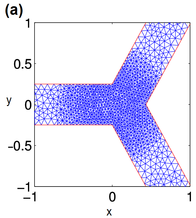
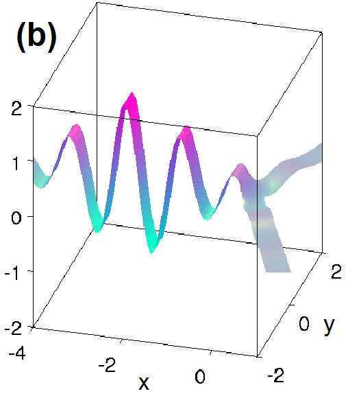
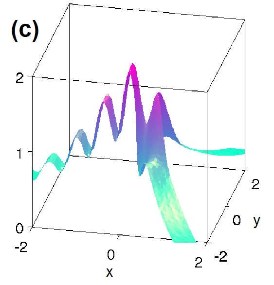
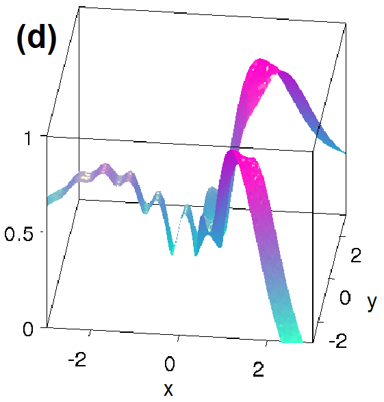
Figure 3: (Color online) Numerical solution of (P_ε) for $\delta_{2,3}=1$ and $\varepsilon=0.5$, i.e. $w=(0.5,0.5,0.5)$; $\tilde{\beta}\equiv 1$, $l=(15,15,15)$, $\theta=(\pi/3,\pi/3)$. Initial condition (22) with $x_{0}=-l/2$ and $\eta,c=1,10$. (a) Geometry and mesh near the vertex. (b) ${\rm Re}\psi(0.5,\cdot)$ real part of incoming soliton at $t=0.5$; (c),(d) $|\psi(\cdot,x)|$ during and after transmission/reflection trough/at the vertex.

For definiteness, we consider $\Gamma_{1}$ as the “incoming” bond and $\Gamma_{2,3}$ as “outgoing” ones. In Fig. 3 solutions of the problem (P_ε) for the Kirchhoff boundary conditions are presented for the case of a “relatively fat” graph ($\varepsilon=0.5$), while Fig. 4 shows the plots of the corresponding norms $N_{k}$ and amplitudes $A_{k}$ for the simulation for (P_ε) in Fig. 3 (Kirchhoff case), together with the respective quantities for (P₀). At this relatively large $\varepsilon=0.5$ there is a significant difference between (P_ε) and (P₀).

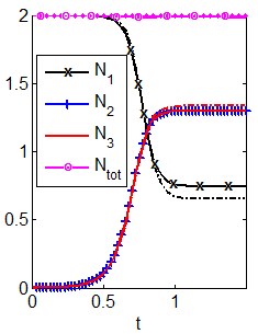
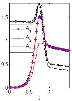
Figure 4: (Color online) Norms and amplitudes corresponding to the solutions presented in Fig.3. Dashed lines present respective quantities from (P₀); the blue lines are all hidden by the red lines.

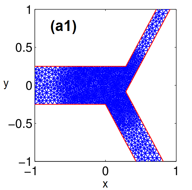
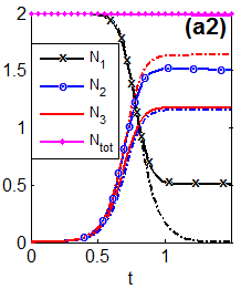
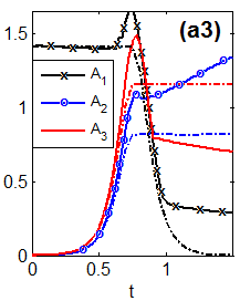
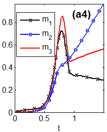
Figure 5: (Color online) Norms and amplitudes for fat and metric graphs with $1/\alpha_{2}^{2}+1/\alpha_{3}^{2}=1$ and $\beta_{k}=\alpha_{k}^{2}$, hence $\tilde{\beta}=1$, and plots of the amplitude distances $m_{k,\varepsilon}$, cf. (18). Here $\theta_{1}=\theta_{2}=\pi/3$, $\delta_{2}=1/3,\delta_{3}=2/3$, and $\varepsilon=0.5$, hence $w=(0.5,0.33,0.17)$.(see Fig. 6). In (a1) we also plot the geometry and mesh near the vertex. For the lengths of the bonds we again have $l_{1}=l_{2}=l_{3}=15$. In (a2),(a3) the full lines are $N_{\varepsilon,k}$ and $\frac{1}{\alpha_{k}}A_{\varepsilon,k}$, respectively, and the dashed lines are $N_{k}$ and $A_{k}$, cf. Fig. 2(b), and similarly in (b1),(b2) and (c1),(c2).

In the following we focus on soliton reflection and transmission in the shrinking limit, $\varepsilon\to 0$ for the ”ballistic” boundary conditions given by (3) on (P₀). In Fig.5 and 6 we plot the diagnostics defined above for different $\varepsilon$ on an otherwise fixed graph fulfilling (3), i.e., for the ballistic case. As $\varepsilon\rightarrow 0$, the amplitudes and masses in the different bonds get close to the metric graph case, and also the (numerical) wave functions as a whole converge to the ones on the metric graph, with one small qualification: While the main mismatches between (P_ε) and (P₀) result from reflection and position shifts of the incoming soliton during interaction with the vertex around $t=7.5$, already for $0<t<5$, i.e., before interaction of the soliton with the vertex, there is a small linear growth of $m_{1,\varepsilon}$, i.e., of the amplitude mismatch in the incoming bond. This is not a property of the fat graph itself, but related to the fact that it is difficult to accurately resolve the speed of the soliton numerically. In other words, for small $\varepsilon$, a significant part of mismatch between our (numerical) fat graph solution $\phi$ and the (analytical) metric graph solution $(\psi_{1},\psi_{2},\psi_{3})$ from Sobirov et al. (2010) is not due to the behaviour at the vertex, but due to an error in (numerical) soliton speed, which results in a position mismatch growing in time (see the Appendix for further discussion). However, noting the different scales in panels (a4),(b3) and (c3) strongly indicates the convergence of the (P_ε) wave function to the (P₀) wave function in $L^{\infty}$ (modulo phases), uniformly on bounded time intervals.

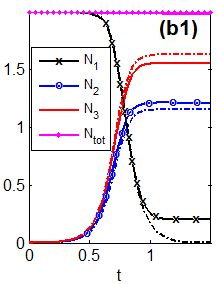
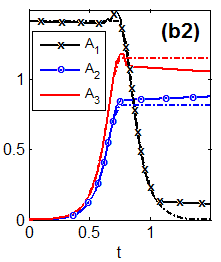
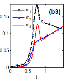
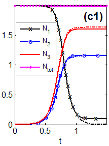
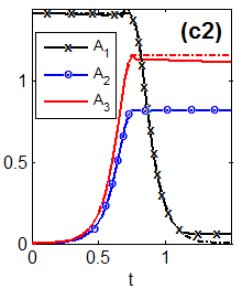
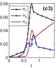
Figure 6: (Color online) Continuation of Fig.5, $\varepsilon=0.2$ in (b) and $\varepsilon=0.1$ in (c)

From the viewpoint of practical applications, probably the most important question is how much of an incoming soliton is reflected resp. transmitted in the vertex region of a fat graph. To display this in a concise way, for (P_ε) we define the reflection and transmission coefficients

$$r_{k,\varepsilon}^{A} :=A_{k,\varepsilon}(t_{1})/A_{1,\varepsilon}(0)\quad\text{(amplitude reflection)},$$ (23)

$$r_{k,\varepsilon}^{N} :=N_{k,\varepsilon}(t_{1})/N_{1,\varepsilon}(0)\quad\text{(mass reflection)},$$ (24)

where again we dropped the dependence on parameters $w_{2,3},\beta_{2,3},c$ and $\eta$ here, but will plot $r_{k,\varepsilon}^{A},r_{k,\varepsilon}^{N}$ as functions of some parameters below. Thus, e.g., $r_{1,\varepsilon}^{A}=0$ (and thus also $r_{1,\varepsilon}^{N}=0$) means zero reflection of an incoming soliton at the vertex, while, e.g., $r_{2,\varepsilon}^{N}=1$ means that all of the “mass” was transmitted to bond two. These extreme cases of course do not occur, but the goal is, e.g., to tune $r_{k,\varepsilon}^{N,A}$. The corresponding quantities for (P₀) are defined as

$$r_{k}^{A}:=A_{k}(t_{1})/A_{1}(0),\quad r_{k}^{N}:=N_{k}(t_{1})/N_{1}(0),$$ (25)

and the transmission formula (3) means, that $r_{1}^{A,N}\rightarrow 0$ in the limit of infinite bonds and of $t_{1}\rightarrow\infty$.

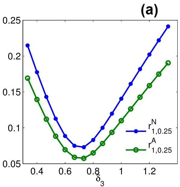
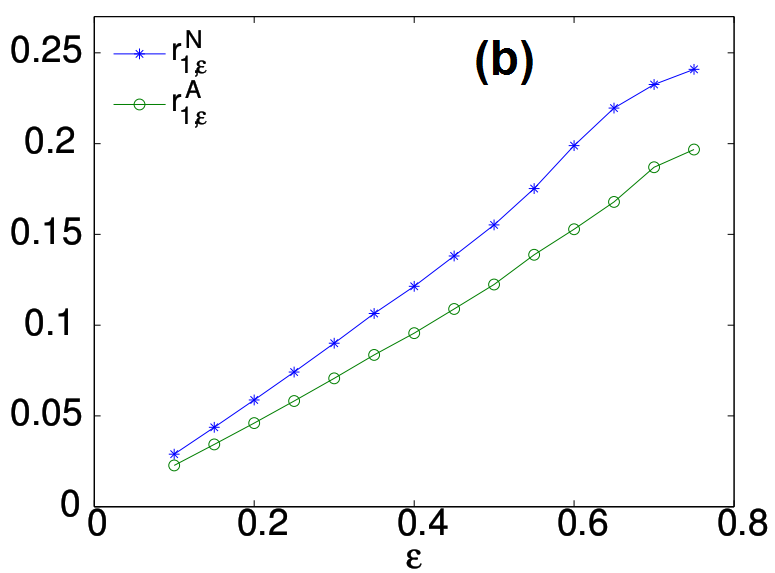
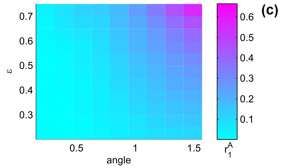
Figure 7: (Color online) (a)$r_{k,\varepsilon}^{N}$ and $r_{k,\varepsilon}^{A}$ as functions of the (relative) thickness $\delta_{3}$ of the third bond, with fixed $\varepsilon=0.25$,$\theta_{1,2}=\pi/4$,$\delta_{1}=1,\delta_{2}=1/3$,$l=(15,15,15)$, and $(\eta,c)=(1,10)$. (b) $r_{k,\varepsilon}^{N}$ and $r_{k,\varepsilon}^{A}$ as functions of $\varepsilon$, with $\delta_{3}=2/3$ (ballistic case) and the remaining parameters fixed as in (a). (c) $r_{1,\varepsilon}^{A}$ as a function of $\varepsilon$ and angles $\theta:=\theta_{1}=\theta_{2}$, remaining parameters as in (b).

Fig.7 presents plots of the reflections as a function of different parameters such as bond thickness, $\varepsilon$, angle between the bonds, $\theta$ and coefficient, $\delta_{3}$. Of course, the ballistic regime is an idealization, and in order to quantify the reflections when we perturb it, in Fig. 7(a) we study the dependence of $r_{k,\varepsilon}^{N}$ and $r_{k,\varepsilon}^{A}$ on the mismatch $\frac{1}{\beta_{1}}-\frac{1}{\beta_{2}}-\frac{1}{\beta}_{3}$. As we have chosen $\beta_{k}=w_{k}^{2}=1/\delta_{k}$, $k=2,3$, in (a) we fix $\delta_{2}=1/3$ and let $\delta_{3}$ vary between $1/3$ and $4/3$, such that again $\delta_{3}=2/3$ corresponds to the minimal reflection case. Clearly, the minima of $r_{k,\varepsilon}^{N}$ and $r_{k,\varepsilon}^{A}$ are attained close to $\delta_{3}=2/3$, and these functions are somewhat steep. Similar graphs were obtained in other geometries (e.g., angles), and thus in applications it appears desireable to move as close as possible to the ballistic case by, e.g., fine tuning the widths of the bonds. In Fig. 7(b) the vertex reflection coefficients (both for norm and amplitude) are plotted as functions of the graph thickness $\varepsilon$ for the case described by (3). The limit $\varepsilon\rightarrow 0$ again shows a rather smooth transition from the “scattering” to ballistic regime.Figure 7(c) presents the dependence of $r_{1,\varepsilon}^{A}$ on the graph thickness and the angles $\theta=\theta_{1}=\theta_{2}$. Even though the angles do not appear in the $\varepsilon\rightarrow 0$ limit (P₀), at finite $\varepsilon$ they of course play an important role. Ballistic transport through the vertex occurs in the shrinking limit as well as in the limit of small angles.

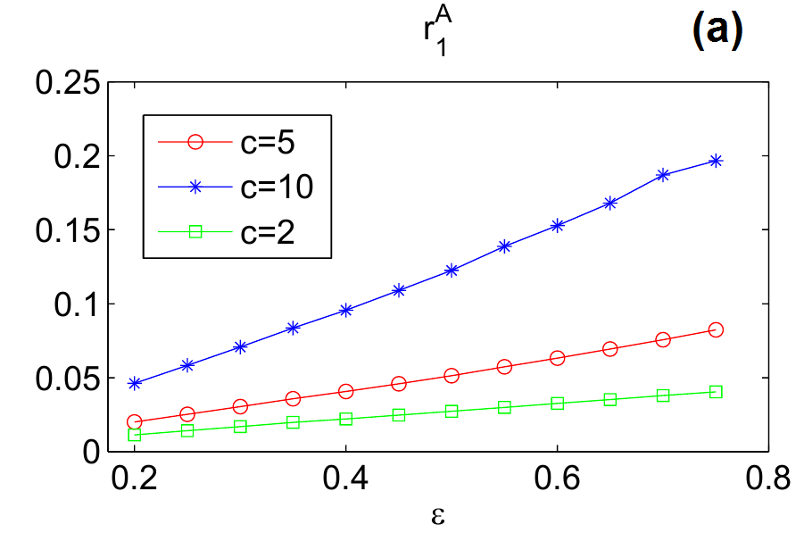
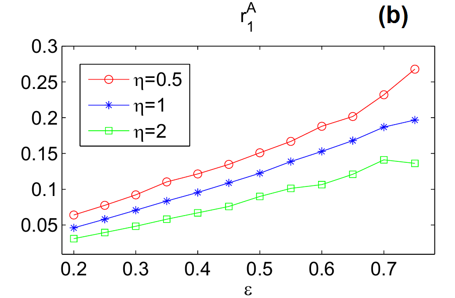
Figure 8: (Color online) Reflection coefficients as functions of thickness $\varepsilon$, with fixed $\theta_{1,2}=\pi/4$, $l=(15,15,15)$ for differrent values of (a) speeds (with fixed $\eta=1$) and (b) amplitudes (with fixed $c=10$) of soliton in the ballistic case.

Besides the equal angle case $\theta_{2}=\theta_{3}$, we checked a variety of other configurations with $\theta_{2}<\theta_{3}$, for various $\theta_{1,2}$ between $\pi/20$ and $\pi/2$. The results remain qualitatively similar to Figs. 5–7, i.e., in the ballistic case the reflection coefficients vanish as $\varepsilon\rightarrow 0$, and as above the (P_ε) wave functions converge to the $\theta_{2,3}$ independent wave functions $(\psi_{1},\alpha_{2}\psi_{2},\alpha_{3}\psi_{3})$ of (P₀). As the convergence for $\varepsilon\rightarrow 0$ is clearly linear, an interesting question is how to choose a first order in $\varepsilon$ correction of the fat graph geometry or NLSE coefficients that minimizes $r_{1,\varepsilon}^{N,A}$ also for finite $\varepsilon>0$.

An important issue for particle and wave transport in fat graphs is the dependence of the scattering on initial soliton velocity and amplitude. In Fig.8 reflection coefficients are plotted as functions of bond thickness $\varepsilon$ for different initial velocities (a) and amplitudes (b). The dependence of reflection on initial data is significant for fat graphs, with, e.g., less reflection for slower and longer waves, as should be expected. However, in the shrinking limit the reflections vanish in all cases considered.

Finally, although in Figs. 5–7 we mainly focused on the ballistic case $\delta_{2}+\delta_{3}=1$, for other values of $\delta_{2},\delta_{3}$, as for instance $\delta_{2}=\delta_{3}=1$ in Fig. 4, as $\varepsilon\rightarrow 0$ we have the same kind of convergence of $(N_{k,\varepsilon},\frac{1}{\alpha_{k}}A_{k,\varepsilon},r_{k,\varepsilon}^{N,A},m_{k,\varepsilon})$ to $(N_{k},A_{k},r_{k}^{N,A},0)$ as above, and altogether of $\phi$ to $(\psi_{1},\alpha_{2}\psi_{2},\alpha_{3}\psi_{3})$, i.e., of (P_ε) to (P₀).

IV Conclusions

We studied soliton transport in tube like networks modeled by the time-dependent NLSE on fat graphs, i.e. graphs with finite bond thickness. We numerically solved the NLSE on fat graphs for different values of thickness, and studied behavior of solutions and vertex reflection coefficients in the shrinking limit. It is found that in the shrinking limit solutions of the NLSE on fat graphs converge to those on the associated metric graphs, and hence the conditions (3) for reflectionless transport also work on fat graphs with small $\varepsilon$. The dependence of the vertex reflection coefficient on the bond thickness and on the angle between the bonds of fat graph is also studied.

At this point it is not clear in which norms we can expect or analytically show convergence of solutions of (P_ε) to solutions of (P₀), as $\varepsilon\rightarrow 0$. First, following Kosugi (2002) this will be discussed for the stationary case, including some potentials at the vertex in order to have nontrivial stationary solutions for the fat graph and the metric graph, cf. Adami et al. (2012); Sabirov et al. (2013). An important point in the study of wave(particle) dynamics in fat graphs is the definition of the fat graph thickness at which one can neglect transverse motion and consider the system as one-dimensional. The above treatment allows us to define such a regime. However, the transition from two- to one dimensional motion is rather smooth and there is no critical value of the bond thickness at which a ”jump” from the fat to the metric graph occurs. In any case, we believe that our numerical results should be considered as a first step in the way for the study of particle and wave transport described by nonlinear evolution equations on fat graphs. In addition, can be useful for further analytical studies of the NLSE on such graphs.

Appendix: Details of the numerical approach

We discretize (P₀) by second order spatial finite differences (FD) and denote $u_{j}{=}u_{j}(t){=}\psi_{1}(t,\xi_{1,j})$, $\xi_{j}{=}-l_{1}+j\delta$, $v_{j}=v_{j}(t)=\psi_{2}(t,\xi_{2,j}),w_{j}=w_{j}(t)=\psi_{3}(t,\xi_{3,j})$, $j{=}1,\ldots,n-1$, such that, e.g., $u_{j}^{\prime\prime}=\frac{1}{\delta^{2}}(u_{j-1}-2u_{j}+u_{j+1})$. Moreover, we set

$$u_{0}=\psi_{1}(-l_{1})=0 v_{n}=\psi_{2}(l_{2})=0 w_{n}=\psi_{3}(l_{3})=0$$, , ,

and $$u_{n}=\psi_{1}(0) v_{0}=\psi_{2}(0) w_{0}=\psi_{3}(0)$$, , and .

The vertex conditions then are $u_{n}{=}\alpha_{2}v_{0}{=}\alpha_{3}w_{0}$, $u_{n}^{\prime}=\frac{1}{\alpha_{2}}v_{0}^{\prime}+\frac{1}{\alpha_{3}}w_{0}^{\prime}.$ Using one-sided FD for $u_{n}^{\prime},v_{0}^{\prime}$ and $w_{0}^{\prime}$ we have

$$u_{n}^{\prime} =\frac{1}{\delta}(u_{n}-u_{n-1})=\frac{1}{\delta}\left(\frac{1}{\alpha_{2}}(v_{1}-v_{0})+\frac{1}{\alpha_{3}}(w_{1}-w_{0})\right),$$

$$\Leftrightarrow u_{n}(1+\frac{1}{\alpha_{2}^{2}}+\frac{1}{\alpha_{3}^{2}})=u_{n-1}+\frac{1}{\alpha_{2}}v_{1}+\frac{1}{\alpha_{3}}w_{1}.$$ (26)

which expresses $u_{n}$ and hence $v_{0},w_{0}$ in terms of $u_{n-1},v_{1},w_{1}$. The resulting $z^{\prime\prime}:=(u_{i}^{\prime\prime},v_{i}^{\prime\prime},w_{i}^{\prime\prime})_{i=1,\ldots,n-1}$ can be best expressed by a matrix vector multiplication $Mz$. The scheme differs from the one in Sobirov et al. (2010), where the PDE is extended up to and including the vertex from the left, which works well to discretize the reflectionsless solutions (4) in case of (3), but it introduces an asymmetry between the bonds not present in (P₀).

To integrate the resulting ODEs ${\partial}_{t}z={\rm i}(Mz+\beta|z|^{2}z)$, where $\beta=(\beta_{u},\beta_{v},\beta_{w})$ with obvious meaning, we use an explicit scheme with stepsize $\tau$ in $t$, namely

$$z^{n+1}=z^{n-1}+2\tau(Mz^{n}+\beta|\tilde{z}^{n}|^{2}z^{n}),$$ (27)

where $\tilde{u}_{i}=\frac{1}{2}(u_{i-1}+u_{i+1})$ and similar for $\tilde{v}_{i}$ and $\tilde{w}_{i}$. For $\tau\leq\delta^{2}/4$ this conserves $N(t)$ with high accuracy, and also $H(t)$.

To simulate (P_ε) we write it as a 2-component real system for $z=(u,v)$ where $\psi=u+{\rm i}v$. We set up and discretize the domain $\Omega_{\varepsilon}$ using routines from pde2path Uecker et al. (2014) which are based on the FEM from the Matlab pdetoolbox. For efficiency it is quite useful to apply some local mesh refinement near the vertex. We typically work with meshes of 5000-20000 triangles, requiring a maximal mesh size of $\varepsilon/6$ before local refinement. Eq. (8) then translates into the system of ODEs

$$Mz_{t}=Kz+F(z)$$ (28)

where $M$ is the mass matrix, $K=K_{{\rm i}\Delta}$ is the stiffness matrix, and $F(z)$ is the FEM nonlinearity. For the time integration of (28) we use a semilinear trapez rule, i.e., setting $z_{n}=z(\cdot,t_{n}),t_{n}=n\tau$, with typically $\tau\approx 10^{-4}$ to $10^{-3}$,

$$[M-\frac{\tau}{2}K]z^{n+1}=[M+\frac{\tau}{2}K]z^{n}+\tau F(z^{n}).$$ (29)

Over relevant time-scales (29) conserves (the discretized version of) $N_{\varepsilon}$ from (12) reasonably well, see, e.g., Fig. 4, 5(a2), and 6(b1), (c1), but, as already indicated, dependent on the discretizations there are some slightly more significant errors in the numerical soliton speed. To quantify this, we used (29) to propagate a soliton of amplitude and speed $(\eta,c)=(1,10)$ on a straight bond $x_{1}\in(-30,0)$ from $(t,x_{1,s})=(0,-20)$ to position $x_{1,e}\approx-10$ at $t=1$ for various time steps $\tau$ and mesh-sizes $h$, and calculated the error

$$e(\tau,h):=\max_{x}|\,|\tilde{\phi}(1,x)|-|\phi(1,x)|\,|,$$

where $\tilde{\phi}$ and $\phi$ denote the numerical and the exact solution, respectively. In reasonable $\tau,h$ ranges $e(\tau,h)$ turns out to be roughly a linear function of $\tau,h$. See Fig. 9(a) for $e(\cdot,0.04)$ as an example, while (b) shows $|\tilde{\phi}(1,x)|-|\phi(1,x)|$ for $\tau=10^{-4}$ and thus illustrates that (29) propagates the soliton too quickly.

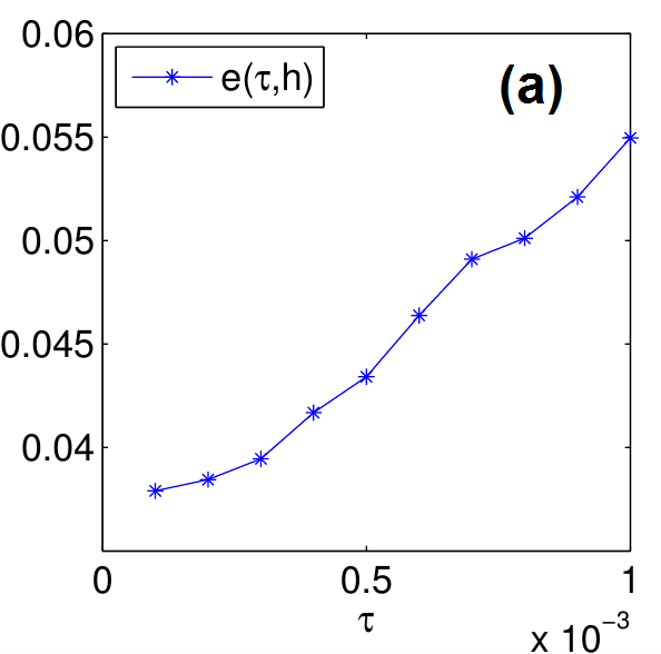
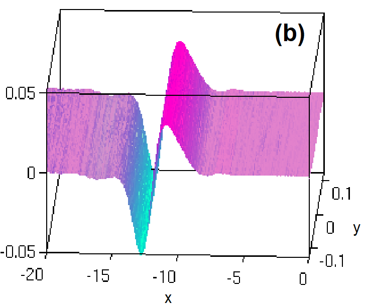
Figure 9: Numerical error of the scheme 29 over a straight bond.(a) error dependence on $\tau$; (b) $|\tilde{\phi}(1,\cdot)|{-}|\phi(1,\cdot)|$, $\tau{=}10^{-4}$.

We also tried the relaxation scheme from Besse (2004) which conserves $N_{\varepsilon}$ slightly better, but becomes computationally much slower, mainly since one can no longer $LU$-pre-factorize $M-\frac{\tau}{2}K$. On the other hand, the stability requirements for explicit schemes like (27) become prohibitive for fine meshes near the vertex. For (29), typical computation times for the propagation of a solitary wave through the network are on the order of 1 minute.

References

- Sobirov et al. (2010) Z. Sobirov, D. Matrasulov, K. Sabirov, S. Sawada, and K. Nakamura, Phys. Rev. E 81, 066602 (2010).
- Cascaval and Hunter (2010) R. Cascaval and C. Hunter, Libertas Math. 30, 85-98 (2010).
- Banica and Ignat (2011) V. Banica and L. Ignat, J. Math. Phys. 52, 083703 (2011).
- Adami et al. (2011) R. Adami, C. Cacciapuoti, D. Finco, and D. Noja, Rev. Math. Phys. 23, 409 (2011).
- Adami et al. (2012) R. Adami, C. Cacciapuoti, D. Finco, and D. Noja, Europhys. Letters (2012).
- Adami et al. (2012) R. Adami, C. Cacciapuoti, D. Finco, and D. Noja, J. Phys. A: Math. Theor. 45, 192001 (2012).
- Adami et al. (2013) R. Adami, D. Noja, and C. Ortoleva, J.Math. Phys. 54, 013501 (2013).
- Noja (2014) D. Noja, Phil. Trans. R. Soc. A 372 (2014).
- Gnutzmann et al. (2011) S. Gnutzmann, U. Smilansky, and S. Derevyanko, Phys. Rev. A 83, 033831 (2011).
- Sabirov et al. (2013) K. Sabirov, Z. Sobirov, D. Babajanov, and D. Matrasulov, Phys. Letters A 377, 860865 (2013).
- Leboeuf and Pavloff (2001) P. Leboeuf and N. Pavloff, Phys. Rev. A 64, 033602 (2001).
- Paul et al. (2007) T. Paul, M. Hartung, K. Richter, and P. Schlagheck, Phys. Rev. A p. 063605 (2007).
- de Oliveira et al. (2010) I. N. de Oliveira, F. A. B. F. de Moura, M. L. Lyra, J. S. Andrade, Jr., and E. L. Albuquerque, Phys. Rev. E 81, 030104(R) (2010).
- Yomosa (1983) S. Yomosa, Phys. Rev. A 27, 2120 (1983).
- Yakushevich et al. (2002) L. V. Yakushevich, A. V. Savin, and L. I. Manevitch, Phys. Rev. E 66, 016614 (2002).
- Burioni et al. (2006) R. Burioni, D. Cassi, P. Sodano, A. Trombettoni, and A. Vezzani, Phys. Rev. E 73, 066624 (2006).
- Markowsky and Schopohl (2014) A. Markowsky and N. Schopohl, Phys. Rev. A 89, 013622 (2014).
- Demidov et al. (2009) V. E. Demidov, J. Jersch, S. O. Demokritov, K. Rott, P. Krzysteczko, and G. Reiss, Phys. Rev. B 79, 054417 (2009).
- Biggs (2012) N. R. Biggs, Wave Motion 49, 24–33 (2012).
- Rubinstein and Schatzman (2001) J. Rubinstein and M. Schatzman, Arch. Rat. Mech. Anal. 160, 271 (2001).
- Kuchment and Zeng (2001) P. Kuchment and H. Zeng, J. Math. Anal. and Appl. 258, 671 (2001).
- Exner and Post (2005) P. Exner and O. Post, J. Geom. Phys. 54, 77 (2005).
- Post (2006) O. Post, Ann. Henri Poincaré 7, 933 (2006).
- Exner and Post (2007) P. Exner and O. Post, J. Math. Phys. 48, 092104+43 (2007).
- Exner and Post (2009) P. Exner and O. Post, J. Phys. A, Math. Theor. 42, 22 (2009).
- Exner (2011) P. Exner, in Mathematics in science and technology. Mathematical methods, models and algorithms in science and technology. Proceedings of the satellite conference of the ICM 2010, New Delhi, India, August 14–17, 2010. (2011), pp. 71–92.
- Exner and Post (2013) P. Exner and O. Post, Commun. Math. Phys. 322, 207 (2013).
- Cacciapuoti and Exner (2007) C. Cacciapuoti and P. Exner, J. Phys. A 40, F511 (2007).
- Post (2012) O. Post, Spectral analysis on graph-like spaces. (Berlin: Springer, 2012).
- Ruedenberg and Scherr (1953) K. Ruedenberg and C. W. Scherr, J. Chem. Phys. 21, 1565 (1953).
- Molchanov and Vainberg (2007) S. Molchanov and B. Vainberg, Commun. Math. Phys. 273, 533 (2007).
- Molchanov and Vainberg (2010) S. Molchanov and B. Vainberg, in Integral methods in science and engineering. IMSE 2008, Santander, Spain (Basel: Birkhäuser, 2010), pp. 255–278.
- Dell’Antonio and Costa (2010) G. Dell’Antonio and E. Costa, J. Phys. A, Math. Theor. 43, 23 (2010).
- Kosugi (2002) S. Kosugi, Journal of Differential Equations 183, 165 (2002).
- Grieser (2008a) D. Grieser, Proc. Lond. Math. Soc. 97, 718 (2008a).
- Mehran (1978) R. Mehran, IEEE Transactions on Microwave Theory and Techniques 26, 4005 (1978).
- Exner et al. (1988) P. Exner, P. Seba, and P. Stovicek, J. Phys. A 21, 4009 (1988).
- Exner and Seba (1989) P. Exner and P. Seba, Rep. Math. Phys. 28, 7 (1989).
- Kostrykin and Schrader (1999) V. Kostrykin and R. Schrader, Rev. Math. Phys. 11, 187 (1999).
- Kottos and Smilansky (1999) T. Kottos and U. Smilansky, Ann. Phys. 274, 76 (1999).
- Gnutzmann and Smilansky (2006) S. Gnutzmann and U. Smilansky, Adv. Phys. 55, 527 (2006).
- Gnutzmann et al. (2010) S. Gnutzmann, J. Keating, and F. Piotet, Ann. Phys. 325, 2595–2640 (2010).
- Grieser (2008b) D. Grieser, in Analysis on graphs and its applications. Isaac Newton Institute, Cambridge, UK, January 8–June 29, 2007 (AMS, 2008b), pp. 565–593.
- Raugel (1995) G. Raugel, in Dynamical systems (Montecatini Terme, 1994) (Springer, Berlin, 1995), vol. 1609 of Lecture Notes in Math., pp. 208–315.
- Uecker et al. (2014) H. Uecker, D. Wetzel, and J. Rademacher, Numerical Mathematics: Theory Methods Applications 7, 58-106 (2014).
- Besse (2004) C. Besse, SIAM J. Num. Anal. 42, 934 (2004).