On the spherically-symmetric turbulent accretion

Abstract

We analize the quasi-spherical accretion in the presence of axisymmetric vortex turbulence. It is shown that in this case the turbulence changes mainly the effective gravity potential but not the effective pressure.

1 Introduction

An activity of many astrophysical sources (Active Galactic Nuclei, Young Stellar Objects, Galactic X-ray sources, microquasars) is associated with the accretion. For this reason, the accretion onto compact objects (neutron stars or black holes) is the classical problem of modern astrophysics (see, e.g., Shapiro & Teukolsky (1983); Lipunov (1992) and references therein). At present the analytical approach, whose foundation was laid back in the mid-twentieth century (Bondi & Hoyle, 1944; Bondi, 1952), began to be supplanted by numerical simulations (Hunt, 1979; Petrich et al, 1989; Ruffert & Arnett, 1994; Toropin et al., 1999; Toropina et al., 2012). Analytical solutions were found only in exceptional cases (Bisnovatyi-Kogan et al, 1979; Petrich et al, 1988; Anderson, 1989; Beskin & Pidoprygora, 1995; Beskin & Malyshkin, 1996; Pariev, 1996).

It should be emphasized that last time the focus of the research has been shifted to numerical magnetohydrodynamic simulations, within which framework it has become possible to take into account the turbulent processes associated with magnetic reconnection, magnetorotational instability, etc. (Balbus & Hawley, 1989; Brandenburg & Sokoloff, 2002; Krolik & Hawley, 1979). However, in our opinion, some important features of the turbulent accretion can still be understood on the ground of simple analytical model.

The problem of turbulent accretion and stellar wind has been discussed in various papers. Axford & Newman (1967) showed that the inclusion of viscosity and heat conduction allows to remove singularity at the sonic surface and leads to the appearance of weak non-Rankine-Hugoniot shock waves in the solutions. Kovalenko & Eremin (1998) examined the spatial stability of spherical adiabatic Bondi accretion on to a point gravitating mass against external vortex perturbations. Bhattacherjee & Ray (2005) also discussed the role of turbulence in a spherically symmetric accreting system. In their paper it was shown that the sonic horizon of the transonic inflow solution is shifted inwards, in comparison with inviscid flow, as a consequence of dynamical scaling for sound propogation in accretion process. Shcherbakov (2008) formulated a model of spherically symmetric accretion flow in the presence of magnetohydrodynamic turbulence.

In this paper we show on the ground of the simple model how the turbulence affects the structure of the spherically symmetric accretion. In the first part, we formulate the basic equations of ideal steady-state axisymmetric hydrodynamics, which are known to be reduced to one second-order equation for the stream function. Then, in the second part, the structure of the solitary curl is discussed in detail. Finally, in the third part we consider two toy models describing axisymmetric turbulence. It is shown that the turbulence changes mainly the effective gravity potential but not the effective pressure.

2 Basic equations

First of all, let us formulate basic hydrodynamical equations describing axisymmetric stationary flows. Then, as is well-known, it is convenient to introduce the potential $\Phi(r,\theta)$ connected with the poloidal velocity ${\bf v}_{\rm p}$ and the number density $n$ as (Heyvaerts, 1996; Beskin, 2010)

$$n{\bf v}_{\rm p}=\frac{\nabla\Phi\times{\bf e}_{\varphi}}{2\pi r\sin\theta}.$$ (1)

This definition results in the following properties

• The continuity equation $\nabla\cdot(n{\bf v})=0$ is satisfied automatically.

• It is easy to verify that ${\rm d}\Phi=n{\bf v}\cdot{\rm d}{\bf S}$, where ${\rm d}{\bf S}$ is an area element. As seen, the potential $\Phi(r,\theta)$ is a particle flux through the circle $r,\theta,0<\varphi<2\pi$. In particular, the total flux through the surface of the sphere of radius $r$ is $\Phi_{\rm tot}=\Phi(r,\pi)$.

• As ${\bf v}\cdot\nabla\Phi=0$, the velocity vectors ${\bf v}$ are located on the surfaces $\Phi(r,\theta)=$ const.

In this case, three conservation laws for energy $E_{\rm n}$, angular momentum $L_{\rm n}$, and the entropy $s$ can be formulated as

$$E_{\rm n} = E_{\rm n}(\Phi)=\frac{{v}^{2}}{2}+{w}+\varphi_{\rm g},$$ (2)

$$L_{\rm n} = L_{\rm n}(\Phi)={v}_{\varphi}r\sin\theta,$$ (3)

$$s = s(\Phi).$$ (4)

Here $w$ is the specific enthalpy, and $\varphi_{\rm g}$ is the gravitational potential.

In what follows we for simplicity consider the entropy $s(\Phi)$ to be constant. Then the equation for the stream function $\Phi(r,\theta)$ (which is no more than the projection of the Euler equation onto the axis perpendicular to the velocity vector ${\bf v}$) looks like (cf. Heyvaerts (1996))

$$\varpi^{2}\nabla_{k}\left(\frac{1}{\varpi^{2}n}\nabla^{k}\Phi\right)+4\pi^{2}nL_{\rm n}\frac{{\rm d}L_{\rm n}}{{\rm d}\Phi}-4\pi^{2}\varpi^{2}n\frac{{\rm d}E_{\rm n}}{{\rm d}\Phi}=0,$$ (5)

where $\varpi=r\sin\theta$. This equation represents the balance of forces in a normal direction to flow lines. In partucular, for spherically symmetric flow, i.e., for $E_{\rm n}(\Phi)=$ const, $L_{\rm n}(\Phi)=0$, it has the solution

$$\Phi=\Phi_{0}(1-\mathrm{cos}~{}\theta).$$ (6)

In the following, we deal with the linear angular operator

$$\hat{\cal L}_{\theta}=\sin\theta\frac{\partial}{\partial\theta}\left(\frac{1}{\sin\theta}\frac{\partial}{\partial\theta}\right),$$ (7)

originated from Eqn. (5). It has eigenfunctions

$$Q_{0}=1-\mathrm{cos}~{}\theta,$$ (8)

$$Q_{1}=\sin^{2}\theta,$$ (9)

$$Q_{2}=\sin^{2}\theta~{}\mathrm{cos}~{}\theta,$$ (10)

$$\dots$$

$$Q_{m}=\frac{2^{m}m!(m-1)!}{(2m)!}\sin^{2}\theta~{}{\cal P}_{m}^{\prime}(\mathrm{cos}~{}\theta),$$ (11)

and the eigenvalues

$$q_{m}=-m(m+1).$$ (12)

Here ${\cal P}_{m}(x)$ are the Legendre polynomials and the dash indicates their derivatives.

Let us consider now the small disturbance of the spherically symmetric flow, so that one can write down the flux function as

$$\Phi=\Phi_{0}[1-\mathrm{cos}~{}\theta+\varepsilon^{2}f(r,\theta)]$$ (13)

with the small parameter $\varepsilon\ll 1$. Then Eqn. (5) can be linearised, while the equation for the perturbation function $f(r,\theta)$ is written as (Beskin, 2010):

$$-\varepsilon^{2}D\frac{\partial^{2}f}{\partial r^{2}}-\frac{\varepsilon^{2}}{r^{2}}(D+1)\sin\theta\frac{\partial}{\partial\theta}(\frac{1}{\sin\theta}\frac{\partial f}{\partial\theta})+\varepsilon^{2}N_{r}\frac{\partial f}{\partial r}=$$ (14)

$$=-\frac{4\pi^{2}n^{2}r^{2}}{\Phi_{0}^{2}}\sin\theta(D+1)\frac{{\rm d}E_{\rm n}}{{\rm d}\theta}$$

$$+\frac{4\pi^{2}n^{2}}{\Phi_{0}^{2}}(D+1)\frac{L_{\rm n}}{\sin\theta}\frac{dL_{\rm n}}{d\theta}-\frac{4\pi^{2}n^{2}}{\Phi_{0}^{2}}\frac{\mathrm{cos}\theta}{\sin^{2}\theta}L_{\rm n}^{2}.$$

Here $D=-1+c_{\rm s}^{2}/v^{2}$, and $N_{r}=2/r-4\pi^{2}n^{2}r^{2}GM/\Phi_{0}^{2}$.

This equation allows us to seek the solution in the form

$$f(r,\theta)=\sum_{m=0}^{\infty}g_{m}(r)Q_{m}(\theta).$$ (15)

Introducing now dimensionless variables

$$x=\frac{r}{r_{*}},\,u=\frac{n}{n_{*}},\,l=\frac{c_{\rm s}^{2}}{c_{*}^{2}},$$ (16)

where the $*$-values correspond to the sonic surface (which can be taken from the zero approximation), we can write the ordinary differential equations describing the radial functions $g_{m}(r)$:

$$(1-x^{4}lu^{2})g^{\prime\prime}_{m}+2\left(\frac{1}{x}-x^{2}u^{2}\right)g^{\prime}_{m}+m(m+1)x^{2}lu^{2}g_{m}=$$ (17)

$$=k_{m}\frac{R^{2}}{r_{*}^{2}}x^{4}lu^{4}-\lambda_{m}\frac{R^{2}}{r_{*}^{2}}u^{2}-\sigma_{m}x^{6}lu^{4},.$$

Here $g^{\prime}_{m}={\rm d}g_{m}(x)/{\rm d}x$, $g^{\prime\prime}_{m}={\rm d}^{2}g_{m}(x)/{\rm d}x^{2}$, and the expansion coefficients $\sigma_{m}$, $\lambda_{m}$ and $k_{m}$ depend on the disturbances as:

$$\sin\theta\frac{{\rm d}E_{\rm n}}{{\rm d}\theta}=\varepsilon^{2}c_{*}^{2}\sum_{m=0}^{\infty}\sigma_{m}Q_{m}(\theta),$$ (18)

$$\frac{\mathrm{cos}~{}\theta}{\sin^{2}\theta}L_{\rm n}^{2}=\varepsilon^{2}c_{*}^{2}r_{*}^{2}\sum_{m=0}^{\infty}\lambda_{m}Q_{m}(\theta),$$ (19)

$$\frac{L_{\rm n}}{\sin\theta}\frac{{\rm d}L_{\rm n}}{{\rm d}\theta}=\varepsilon^{2}c_{*}^{2}r_{*}^{2}\sum_{m=0}^{\infty}k_{m}Q_{m}(\theta).$$ (20)

Finally, the functions $l(x)$ and $u(x)$ correspond to the spherically symmetric flow. For the polytropic equation of state $P(n,s)=A(s)n^{\Gamma-1}$ we use here they are connected by the relation $l=u^{\Gamma-1}$. As to the dimensionless number density $u(x)$, it can be found from ordinary differential equation

$$\frac{{\rm d}u}{{\rm d}x}=-2\frac{u}{x}\frac{(1-x^{3}u^{2})}{(1-x^{4}lu^{2})}$$ (21)

with the boundary conditions

$$u(x)|_{x=1}=1,$$ (22)

$$\left.\frac{{\rm d}u}{{\rm d}x}\right|_{x=1}=-\frac{4-\sqrt{10-6\Gamma}}{\Gamma+1}.$$ (23)

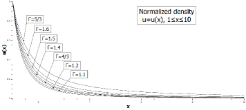
Figure 1: Dimensionless number density $u(x)=n/n_{*}$ in region $1\leq x\leq R/r_{*}=10$, $\Gamma$ from 1.1 to 5/3

As for the boundary conditions for the system of Eqns. (17), they are taken analogous to the case of Bondi-Hoyle accretion (Beskin & Pidoprygora, 1998):

$$\varepsilon^{2}g_{m}(1)=\frac{(2m)!}{2^{m}(m+1)m!}\left[\frac{(\delta E_{\rm n})_{m}}{c_{*}^{2}}-\frac{(L_{n}^{2}/\sin^{2}\theta)_{m}}{2c_{*}^{2}r_{*}^{2}}\right],$$ (24)

$$g^{\prime}_{m}(R/r_{*})=0,$$ (25)

where $(...)_{m}$ stands for the expansion in terms of the Legendre polynomials, which can be found from energy and angular momentum integral perturbations.

3 Solitary curl

Now let us consider in detail the internal structure of the quasi-spherical accretion with a small axisymetric perturbation localised near the axis $\theta=\pi$. In other words, we suppose that the angular size of the vortex is small enough ($\delta\theta_{\rm curl}\ll 1$). The main goal of this numerical calculation is to find the disturbance function $f(r,\theta)$ which gives us the possibility to determine velocity components $v_{\theta}$ and $v_{\varphi}$, i.e., the main characteristics of the perturbed flow.

To model the internal structure of the vortex, we determine $\theta$-dependent angular velocity $\Omega(\theta)$ in the form

$$\Omega(\theta)=\Omega_{0}\exp[-\alpha^{2}(1+\mathrm{cos}~{}\theta)].$$ (26)

Here $\Omega_{0}$ gives the amplitude of considered curl and the coefficient $\alpha\simeq 10$ (which are free parameters of our model) is an inversed curl width. Certainly, we assume that the perturbation is small in comparison with the main contribution of the radial accretion.

Then the flow structure can be described by the system (17), (21)–(25) formulated in previous section. As to the expansion coefficients $k_{m}$, $\lambda_{m}$ and $\sigma_{m}$, they are to be determined from Eqns. (18)–(20) and (24) on the outer boundary of a flow $r=R$. For our choice (26) the disturbances have the form

$$\delta E_{\rm n}(\theta)=\frac{{\Omega_{0}^{2}\exp[-2\alpha^{2}(1+\mathrm{cos}~{}\theta)]R^{2}\sin^{2}\theta}}{2}+{o(\varepsilon^{3})},$$ (27)

$$\delta L_{\rm n}(\theta)={\Omega_{0}\exp[-\alpha^{2}(1+\mathrm{cos}~{}\theta)]R^{2}\sin^{2}\theta}.$$ (28)

As one can easily check, it gives $\varepsilon=\Omega_{0}R/c_{\ast}$.

Expansions (18), (19), and (20) in terms of $Q_{m}(\theta)$ contain some numerical difficulties because the set of this functions is not an orthogonal one, and, even though it converges, in our case of very small curl width we can neglect just summands with numbers larger than 50. Even in some trivial cases like $\Omega(\theta)\sim(1-\theta^{2})$ these polynomials call a number of numerical obstacles (e.g., bad-conditioned matrix of linear equation for coefficients $k_{m}$, $\lambda_{m}$ and $\sigma_{m}$, etc).

In order to expand functions of integrals, we used the auxiliary set of Chebyshev polynomials, which is orthogonal and posesses a feature of generally faster convergence. Using these polynomials, we could find all expansions with the accuracy no worse than $10^{-3}$. As was shown in Sect. 2, the normalized density function $u(x)$ can be derived from the equation (21) and boundary conditions (22) and (23). The results of numerical calculations for different polytropic indeces $\Gamma$ is shown on Figure 1. In particiular, as one can see, the density is nearly constant in subsonic regime ($r\gg r_{\ast}$).

An example of the numerical calculation of perturbation function $f(r,\theta)$ is shown on Figure 2. We should stress that $f(r,\theta)$ turns actually zero outside the small region near the axial curl. This statement allows us to assume as a zero approximation that the turbulent accretion regime containing a number of curls can be considered as a set of noninteracting ones. Moving towards the accreting star, we can register that perturbation has a maximum on a radius $\sim 7r_{\ast}$, then diminishes on the distance about $2r_{\ast}$ and finally rapidly rises in the vicinity of the sonic surface $r_{\ast}$.

Apart from numerical solution, we can also find the analytical asymptotic solutions in the supersonic region $x\ll 1$ where Eqn. (17) can be rewritten as

$$g^{\prime\prime}_{m}+\frac{3}{2x}g^{\prime}_{m}+\frac{m(m+1)}{2^{\Gamma+1}}x^{-(3\Gamma+1)/2}g_{m}+\lambda_{m}\frac{R^{2}}{r_{*}^{2}}\frac{1}{4x^{3}}=O(x^{-3}).$$ (29)

Here we take into account that $\Gamma<5/3$. Getting rid of all parameters from the right part of this equation, one can introduce a new function $y_{m}=g_{m}/(\lambda_{m}R^{2}/r_{*}^{2})$. Then Eqn. (29) can be rewritten as

$$y^{\prime\prime}_{m}+\frac{3}{2x}y^{\prime}_{m}+\frac{m(m+1)}{2^{\Gamma+1}}x^{-(3\Gamma+1)/2}y_{m}+\frac{1}{4x^{3}}=O(x^{-3}).$$ (30)

Neglecting now all terms which are proportional to $x^{-\nu}$, where $\nu>-3$, we obtain that this equation has an universal solution independent of the boundary conditions on the outer boundary $r=R$

$$y(x)=-\frac{8}{x}.$$ (31)

Remember that the same asymptotic behavior was obtained by Beskin & Malyshkin (1996) for homogeneously rotating flow.

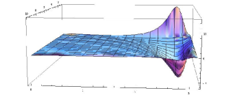
Figure 2: Disturbance function $f(r,\theta)$ in region $1\leq x\leq R/r_{*}=10$, $0\leq\theta\leq\pi$, $\Gamma=4/3$

As was already stressed, numerical results allow us to determine $v_{\theta}/v_{\varphi}$ ratio around the curl. It is easy to show that

$$\frac{v_{\theta}}{v_{\varphi}}=2\sqrt{2}\,\varepsilon\pi\left(\frac{r_{*}}{R}\right)^{7/2}p(r,\theta),$$ (32)

where

$$p(r,\theta)=\frac{\displaystyle\sum_{m=0}^{\infty}g^{\prime}_{m}(r)Q_{m}(\theta)}{\displaystyle u(r)\sin^{2}\theta\exp[-\alpha^{2}(1+\mathrm{cos}~{}\theta)]}.$$ (33)

In our calculation we put $r_{*}/R=0.1$, so that the function (33) is limited in area near the curl ($|p(r,\theta)|<200$). Taking now into account that $\varepsilon$ is a small parameter of our expansion and $|f(r,\theta)|<20$, one can show that for reasonable parameter $\varepsilon$ the ratio $|v_{\theta}/v_{\varphi}|$ in the area of vortex has an order of $\sim 10^{-5}$ (see Figure 3). Thus, we could claim that $v_{\theta}\ll v_{\varphi}$, and then one can neglect the all terms in Navier-Stokes equations that consist $v_{\theta}$.

Figure 3: $v_{\theta}/v_{\varphi}$ ratio in region $1\leq x\leq 10,19\pi/20\leq\theta\leq\pi$.

On the other hand, it is necessary to stress that, according to (31), we cannot use our solution close enough to the origin ($r\rightarrow 0$). Indeed, analysing the field line equation $\displaystyle r\rm{d}\theta/\rm{d}r=\displaystyle v_{\theta}/v_{r}$, we obtain that the asymptotic solution survives until $\theta_{0}\approx\delta\theta$, where $\theta_{0}\ll 1$ is an initial angular size of a curl and $\delta\theta$ is a broadening parameter of the stream line. Deriving $\theta$-component of the velocity from (1) and taking $v_{r}$ of zero order, we get

$$\frac{\rm{d}\theta}{{\rm d}r}\sim\varepsilon^{2}\,\displaystyle\frac{\partial f/\partial r}{\sin\theta}.$$ (34)

Assuming now that $\theta\ll 1$, one can expand equation (34) in $\theta$ and neglecting all summands of $m$ with $m\geq 2$, we find

$$\frac{\rm{d}\theta}{{\rm d}r}\sim\displaystyle\varepsilon^{2}\theta\frac{\partial}{\partial r}\frac{R^{2}}{rr_{\ast}}.$$ (35)

This equation can be simply integrated, and we obtain

$$\mathrm{ln}\frac{\theta_{0}+\delta\theta}{\theta_{0}}\sim\varepsilon^{2}\frac{R^{2}}{r_{\ast}r}.$$ (36)

Hence, under the radius $r\sim\varepsilon^{2}R^{2}/r_{\ast}$ we cannot use the solution (31) as the disturbance becomes larger than unity. In order to keep the solution up to star surface $r=r_{\rm star}$, we should demand

$$\varepsilon^{2}R^{2}/r_{\ast}<r_{\rm star},$$ (37)

where $r_{\rm star}$ corresponds to the star radius. It gives us the general condition of appliability of the approach described above. Unless we cannot use the method of linear expansion of Grad-Shafranov equation, and the turbulent flow is to be described in another way which lies outside the consideration of current paper.

Let us try now, as have been done in some papers (see, e.g., Shakura et al (2012), Shakura et al (2013)), to describe the vortex disturbance through some effective pressure, i.e., to calculate a small correction for the pressure function $P$ caused by the presence of turbulent curl. Starting with $\theta$-component of Euler equation

$$v_{r}\frac{\partial v_{\theta}}{\partial r}+v_{\theta}\frac{1}{r}\frac{\partial v_{\theta}}{\partial\theta}+\frac{v_{r}v_{\theta}}{r}-\frac{v_{\varphi}^{2}}{r}\cot\theta=-\frac{1}{r}\frac{\partial P/\partial\theta}{\rho}$$ (38)

and neglecting all the terms containing $v_{\theta}$, we obtain

$$-\frac{v_{\varphi}^{2}}{r}\cot\theta=-\frac{1}{r}\frac{\partial P/\partial\theta}{\rho}.$$ (39)

Expanding this equation near the axis and assuming

$$v_{\varphi}=\frac{L}{r\sin\theta}=\frac{K\theta}{r},$$ (40)

where $K=$ const, we obtain

$$\rho\frac{K^{2}\theta}{r^{2}}=\frac{\partial P}{\partial\theta}.$$ (41)

It gives for the additional pressure $P_{\rm add}$

$$P_{\rm add}\sim\frac{\rho K^{2}}{\alpha^{2}r^{2}},$$ (42)

where $\alpha^{-1}$ is an approximate size of a curl.

Thus, one can conclude that the pressure $P_{\rm add}$ has explicit dependence on $r$, which cannot be taken into consideration using any equation of state. Hence, we should include the turbulence into the consideration in another way than introducing effective turbulent pressure as often suggested by Shakura et al (2012, 2013).

4 Two toy models

Let us suppose now that the turbulence in the accreting matter can be described by the large number of axisymmetric vortexes with different parameters $\Omega_{0}$ and $\alpha$ filling all the accreting volume. Within this approach one can construct two toy analytical models demonstrating how the turbulence can affect the structure of the spherically symmetric accretion.

4.1 Inviscous flow

The first model in which we neglect viscosity corresponds to classical ideal spherically symmetric Bondi accretion (Bondi, 1952). In this case one can consider the following system of equations:

$$\nabla(n{\bf v}) = 0,$$ (43)

$$({\bf v}\cdot\nabla){\bf v} = -\frac{\nabla P}{\rho}-\nabla\varphi_{\rm g},$$ (44)

$$({\bf v}\cdot\nabla)s = 0.$$ (45)

Following Bondi (1952) we consider polytropic equation of state $P=P(n,s)=k(s)n^{\Gamma}$ resulting in for polytropic index $\Gamma\neq 1$

$$c_{\rm s}^{2} = \frac{\Gamma k}{m_{p}}n^{\Gamma-1},$$ (46)

$$w = \frac{c_{\rm s}^{2}}{\Gamma-1},$$ (47)

$$T = \frac{m_{p}}{\Gamma}c_{\rm s}^{2}.$$ (48)

Here again $n$ ($1/{\rm cm}^{3}$) is the number density, $m_{\rm p}$ (in ${\rm g}$) is the mass of particles ($\varrho=m_{\rm p}n$ is the mass density), $s$ is the entropy per one particle (dimensionless), ${w}$ (in ${\rm cm}^{2}/{\rm s}^{2}$) is the specific enthalpy, $T$ (in ${\rm erg}$) is the temperature in energy units, and, finally, $c_{\rm s}$ (${\rm cm/s}$) is the sound velocity.

As was demonstrated above, for a weak enough turbulence level (37) for any inividual curl one can neglect $\theta$-component of the velocity perturbation in comparison with the toroidal one $v_{\varphi}$ up to the central body $r=r_{\rm star}$. Thus, in zero approximation one can put $v_{\theta}=0$, i.e., $\theta=$ const. This implies that, according to the angular momentum concervation law $r\sin\theta~{}v_{\varphi}=$ const, we can write down

$$v_{\varphi}(r,\theta)=\Omega(\theta)\frac{R^{2}}{r}\sin\theta.$$ (49)

Here $\Omega(\theta)$ is a smooth function of $\theta$ that can be approximately described as:

$$\Omega(\theta)\approx\begin{cases}\Omega_{0},&\pi-\alpha^{-1}<\theta<\pi,\\ 0&0<\theta<\pi-\alpha^{-1}.\end{cases}$$ (50)

In order to find the characteristic values of the accretion flow we have to use energy and momentum intergals conserving on stream lines. Taking into account an assertion $v_{r}\gg v_{\varphi}\gg v_{\theta}$, we can neglect $\theta$-component of velocity which gives

$$E_{\rm n}(\theta) = \frac{v_{r}^{2}(r)}{2}+\omega(r)+\varphi_{\rm g}(r)+\frac{L^{2}(\theta)}{2r^{2}\sin^{2}\theta},$$ (51)

$$L_{\rm n}(\theta) = v_{\varphi}r\sin\theta=\Omega(\theta)r^{2}\sin^{2}\theta.$$ (52)

Averaging now these integrals in $\theta$ and introducing a new value

$$L_{\rm av}^{2}\equiv\langle\frac{L^{2}(\theta)}{\sin^{2}\theta}\rangle$$ (53)

we obtain for the averaged energy integral

$$E_{\rm av}\equiv\langle E_{\rm n}(\theta)\rangle=\frac{v_{r}^{2}(r)}{2}+\omega(r)+\underbrace{\varphi_{\rm g}(r)+\frac{L_{\rm av}^{2}}{2r^{2}}}_{\varphi_{\rm eff}(r)}.$$ (54)

As we see, two last terms can be considered as effective gravitational potential.

Futher calculations are quite similar to the classical Bondi problem for the spherical flow. In other words, using another integrals of motion, i.e., the total particle flux

$$\Phi=4\pi r^{2}n(r)v_{r}(r)=\mathrm{const},$$ (55)

and the entropy $s$, one can rewrite the energy integral (54) as

$$E_{\rm av}=\frac{\Phi^{2}}{32\pi^{2}n^{2}r^{4}}+\frac{\Gamma k(s)}{\Gamma-1}\frac{n^{\Gamma-1}}{m_{p}}-\frac{GM}{r}+\frac{L_{\rm av}^{2}}{2r^{2}}.$$ (56)

It gives the following expression for the logarithmic $r$-derivative of the number density

$$\eta_{1}=\frac{r}{n}\frac{{\rm d}n}{{\rm d}r}=\frac{\displaystyle 2-\frac{GM}{v_{r}^{2}r}+\frac{L_{\rm av}^{2}}{v_{r}^{2}r^{2}}}{\displaystyle-1+\frac{c_{\rm s}^{2}}{v_{r}^{2}}}.$$ (57)

As for Bondi accretion, this derivative has a singularity on the sonic surface ${v_{r}}=c_{\rm s}=c_{\ast}$. This implies that for smooth transition through the sonic surface $r=r_{\ast}$, the additional condition is to be satisfied:

$$2-\frac{GM}{c_{\ast}^{2}r_{\ast}}+\frac{L_{\rm av}^{2}}{c_{\ast}^{2}r_{\ast}^{2}}=0.$$ (58)

Solving now (58) in terms of $r_{\ast}$ in this approximation, we find

$$r_{*} = \frac{GM}{2c_{*}^{2}}\left(1-\frac{4L_{\rm av}^{2}c_{*}^{2}}{G^{2}M^{2}}\right),$$ (59)

$$c_{*} = \sqrt{\frac{2}{5-3\Gamma}}c_{\infty}\left(1+\frac{12(\Gamma-1)}{(5-3\Gamma)^{2}}\,\frac{L_{\rm av}^{2}c_{\infty}^{2}}{G^{2}M^{2}}\right),$$ (60)

where $c_{\infty}$ is evaluated from

$$E_{\rm av}=\frac{c_{\infty}^{2}}{\Gamma-1}.$$ (61)

Accordingly, we obtain for $r_{\ast}/r_{\ast\rm{B}}$ and $c_{\ast}/c_{\ast\rm{B}}$ ratios:

$$\frac{r_{\ast}}{r_{\ast\rm{B}}} = 1-\frac{16}{(5-3\Gamma)^{2}}\,\frac{L_{\rm av}^{2}c_{\infty}^{2}}{G^{2}M^{2}},$$ (62)

$$\frac{c_{\ast}}{c_{\ast\rm{B}}} = 1+\frac{12(\Gamma-1)}{(5-3\Gamma)^{2}}\,\frac{L_{\rm av}^{2}c_{\infty}^{2}}{G^{2}M^{2}},$$ (63)

where $c_{\ast\rm{B}}$ and $r_{\ast\rm{B}}$ correspond to the classical Bondi accretion. Finally, using the definition (53) for $L^{2}_{\rm av}$, we can rewrite our criteria of the appliability (37) as $L^{2}_{\rm av}\ll GMr_{\rm star}$. As $r_{\rm star}<r_{\ast}$, it can be finally rewritten as

$$L_{\rm av}\ll\frac{GM}{c_{\ast}}.$$ (64)

To sum up, one can conclude that the nonzero angular momentum effectively decreases the gravitational force. In other words, the presence of the angular momentum do not allow matter to fall down as easy as in its absence. Roughly speaking, we substitute our gravitating center with one that posesses less mass. So, in the case of Bondi accretion with a small angular momentum perturbation we should modify the relations for sonic surface radius and velocity — they decrease and rise respectively. It is important to note that we can consider turbulent accretion regime as one with a modified gravity potential.

4.2 Viscous flow

Figure 4: Ratio $\Omega/\Omega_{0}=F(\theta)$ for $0\leq\theta\leq\pi/30$

It this subsection we consider stationary axisymmetric quasi-spherical flow of viscous fluid. Using the condition $v_{r}\gg v_{\varphi}\gg v_{\theta}$, and neglecting all the terms containing $v_{\theta}$, we obtain for $\varphi$-component of Euler equation (Landau & Lifshits, 1987)

$$v_{r}\frac{\partial v_{\varphi}}{\partial r}+\frac{v_{r}v_{\varphi}}{r}=\nu\left(\nabla^{2}v_{\varphi}-\frac{v_{\varphi}}{r^{2}\sin^{2}\theta}\right).$$ (65)

For viscous flow it is convenient to determine the toroidal component of the velocity $v_{\varphi}$ as

$$v_{\varphi}=\Omega(r,\theta)r\sin\theta,$$ (66)

where we will use the following form for the angular velocity $\Omega(r,\theta)$:

$$\Omega(r,\theta)=\Omega_{0}(r)\exp\left[-\frac{\theta^{2}}{2\delta(r)}\right].$$ (67)

Here $\Omega_{0}=\Omega_{0}(r)$ is an amplitude, and $\delta=\delta(r)$ is a square of effective angular width of an individual curl. Substituting now $v_{\varphi}$ into Eqn. (65), we obtain

$$\dot{M}\frac{\rm d}{{\rm d}r}(\Omega r^{2}\sin\theta)=\frac{4\pi r^{2}\eta}{\sin^{2}\theta}\frac{\rm d}{{\rm d}\theta}\left[\sin^{3}\theta\frac{{\rm d}\Omega}{{\rm d}\theta}\right],$$ (68)

where

$$\dot{M}=4\pi r^{2}\rho v_{r}$$ (69)

is the accretion rate remaining constant in stationary flow, and $\eta=\rho\nu$ is a dynamic viscous coefficient which can be considered as a constant as well (Landau & Lifshits, 1987).

Using now Eqn. (68), one can easily show that the total angular momentum of an individual vortex conserves (${\rm d}L/{\rm d}r=0$). Indeed, internal friction connecting with viscosity cannot change the total angular momentum of the accreting matter. For this reason, together with (69), the angular momentum

$${\rm d}L=\rho\Omega r^{2}\sin^{2}\theta{\rm d}\phi\sin\theta{\rm d}\theta r^{2}{\rm d}r$$ (70)

can be rewritten as a full $\theta$-derivative. This implies that the r.h.s. of Eqn. (70) intergated over $\theta$ becomes zero.

Further, to determine the radial dependence of the curl amplitude $\Omega_{0}(r)$ and the squared width $\delta(r)$, we substitute the angular velocity $\Omega_{0}(r,\theta)$ (67) into (65) and expand it in terms of $\theta$ near the axis, neglecting all the terms with the power more than 3. As a result, we obtain two equations for $\Omega_{0}(r)$ and $\delta(r)$

$$\frac{\dot{M}}{2\pi\eta}r\Omega_{0}(r)+\frac{4r^{2}\Omega_{0}(r)}{\delta(r)}+\frac{\dot{M}}{4\pi\eta}r^{2}\Omega_{0}^{\prime}(r)=0,$$ (71)

$$\begin{split}-18r^{2}\Omega_{0}(r)-\frac{3\dot{M}}{2\pi\eta}r\delta(r)\Omega_{0}(r)-10r^{2}\delta(r)\Omega_{0}(r)-\\ \frac{\dot{M}}{2\pi\eta}r\delta^{2}(r)\Omega_{0}(r)+\frac{3\dot{M}}{4\pi\eta}r^{2}\delta^{\prime}(r)\Omega_{0}(r)-\frac{\dot{M}}{4\pi\eta}r^{2}\delta^{2}(r)\Omega_{0}^{\prime}(r)=0,\end{split}$$ (72)

which have simple solutions

$$\delta(r) = \delta_{0}+\frac{8\pi\eta(r-r_{0})}{\dot{M}},$$ (73)

$$\Omega_{0}(r) = \Omega_{0}\frac{r_{0}^{2}}{r^{2}}\left[\frac{8\pi\eta(r-r_{0})}{\dot{M}\delta_{0}}+1\right]^{-2}.$$ (74)

Introduction of a small vortex tubulence can be again treated by modifying a gravitational potential as

$$\varphi_{\rm{eff}}=\displaystyle-\frac{GM}{r}+\frac{\Omega_{0}^{2}r_{0}^{4}\delta_{0}}{4\pi r^{2}}\left[\displaystyle 1+\frac{8\pi\eta}{\dot{M}\delta_{0}}(r-r_{0})\right]^{-3}.$$ (75)

Thus, viscosity results in increasing of the vortex width ($\delta^{\prime}<0$ for ${\dot{M}<0}$ corresponding to accretion) and diminishing of the angular rotation. On the other hand, the role of viscosity will be small if

$$\frac{8\pi\eta r_{0}}{|\dot{M}|\delta_{0}}\ll 1.$$ (76)

For $\eta\rightarrow 0$ we return to the previous result $\delta(r)=$ const, $\Omega_{0}(r)\propto r^{-2}$. Introducing now Reynolds number as

$${\rm Re}=\frac{\rho vl}{\eta},$$ (77)

where $\rho,v$ and $l=r_{0}\delta^{1/2}$ are characteristic values of a flow and using expression (69), we can rewrite (76) as

$${\rm Re}=\frac{|\dot{M}|}{4\pi r_{0}\eta}\gg\delta_{0}^{-1/2}.$$ (78)

This implies that the role of viscosity is small for turbulent flow.

Certainly, the analysis presented above allows us to take into consideration only isolated set of curls. In reality, dense celluar turbulent structure posesses a number of collective effects (Prokhorov, Popov & Khoperskov, 2002), that is to be described in another way. The easiest method to proceed with the minimal number of additional assumptions is to choose another angular velocity profile.

As the total angular momentum of the accreting matter is suppose to be zero, we will use the following expression for the angular velocity

$$\Omega(r,\theta)=\Omega_{0}(r)\exp\left(-\frac{\theta^{2}}{2\delta}\right)\left(1-\frac{\gamma^{2}}{2\delta}\theta^{2}\right).$$ (79)

Here the parameter $\gamma$ is to be chosen from the condition of the zero total angular momentum

$$\int_{|\vec{r}|\leq R}{\rm d}L=0,$$ (80)

which is equivalent to

$$\int_{0}^{\pi}d\theta\sin^{3}\theta\,\Omega(r,\theta)=0.$$ (81)

One of its realisations can be seen on Figure 4 where the dashed line shows zero angular velocity level. Configuration like this one represents the unit of celluar turbulent structure, fulfilling main requirements of its nature. To simplify our calculations, we hold $\gamma$ and $\delta$ on constant values in order to get simple equation on $\Omega_{0}(r)$. Again, we expand equation (68) in terms of $\theta$ to the first order. As a result, we obtain for $\Omega_{0}(r)$:

$$\Omega_{0}(r)=\Omega_{0}\left(\frac{r_{0}}{r}\right)^{2}\exp\left[\frac{16\pi\eta}{\dot{M}}\frac{(1+\gamma^{2})}{\delta}(r_{0}-r)\right].$$ (82)

In this case, the effective gravitational potential cannot be derived for arbitary parameters without special functions. It can be written as

$$\varphi_{\rm{eff}}=\displaystyle-\frac{GM}{r}+C\cdot\frac{\displaystyle\Omega_{0}^{2}r_{0}^{4}}{\displaystyle r^{2}}\exp\left[-\frac{16\pi\eta}{|\dot{M}|}\frac{(1+\gamma^{2})}{\delta}(r_{0}-r)\right],$$ (83)

where

$$C=\frac{1}{2\pi}\int_{0}^{\pi}\rm{d}\theta\exp(-\theta^{2}/\delta)(1-\frac{\gamma^{2}\theta^{2}}{2\delta})^{2}\sin^{2}\theta.$$ (84)

Choosing, for instanse, $\gamma=1/\sqrt{2}$ and $\delta=10^{-4}$, it gives $C\approx 3.4\cdot 10^{-8}$.

The expression under the exponential function in (82) is always lower than zero, so the criterion of the importance of viscosity effects can be formulated as

$$\frac{16\pi\eta}{|\dot{M}|}\frac{(1+\gamma^{2})}{\delta}r_{0}\gg 1,$$ (85)

which is more convinient to discuss in terms of Reynolds number

$$\delta^{-1/2}\gg{\rm Re}.$$ (86)

Thus, for narrow vortex (i.e., for $\delta<10^{-2}$) the viscosity effects must be taken into account.

5 Conclusion

We have shown that in the case of the vortex turbulence represented by a solitary axisymmetric curl, one cannot simulate effects of the turbulence by introduction of the effective pressure which is common in recent papers (see, e.g., Shakura et al (2012), Shakura et al (2013)). On the other hand, it is possible to take into account the vortex structure of the accreting flow by introducing an effective gravitational potential.

Further, we described two analytical toy models that show how the turbulence affects the structure of the spherically symmetric flow. In particular, it was shown that the sonic surface moves inwards because of effective diminishing of gravitational force. Finally, a criterion to analyze the importance of viscosity effects in the adiabatic flow filled either by isolated or dense set of curls was formulated.

We thank K.P. Zybin for useful discussions. This work was partially supported by Russian Foundation for Basic Research (Grant no. 14-02-00831)

References

• Anderson (1989) Anderson M., 1989, MNRAS, 239, 19
• Axford & Newman (1967) Axford W. I. & Newman R. C., 1967, Astrophys. J., 147, 230
• Balbus & Hawley (1989) Balbus S. A. & Hawley J. F., 1991, Astrophys. J., 376, 214
• Beskin (2010) Beskin V.S., MHD Flows in Compact Astrophysical Objects, 2010. Springer, Berlin
• Beskin & Malyshkin (1996) Beskin V. S. & Malyshkin L. M., 1996, Astron. Lett., 22, 475
• Beskin & Pidoprygora (1995) Beskin V. S. & Pidoprygora Yu. N., 1995, JETP 80, 575
• Beskin & Pidoprygora (1998) Beskin V. S. & Pidoprygora Yu. N., Astron. Rep., 1998, 42, 71
• Bhattacherjee & Ray (2005) Bhattacherjee J. K. & Ray A. K., 2005, Astrophys. J., 627, 368
• Bisnovatyi-Kogan et al (1979) Bisnovatyi-Kogan G.S., Kazhdan Ya.M., Klypin A. A. et al., 1979, Sov. Astron. 23, 201
• Bondi (1952) Bondi H., 1952, MNRAS, 112, 195
• Bondi & Hoyle (1944) Bondi H. & Hoyle F., 1944, MNRAS, 104, 272
• Brandenburg & Sokoloff (2002) Brandenburg A. & Sokoloff D. D., 2002, Geophys. Astrophys. Fluid Dyn., 96, 319
• Heyvaerts (1996) Heyvaerts J., 1996, in Chiuderi C., Einaudi G. eds, Plasma Astrophysics. Springer, Berlin, p. 31
• Hunt (1979) Hunt R.,, 1979, MNRAS, 198, 83
• Kovalenko & Eremin (1998) Kovalenko I. G. & Eremin M. A., 1998, MNRAS, 298, 861
• Krolik & Hawley (1979) Krolik J. & Hawley J. F., 1991, Astrophys. J., 573, 754
• Landau & Lifshits (1987) Landau L. D. & Lifshits E. M. Fluid Mechanics, 1987. Pergamon Press, Oxford
• Lipunov (1992) Lipunov V. M., Astrophysics of Neutron Stars, 1992, Springer, Heidelberg
• Pariev (1996) Pariev V. I., 1996, MNRAS, 283, 1264
• Petrich et al (1988) Petrich L. I., Shapiro S., & Teukolsky S., 1988, Phys. Rev. Lett, 60, 1781
• Petrich et al (1989) Petrich L.I., Shapiro S., Stark R. F., & Teukolsky S., 1989, Astrophys. J., 336, 313
• Prokhorov, Popov & Khoperskov (2002) Prokhorov M. E., Popov S. B., Khoperskov A.V. 2002, Astron. Astrophys., 381, 1000
• Ruffert & Arnett (1994) Ruffert M. & Arnett D., 1994, Astron. Astrophys., 346, 861
• Shakura et al (2013) Shakura N. I., Postnov K. A., Kochetkova A. Yu.& Yalmasdotter L., 2013, Phys. Usp., 183, 337
• Shakura et al (2012) Shakura N. I., Postnov K. A., Kochetkova A. Yu.& Yalmasdotter L., 2012, MNRAS, 420, 216
• Shapiro & Teukolsky (1983) Shapiro S. & Teukolsky S., Black Holes, White Dwarfs, and Neutron Stars: The Physics of Compact Objects, 1983, Wiley, New York
• Shcherbakov (2008) Shcherbakov R. V., 2008, Astrophys. J. S., 177, 493S
• Toropin et al. (1999) Toropin Yu. M., Toropina O. D., Saveliev V. V., et al., 1999, Astorphys. J., 593, 472
• Toropina et al. (2012) Toropina O. D., Romanova M. M. & Lovelace R. V. D., 2012, MNRAS, 420, 810