On the Hilbert Geometry of Convex Polytopes

Abstract

We survey the Hilbert geometry of convex polytopes. In particular we present two important characterisations of these geometries, the first one in terms of the volume growth of their metric balls, the second one as a bi-lipschitz class of the simplexe’s geometry.

1 Introduction

Our understanding of the Hilbert geometry associated to the interior of a convex polytope has increased tremendeously in the last decade. Polytopes play an important role in the realm of Hilbert geometries because they are related to linear programming and their geometry is somehow more amenable and simple than that of general convex sets.

This chapter aims at presenting various results and characterisations of the Hilbert geometry of polytopes. For instance their group of isometries is now well understood (see Section 4). Their volume growth is polynomial and its order characterises them (Section 5). They are the only Hilbert geometry which can be isometrically embedded in a normed vector space (see Section 6). For a given dimension, they all belong to the same bi-Lipschitz class with the Euclidean metric space (see Section 7).

When it was enlightening we dared offer our own proofs on some of the results presented here. Hence one will find an outline of a new proof that in dimension $2$ the unique Hilbert geometry isometric to a normed vector space is the one associated to a triangle. We also show that any polytope with $N+1$ faces can be isometrically embedded in a normed vector space of dimension $N$. This last results improves the dimension of the target space which was previously known to be $N(N+1)/2)$ [21], and is more geometric in nature than the previous proofs. We end this chapter by outlining a proof of the fact that the Hilbert geometry of a polytope is bi-Lipschitz equivalent to a normed vector space of the same dimension.

2 Definitions related to Hilbert Geometry, polytopes and notation

2.1 Hilbert Geometries

Let us recall that a Hilbert geometry $(\mathcal{C},d_{\mathcal{C}})$ is a non-empty bounded open convex set $\mathcal{C}$ on ${\mathbb{R}}^{n}$, that we shall call convex domain, with the Hilbert distance $d_{\mathcal{C}}$ defined as follows : for any distinct points $p$ and $q$ in $\mathcal{C}$, the line passing through $p$ and $q$ meets the boundary $\partial\mathcal{C}$ of $\mathcal{C}$ at two points $a$ and $b$, such that someone walking on the line goes consecutively by $a$, $p$, $q$, $b$ (Figure 1). Then we define

$$d_{\mathcal{C}}(p,q)=\frac{1}{2}\log[a,p,q,b],$$

where $[a,p,q,b]$ is the cross-ratio of $(a,p,q,b)$, i.e.,

$$[a,p,q,b]=\frac{\|q-a\|}{\|p-a\|}\frac{\|p-b\|}{\|q-b\|}>1,$$

and $\|\cdot\|$ is the standard Euclidean norm in $\mathbb{R}^{n}$.

Figure 1: The Hilbert distance

Note that the invariance of cross-ratios under projective maps implies the invariance of $d_{\mathcal{C}}$ by such maps.

These geometries are naturally endowed with a continuous Finsler metric $F_{\mathcal{C}}$ defined as follows: if $p\in\mathcal{C}$ and $v\in T_{p}\mathcal{C}={\mathbb{R}}^{n}$ with $v\neq 0$, the straight line passing by $p$ and directed by $v$ meets $\partial\mathcal{C}$ at two points $p^{+}$ and $p^{-}$ ; we then define

$$F_{\mathcal{C}}(p,v)=\frac{1}{2}\|v\|\biggl{(}\frac{1}{\|p-p^{-}\|}+\frac{1}{\|p-p^{+}\|}\biggr{)}\quad\textrm{and}\quad F_{\mathcal{C}}(p,0)=0.$$ (2.1)

Figure 2: The Finsler structure

The Hilbert distance $d_{\mathcal{C}}$ is the length distance associated to the Finsler metric $F_{\mathcal{C}}$.

2.2 Faces

To an arbitrary closed convex set $K$ of a real vector space we can associate an equivalence relation, stating that two points $A$ and $B$ are equivalent if there exists a segment $[C,D]\subset K$ containing the segment $[A,B]$ such that $C\neq A,B$ and $D\neq A,B$. The equivalence classes are called faces. A face is called a $k$-face when the dimension of the affine space it generates is $k$. Observe that a face is always open in the affine space it generates. As usual we call vertex a $0$-dimensional face.

In this chapter a simplex in ${\mathbb{R}}^{n}$ is the convex closure of $n+1$ affinely independent points, that is a triangle in ${\mathbb{R}}^{2}$, a tetrahedron in ${\mathbb{R}}^{3}$, etc. More generally, in this survey, a polytope in ${\mathbb{R}}^{n}$ will be the convex hull of a finite number of points, such that $n+1$ of them are affinely independent. The $n$-face of a polytope is its interior, in particular it is never empty.

The next definition is due to Benzecri [6] and plays an important role in the study of convex sets.

Definition 2.1 (Conical faces).

Let $\mathcal{C}$ be a convex set in ${\mathbb{R}}^{n}$. Let $k<n$. Suppose that a simplex $S$ contains $\mathcal{C}$ and that a non-empty $k$-face $f\subset\partial\mathcal{C}$, is included in a $k$-face of $S$. Then we say that $f$ is a conical face of $\mathcal{C}$ and that $\mathcal{C}$ admits a conical face.

Figure 3: Conical faces in dimension 3

When a face $f$ is contained in the boundary of another face $F$ we write $f<F$.

Definition 2.2 (Conical flag).

Let $\mathcal{C}$ be a convex set in ${\mathbb{R}}^{n}$. If there exists a simplex $\mathcal{S}$ contained in $\mathcal{C}$, and a sequence of faces $(f_{i})_{0\leqslant i\leqslant n-1}$ such that for any $k=0,\ldots,n-1$,

1. $\emptyset<f_{0}<f_{1}<f_{2}<\ldots<f_{n-1}<\mathcal{S}$,

2. $f_{k}$ is a subset of a $k$-conical face of $\mathcal{C}$;

3. no other $k$-face of $\mathcal{S}$ is in the interior of a $k$-conical face of $\mathcal{C}$;

then we call $f_{0}<f_{1}<f_{2}<\ldots<f_{n-1}<\mathcal{C}$ a conical flag and we say that $\mathcal{C}$ admits a conical flag. Furthermore we will call $\mathcal{S}$ a conical flag neighborhood of $\mathcal{C}$.

3 Alternate viewpoints on the Hilbert metric of Polytopes

We present here two explicit formulas arising from two different viewpoints on the Hilbert metric. The first one is due to Garett Birkhoff and the second one to Ralph Alexander. Both are useful in some applications (see Section 6).

Proposition 3.1 (G. Birkhoff [9]).

Consider a convex polytope ${\mathcal{P}}$ in $R^{n}$ defined by the $N$ affine maps $L_{1},\ldots,L_{N}\colon{\mathbb{R}}^{n}\to{\mathbb{R}}$ as follows

$${\mathcal{P}}=\{x\in{\mathbb{R}}^{n}\mid L_{i}(x)>0,1\leqslant i\leqslant N\}\text{.}$$

Then for any pair of points $(x,y)$ contained in the interior of ${\mathcal{P}}$ one has

$$d_{{\mathcal{P}}}(x,y)=\frac{1}{2}\sup_{1\leqslant i,j\leqslant N}\log\biggl{(}\dfrac{L_{i}(x)}{L_{i}(y)}\dfrac{L_{j}(y)}{L_{j}(x)}\biggr{)}\text{.}$$

This formula is a consequence of the convexity and the fact that if $z_{i}$ is the intersection of the straight line $(xy)$ with the hyperplane $H_{i}=\{L_{i}=0\}$, then by Thales’s theorem we have

$$\frac{||x-z_{i}||}{||y-z_{i}||}=\dfrac{L_{i}(x)}{L_{i}(y)}\text{.}$$

In dimension two a second point of view is available: focus on the angle defined by two lines $H_{1}$ and $H_{2}$ intersecting at a point $p$. Consider now two points $x$ and $y$ lying the interior of the same sector $Q$ defined by these two lines and let $X^{*}$ and $Y^{*}$ be the straight lines $(px)$ and $(py)$ respectively. Assuming that the four lines $H_{1}$, $X^{*}$, $Y^{*}$ and $H_{2}$ appear in that order let $h_{Q}(x,y)$ be their cross-ratio, and define

$$\delta_{Q}(x,y)=\frac{1}{2}\log h_{Q}(x,y)\text{.}$$

In other words, $\delta_{Q}$ is the cone-metric associated to the cone $Q$. It is equal to $0$ if $(px)$ and $(py)$ define the same line. If $H_{i}$ is given by the equation $L_{i}=0$ for $i=1,2$ then we have

$$\delta_{Q}(x,y)=\frac{1}{2}\Biggr{|}\log\biggl{|}\dfrac{L_{1}(x)}{L_{1}(y)}\dfrac{L_{2}(y)}{L_{2}(x)}\biggr{|}\Biggr{|}\text{.}$$ (3.2)

From this last remark we can now state the following proposition, which is a kind of Crofton formula related to the Hilbert geometry of plane polytopes, i.e., polygons. This means that we relate the length of a segment to a measure on the set of lines crossing that segment, see [3].

Proposition 3.2 (R. Alexander [1]).

Let ${\mathcal{P}}$ be a polygone with vertices $p_{1},\ldots,p_{N}$, and for $i=1,\ldots,N$ let $Q_{i}$ be the interior angle defined at the vertex $p_{i}$; then the Hilbert distance in ${\mathcal{P}}$ is given by

$$d_{{\mathcal{P}}}(x,y)=\frac{1}{2}\sum_{i=1}^{n}\delta_{Q_{i}}(x,y)\text{.}$$

To obtain this formula, it suffices to sum up the $\delta_{Q_{i}}$’s corresponding to the vertices lying on one side of the straight line $(xy)$, which gives $d_{{\mathcal{P}}}(x,y)$. A somewhat similar description in higher dimensions has been given by Rolf Schneider [27].

4 The group of isometries versus collineations for a polytopal Hilbert geometry

Let $\sigma_{n+1}$ be the group of permutations on the set $\{1,\ldots,n+1\}$ and let us denote by $\Gamma_{n+1}=\sigma_{n+1}\sigma_{2}=\sigma_{n+1}{\mathbb{Z}}/2{\mathbb{Z}}$.

Let us remind the reader that a collineation is a bijection from one projective space to another, or from a projective space to itself, such that the images of collinear points are themselves collinear. A homography is an isomorphism of projective spaces, induced by an isomorphism of the vector spaces from which they are derived. Homographie are collineations but in general not all collineations are homographies. However the fundamental theorem of projective geometry asserts that in the case of real projective spaces of dimension at least two a collineation is a homography.

Theorem 4.1.

Let $({\mathcal{P}},d_{\mathcal{P}})$ be a polytopal Hilbert geometry of dimension $n$. Then the group of isometries is isomorphic to

1. ${\mathbb{R}}^{n}\rtimes\Gamma_{n+1}$ if ${\mathcal{P}}$ is a simplex;

2. the group of collineations of ${\mathcal{P}}$ otherwise.

The first part of this theorem was known, see for instance Pierre de la Harpe [18]. The second part of the theorem is due to Bas Lemmens and Cormac Walsh [22] following ideas of Cormac Walsh [32] (see also his contribution to this handbook [33]).

Their main idea is to study the Horoboundary of a Polytopal Hilbert geometry. They show that one can define a metric, the detour metric, between Busemann points which extends somehow the Hilbert metric. For this metric the Busemann boundary is divided into different parts. Two points between different parts are at an infinite distance, in particular Busemann points related to two different faces of the polytope are not in the same part. Then their strategy consists in proving the following facts: Given an isometry $f$ between two polytopal Hilbert geometries:

1. The map $f$ defines an isometry between their respective Busemann boundaries endowed with the detour metric;

2. either $f$ maps vertex parts to vertex parts and faces to faces or $f$ interchanges them;

3. if $f$ maps vertex parts to vertex parts, then $f$ extends continuously to the boundary;

4. if $f$ extends continuously to the boundary, then it is a collineation;

5. if $f$ interchanges vertex parts and faces, then the two polytopes are simplices.

Notice that although it is now known that for a general Hilbert geometry the group of isometries is a Lie group (see L. Marquis’ contribution to this handbook [23]), it is still not known when it coincides with its group of collineations.

5 Characterisation by volume growth

Theorem 5.1.

Let $(\Omega,d_{\Omega})$ be a Hilbert geometry of dimension $n$. Let $\mathrm{Vol}$ be its Hausdorff or Holmes-Thompson measure and let $B_{\Omega}(o,R)$ be the metric ball of radius $R$ centerd at $o$. Then the upper asymptotic volume, which is defined as

$$\overline{\mathrm{Asvol}}\bigl{(}\Omega\bigr{)}=\limsup_{R\to+\infty}\dfrac{\mathrm{Vol}\bigl{(}B_{\Omega}(o,R)\bigr{)}}{R^{n}}\text{,}$$

is finite if and only if $\Omega$ is a polytope.

The fact that the upper asymptotic volume of a polytopal Hilbert geometry is finite was proved by the author in [28]. The converse is also due to the author and a complete proof can be found in [30]. More precisely, in that paper we prove the following lower bound on the asymptotic volume:

Theorem 5.2.

There exists a constant $a_{n}$ such that for any Hilbert geometry $(\Omega,d_{\Omega})$ of dimension $n$ which admits $k$ extremal points one has

$$a_{n}\cdot k\leqslant\overline{\mathrm{Asvol}}\bigl{(}\Omega\bigr{)}\text{.}$$

Hence having finite asymptotic volume implies that the convex set $\Omega$ has a finite number of extremal points and therefore is a polytope.

The proof of Theorem 5.2 relies on the identity (6.5) below and on the fact that the measure of balls of radius $R$ have a uniform lower bound of the form $b_{n}R^{n}$, for some constant $b_{n}$ depending only on the dimension (see [30]). Then it suffices to include in a ball of radius $R$, $k$-disjoint balls of radius $R/4$, centered on the geodesic rays joining the center of the ball to the extremal points. This is possible precisely thanks to the the equality (6.5).

Notice that finding a similar upper bound as in Theorem 5.2 is not yet done, and would probably solve the entropy upper-bound conjecture using the methods developed by the author in [31] to prove it in dimensions $2$ and $3$.

6 Characterisation by isometric embedding

6.1 The special case of simplices

Theorem 6.1.

Let $(\Omega,d_{\Omega})$ be a Hilbert geometry. It is isometric to a normed vector space if and only if $\Omega$ is projectively equivalent to a simplex.

The “if” part was proved by Roger Nussbaum [24] and Pierre de la Harpe [18]. The “only if” is due to Thomas Foertsh and Anders Karlsson [16].

Let us illustrate the two-dimensional case with an ad hoc proof not requiring the technicality of [16]. Let $e_{1}$, $e_{2}$ and $e_{3}$ be an affine basis of an affine plane; then the convex hull of these three points is a two-dimensional simplex $\mathcal{S}_{2}$.

Now using the barycentric coordinates attached to the family $(e_{i})_{1\leqslant i\leqslant 3}$, each point $p$ in the interior of the simplex is uniquely associated to a triple of positive real numbers $\alpha_{1},\alpha_{2},\alpha_{3}$ such that $\sum_{i}\alpha_{i}=1$ and $p=\sum_{i}\alpha_{i}e_{i}$. Therefore, one can define a map from $\mathcal{S}_{2}$ to the plane $\bigl{\{}x+y+z=0\bigr{\}}$ of ${\mathbb{R}}^{3}$ by

$$\Phi_{2}(p)=\biggl{(}\log\frac{\alpha_{1}}{\alpha_{2}},\log\frac{\alpha_{2}}{\alpha_{3}},\log\frac{\alpha_{3}}{\alpha_{1}}\biggr{)}\text{.}$$ (6.3)

This map is easily seen to be a bijection whose inverse is

$$\Phi_{2}^{-1}(x,y,z)=\frac{1}{e^{x}+e^{x+y}+1}(e^{x+y},e^{y},1)\text{.}$$ (6.4)

Finally, if ${\mathbb{R}}^{3}$ is endowed with the sup norm, then this map is an isometry.

Now, the intersection of the unit cube of ${\mathbb{R}}^{3}$ with the plane $x+y+z=0$ is a regular hexagon, and therefore we deduce from this that the Hilbert geometry of a simplex is isometric to ${\mathbb{R}}^{2}$ endowed with a norm whose unit ball is a regular hexagon.

Conversely, and without loss of generality, suppose that $\Omega$ is a planar bounded convex set whose Hilbert geometry is isometric to a two-dimensional normed vector space. Since its volume growth being polynomial of order two, it follows, from [30], that $\Omega$ is necessarily a polygon. Besides, in dimension $2$, the length of a sphere of radius $R$ in a normed vector space is $cR$ for a constant $6\leqslant c\leqslant 8$. However in a polygon with $n$ vertices a simple computation shows that as $R$ goes to infinity, the length of a sphere of radius $R$ is equivalent to $2nR$. Hence, $n=3$ or $4$. The case $n=4$ would mean that $\Omega$ is a convex quadrilateral, which is projectively equivalent to a square; however the square is not isometric to a normed vector space, as in the center the finsler norm is a square, on the diagonals an hexagon and elsewhere an octagon. Therefore, $n=3$ and $\Omega$ is a triangle.

6.2 Isometric embeddings of polytopes

Theorem 6.2.

For a convex domain $\Omega\subset\mathbb{R}^{n}$, the following conditions are equivalent:

1. $\Omega$ is a bounded polytope.

2. The Hilbert geometry $(\Omega,d_{\Omega})$ can be isometrically embedded in a finite dimensional normed vector space

Observe that condition (b) means that there exists a norm $\|\cdot\|$ on $\mathbb{R}^{m}$ for some $m\in\mathbb{N}$, and a map $f:(\Omega,d_{\Omega})\to(\mathbb{R}^{m},\|\,\|)$ which is an isometry onto its image. By Theorem , the image $f(\Omega)\subset\mathbb{R}^{m}$ is an affine subspace if and only if $\Omega$ is a simplex.

The implication $(a)\Rightarrow(b)$ is due to Brian Lins who proved it in his dissertation [21]. He used Birkhoff’s result Proposition 3.1 and obtained an embedding $f:\Omega\to\mathbb{R}^{N(N+1)/2}$ for the sup norm, where $N$ is one less the number of faces of the polytope.

A more geometric proof of this implication is to see it as an immediate consequence of Theorem 6.1, together with the following result which states that any bounded polytope is affinely equivalent to the intersection of a simplex and an affine subspaces in some vector space (see also [17] Theorem 1 in section 5.1). The argument also reduces the dimension of the ambient space from $N(N+1)/2$ to $N$.

Proposition 6.3.

Let ${\mathcal{P}}$ be a convex and bounded polytope in ${\mathbb{R}}^{n}$ with $N+1$ $(n-1)$-faces. Then there exists an $N$-simplex $S_{N}$ and an $n$-dimensional affine space $A_{n}$ in ${\mathbb{R}}^{N}$ such that ${\mathcal{P}}$ is affinely equivalent to $A_{n}\cap S_{N}$.

Proof.

Let $L_{i}\colon{\mathbb{R}}^{n}\to{\mathbb{R}}$ be affine function, for $1\leqslant i\leqslant N+1$ such that

$${\mathcal{P}}=\{x\in{\mathbb{R}}^{n}\mid L_{i}(x)>0,1\leqslant i\leqslant N+1\}\text{.}$$

Notice that necessarily $N\geqslant n$ for the convex to be bounded. Let the family $(e_{i})_{1\leqslant i\leqslant n+1}$ be an affine basis of ${\mathbb{R}}^{n}$ and let us suppose that in that basis, one has, in barycentric coordinates $x=\sum_{i}x_{i}e_{i}$ and $\sum_{i}x_{i}=1$,

$$L_{i}(x)=a_{1}^{i}x_{1}+\cdots+a_{n+1}^{i}x_{n+1}\text{,}$$

where for each $1\leqslant i\leqslant n+1$ the $a_{j}^{i}$ are not all equal and, without loss of generality, we can suppose that the first $n+1$ hyperplanes are affinely independent.

Now let us consider an affine basis $(f_{i})_{1\leqslant i\leqslant N+1}$ of ${\mathbb{R}}^{N}$, and then define the following affine functions from ${\mathbb{R}}^{N}$ to ${\mathbb{R}}$, with $y=\sum_{i}y_{i}f_{i}$ and ${\sum_{i}y_{i}=1}$,

$$H_{i}(y)=\\ \begin{cases}a_{1}^{i}y_{1}+\cdots+a_{n+1}^{i}y_{n+1}&\text{for }1\leqslant i\leqslant n+1\\ a_{1}^{i}y_{1}+\cdots+a_{n+1}^{i}y_{n+1}+y_{i}&\text{for }n+2\leqslant i\leqslant N+1\end{cases}\text{.}$$

Then the affine hyperspaces $\{H_{i}=0\}$ for $1\leqslant i\leqslant N+1$ are affinely independant points in the dual space, hence

$$S_{N}=\bigl{\{}y\mid H_{i}(y)>0,1\leqslant i\leqslant N+1\bigr{\}}$$

is an $N$-simplex of ${\mathbb{R}}^{N}$. Now notice that the intersection of that simplex with the affine space

$$A_{n}=\{y\mid y_{n+2}=\cdots=y_{N+1}=0\}$$

is affinely equivalent to ${\mathcal{P}}$, using the map

$$(x_{1},\ldots,x_{n+1})\mapsto(x_{1},\ldots,x_{n+1},0,\ldots,0)\text{.}$$

∎

The implication $(b)\Rightarrow(a)$ in Theorem 6.2 is due to Bruno Colbois and Patrick Verovic [15], who actually proved that if one can quasi-isometrically embed a bounded Hilbert geometry $(\Omega,d_{\Omega})$ into a finite dimensional normed vector space $(V,||\cdot||)$, then the boundary $\partial\Omega$ admits at most a finite number of extremal points. Let us make a slight variation of their proof, assuming an isometric embedding $f\colon(\Omega,d_{\Omega})\to(V,||\cdot||)$ is given. The proof relies on the following important two facts:

1. The unit sphere of a normed vector space of finite dimension is compact, therefore a maximal set of $1$-separated points (i.e. a set in which any two distinct points are at distance at least $1$) is finite. Let $N$ be the cardinality of such a set.

2. If $x_{\infty}$ and $y_{\infty}$ are two extremal points on the boundary $\partial\Omega$ of a Hilbert geometry with supporting hyperplanes not containing the line $(x_{\infty}y_{\infty})$; $o$ a point in $\Omega$; $x(t)$, $y(t)$ two geodesics rays from $o$ to respectively $x_{\infty}$ and $y_{\infty}$; then

   $$\lim_{t\to\infty}\dfrac{d_{\Omega}\bigl{(}x(t),y(t)\bigr{)}}{2t}=1\text{.}$$ (6.5)

Now let us suppose that the boundary $\partial\Omega$ admits $N+1$ distinct extremal points $x^{1}_{\infty},\ldots,x_{\infty}^{N+1}$ with suppoting hyperplanes not containing any two of them, and let us fix a point $o$ in $\Omega$ and suppose that the image of $o$ is the origin of $V$. Let us denote by $x^{i}(t)$ a geodesic ray from $o$ to $x^{i}_{\infty}$.

Then for any positive real number $t\in{\mathbb{R}}^{+}_{*}$ we have on the one hand

$$\left\|\frac{f(x^{i}(t)}{t}\right\|=\dfrac{d_{\Omega}\Bigl{(}o,f\bigl{(}x^{i}(t)\bigr{)}\Bigr{)}}{t}=1$$ (6.6)

hence $f(x^{i}(t)/t$ lies on the unit sphere of $(V,||\cdot||)$. On the other hand, using the formula (6.5) we can find $T\in{\mathbb{R}}^{+}$ such that for any $1\leqslant i<j\leqslant N+1$ and $t>T$,

$$\left\|\frac{f(x^{i}(t)}{t}-\frac{f(x^{j}(t)}{t}\right\|=\dfrac{d_{\Omega}\bigl{(}x^{i}(t),y^{j}(t)\bigr{)}}{t}\geqslant 1\text{.}$$ (6.7)

Therefore, for $t>T$, the family $\bigl{(}f(x^{i}(t))/t\bigr{)}$ is a $1$-separated family on the unit sphere, which admits $N+1$ points. This is in contradiction with the maximality of $N$. Hence the boundary $\partial\Omega$ admits no more than $N$ such extremal points.

Now if $\Omega$ is not a polytope, it admits a two-dimensional section wich is not a polygon, and then by Krein-Millman’s Theorem we can find a sequence of distinct extremal points whose supporting lines do not contain any two of them. Hence we cannnot embed it into a normed vector space.

7 Polytopal Hilbert geometries are bi-Lipschitz to Euclidean vector spaces

Theorem 7.1.

An $n$-dimensional polytopal Hilbert geometry $({\mathcal{P}},d_{\mathcal{P}})$ is bi-Lipschitz equivalent to the $n$-dimensional Euclidean geometry (${\mathbb{R}}^{n},\|\cdot\|)$. In other words, there exists a map $\Phi\colon{\mathcal{P}}\to{\mathbb{R}}^{n}$ and a constant $A$ such that for any two points $x$ and $y$ in ${\mathcal{P}}$,

$$\frac{1}{A}\cdot\|\Phi(x)-\Phi(y)\|\leqslant d_{\mathcal{P}}(x,y)\leqslant A\cdot\|\Phi(x)-\Phi(y)\|\text{.}$$

This theorem was proved by Bruno Colbois, Patrick Verovic and Constantin Vernicos in dimension $2$ [13], and independently by Andreas Bernig [8] and by the author [29] in all dimensions.

Both proofs consist in building a bi-Lipschitz map. A. Bernig shows that if the convex polytope is defined by $N$ affine maps $L_{1},\ldots,L_{N}$ as follows

$${\mathcal{P}}=\{x\mid L_{i}(x)>0,1\leqslant i\leqslant N\}\text{,}$$

then the map

$$x\mapsto\Phi_{b}(x)=\sum_{i=1}^{N}\log L_{i}(x)\cdot dL_{i}$$

is a bi-Lispchitz map onto the dual vector space (notice that the linear part of $L_{i}$ coincides with $dL_{i}$). This map is easily seen to be Lipschitz continuous. The difficult part in A. Bernig’s proof is to show that this map is onto.

Our construction is more geometric and the map we build is easily seen to be a bijection. The tricky part is to prove that it is a bi-Lipschitz map. Our proof recedes through the following four steps:

1. Using the barycentric subdivision, we decompose a polytopal $\cal P$ domain of ${\mathbb{R}}^{n}$ into a finite number of simplices $S_{i}$, which we call barycentric simplexes and which happen to be conical flag neighborhoods of the polytope.

         

   

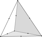
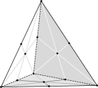
   Figure 4: The last three steps of the decomposition in dimension $3$

2. The second steps consists in proving that each simplex $S_{i}$ admits a bi-lipschitz embedding $L_{i}$ onto a fixed or standard barycentric simplexe of the $n$-simplex. The map is a linear one, the difficult part is to prove that it-is bi-lipschitz.

   Figure 5: The standard barycentric $3$-simplex of the $3$-simplex

3. In the third step, We show that we can send isometrically the barycentric simplex of an $n$-simplex onto a cone of a vector space $W_{n}$, using P. de La Harpe’s map $\Phi_{n}$ between the $n$-simplex and $W_{n}$ . This cone is then sent in a bi-lipschitz way to the cone associated to a barycentric simplex of a polytope thanks to the inverse of the map $L_{i}$ denoted by $M_{i}$ in the figure 8.

   Figure 6: Barycentric simplices of a polygon

   Figure 7: Barycentric cones of a polygon

4. Finally this allows us to define a map from the polytopal domain to ${\mathbb{R}}^{n}$ by patching the bi-Lipschitz embeddings associated to each of its barycentric simplices.

   Figure 8: The application $\Phi$ in dimension $2$ illustrated

Let us finish by stating the main ingredient of this proof which is a comparison theorem and which is interesting on its own:

As in formula (2.1) we denote by $F_{\mathcal{C}}$ the finsler metric associated to the convex set $\mathcal{C}$.

Theorem 7.2.

Let $\mathcal{A}$ and $\mathcal{B}$ be two convex sets with a common conical flag neighborhood $\mathcal{S}$. There exists a constant $C$ such that for any $x\in\mathcal{S}$ and $v\in{\mathbb{R}}^{n}$ one has

$$\frac{1}{C}\cdot F_{\mathcal{B}}(x,v)\leqslant F_{\mathcal{A}}(x,v)\leqslant C\cdot F_{\mathcal{B}}(x,v)\text{.}$$ (7.8)

Example 7.3.

In the two-dimensional case the condition is that $\mathcal{A}$ and $\mathcal{B}$ contain a triangle $\mathcal{S}$ with one of its edges on their boundaries, a unique vertex of which is an extremal point of both of them where they fail to be $C^{1}$ (see figure 9).

Figure 9: Illustration of Example 7.3

References

- [1] J. R. Alexander, Planes for which the lines are the shortest paths between points. Illinois J. Math. 22 (1978), 170–190.
- [2] R. Alexander, I. D. Berg, and R. L. Foote, Integral-geometric formulas for perimeter in , and Hilbert planes. Rocky Mountain J. Math. 35 (2005), no. 6, 1825–1859.
- [3] J. C. lvarez Paiva and E. Fernandes, Crofton formulas in projective Finsler spaces. Electron. Res. Announc. Amer. Math. Soc. 4 (1998), 91–100.
- [4] Y. Benoist, Convexes hyperboliques et fonctions quasi sym tri ques. Publ. Math. Inst. Hautes tudes Sci. 97 (2003), 181–237.
- [5] Y. Benoist, Convexes hyperboliques et quasiisom tries. (Hyperbolic convexes and quasiisometries.). Geom. Dedicata. 122 (2006), 109–134.
- [6] J.-P. Benz cri, Sur les vari t s localement affines et localement projectives, Bull. Soc. Math. France 88 (1960), 229–332.
- [7] G. Berck, A. Bernig and C. Vernicos, Volume entropy of Hilbert Geometries. Pacific. J. of Math. 245 (2010), no. 2, 201–225.
- [8] A. Bernig, Hilbert Geometry of Polytopes. Archiv der Mathematik 92 (2009), 314–324.
- [9] G. Birkhoff, Extensions of Jentzsch’s theorem. Trans. Amer. Math. Soc. 85 (1957), 219–227.
- [10] B. Colbois and C. Vernicos, Bas du spectre et delta-hyperbolicit en g om trie de Hilbert. Bulletin de la Soci t Math matique de France. 134 (2006), 357–381.
- [11] B. Colbois and C. Vernicos, Les g om tries de Hilbert sont g om trie locale born e. Annales de l’Institut Fourier 57 (2007), no. 4, 1359–1375.
- [12] B. Colbois, C. Vernicos, and P. Verovic, Area of Ideal Triangles and Gromov Hyperbolicity in Hilbert Geometries. Illinois Journal of Mathematics, 52 (2008), no. 1, 319–343.
- [13] B. Colbois, C. Vernicos, and P. Verovic, Hilbert geometry for convex polygonal domains. Journal of Geometry. 100 (2011), 37–64.
- [14] B. Colbois and P. Verovic, Hilbert geometry for strictly convex domains. Geom. Dedicata. 105 (2004), 29–42.
- [15] B. Colbois and P. Verovic, Hilbert domains quasi-isometric to normed vector spaces. Preprint, 2008; arXiv:0804.1619v1 [math.MG].
- [16] T. Foertsch and A. Karlsson, Hilbert Geometries and Minkowski norms. Journal of Geometry, 83 (2005), no. 1-2, 22–31.
- [17] B. Gr nbaum, Convex polytopes. With the cooperation of Victor Klee, M. A. Perles and G. C. Shephard. Pure and Applied Mathematics, Vol. 16 (New York, 1967), Interscience Publishers John Wiley & Sons, Inc., 1967, xiv+456 pp.
- [18] P. de la Harpe, On Hilbert’s metric for simplices. In Geometric group theory, Vol. 1 (Sussex, 1991), Cambridge Univ. Press, Cambridge, 1993, 97–119.
- [19] A. Karlsson and G. A. Noskov, The Hilbert metric and Gromov hyperbolicity. Enseign. Math. (2). 48 (2002), no. 1-2, 73–89.
- [20] D. C. Kay, The ptolemaic inequality in Hilbert geometries. Pacific J. Math. 21 (1967), 293–301.
- [21] B. C. Lins, Asymptotic behavior and Denjoy-Wolff theorems for Hilbert metric nonexpansive maps, PhD dissertation, Rutgers University, 2007.
- [22] B. Lemmens and C. Walsh, Isometries of polyhedral Hilbert geometries. Journal of Topology and Analysis. 3 (2011), no. 2, 213–241.
- [23] L. Marquis, Around groups in Hilbert geometry. Handbook of Hilbert Geometry ????????.
- [24] R. D. Nussbaum, Hilbert’s projective metric and iterated nonlinear maps. Mem. Amer. Math. Soc., 75 (1988), no. 391, iv+137 pp.
- [25] E. Soci -M thou, Caract risation des ellipso des par leurs groupes d’automorphismes. Ann. Sci. cole Norm. Sup. (4), 35 (2002), no. 4, 537–548.
- [26] E. Soci -M thou, Behaviour of distance functions in Hilbert-Finsler geometry. Differential Geom. Appl. 20 (2004), no. 1, 1–10.
- [27] R. Schneider, Crofton Measures in Polytopal Hilbert Geometries. Beitr ge Algebra Geom. 47 (2006), no. 2, 479–488.
- [28] C. Vernicos, Spectral Radius and Amenability in Hilbert Geometries. Houston journal of Maths. 35 (2009), no. 4, 1143-1169.
- [29] C. Vernicos, Lipschitz characterisation of Polytopal Hilbert Geometries. to appear in Osaka Journal of Maths; arXiv:0812.1032v1.
- [30] C. Vernicos, Asymptotic volumes of Hilbert geometries. Indiana journal of Maths. 62 (2013), no 5, 1431–1441.
- [31] C. Vernicos, Approximability of convex bodies and volume entropy of Hilbert geometries. Preprint 2012; arXiv:1207.1342.
- [32] C. Walsh, The horofunction boundary of the Hilbert geometry. Advances in Geometry 8 (2008), no. 4, 503–529.
- [33] C. Walsh, The horofunction boundary and isometry group of the Hilbert geometry. Handbook of Hilbert Geometry ?????? .