Chiral fermions as classical massless spinning particles

Abstract

Semiclassical chiral fermion models with Berry term are studied in a symplectic framework. In the free case, the system can be obtained from Souriau’s model for a relativistic massless spinning particle by “enslaving” the spin. The Berry term is identified with the classical spin two-form of the latter model. The Souriau model carries a natural Poincaré symmetry that we highlight, but spin enslavement breaks the boost symmetry. However the relation between the models allows us to derive a Poincaré symmetry of unconventional form for chiral fermions. Then we couple our system to an external electromagnetic field. For gyromagnetic ratio $g=0$ we get curious superluminal Hall-type motions; for $g=2$ and in a pure constant magnetic field in particular, we find instead spiraling motions.

1 Introduction

Massless chiral fermions have attracted considerable recent interest SonYama1 ; Stephanov ; hadrons ; Dunne ; SonYama2 ; ChenWang ; Stone ; Chen2013 ; ChenSon ; Manuel ; NewStone ; WS ; Karabali . Sophisticated quantum calculations are greatly simplified by using (semi)classical models which can be derived from the Dirac equation Stephanov . The model proposed in SonYama1 ; Stephanov ; Stone , for example, describes a spin-$1/2$ system with positive helicity and energy, by the phase-space action

$$S=\int\Big{(}\big{(}{\bm{p}}+e{\bm{A}}\big{)}\cdot\frac{d{{\bm{x}}}}{dt}-\big{(}|{\bm{p}}|+e\phi\big{)}-{\bm{a}}\cdot\frac{d{{\bm{p}}}}{dt}\Big{)}dt,$$ (1.1)

which also involves the additional momentum-dependent vector potential ${\bm{a}}({\bm{p}})$ for the Berry monopole in ${\bm{p}}$-space Niu ,

$${\bm{\nabla}}_{{\bm{p}}}\times{\bm{a}}=\mbox{\boldmath$\Theta$}\equiv\frac{{\widehat{\bm{p}}}}{2|{\bm{p}}|^{2}},$$ (1.2)

where ${\widehat{\bm{p}}}$ is the unit vector ${\widehat{\bm{p}}}=\displaystyle{{\bm{p}}}/{|{\bm{p}}|}$. Here ${\bm{A}}({\bm{x}},t)$ and $\phi({\bm{x}},t)$ are ordinary vector and scalar potentials and $e$ is the electric charge.

A remarkable feature of the system (1.1) is its lack of manifest Lorentz symmetry even in the absence of an external gauge field .

In this paper we first show that a free chiral fermion model can be related to Souriau’s relativistic model of a massless spinning particle SSD by “enslaving” the spin,

$${\bm{s}}=s\,{{\widehat{\bm{p}}}},$$ (1.3)

cf. (3.10), viewed as a sort of gauge fixing condition. The massless spinning model carries a natural Poincaré symmetry, which we also generalize to finite transformations. This natural symmetry is not inherited by the chiral model, though : spin enslaving breaks the Poincaré symmetry to the so-called Aristotle group SSD spanned by rotations and by space- and time- translations : the chiral system carries no natural boost symmetry.

The subtle relationship between the two models allows, nevertheless, for a different, twisted Poincaré symmetry for the chiral fermion (1.1), obtained by exporting the one carried by the massless spinning model. We stress that this twisted Poincaré symmetry should be considered rather as a dynamical symmetry in that its action on space-variables also involves the momentum.

Then we study the coupling to an external electromagnetic field. Applying first Souriau’s version of minimal coupling SSD ; Souriau74 to the massless spinning model, we obtain a rather peculiar system, described in Section 5.1, which exhibits superluminal velocities with a Hall-type behavior both for $3$-space and spin motion.

We consider next a more general, non-minimal coupling scheme, which accommodates any gyromagnetic ratio, $g$, by allowing the mass-square to depend on the coupling between the spin and the electromagnetic field Duval75 ; Souriau74 . The resulting, rather complicated system, presented in Section 5.2, combines the equations of motion of the previously studied minimal model ($g=0$), with new, Stern-Gerlach-type terms, which involve derivatives of the field, reminiscent of recent propositions ChenSon ; Manuel .

For the normal value $g=2$, which is consistent with the Dirac equation Duval75 , the anomalous terms are switched off, leading to considerable simplification. In a uniform, purely magnetic field we find, for example, spiraling motions. Spin enslavement, although not mandatory, is possible in this case.

The same procedure applied to chiral fermions allows to recover the results in Stephanov ; Stone . But the chiral and the massless spinning systems behave differently because of the extra structure of the latter, which remains hidden in the free case, but which comes to light under coupling to an external field: the chiral model has a $6$-dimensional phase space, while the massless spinning particle model has an $8$-dimensional one.

We present our results in a symplectic framework. (The reader is advised to consult any of the standard textbooks as AbrahamMarsden ; Arnold ; Trautman ; Guillemin ; Sternberg78 , for example.) The particular version we follow throughout this paper, outlined in Appendix A, is taken from Souriau’s book SSD , chapter III, pp. 123–227. The key point is that the classical motions correspond to curves (or surfaces) in an evolution space, $V$, where the dynamics takes place and is determined by a two-form $\sigma$; this can be thought of as a common generalization of both the Hamiltonian and Lagrangian formalisms.

2 Symplectic description of the chiral model

Let us assume, for simplicity that we work in a Lorentz frame where the external field is stationary. Variation of the chiral action (1.1) yields the equations of motion for position ${\bm{x}}$ and momentum ${\bm{p}}\neq 0$ in three-space,

$$\left\{\begin{array}[]{lll}{\mathfrak{{m}}}\,\displaystyle\frac{d{{\bm{x}}}}{dt}&=&{\widehat{\bm{p}}}+e\,{{\bm{E}}}\times\mbox{\boldmath$\Theta$}+(\mbox{\boldmath$\Theta$}\cdot{\widehat{\bm{p}}})\,e\,{\bm{B}},\\[12.0pt] {\mathfrak{{m}}}\,\displaystyle\frac{d{{\bm{p}}}}{dt}&=&e\,{\bm{E}}+{e}\,{{\widehat{\bm{p}}}}\times{\bm{B}}+e^{2}({\bm{E}}\cdot{\bm{B}})\,\mbox{\boldmath$\Theta$},\end{array}\right.$$ (2.1)

where ${\bm{E}}$ and ${\bm{B}}$ are the electric and magnetic field, respectively, and

$${\mathfrak{{m}}}=1+e\,\mbox{\boldmath$\Theta$}\cdot{\bm{B}}$$ (2.2)

is an effective mass.

Alternatively and equivalently, the chiral model (1.1) can be described within a symplectic framework SSD ; AbrahamMarsden ; Arnold ; Trautman ; Guillemin ; Sternberg78 , outlined in Appendix A. For chiral fermions, the evolution space is

$$V^{7}=T({\mathbb{R}}^{3}\!\setminus\!\{0\})\times{\mathbb{R}}$$ (2.3)

described by triples $({\bm{x}},{\bm{p}},t)$, and is endowed with the two-form $\sigma$ in (A.2), i.e.,

$$\sigma=\omega-dh\wedge{}dt,$$ (2.4)

specialized to the case where

$$\omega = \omega_{0}+\frac{e}{2}\epsilon_{ijk}{}B^{i}\,dx^{j}\wedge{}dx^{k},$$ (2.5)

$$\omega_{0} = dp_{i}\wedge dx^{i}-\frac{s}{2|{\bm{p}}|^{3}}{}\epsilon^{ijk}\,p_{i}\,dp_{j}\wedge dp_{k},$$ (2.6)

$$h = {|{\bm{p}}|+e\phi},$$ (2.7)

where $s=1/2$ . The two-forms $\omega$ and thus $\sigma$ are closed since ${\bm{\nabla}}_{{\bm{x}}}\cdot{\bm{B}}=0$, and ${\bm{\nabla}}_{{\bm{p}}}\cdot\mbox{\boldmath$\Theta$}=0$, see (1.2). (Remember that the points such that ${\bm{p}}=0$, where the divergence of $\Theta({\bm{p}})$ would be a Dirac delta-function, do not belong to our manifold, $V^{7}$.) Wherever

$$\det(\omega_{\alpha\beta})={\mathfrak{{m}}}^{2}\equiv(1+e\,\mbox{\boldmath$\Theta$}\cdot{\bm{B}})^{2}\neq 0,$$ (2.8)

the kernel of $\sigma$ is $1$-dimensional, and a curve $({\bm{x}}(\tau),{\bm{p}}(\tau),t(\tau)\big{)}$ is tangent to it iff the equations of motion (2.1) are satisfied . At points where $\det(\omega_{\alpha\beta})=0$ the system is degenerate, necessitating symplectic alias Faddeev-Jackiw FaJa reduction.

A constant $\Theta$ aligned in the $z$-direction would correspond to the planar case studied in Peierls ; AnAn ; HMS ; ZH-chiral . Then, the vanishing of the analogous determinant, interpreted as the vanishing of an effective mass, merely requires fine-tuning of the magnetic field; the dynamical degrees of freedom drop from $4$ to $2$, and the only allowed motions are those which follow the Hall law Peierls ; AnAn ; HMS ; ZH-chiral . In the chiral case here, instead, $\Theta$ is parallel to the momentum, ${\bm{p}}$. The determinant (2.8) can only vanish at particular singular points of phase space, since $\mbox{\boldmath$\Theta$}=\mbox{\boldmath$\Theta$}({\bm{p}})$ and ${\bm{B}}={\bm{B}}({\bm{x}})$. The vanishing of ${\mathfrak{{m}}}$ is therefore rather spurious even at such exceptional points, since it requires the magnetic field to be of the order of the squared momentum, which appears inconsistent with the assumed adiabaticity.

Returning to the general case ${\mathfrak{{m}}}\neq 0$, eqns (2.1) exhibit the so-called anomalous velocity terms which have been recognized as the main reason behind transverse shifts or side jumps in spin-Hall-type effects Karplus ; AHE ; OHE . Let us underline the strong similarities of the chiral system with massive semiclassical models Niu ; Liouville ; DHHMS as well as with their planar counterparts Peierls ; AnAn ; HMS ; Gieres . Recent study indicates that chiral fermions follow a similar pattern and exhibit, in particular, an Anomalous Hall effect ZH-AHE .

3 Massless spinning particles

Now we consider instead a free relativistic massless spinning particle that we describe, following SSD , by a $9$-dimensional evolution space $V^{9}$ as follows. (See Appendix B for a overview of the model.) We start with three four-vectors $R,I,\,J$ in Minkowski space-time $\mathbb{R}^{3,1}$ with signature $(-,-,-,+)$. Then we put

$$V^{9}=\left\{R,I,J\in{\mathbb{R}}^{3,1}\,\Big{|}\,I_{\mu}{}I^{\mu}=J_{\mu}{}J^{\mu}=0,I_{\mu}J^{\mu}{}=-1\right\}$$ (3.1)

with $I$ future-directed. Thus $I$ and $J$ are lightlike (nonzero) vectors generating a null $2$-plane while $R$ represents a space-time event. This particular evolution space is obtained from the Poincaré group by factoring out a suitable internal ${\rm SO}(2)$ subgroup (cf. Appendix B), and carries therefore a natural action of the Poincaré group.

An equivalent, but for our purposes more convenient, description of $V^{9}$ uses the spin tensor. Renaming $P=I$ (which will be later interpreted as the linear momentum) the latter is defined as,

$$S_{\mu\nu}=-s\,\epsilon_{\mu\nu\rho\sigma}\,P^{\rho}{}J^{\sigma}.$$ (3.2)

The spin tensor satisfies ${\frac{1}{2}}{S}_{\mu\nu}\,{S}^{\mu\nu}=s^{2}$, where $s\neq 0$ is the scalar spin (whose sign is called helicity). The condition

$$S_{\mu\nu}P^{\nu}=0$$ (3.3)

is plainly satisfied. Identifying the tensor $S=(S_{\mu\nu})$ with an element of the Lorentz Lie algebra ${\mathfrak{o}}(3,1)$, the evolution space (3.1) can also be presented as

$$V^{9}=\left\{R,P\in{\mathbb{R}}^{3,1},S\in{\mathfrak{o}}(3,1)\,\Big{|}\,P_{\mu}{}P^{\mu}=0,\;S_{\mu\nu}P^{\nu}=0,\;{\frac{1}{2}}{S}_{\mu\nu}{S}^{\mu\nu}=s^{2}\right\},$$ (3.4)

with, again, $P$ future-pointing. The evolution space $V^{9}$ depicted on Fig. 1 is endowed with the closed two-form borrowed from SSD , namely ,

$$\sigma=-dP_{\mu}\wedge{}dR^{\mu}-\frac{1}{2s^{2}}\,d{S}^{\mu}_{\;\lambda}\wedge{S}^{\lambda}_{\;\rho}\,d{S}^{\rho}_{\;\mu}.$$ (3.5)

The dynamics is given by the foliation whose leaves are tangent to the kernel of $\sigma$ in $V^{9}$; a world-sheet [or world-line] of the system is obtained by projecting a leaf of the latter to Minkowski space-time, yielding its corresponding space-time track. Calculating the kernel of (3.5) using also the constraints which define the evolution space, readily shows that a curve $(R(\tau),P(\tau),S(\tau))$ in $V^{9}$ (where $\tau$ is a real parameter) is tangent to $\ker\sigma$ iff

$$\left\{\begin{array}[]{rcl}P_{\mu}{}\dot{R}^{\mu}&=&0,\\ \dot{P}^{\mu}&=&0,\\ \dot{S}^{\mu\nu}&=&P^{\mu}\dot{R}^{\nu}-P^{\nu}\dot{R}^{\mu},\end{array}\right.$$ (3.6)

where the “dot” stands for $d/d\tau$. The space-time “velocity”, $\dot{R}$, associated to any such curve is hence orthogonal to the momentum $P$. Indeed, the distribution defined by equations (3.6) can be integrated using space-time vectors $Z$ orthogonal to $P$, $P_{\mu}{}Z^{\mu}=0$, namely as,

$$R^{\mu}\to R^{\mu}+Z^{\mu},\qquad P^{\mu}\to P^{\mu},\qquad S^{\mu\nu}\to S^{\mu\nu}+(P^{\mu}Z^{\nu}-P^{\nu}Z^{\mu}).$$ (3.7)

Any point in a leaf of $\ker\sigma$ can be reached by choosing a suitable vector $Z$. Therefore at each point of $V^{9}$ the kernel of the two-form $\sigma$ is $3$-dimensional and projects to space-time, according to (3.6), as an affine subspace of ${\mathbb{R}}^{3,1}$, spanned by all vectors at $R$ orthogonal to the linear momentum $P$. Thus the motions of a free massless spinning particle take place on a $3$-dimensional wave-plane, tangent to the light-cone at each space-time event $R$: the particle is not localized in space-time Penrose67 ; SSD .

We insist that all curves which lie in a leaf should be considered to be the same motion, left invariant by a $Z$-shift in (3.7). The space of motions is the collection $M^{6}=V^{9}/\ker\sigma$ of those leaves and inherits the structure of a $6$-dimensional symplectic manifold (see below). As we explain it below, spin is responsible for the space-time delocalization of massless particles.

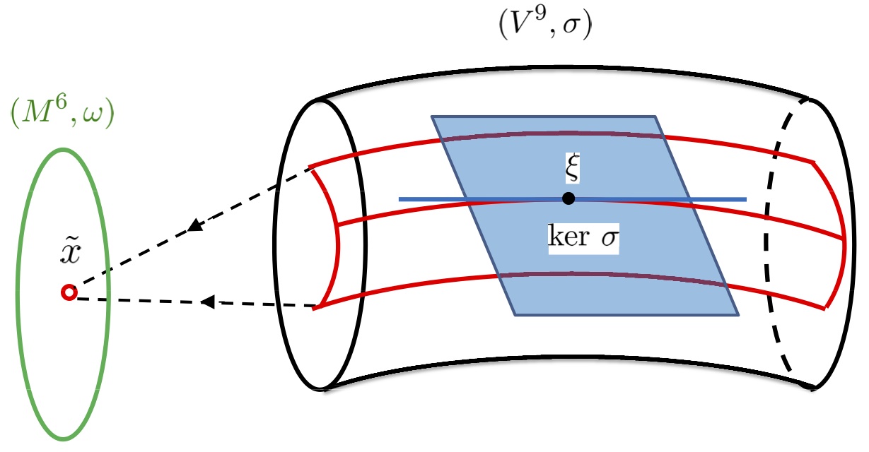
Figure 1: A free massless spinning particle has a 9-dimensional evolution space $V^{9}$; its dynamics is defined by a two-form $\sigma$ (see (3.5)), whose kernel, $\ker\sigma$, is $3$-dimensional. A motion is a leaf tangent to the latter. All points of a leaf can be reached by a Z-shift (also called a Wigner translation). The set of leaves forms the space of motions, $M^{6}$, whose points are $\tilde{x}=(\tilde{{\bm{x}}},\tilde{{\bm{p}}})$.

To obtain down-to-earth expressions, we put $R=({\bm{r}},t)$ where ${\bm{r}}$ and $t$ are the position and time coordinates in a chosen Lorentz frame. The two null-vectors are in turn $P=({\bm{p}},|{\bm{p}}|)$ and $J=({\bm{q}},-|{\bm{q}}|)$, where ${\bm{p}}$ and ${\bm{q}}$ are two (necessarily nonzero) $3$-vectors which satisfy ${\bm{p}}\cdot{\bm{q}}+|{\bm{p}}|\,|{\bm{q}}|=1$ by (3.1). In these terms we have

$$S_{ij}=\epsilon_{ijk}\,s^{k},\qquad{\bm{s}}=s\big{(}{\bm{p}}|{\bm{q}}|+{\bm{q}}|{\bm{p}}|\big{)},\qquad S_{j4}=s\big{(}{\bm{p}}\times{\bm{q}}\big{)}_{j}=\big{(}{\widehat{\bm{p}}}\times{\bm{s}}\big{)}_{j}.$$ (3.8)

We label each leaf of $\ker\sigma$ by picking a representative point in each of them in a way which is convenient for our purposes. To this end, we first observe that $\tau\to(R+\tau P,P,S)$ is an integral curve of $\ker\sigma$ for any given $(R,P,S)$, i.e., a particular “motion”. Next, shifting this curve by

$$Z=\big{(}\frac{{\widehat{\bm{p}}}}{|{\bm{p}}|}\times{\bm{s}},0\big{)}$$ (3.9)

yields another integral curve lying in the same leaf. Finally, taking $\tau=-t/|{\bm{p}}|$ yields the point which has zero time coordinate; this is the point that we choose. See Fig. 2 to illustrate our strategy.

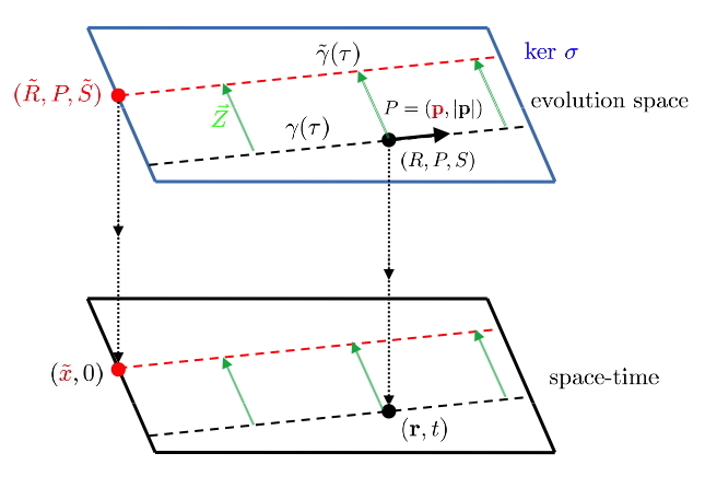
Figure 2: The spin of a motion tangent to the ($3$-dimensional) kernel of $\sigma$ can be enslaved by a suitable Z-shift. Choosing the point ${\color[rgb]{1,0,0}(\tilde{R},P,\tilde{S})}$ on the shifted curve with vanishing time coordinate, $\tilde{R}=(\tilde{{\bm{x}}},0)$, provides us with a coordinate ${\color[rgb]{1,0,0}\tilde{{\bm{x}}}}$ of the motion-sheet. The characteristic leaves in $V^{9}$ project to Minkowski space-time as $3$-planes orthogonal to the momentum: a massless spinning particle cannot be localized.

The corresponding point on the shifted curve has position $R=(\tilde{\bm{x}},0)$. Spin becomes enslaved to the linear $3$-momentum,

$$S_{j4}=0,\qquad{\bm{s}}=s\,{{\widehat{\bm{p}}}}.$$ (3.10)

An important observation which follows from (3.8) is that

$${\widehat{\bm{p}}}\cdot{\bm{s}}=s$$ (3.11)

in general, and not only in the enslaved case (3.10). It is thus not the length of the $3$ vector ${\bm{s}}$ but its projection along ${\widehat{\bm{p}}}$ which is a constant.

In terms of $(3+1)$-variables, $Z=({\bm{Z}},{\widehat{\bm{p}}}\cdot{\bm{Z}})$ the “Z-shift” (3.7) acts as

$${\bm{r}}\to{\bm{r}}+{\bm{Z}},\qquad t\to t+{\widehat{\bm{p}}}\cdot{\bm{Z}},\qquad{\bm{p}}\to{\bm{p}},\qquad{\bm{s}}\to{\bm{s}}+{\bm{p}}\times{\bm{Z}}.$$ (3.12)

Thus, in the free case, the freedom of Z-shifting allows us to eliminate the spin as an independent degree of freedom altogether and the entire leaf can be labelled by $\tilde{\bm{x}}$ and $\tilde{\bm{p}}={\bm{p}}\neq 0$ alone. The latter parametrize the space of motions $M^{6}=V^{9}/\ker\sigma$, which has therefore the topology of $T({\mathbb{R}}^{3}\!\setminus\!\{0\})$. Finally, the two-form $\sigma$ in (3.5) descends to the space of motions $M^{6}$ as the symplectic two-form (2.6), namely

$$\omega=d\tilde{p}_{i}\wedge d\tilde{x}^{i}-\frac{s}{2|\tilde{\bm{p}}|^{3}}\,\epsilon^{ijk}\,\tilde{p}_{i}\,d\tilde{p}_{j}\wedge d\tilde{p}_{k}.$$ (3.13)

Now we establish the Poincaré symmetry of the model. The Poincaré Lie algebra $\mathfrak{e}(3,1)$, spanned by the pairs $(\Lambda,\Gamma)$ where $\Lambda=(\Lambda_{\mu\nu})$ belongs to the Lorentz Lie algebra ${\mathfrak{so}}(3,1)$, and $\Gamma=(\Gamma^{\mu})$ is a translation in Minkowski space-time, ${\mathbb{R}}^{3,1}$, acts on $V^{9}$ by the lift of its action on Minkowski-space-time. This action on $V^{9}$ reads as follows

$$\delta R^{\mu}=\Lambda^{\mu}_{\,\nu}R^{\nu}+\Gamma^{\mu},\qquad\delta P^{\mu}=\Lambda^{\mu}_{\;\nu}P^{\nu},\qquad\delta S^{\mu\nu}=\Lambda^{\mu}_{\,\rho}S^{\rho\nu}-\Lambda^{\nu}_{\,\rho}S^{\rho\mu},$$ (3.14)

and clearly leaves the two-form (3.5) invariant. It is therefore a symmetry of the system, which descends to the space of motions $(M^{6},\omega)$. The associated Noetherian conserved quantities are

$$P^{\mu}=I^{\mu},\qquad M^{\mu\nu}=R^{\mu}P^{\nu}-R^{\nu}P^{\mu}+S^{\mu\nu},$$ (3.15)

which identifies the vector $P$ and the bi-vector $M$ as the conserved linear and angular momentum, respectively.

To get explicit formulas in a $(3+1)$-decomposition, we parametrize the Poincaré Lie algebra by $\Lambda_{ij}=\epsilon_{ijk}\,\omega^{k}$, $\Lambda_{i4}=\beta^{i}$ and $\Gamma=({\bm{\gamma}},\varepsilon)$, where $\mbox{\boldmath$\omega$},{\bm{\beta}},{\bm{\gamma}}\in\mathbb{R}^{3},\varepsilon\in\mathbb{R}$ are infinitesimal rotations, boosts and space- and time-translations, respectively. In terms of this decomposition, the infinitesimal Poincaré-action on $V^{9}$ is given, see (3.14) and (3.8), by

$$\left\{\begin{array}[]{lll}\delta{\bm{r}}&=&\mbox{\boldmath$\omega$}\times{\bm{r}}+{\bm{\beta}}{}t+{\bm{\gamma}},\\ \delta t&=&{\bm{\beta}}\cdot{\bm{r}}+\varepsilon,\\ \delta{\bm{p}}&=&\mbox{\boldmath$\omega$}\times{\bm{p}}+{\bm{\beta}}\,|{\bm{p}}|,\\ \delta{\bm{s}}&=&\mbox{\boldmath$\omega$}\times{\bm{s}}-{\bm{\beta}}\times({\widehat{\bm{p}}}\times{\bm{s}}),\end{array}\right.$$ (3.16)

and duly projects to Minkowski space-time as the natural one.

To write down the explicit form of the Poincaré momenta (3.15) we present the matrix $M=(M_{\mu\nu})$ (which belongs to the dual of the Lorentz algebra) as $M_{ij}=\epsilon_{ijk}\,\ell^{k}$ and $M_{j4}=g^{j}$ with $\bm{\ell}$ and ${\bm{g}}$ two $3$-vectors. In terms of the above $(3+1)$-parametrization we find

$$\left\{\begin{array}[]{lll}\bm{\ell}&=&{\bm{r}}\times{\bm{p}}\,+{\bm{s}},\\[4.0pt] {\bm{g}}&=&|{\bm{p}}|\,{\bm{r}}-{\bm{p}}t+{\widehat{\bm{p}}}\times{\bm{s}}.\end{array}\right.$$ (3.17)

Then the quantity

$$\tilde{\bm{x}}=\frac{{\bm{g}}}{|{\bm{p}}|}={\bm{r}}-{\widehat{\bm{p}}}\,{}t+\frac{{\widehat{\bm{p}}}}{|{\bm{p}}|}\times{\bm{s}}$$ (3.18)

is itself conserved. Working out the action of the full Poincaré Lie algebra (3.14) on the space of motions $(M^{6},\omega)$ provides us with

$$\left\{\begin{array}[]{lll}\delta\tilde{\bm{p}}&=&\mbox{\boldmath$\omega$}\times\tilde{\bm{p}}+\,|\tilde{\bm{p}}|\,{\bm{\beta}},\\[6.0pt] \delta\tilde{\bm{x}}&=&\mbox{\boldmath$\omega$}\times\tilde{\bm{x}}+s\,{\bm{\beta}}\times\displaystyle\frac{\tilde{\bm{p}}}{|\tilde{\bm{p}}|^{2}}-{\bm{\beta}}\cdot\tilde{\bm{x}}\,\displaystyle\frac{\tilde{\bm{p}}}{|\tilde{\bm{p}}|}+{\bm{\gamma}}-\varepsilon\,\frac{\tilde{\bm{p}}}{|\tilde{\bm{p}}|}.\end{array}\right.$$ (3.21)

The $10$-parameter vector field (3.21) leaves the free symplectic structure (3.13) invariant, i.e., it generates a family of symmetries, to which the symplectic Noether theorem SSD associates $10$ constants of the motion, namely

$$\left\{\begin{array}[]{lllll}\bm{\ell}&=&\tilde{\bm{x}}\times\tilde{\bm{p}}+s{{\widehat{\bm{p}}}}&&\hbox{angular momentum}\\ {\bm{g}}&=&|\tilde{\bm{p}}|\,\tilde{\bm{x}}&&\hbox{boost momentum}\\ {\bm{p}}&=&\tilde{\bm{p}}&&\hbox{linear momentum}\\ {\mathcal{E}}&=&|\tilde{\bm{p}}|&&\hbox{energy}\end{array}\right.$$ (3.22)

whose conservation follows also directly from the free equations of motions. Note that the two terms in the free angular momentum $\bm{\ell}$ are separately conserved .

The Poisson brackets of the quantities in (3.22) calculated using (3.13),

$$\begin{array}[]{lllll}\{\ell_{i},\ell_{j}\}=-\epsilon_{ij}^{k}\,\ell_{k},&\{\ell_{i},g_{j}\}=-\epsilon_{ij}^{k}\,g_{k},&\{\ell_{i},p_{j}\}=-\epsilon_{ij}^{k}\,p_{k},&\{\ell_{i},{\mathcal{E}}\}=0,&\\[6.0pt] \{g_{i},g_{j}\}=\epsilon_{ij}^{k}\,\ell_{k},&\{g_{i},p_{j}\}=-{\mathcal{E}}\,\delta_{ij},&\{g_{i},{\mathcal{E}}\}=-p_{i},&\{p_{i},p_{j}\}=0,&\{p_{i},{\mathcal{E}}\}=0,\end{array}$$ (3.23)

are those of the Poincaré Lie algebra $\mathfrak{e}(3,1)$, as expected. Calculating the Casimir invariants

$$m^{2}=-{\bm{p}}^{2}+{\mathcal{E}}^{2}=0,\qquad\bm{\ell}\cdot{\widehat{\bm{p}}}=s,$$ (3.24)

shows that the infinitesimal Poincaré symmetry we have just found is realized in the zero-mass and spin-$s$ representation.

The reason hidden behind all this is that the (connected) Poincaré group acts on the space of motions symplectically and transitively. Therefore $(M^{6},\omega)$ is a coadjoint orbit of the Poincaré group SSD . The symplectic form (3.13) is, in particular, Souriau’s $\#(17.145)$ in SSD . The $Z$-translations in equation (3.7), also identified as Wigner translations Wigner , belong to the stability subgroup, ${\rm SO}(2)\times{\mathbb{R}}^{3}$, of the Poincaré-action of a basepoint in the orbit.

So far, we have considered the infinitesimal action of the Poincaré Lie algebra. The construction allows us to work out the finite action of the connected (also called neutral) Poincaré Lie group on the space of motions $(M^{6},\omega)$. To that end it is enough to spell out its natural action

$$(R,I,J)\to(R^{\prime}=\mathcal{L}{}R+\mathcal{C},I^{\prime}=\mathcal{L}{}I,J^{\prime}=\mathcal{L}{}J)$$ (3.25)

with $\mathcal{L}\in{\rm SO}_{+}(3,1)$ and $\mathcal{C}\in{\mathbb{R}}^{3,1}$, integrating the infinitesimal action (3.14) on the evolution space $V^{9}$ introduced in (3.1). Parametrizing the connected Poincaré group by $A$ (rotation), ${\bm{b}}=b\,{\bm{u}}$ (boost in the direction ${\bm{u}}$), ${\bf c}$ (space-translation), and $e$ (time-translation), a tedious calculation summarized in Appendix C) yields the action $(\tilde{\bm{p}},\tilde{\bm{x}})\to(\tilde{\bm{p}}^{\prime},\tilde{\bm{x}}^{\prime})$, where

$$\left\{\begin{array}[]{lll}\tilde{\bm{p}}^{\prime}&=&{A}\,\tilde{\bm{p}}+(\gamma-1)\,({\bm{u}}\cdot{A}\,\tilde{\bm{p}})\,{\bm{u}}+\gamma\,|\tilde{\bm{p}}|\,{\bm{b}},\\[12.0pt] \tilde{\bm{x}}^{\prime}&=&\displaystyle\frac{1}{|\tilde{\bm{p}}|+{\bm{b}}\cdot{A}\,\tilde{\bm{p}}}\,\bigg{[}{\bm{b}}\times{A}\big{(}\tilde{\bm{x}}\times\tilde{\bm{p}}+s\,\displaystyle\frac{\tilde{\bm{p}}}{|\tilde{\bm{p}}|}\big{)}\\[12.0pt] &&+\,|\tilde{\bm{p}}|\,A\,\tilde{\bm{x}}+(\gamma-1)\,|\tilde{\bm{p}}|\,({\bm{u}}\cdot{A}\,\tilde{\bm{x}})\,{\bm{u}}\,-\,\gamma\,|\tilde{\bm{p}}|({\bm{b}}\cdot{A}\,\tilde{\bm{x}})\,{\bm{b}}+({\bm{b}}\cdot{A}\,\tilde{\bm{p}})\,{\bf c}\\[6.0pt] &&-\displaystyle\frac{e}{\gamma}\Big{(}{A}\,\tilde{\bm{p}}+(\gamma-1)\,({\bm{u}}\cdot{A}\,\tilde{\bm{p}})\,{\bm{u}}\Big{)}+\,|\tilde{\bm{p}}|\,({\bf c}-{\bm{b}}\,{e})\bigg{]},\end{array}\right.$$ (3.26)

with $\gamma=(1-|{\bm{b}}|^{2})^{-1/2}$ as usual; by keeping “tildes” we insist that our variables live on the space of motions (remember that $\tilde{\bm{p}}={\bm{p}}$ but $\tilde{\bm{x}}\neq{\bm{r}}$). This extends the infinitesimal action (3.21) to finite transformations.

In a Lorentz frame the trajectory labeled with $\tilde{\bm{x}}$ is given by (3.18), i.e.,

$$\tilde{\bm{x}}={\bm{r}}-{\widehat{\bm{p}}}\,{t}+\frac{{\widehat{\bm{p}}}}{|{\bm{p}}|}\times{\bm{s}},$$ (3.27)

which describes motion with the velocity of light, directed along ${\widehat{\bm{p}}}$. A Z-shift displaces the trajectory; starting, in particular, with “enslaved” spin, the latter is “unchained” and the trajectories one obtains fill a three-plane in $4$-space. However, it is easy to see using (3.16) that the right hand side of (3.27) remains invariant: the motion is not affected.

Intuitively, the freedom of Z-shifting is reminiscent of gauge freedom: it can always be performed at will; enslaving spin is in turn a sort of gauge fixing, allowing to interpret the result in terms of physical degrees of freedom alone.

We mention for completeness that the Poincaré symmetry of the massless spinning particle actually extends to an ${\mathfrak{so}}(4,2)$ conformal symmetry. See, e.g., CFH .

4 Poincaré symmetry of the free chiral model

Now we return to chiral fermions. Does the free system (1.1) admit a Poincaré symmetry ? For ${\bm{E}}={\bm{B}}=0$ the motions can be determined explicitly: the $\Theta$-term drops out from (2.1), yielding

$${\bm{x}}(t)=\tilde{\bm{x}}+{\widehat{\bm{p}}}{\,}t,\qquad{\bm{p}}(t)=\tilde{\bm{p}},$$ (4.1)

with $\tilde{\bm{x}}$ and $\tilde{\bm{p}}$ constant vectors (and ${\widehat{\bm{p}}}=\tilde{\bm{p}}/|\tilde{\bm{p}}|$). As explained in Sect. 2, the chiral space of motions $M^{6}=V^{7}/\ker\sigma$ can, therefore, be labeled by the constants of the motion

$$\tilde{\bm{x}}={\bm{x}}(t)-{\widehat{\bm{p}}}\,{t}\quad\hbox{and}\quad\tilde{\bm{p}}.$$ (4.2)

With the fields switched off, the two-form $\omega$ in (2.5) becomes precisely (3.13): the free chiral model has the same space of motions as that of the massless spinning particle with $s=1/2$, studied in Section 3.

Then, our strategy is to “import” the natural Poincaré symmetry of the massless spinning model to the chiral system through their common space of motions. From the identity of the space-of-motions coordinates $(\tilde{\bm{x}},\tilde{\bm{p}})$ we conclude that, in terms of the coordinates $({\bm{x}},{\bm{p}},t)$ on the chiral evolution space $V^{7}$, the strange-looking Poincaré action (3.21) (with $s=1/2$) becomes,

$$\left\{\begin{array}[]{lll}\delta{\bm{x}}&=&\mbox{\boldmath$\omega$}\times{\bm{x}}+\displaystyle{\bm{\beta}}\times\frac{{\widehat{\bm{p}}}}{2|{\bm{p}}|}+{\bm{\beta}}\,t+{\bm{\gamma}},\\ \delta{\bm{p}}&=&\mbox{\boldmath$\omega$}\times{\bm{p}}+|{\bm{p}}|\,{\bm{\beta}},\\ \delta{t}&=&{\bm{\beta}}\cdot{\bm{x}}+\varepsilon.\end{array}\right.$$ (4.6)

By construction, these vector fields generate the same Lie algebra as those in (3.21), namely the Poincaré algebra $\mathfrak{e}(3,1)$.

Equation (4.6) confirms the recently proposed action of the Lorentz subalgebra on chiral fermions ChenSon . The conserved quantities associated with the generators of the latter are, in particular,

$$\left\{\begin{array}[]{lll}\bm{\ell}&=&{\bm{x}}\times{\bm{p}}\,+{\frac{1}{2}}\,{\widehat{\bm{p}}},\\ {\bm{g}}&=&|{\bm{p}}|\,{\bm{x}}-{\bm{p}}{}t,\end{array}\right.$$ (4.9)

as it can be checked directly by showing that the infinitesimal rotations and boost generators in equation (4.6) Lie-transport the two-form $\sigma$ in (2.4)–(2.6), and then by calculating the associated Noetherian quantities.

We have thus established a twisted Poincaré symmetry of the free chiral system. We insist, however, that the action (4.6) is not the usual, natural one on Minkowski space-time. In fact, it is not an action on space-time at all, since it also involves the momentum variable ${\bm{p}}$; it is rather a sort of dynamical symmetry – but one for the free dynamics.

In conclusion, the chiral model admits a Poincaré symmetry, but, unlike for the massless spinning model, this symmetry does not act in the usual, natural way. It follows that ${\bm{x}}$ should not be considered as a bona fide position variable, because it does not transform under a boost as positions should : it labels a motion and is not a space coordinate. We contend that the well-founded position of our particle should rather be regarded as given by the three spatial coordinates, ${\bm{r}}$, relatively to a chosen Lorentz frame, of intrinsic space-time translations within the Poincaré group. From the identity of the space-of-motions coordinates $(\tilde{\bm{x}},\tilde{\bm{p}})$ we conclude in fact that the coordinates, ${\bm{x}}$, of the chiral particle are related to those, ${\bm{r}}$, of the massless Poincaré model according to

$${\bm{x}}={\bm{r}}+\frac{{\widehat{\bm{p}}}}{|{\bm{p}}|}\times{\bm{s}}\qquad\hbox{with}\qquad{\bm{s}}\cdot{\widehat{\bm{p}}}={\frac{1}{2}}.$$ (4.10)

The coordinates coincide, ${\bm{x}}={\bm{r}}$, only when spin is enslaved.

5 Coupling to an external electromagnetic field

Let us now cope with a number of procedures enabling us to couple our relativistic massless and spinning particle to an external electromagnetic field.

The conventional minimal coupling rule says that the $4$-momentum should be shifted by the $4$-potential as follows,

$$p_{\mu}\to p_{\mu}-eA_{\mu}.$$ (5.1)

This is not exactly what is proposed in (1.1), though: while the rule (5.1) is used for the $4$-momentum $({\bm{p}},h)$, the $3$-vector ${\bm{p}}$ in the Berry term $\Theta$ is not shifted. Remarkably, this “half-way-rule” is instead consistent with working with the same evolution space as for a free particle, but adding the electromagnetic field strength $F$ to the free two-form (3.5) SSD ,

$$\sigma\to\sigma+eF,$$ (5.2)

where $e$ is the electric charge of the system. This two-form is still closed, $d\sigma=0$, because $F$ is a closed two-form of Minkowski space-time.

The rules (5.1) and (5.2) are equivalent only in the spinless case. Then why should (5.2) be chosen? An argument in its favor comes form our personal experience of working in the plane, where it yielded an insight into Hall-type phenomena Peierls ; AnAn ; HMS ; ZH-chiral ; AHE ; OHE . In non-commutative mechanics in the plane, modifications of the principle (5.2) lead to unsatisfactory models, see HMS ; LSZ . The merits of (5.2) have been praised, for example, by Sternberg Sternberg78 . It is hence this scheme we will be using throughout this paper.

5.1 Minimal coupling of the massless spinning model

Applying the prescription (5.2) to the massless spinning model of Section 3 yields, on the evolution space $V^{9}$ in (3.4), the closed two-form

$$\sigma=-dP_{\mu}\wedge{}dR^{\mu}-\frac{1}{2s^{2}}\,d{S}^{\mu}_{\;\lambda}\wedge{S}^{\lambda}_{\;\rho}\,d{S}^{\rho}_{\;\mu}+\frac{e}{2}F_{\mu\nu}\,dR^{\mu}\wedge dR^{\nu}.$$ (5.3)

Then a lengthy calculation using the constraints in the definition (3.4) of $V^{9}$ shows that the equations of free motions (3.6) change to

$$\left\{\begin{array}[]{rcl}\dot{R}^{\mu}&=&P^{\mu}{}+\displaystyle\frac{S^{\mu\nu}{F}_{\nu\rho}P^{\rho}}{{\frac{1}{2}}{S\cdot{}F}},\\[8.0pt] \dot{P}^{\mu}&=&-eF^{\mu}_{\;\nu}\dot{R}^{\nu},\\[8.0pt] \dot{S}^{\mu\nu}&=&P^{\mu}\dot{R}^{\nu}-P^{\nu}\dot{R}^{\mu}.\end{array}\right.$$ (5.4)

assuming that ${S\cdot{}F}\equiv{S}_{\alpha\beta}F^{\alpha\beta}\neq 0$. The dimension of $\ker\sigma$ drops from $3$ to $1$: the spin-field coupling term in the velocity relation breaks the Z-shift-invariance. It follows that the spin degree can not now be eliminated and we are left with a $8$-dimensional space of motions (phase space, locally).

Let us now express the equations of motion (5.4) in terms of the $(3+1)$-decomposition we introduced in the previous section. Assuming, that

$$(a)\quad{\frac{1}{2}}{S\cdot{}F}\equiv{\frac{1}{2}}{S}_{\alpha\beta}F^{\alpha\beta}={\bm{s}}\cdot({\bm{B}}-{\widehat{\bm{p}}}\times{\bm{E}})\neq 0,\qquad(b)\quad{\widehat{\bm{p}}}\cdot{\bm{B}}\neq 0,$$ (5.5)

a strange cancellation takes place in the velocity relation in (5.4), which becomes

$$\dot{{\bm{r}}}=s|{\bm{p}}|\displaystyle\frac{{\bm{B}}-{\widehat{\bm{p}}}\times{\bm{E}}}{{\bm{s}}\cdot({\bm{B}}-{\widehat{\bm{p}}}\times{\bm{E}})},\qquad\dot{t}=s|{\bm{p}}|\displaystyle\frac{({\widehat{\bm{p}}}\cdot{\bm{B}})}{{\bm{s}}\cdot({\bm{B}}-{\widehat{\bm{p}}}\times{\bm{E}})}.$$ (5.6)

Condition (a), the analog of the nonvanishing of the effective mass, (2.8), will henceforth be assumed to hold.

Condition (b) in (5.5) requires that the momentum should not be perpendicular to the magnetic field. When it is not satisfied, then $\dot{t}=0$, so that, while the motion still takes place along a curve, it becomes instantaneous .

Let us assume that the regularity conditions (5.5) hold; then merging the two equations in (5.6) provides us with

$$\left\{\begin{array}[]{rcl}\displaystyle\frac{d{\bm{r}}}{dt}&=&\displaystyle\frac{{\bm{B}}-{\widehat{\bm{p}}}\times{\bm{E}}}{{\widehat{\bm{p}}}\cdot{\bm{B}}},\\[12.0pt] \displaystyle\frac{d{\bm{p}}}{dt}&=&e\big{(}{\bm{E}}+\displaystyle\frac{d{\bm{r}}}{dt}\times{\bm{B}}\big{)}=e\,\displaystyle\frac{{\bm{E}}\cdot{\bm{B}}}{{\widehat{\bm{p}}}\cdot{\bm{B}}}\,{\widehat{\bm{p}}},\\[12.0pt] \displaystyle\frac{d{{\bm{s}}}}{dt}&=&\displaystyle{\bm{p}}\times\frac{d{{\bm{r}}}}{dt}=\displaystyle\frac{{\bm{p}}\times{\bm{B}}}{{\widehat{\bm{p}}}\cdot{\bm{B}}}-\frac{{\bm{p}}\times({\widehat{\bm{p}}}\times{\bm{E}})}{{\widehat{\bm{p}}}\cdot{\bm{B}}}.\end{array}\right.$$ (5.7)

We insist on the rather unusual form of these equations. Firstly, the ${\widehat{\bm{p}}}$ one would have expected on the r.h.s. of the velocity relation cancels out; the electric charge drops out also. The dynamics of the momentum decouples from the spin as long as the latter does not vanish; also the scalar spin $s\neq 0$ disappears from all equations. Equations (5.7) imply that $d{\widehat{\bm{p}}}/dt=0$ so that the direction of ${\bm{p}}$ is unchanged during the motion. Spin is in fact not an independent variable, its (for space-time dynamics irrelevant) motion is entirely determined by the other dynamical data .

Let us put, for example, our massless but charged particle into crossed constant electric and magnetic fields like in the Hall effect, ${\bm{E}}=E\,\hat{{\bm{x}}}$, ${\bm{B}}=B\,\hat{{\bm{z}}}$, (say). Then ${\bm{p}}$ is itself a constant of the motion, and so is the angle $\vartheta$ between ${\bm{B}}$ and ${\bm{p}}$ (which cannot be $\pi/2$ for ${\bm{p}}\cdot{\bm{B}}\neq 0$). Let us assume for simplicity that the initial momentum lies in the $x$-$z$ plane.

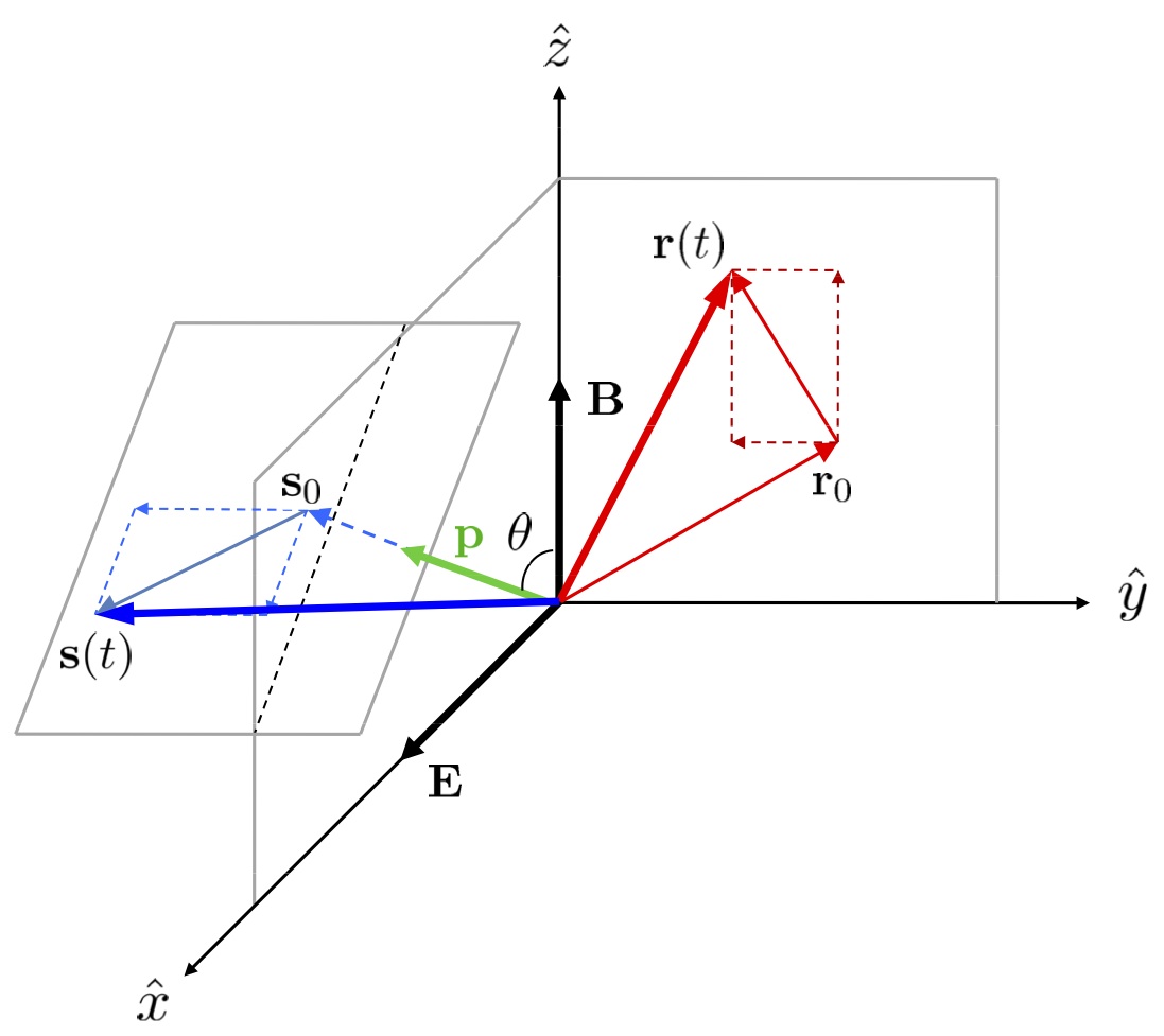
Figure 3: Motion in Hall-type electric and magnetic fields described by equation (5.8). The initial position, ${\bm{r}}_{0}$, is chosen in the $y$-$z$ plane, and the initial momentum and spin are chosen to be parallel and in the $x$-$z$ plane. Then, the spatial motion, ${\color[rgb]{1,0,0}{\bm{r}}}(t)$, is a combination of constant-velocity Hall drift perpendicularly to ${\bm{E}}$ and ${\bm{B}}$, combined with constant-velocity vertical drift. The momentum, ${\color[rgb]{0,1,0}{\bm{p}}}$, is conserved, but the spin, ${\color[rgb]{0,0,1}{\bm{s}}}(t)$, moves in a plane perpendicular to the momentum.

Then the equations of motion are solved by

$$\left\{\begin{array}[]{lll}{\bm{r}}(t)&=&\Big{(}(\cos\vartheta)^{-1}\,\hat{{\bm{z}}}-\displaystyle\frac{E}{B}\,\hat{{\bm{y}}}\Big{)}t+{\bm{r}}_{0},\\[4.0pt] {\bm{p}}(t)&=&{\bm{p}}_{0},\\[4.0pt] {\bm{s}}(t)&=&|{\bm{p}}|\Big{(}-\tan\vartheta\,\hat{{\bm{y}}}+\displaystyle\frac{E}{B}\big{(}\cos\vartheta\,\hat{{\bm{x}}}-\sin\vartheta\,\hat{{\bm{z}}})\Big{)}\,t+{\bm{s}}_{0}.\end{array}\right.$$ (5.8)

Thus, in addition to a constant-speed vertical motion, the “particle” also drifts perpendicularly to the electric field with Hall velocity ${E}/{B}.$ The spin vector follows an even more curious motion perpendicularly to ${\widehat{\bm{p}}}$ so that its projection on ${\widehat{\bm{p}}}$ remains a constant, ${\bm{s}}(t)\cdot{\widehat{\bm{p}}}={\bm{s}}_{0}\cdot{\widehat{\bm{p}}}.$ Thus while spin is decoupled, it can not consistently be enslaved as in (3.10) since ${\bm{s}}$ and ${\widehat{\bm{p}}}$ do not remain parallel even if we start with a such initial condition, see Fig. 3. Note that $S.F=2sB\cos\vartheta$ for such a motion and the system is regular therefore when $\vartheta\neq\pi/2$.

The velocity is superluminal ($|d{\bm{r}}/dt|>1$) and diverges as $\vartheta\to\pi/2$; for ${\widehat{\bm{p}}}\cdot{\bm{B}}=0$ we get instantaneous motions, i.e. with infinite velocity, parallel to the $z$ axis. This is in fact a general property, as seen from (5.4), because $\dot{R}_{\mu}\dot{R}^{\mu}<0$, the $4$-vector $(S^{\mu\nu}{F}_{\nu\rho}P^{\rho})$ being space-like.

5.2 Anomalous coupling

The model of Section 5.1 is not completely satisfactory, and now we generalize our minimal scheme. Our clue is to allow the “mass-square” $P_{\mu}{P}^{\mu}$ to depend on the coupling of spin to the electromagnetic field as suggested in Souriau74 ; Duval75 , i.e.,

$$P_{\mu}{P}^{\mu}=-\frac{eg}{2}\,S\cdot{}F,$$ (5.9)

where we used once again the shorthand $S\cdot{}F\equiv{}S_{\alpha\beta}F^{\alpha\beta}$, cf. (5.5). The real constant $g$ will be interpreted as the gyromagnetic ratio . Generalizing the previous relation $P=I$ as

$$P^{\mu}=I^{\mu}+\frac{eg}{4}\,(S\cdot{}F)J^{\mu},$$ (5.10)

where $I$ and $J$ are still as in (3.1), helps us to implement the equation of state (5.9). The condition $S_{\mu\nu}P^{\nu}=0$ is also automatically satisfied.

Hence we introduce the novel evolution space

$$\widetilde{V}^{9}=\left\{P,R\in{\mathbb{R}}^{3,1},S\in{\mathfrak{o}}(3,1)\,\Big{|}\,P_{\mu}{}P^{\mu}=-\frac{eg}{2}\,S\cdot{}F,\;S_{\mu\nu}P^{\nu}=0,\;{\frac{1}{2}}{S}_{\mu\nu}{S}^{\mu\nu}=s^{2}\right\},\quad$$ (5.11)

endowed with the closed two-form,

$$\sigma=-dP_{\mu}\wedge{}dR^{\mu}-\frac{1}{2s^{2}}\,d{S}^{\mu}_{\lambda}\wedge{S}^{\lambda}_{\rho}\,d{S}^{\rho}_{\mu}+{\frac{1}{2}}{}eF_{\mu\nu}\,dR^{\mu}\wedge{}dR^{\nu}.$$ (5.12)

Note that (5.12) is formally the same as (5.3) up to the mass-shell constraint (5.9).

Some more effort is needed to work our the new equations of motion from the kernel of $\sigma$ using the constraints which define $\widetilde{V}^{9}$. We find that a curve $(R(\tau),P(\tau),S(\tau))$ is tangent to $\ker\sigma$ in (5.12) iff

$$\left\{\begin{array}[]{rcl}\dot{R}^{\mu}&=&\displaystyle P^{\mu}-\frac{1}{(g+1)}\frac{1}{S_{\alpha\beta}F^{\alpha\beta}}\Big{[}(g-2)\,{S}^{\mu\nu}F_{\nu\rho}{}P^{\rho}-g\,{S}^{\mu\nu}{\partial}_{\nu}F_{\rho\sigma}\,{S}^{\rho\sigma}\Big{]},\\[12.0pt] \dot{P}^{\mu}&=&\displaystyle-eF^{\mu}_{\;\nu}\,\dot{R}^{\nu}-\frac{eg}{4}\,{\partial}^{\mu}F_{\rho\sigma}\,{S}^{\rho\sigma},\\[12.0pt] \dot{S}^{\mu\nu}&=&\displaystyle P^{\mu}\dot{R}^{\nu}-P^{\nu}\dot{R}^{\mu}+\frac{eg}{2}\,\Big{[}{S}^{\mu}_{\;\rho}\,F^{\rho\nu}-{S}^{\nu}_{\;\rho}\,F^{\rho\mu}\Big{]}.\end{array}\right.$$ (5.13)

These equations, which reduce to (5.3) for $g=0$, constitute the zero-rest-mass counterparts of the celebrated Bargmann-Michel-Telegdi equations for massive relativistic particles BMT , as well as $4$ dimensional analogs of “exotic” anyons in the plane AnAn . In the normal case, $g=2$, resulting from the Dirac equation Duval75 , the previously considered anomalous velocity is canceled but there arises a new, Stern - Gerlach-type contribution involving the derivative of the external electromagnetic field. Thus, an anomalous velocity term shows up for any value of the gyromagnetic ratio $g$.

Now we turn to a $(3+1)$-decomposition. Things behave as before, up to some subtle differences. Firstly, we have

$$R=({\bm{r}},t),\qquad P=({\bm{p}},{\mathcal{E}}),\qquad S_{j4}=\left(\frac{{\bm{p}}}{{\mathcal{E}}}\times{\bm{s}}\right)_{j},$$ (5.14)

where the spin tensor is still defined as in (3.2), but the new dispersion relation generalizes (3.22) , namely

$${\mathcal{E}}=\sqrt{|{\bm{p}}|^{2}-\frac{eg}{2}S\cdot{}F\,}\,.$$ (5.15)

Decomposing the electromagnetic field into its electric and magnetic components, the quantity (5.5) (a) is generalized to

$${\frac{1}{2}}S\cdot{}F={\bm{s}}\cdot\left({\bm{B}}-\frac{{\bm{p}}}{{\mathcal{E}}}\times{\bm{E}}\right).$$ (5.16)

Then a rather tedious calculation yields the following $(3+1)$-form of the equations of motion (5.13), namely

$$\left\{\begin{array}[]{rcl}\dot{{\bm{r}}}&=&\displaystyle\frac{3g}{2(g+1)}\,{\bm{p}}-\left(\frac{g-2}{g+1}\right)\left[\displaystyle\frac{{\bm{s}}\cdot{\bm{p}}}{S\cdot{}F}\left({\bm{B}}-\frac{{\bm{p}}}{{\mathcal{E}}}\times{\bm{E}}\right)-\frac{eg}{2}{\bm{E}}\times\frac{{\bm{s}}}{{\mathcal{E}}}\right]\\[12.0pt] &&-\,\displaystyle\frac{g}{2(g+1)S\cdot{}F}\,\Big{(}{\bm{s}}\times(S\cdot{\bm{D}}{F})-\frac{{\bm{p}}}{{\mathcal{E}}}\times{\bm{s}}\,(S\cdot{}D_{t}F)\Big{)},\\[20.0pt] \dot{t}&=&\displaystyle\frac{g}{2(g+1){\mathcal{E}}}\big{(}3|{\bm{p}}|^{2}-(g+1)eS\cdot{}F\big{)}-\left(\frac{g-2}{g+1}\right)\frac{1}{{{\mathcal{E}}}\,S\cdot{}F}\,({{\bm{p}}\cdot{\bm{B}}})({\bm{s}}\cdot{\bm{p}})\\[12.0pt] &&+\displaystyle\frac{eg(g-2)}{2(g+1){{\mathcal{E}}}^{2}}\,{\bm{s}}\cdot({\bm{p}}\times{\bm{E}})-\displaystyle\frac{g}{(g+1)}\frac{1}{{\mathcal{E}}\,S\cdot{}F}({\bm{p}}\times{{\bm{s}}})\cdot(S\cdot{\bm{D}}{F}),\\[20.0pt] \dot{{\bm{p}}}&=&e\big{(}{\bm{E}}\,\dot{t}+\dot{{\bm{r}}}\times{\bm{B}}\big{)}+\displaystyle\frac{eg}{4}S\cdot{\bm{D}}{F},\\[20.0pt] \dot{{\bm{s}}}&=&\displaystyle{\bm{p}}\times\dot{{\bm{r}}}+\displaystyle\frac{eg}{2}\left(\left(\frac{{\bm{p}}}{{\mathcal{E}}}\times{\bm{s}}\right)\times{\bm{E}}+{\bm{s}}\times{\bm{B}}\right),\\ \end{array}\right.$$ (5.17)

where we introduced the new shorthands

$$S\cdot{}D_{j}F=2{\bm{s}}\cdot\left({\partial}_{j}{\bm{B}}-\frac{{\bm{p}}}{{\mathcal{E}}}\times{\partial}_{j}{\bm{E}}\right),\qquad S\cdot{}D_{t}F=2{\bm{s}}\cdot\left({\partial}_{t}{\bm{B}}-\frac{{\bm{p}}}{{\mathcal{E}}}\times{\partial}_{t}{\bm{E}}\right).$$ (5.18)

When $g=0$ we recover (5.7).

To gain more insight, we consider the case $g=2$ and assume that the external fields are constant . Then the field-derivative terms drop out as does also the anomalous velocity term , and the complicated system (5.17) simplifies to one reminiscent of a massive relativistic particle,

$$(g=2)\qquad\left\{\begin{array}[]{cll}{\mathcal{E}}\,\displaystyle\frac{d{\bm{r}}}{dt}&=&\displaystyle{{\bm{p}}},\\[12.0pt] \displaystyle\frac{d{\bm{p}}}{dt}&=&e\left({\bm{E}}+\displaystyle\frac{{\bm{p}}}{{\mathcal{E}}}\times{\bm{B}}\right),\\[12.0pt] \displaystyle\frac{d{\bm{s}}}{dt}&=&\displaystyle\frac{e}{{\mathcal{E}}}\left(\big{(}\displaystyle\frac{{\bm{p}}}{{\mathcal{E}}}\times{\bm{s}}\big{)}\times{\bm{E}}+\displaystyle{{\bm{s}}}\times{\bm{B}}\right),\end{array}\right.$$ (5.19)

assuming that ${\mathcal{E}}\neq 0$, which acts as a sort of effective mass, is real. (Recall that ${\bm{p}}\neq 0$ implies that ${\mathcal{E}}$ can not vanish).

In a pure magnetic field momentum and spin satisfy equations of identical form,

$$\frac{d{\bm{p}}}{dt}=\frac{e}{{\mathcal{E}}}\,{\bm{p}}\times{\bm{B}},\qquad\frac{d{\bm{s}}}{dt}=\frac{e}{{\mathcal{E}}}\,{\bm{s}}\times{\bm{B}}.$$ (5.20)

Thus

$$\left\{\begin{array}[]{cc}|{\bm{p}}|=\mathop{\rm const}\nolimits\neq 0,&{\bm{p}}\cdot{\bm{B}}=\mathop{\rm const}\nolimits,\\[4.0pt] |{\bm{s}}|=\mathop{\rm const}\nolimits\neq 0,&{\bm{s}}\cdot{\bm{B}}=\mathop{\rm const}\nolimits,\end{array}\right.\quad\implies\quad\left\{\begin{array}[]{cll}p_{z}&=&\mathop{\rm const}\nolimits,\qquad s_{z}=\mathop{\rm const}\nolimits,\\[4.0pt] {\mathcal{E}}&=&\sqrt{|{\bm{p}}|^{2}-e{\bm{s}}\cdot{\bm{B}}}=\mathop{\rm const}\nolimits.\end{array}\right.$$ (5.21)

Choosing the $z$ axis in the direction of the magnetic field, ${\bm{B}}=B\hat{{\bm{z}}}$, for example, the momentum and spin vectors precess and the position spirals around the $z$ axis with common angular velocity $\omega=-eB/{\mathcal{E}}$,

$${\bm{p}}(t)=(p_{0}e^{-i(eB/{\mathcal{E}})t},p_{z}),\;{\bm{s}}(t)=(s_{0}e^{-i(eB/{\mathcal{E}})t},s_{z}),\;{\bm{r}}(t)=\Big{(}\frac{ip_{0}}{eB}\,e^{-i(eB/{\mathcal{E}})t},\,\frac{p_{z}}{{\mathcal{E}}}t\Big{)}+{\bm{r}}_{0},\;$$ (5.22)

where $p_{0}=p_{x}+ip_{y},\,s_{0}=s_{x}+is_{y}$, cf. Fig. 4. It is worth noting that for weak fields and pure magnetic field, and ${\bm{s}}={\frac{1}{2}}{\widehat{\bm{p}}}$ ,

$${\mathcal{E}}\approx|{\bm{p}}|-\frac{eg}{4}S\cdot{}F=|{\bm{p}}|-e\,\frac{{\widehat{\bm{p}}}\cdot{\bm{B}}}{2|{\bm{p}}|},$$ (5.23)

which is the modified dispersion relation proposed in SonYama2 ; ChenSon ; Manuel .

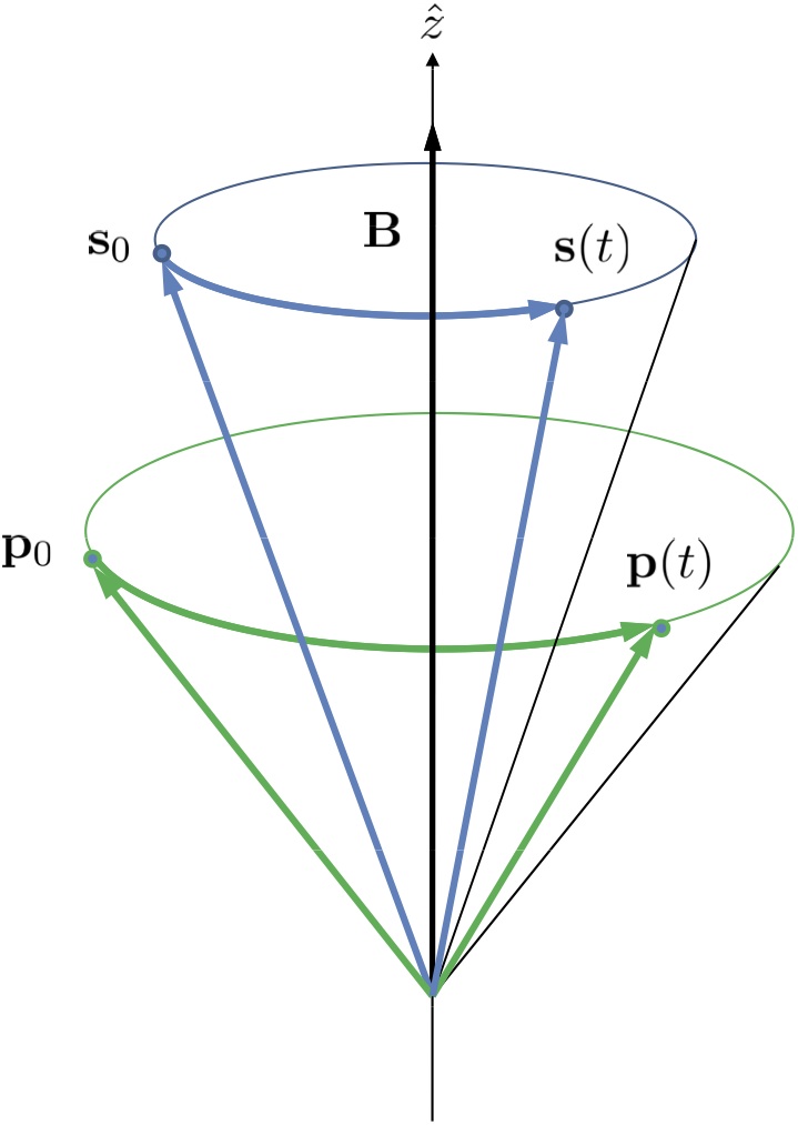
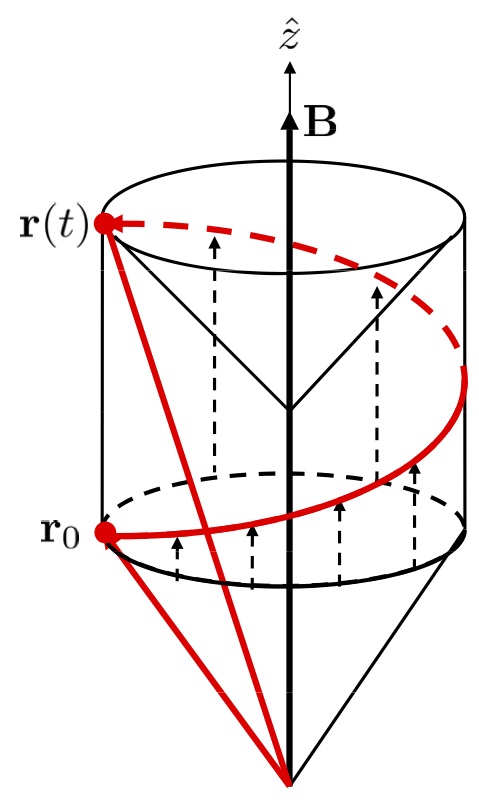
(a)                                                 (b)

Figure 4: (a) Motion in pure constant magnetic field ${\bm{B}}$. Both momentum ${\color[rgb]{0,1,0}{\bm{p}}}(t)$ and spin ${\color[rgb]{0,0,1}{\bm{s}}}(t)$ precess, with identical angular velocity, around the ${\bm{B}}$ direction, cf. eqn (5.22). (b) The position ${\color[rgb]{1,0,0}{\bm{r}}}(t)$ spirals on a cylinder around the ${\bm{B}}$-axis, obtained by combining precession with the vertical drift of the supporting cone itself.

By eqns (5.22) the direction of the rotation is reversed if the sign of the electric charge $e$ is reversed, whereas the direction of the vertical propagation is unchanged. As to chirality, when the sign of spin is reversed, eqns (5.22) yield similar spiraling motions, rotating and drifting in the same directions but with different angular velocities, namely with

$$\omega_{\pm}=-\frac{eB}{{\mathcal{E}}_{\pm}}=-\frac{eB}{\sqrt{|{\bm{p}}|^{2}\mp{e}{\widehat{\bm{p}}}\cdot{\bm{B}}}}\approx-\frac{eB}{|{\bm{p}}|}\left(1\pm\frac{e{\widehat{\bm{p}}}\cdot{\bm{B}}}{2|{\bm{p}}|}\right),$$ (5.24)

assuming that the magnetic field is weak.

In the purely magnetic case, enslavement (3.10) can be consistently required. However, this is manifestly not so in the presence of an electric field : the independent spin degree of freedom can not be switched off if ${\bm{E}}\neq 0$.

6 Conclusion

In this paper we have shown that the semiclassical chiral fermion model, much discussed in recent times in connection with the chiral magnetic and chiral vortical effects SonYama1 ; hadrons ; SonYama2 ; Stephanov ; ChenWang ; Dunne ; Stone ; Chen2013 ; ChenSon , can, in the free case, be related to the zero mass and spin-$1/2$ particle model of SSD . The latter carries a natural Poincaré symmetry that can be exported to chiral fermions using the above relation.

We obtain, in particular, Lorentz boosts as proposed recently ChenSon . One could argue that this is what one would expect for a relativistic theory; we would like to stress, however, that this action is not the usual, natural one on ordinary space-time — on the contrary, it resembles a dynamical symmetry in that it also involves the momentum. We contend that the variable ${\bm{x}}$, viewed commonly as position, does not transform correctly under a boost; it is rather our ${\bm{r}}$, which is the bona fide position coordinate studied in Sections 3 and 4. The situation is reminiscent of that of Newton-Wigner coordinates, familiar for the Dirac equation.

Our model is similar to but different from those proposed in SonYama1 ; hadrons ; Stephanov ; SonYama2 ; ChenWang ; Dunne ; Stone ; Chen2013 ; ChenSon ; Manuel  : while the usual chiral model (1.1) has no independent spin variable, ours has additional degrees of freedom associated with unchained spin and instrumental for having a natural Poincaré action. These additional degrees of freedom do not influence the free dynamics, though, as they can be eliminated by enslaving the spin to the momentum, using the additional symmetry referred to as Wigner (-Souriau) translations Wigner ; Penrose67 ; SSD ; NewStone ; WS .

The models become even more different when coupled to an external field : the standard chiral models have a $6$-dimensional phase space, whereas ours has, in the coupled case, $8$ dimensions. Also the motions appear rather different in the two frameworks. The difference comes from choosing the physically relevant position coordinate: ${\bm{x}}$ in the chiral model and ${\bm{r}}$ in the one we propose here. The question is not purely academic, since the coupling to a field is expressed precisely in terms of the position.

The difference between the theories originates in that in the usual approach SonYama1 ; Stephanov ; Stone ; Dunne ; SonYama2 ; hadrons ; ChenWang ; Chen2013 ; ChenSon ; Manuel ; NewStone ; WS they are derived from some widely accepted and physically trusted theory like the Dirac equation, transport theory, fluid dynamics, etc, while we build ours from the principles of Souriau’s mechanics, based on group theory, cf. SSD ; Souriau74 .

We present our investigations in symplectic, instead of usual variational terms. Although the two frameworks are essentially equivalent SSD ; VarSpin , the symplectic one is better adapted to study degenerate systems as in the free case. An alternative point of view is presented in WS .

Non-Abelian generalization could also be considered along the lines discussed in DuvalAix .

A Appendix : Souriau’s mechanics as generalized variational calculus

In the framework of SSD the dynamics is determined by a closed two-form $\sigma$ of constant rank defined on some evolution space $V$; the motions, described by curves or by surfaces of $V$, are the so-called “characteristic leaves”, tangent to the kernel, $\ker\sigma$, of the two-form $\sigma$.

To explain how this comes about, we consider a particle described by a Lagrangian on phase space of which (1.1) is an example that will serve as an illustration. Denoting the phase space variables ${\bm{x}}$ and ${\bm{p}}$ collectively by $\xi=(\xi^{\alpha})$, the Lagrangian in (1.1) is of the form $u_{\alpha}\dot{\xi}^{\alpha}-h(\xi)$ and the associated variational equations are

$$\omega_{\alpha\beta}\dot{\xi}^{\beta}={\partial}_{\alpha}{h},\qquad\hbox{where}\qquad\omega_{\alpha\beta}={\partial}_{\alpha}{u}_{\beta}-{\partial}_{\beta}{u}_{\alpha}.$$ (A.1)

We note en passant that if the matrix $(\omega_{\alpha\beta})$ is regular, then multiplying (A.1) with the inverse matrix would yield Hamilton’s equations.

A next step is to extend the $6$-dimensional phase space into the $7$-dimensional evolution space $V^{7}$ described by triples $y=({\bm{x}},{\bm{p}},t)$ and unify the two-form $\omega={\frac{1}{2}}\omega_{\alpha\beta}d\xi^{\alpha}\wedge d\xi^{\beta}$ with the Hamiltonian into the two-form

$$\sigma=\omega-dh\wedge dt.$$ (A.2)

Then the equations of motion (A.1) become finally

$$\sigma(\dot{y},\,\cdot\,)=0,$$ (A.3)

expressing that the velocity, $\dot{y}$, of the motion unfolded into the evolution space belongs to $\ker{\sigma}$, see Fig. 5.

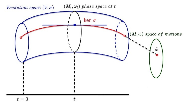
Figure 5: A motion is described, in the evolution space $V$, by a submanifold, which is tangent to the kernel of a closed two-form, $\sigma$, of constant rank. The space of motions is the symplectic manifold, $(M,\omega)$, obtained from $(V,\sigma)$ by factoring out these characteristic submanifolds. A phase space at time $t$ is a section of the evolution space for a fixed value of $t$, and provides a local chart of the space of motions.

More generally, we can consider an evolution space $V$ of dimension $d$, endowed with a closed two-form $\sigma$ of constant rank; let the kernel of $\sigma$ be an $r$-dimensional vector space. Then general theorems guarantee that $\ker{\sigma}$ is tangent, at each point, to an $r$-dimensional submanifold called a characteristic leaf of $\sigma$; the latter can be viewed as solution of a generalized variational problem.

Factoring out the characteristic leaves provides us with a symplectic manifold $(M,\omega)$ of dimension $2n=d-r$, called the space of motions, which can be regarded as an abstract substitute for the phase space. For further details the reader is invited to consult, e.g., SSD ; VarSpin .

We just mention that a symmetry is a transformation of the evolution space $V$ which preserves its two-form $\sigma$. The relation between symmetries and conservation laws is established by the symplectic form of Noether’s theorem. Conversely, the space of motions of classical systems with a given symmetry can be constructed, under suitable conditions, by group theoretical considerations SSD .

B Appendix : Massless, spinning relativistic particle models

We recall, here, the model of massless, spinning particle dwelling in Minkowski space-time, as spelled out in SSD , Section (14.29). The space of motions (or of classical states) of a free relativistic particle is a homogeneous symplectic manifold of the Poincaré group, $\mathrm{E}(3,1)$. These coadjoint orbits are known and classified; those with zero mass, and nonzero spin are constructed as follows.

For convenience we deal with the neutral Poincaré group $G=\mathrm{SE}_{+}(3,1)$ whose elements are pairs $g=(\mathcal{L},\mathcal{C})$ with $\mathcal{L}\in{\rm SO}_{+}(3,1)$, and $\mathcal{C}\in\mathbb{R}^{3,1}$, a space-time translation. Every element of the dual $\mathfrak{e}(3,1)^{*}$ of the Lie algebra, $\mathfrak{e}(3,1)$, of $G$ is a pair $\mu=(M,P)$ with $M\in{\mathfrak{so}}(3,1)$, the Lorentz momentum, and $P\in\mathbb{R}^{3,1}$, the linear momentum. The pairing between these spaces is given by $\mu\cdot{}Z={\frac{1}{2}}{}M_{\mu\nu}\Lambda^{\mu\nu}-P_{\mu}\Gamma^{\mu}$ with $Z=(\Lambda,\Gamma)\in\mathfrak{e}(3,1)$.

We will deal with oriented and time-oriented Lorentz frames $E=(I,J,K,L)$ of Minkowski space-time such that the only nonzero scalar products are $I_{\mu}{}J^{\mu}=K_{\mu}{}K^{\mu}=L_{\mu}{}L^{\mu}=-1$, with $I$ (null) future-pointing. It is useful to identify those frames with the neutral Lorentz group via $E=\mathcal{L}{}E_{0}$, where $E_{0}$ is some fixed frame, as well as space-time translations, $\mathcal{C}$, with Minkowskian events, $R$.

Picking then a fixed Poincaré-momentum $\mu_{0}=(M_{0},P_{0})$ such that $M_{0}=sI_{0}\times{}J_{0}$ (the cross-product of $I_{0}$ and $J_{0}$, i.e., $(M_{0})_{\mu\nu}=-s\,\epsilon_{\mu\nu\rho\sigma}\,I_{0}^{\rho}{}J_{0}^{\sigma}$) with $s>0$ interpreted as the classical spin, and $P_{0}=I_{0}$, we may define the one-form

$$\alpha=\mu_{0}\cdot g^{-1}dg$$ (B.1)

on $G$. Then, as a general result, the two-form

$$\sigma=d\alpha$$ (B.2)

descends to the coadjoint orbit $M=G/G_{\mu_{0}}$ as its canonical symplectic form; the leaves generated by the stabilizer $G_{\mu_{0}}$ of $\mu_{0}$ are interpreted as the motions of our (free) particle and integrate, by construction, the null distribution, $\ker\sigma$, on $(G,\sigma)$. These leaves project down to space-time as the worldsheets of our particle.

In the case under study the one-form (B.1) of $G$ reads

$$\alpha=-I_{\mu}\,dR^{\mu}+sK_{\mu}\,dL^{\mu},$$ (B.3)

whereas its derivative (B.2) descends to the evolution space $V^{9}=G/{\rm SO}(2)$ in (3.1), the ${\rm SO}(2)$-action on $G$ being $(I,J,K,L,R)\to(I,J,K\cos\theta+L\sin\theta,-K\sin\theta+L\cos\theta,R)$. This two-form, still denoted by $\sigma$ with a slight abuse of notation, is finally given by (3.5) where we have put $P=I$ for the four-momentum, and $S=sI\times{}J$ for the spin tensor.

C Appendix : Finite coadjoint action of the Poincaré group

We recall that a Lorentz transformation of $\mathbb{R}^{3,1}$ is of the form

$$\mathcal{L}=\exp\left(\begin{array}[]{cc}0&\alpha{\bm{u}}\\[4.0pt] \alpha{\bm{u}}^{T}&0\end{array}\right).\left(\begin{array}[]{cc}A&0\\[4.0pt] 0&1\end{array}\right)\in{\rm SO}_{+}(3,1),$$ (C.1)

where $\alpha\in\mathbb{R}$ is the rapidity and ${\bm{u}}\in{}S^{2}$ the direction of the boost, ${\bm{b}}=\tanh\alpha\,{\bm{u}}$, and $A\in{\rm SO}(3)$; we put $\gamma=\cosh\alpha=(1-|{\bm{b}}|^{2})^{-{\frac{1}{2}}}$. Using the shorthand $B=(B^{i}_{j})=(\delta^{i}_{j}+(\gamma-1)u^{i}\,u_{j})$, an element of the connected (also called neutral) Poincaré group is of the form

$$g=\left(\begin{array}[]{ccc}BA&\gamma\,{\bm{b}}&{\bf c}\\[4.0pt] \gamma{\bm{b}}^{T}A&\gamma&e\\[4.0pt] 0&0&1\end{array}\right)\in\mathrm{SE}_{+}(3,1),$$ (C.2)

where ${\bf c}\in\mathbb{R}^{3}$ is a space-translation, and $e\in\mathbb{R}$ a time-translation. The Lie algebra of the Poincaré group is therefore spanned by the matrices

$$Z=\left(\begin{array}[]{ccc}\widetilde{\mbox{\boldmath$\omega$}}&{\bm{\beta}}&{\bm{\gamma}}\\[6.0pt] {\bm{\beta}}^{T}&0&\varepsilon\\[6.0pt] 0&0&0\end{array}\right)\in\mathfrak{e}(3,1)$$ (C.3)

where $\widetilde{\mbox{\boldmath$\omega$}}\in{\mathfrak{so}}(3)$ is identified with $\mbox{\boldmath$\omega$}\in\mathbb{R}^{3}$, also ${\bm{\beta}},{\bm{\gamma}}\in\mathbb{R}^{3}$ and $\varepsilon\in\mathbb{R}$. Then the adjoint action $Z\to{}Z^{\prime}=(\mbox{\boldmath$\omega$}^{\prime},{\bm{\beta}}^{\prime},{\bm{\gamma}}^{\prime},\epsilon^{\prime})=\mathrm{Ad}(g^{-1})Z$ reads

$$\mbox{\boldmath$\omega$}^{\prime} = A^{T}\big{(}\gamma\mbox{\boldmath$\omega$}-(\gamma-1){\bm{u}}({\bm{u}}\cdot\mbox{\boldmath$\omega$})+\gamma{\bm{b}}\times{}B{\bm{\beta}}\big{)}$$ (C.4)

$${\bm{\beta}}^{\prime} = A^{T}\big{(}\gamma{}A(\mbox{\boldmath$\omega$}\times{\bm{b}})-\gamma^{2}{\bm{b}}({\bm{b}}\cdot{\bm{\beta}})+\gamma{}A{\bm{\beta}}\big{)}$$ (C.5)

$${\bm{\gamma}}^{\prime} = A^{T}\big{(}A(\mbox{\boldmath$\omega$}\times{\bf c})-\gamma{\bm{b}}({\bf c}\cdot{\bm{\beta}})+A{\bm{\beta}}{}\,e+A{\bm{\gamma}}-\gamma{\bm{b}}\,\varepsilon\big{)}$$ (C.6)

$$\varepsilon^{\prime} = \gamma\big{(}({\bm{b}}\times{\bf c})\cdot\mbox{\boldmath$\omega$}+{\bm{\beta}}\cdot{\bf c}-({\bm{b}}\cdot{\bm{\beta}}){}\,e-{\bm{b}}\cdot{\bm{\gamma}}+\varepsilon\big{)}.$$ (C.7)

Denoting by $\mu=(\bm{\ell},{\bm{g}},{\bm{p}},{\mathcal{E}})$ a “moment” in $\mathfrak{e}(3,1)^{*}$ where $\mu\cdot{}Z=\bm{\ell}\cdot\mbox{\boldmath$\omega$}-{\bm{g}}\cdot{\bm{\beta}}+{\bm{p}}\cdot{\bm{\gamma}}-{\mathcal{E}}\,\varepsilon$, we then find the coadjoint representation $\mu\to\mu^{\prime}=\mu\circ\mathrm{Ad}(g^{-1})$ where

$$\bm{\ell}^{\prime} = \gamma{}A\bm{\ell}-(\gamma-1)(\,{\bm{u}}{\cdot}A\bm{\ell}){\bm{u}}-\gamma{\bm{b}}\times{}A{\bm{g}}+{\bf c}\times{}A{\bm{p}}$$ (C.8)

$$-\gamma{{\mathcal{E}}}\,{\bm{b}}\times{\bf c}{}-(\gamma-1)\,({\bm{u}}{\cdot}A{\bm{p}})\,{\bm{u}}\times{\bf c}$$

$${\bm{g}}^{\prime} = \gamma{\bm{b}}\times{}A\bm{\ell}+\gamma{}A{\bm{g}}-(\gamma-1)\big{(}{\bm{u}}{\cdot}A({\bm{g}}+{\bm{p}}{}e)\big{)}\,{\bm{u}}+\gamma({\bm{b}}{\cdot}A{\bm{p}})\,{\bf c}$$ (C.9)

$$-{e}\,A{\bm{p}}{}+\gamma{}{\mathcal{E}}({\bf c}-{\bm{b}}{}e)$$

$${\bm{p}}^{\prime} = A{\bm{p}}+(\gamma-1)({\bm{u}}\cdot{A}{\bm{p}})\,{\bm{u}}+\gamma{}{\mathcal{E}}\,{\bm{b}}$$ (C.10)

$${\mathcal{E}}^{\prime} = \gamma({\mathcal{E}}+{\bm{b}}{\cdot}A{\bm{p}}).$$ (C.11)

At last, restricting ourselves to positive helicity and energy, the $\mathrm{SE}_{+}(3,1)$-action is expressed in terms of the quantities $(\tilde{\bm{x}},\tilde{\bm{p}})$ describing the space of motions $(M^{6},\omega)$ given in (3.22); the Poincaré-action (3.26) follows then at once.