Astronomy Letters, 2014, Vol. 40, No. 7, pp. 389–397.

Determination of Galactic Rotation Parameters and the

Solar Galactocentric Distance $R_{0}$ from 73 Masers

V.V. Bobylev^1,2 and A.T. Bajkova¹

¹Pulkovo Astronomical Observatory, St. Petersburg, Russia

²Sobolev Astronomical Institute, St. Petersburg State University, Russia

Abstract—We have determined the Galactic rotation parameters and the solar Galactocentric distance $R_{0}$ by simultaneously solving Bottlinger’s kinematic equations using data on masers with known line-of-sight velocities and highly accurate trigonometric parallaxes and proper motions measured by VLBI. Our sample includes 73 masers spanning the range of Galactocentric distances from 3 to 14 kpc. The solutions found are $\Omega_{0}=28.86\pm 0.45$ km s^-1 kpc^-1 , $\Omega^{\prime}_{0}=-3.96\pm 0.09$ km s^-1 kpc^-2, $\Omega^{\prime\prime}_{0}=0.790\pm 0.027$ km s^-1 kpc${}^{-3},$ and $R_{0}=8.3\pm 0.2$ kpc. In this case, the linear rotation velocity at the solar distance $R_{0}$ is $V_{0}=241\pm 7$ km s^-1. Note that we have obtained the $R_{0}$ estimate, which is of greatest interest, from masers for the first time; it is in good agreement with the most recent estimates and even surpasses them in accuracy.

INTRODUCTION

Both kinematic and geometric characteristics are important for studying the Galaxy, with the solar Galactocentric distance $R_{0}$ being the most important among them. Various data are used to determine the Galactic rotation parameters. These include the line of sight velocities of neutral and ionized hydrogen clouds with their distances estimated by the tangential point method (Clemens 1985; McClure-Griffiths and Dickey 2007; Levine et al. 2008), Cepheids with the distance scale based on the period–luminosity relation, open star clusters and OB associations with photometric distances (Mishurov and Zenina 1999; Rastorguev et al. 1999; Zabolotskikh et al. 2002; Bobylev et al. 2008; Mel’nik and Dambis 2009), and masers with their trigonometric parallaxes measured by VLBI (Reid et al. 2009a; McMillan and Binney 2010; Bobylev and Bajkova 2010; Bajkova and Bobylev 2012).

The solar Galactocentric distance $R_{0}$ is often assumed to be known in a kinematic analysis of data, because not all of the kinematic data allow $R_{0}$ to be reliably estimated. In turn, different (including direct) methods of analysis give different values of $R_{0}$.

Reid (1993) published a review of the $R_{0}$ measurements made by then by various methods. He divided all measurements into primary, secondary, and indirect ones and obtained the ‘‘best value’’ as a weighted mean of the published measurements over a period of 20 years: $R_{0}=8.0\pm 0.5$ kpc. Nikiforov (2004) proposed a more complete three-dimensional classification in which the type of $R_{0}$ determination method, the method of finding the reference distances, and the type of reference objects are taken into account. Taking into account the main types of errors and correlations associated with the classes of measurements, he obtained the ‘‘best value’’ $R_{0}=7.9\pm 0.2$ kpc by analyzing the results of various authors published between 1974 and 2003.

Based on 52 results published between 1992 and 2010, Foster and Cooper (2010) obtained the mean $R_{0}=8.0\pm 0.4$ kpc. The paper by Malkin (2013) is devoted to studying the dependence of these data on the date of publication. He argues for the absence of a statistically significant ‘‘bandwagon’’ effect and found the mean value to be close to $R_{0}=8.0$ kpc. Francis and Anderson (2013) gave a summary of 135 publications devoted to the $R_{0}$ determination between 1918 and 2013. They concluded that the results obtained after 2000 give a mean value of $R_{0}$ close to 8.0 kpc.

We have some experience of determining $R_{0}$ by simultaneously solving Bottlinger’s kinematic equations with the Galactic rotation parameters. To this end, we used data on open star clusters (Bobylev et al. 2007) distributed within about 4 kpc of the Sun. Clearly, using masers belonging to regions of active star formation and distributed in a much wider region of the Galaxy for this purpose is of great interest. However, the first such analysis for a sample of 18 masers performed by McMillan and Binney (2010) showed the probable value of $R_{0}$ to be within a fairly wide range, 6.7–8.9 kpc. At present, the number of masers with measured trigonometric parallaxes has increased (about 80), which must lead to a significant narrowing of this range.

The goal of this paper is to determine the Galactic rotation parameters and the distance $R_{0}$ using data on masers with measured trigonometric parallaxes.

METHOD

Here, we use a rectangular Galactic coordinate system with the axes directed away from the observer toward the Galactic center $(l$=$0^{\circ}$, $b$=$0^{\circ},$ the $X$ axis), in the direction of Galactic rotation ($(l$=$90^{\circ}$, $b$=$0^{\circ},$ the $Y$ axis), and toward the north Galactic pole ($b=90^{\circ},$ the $Z$ axis).

The method of determining the kinematic parameters consists in minimizing a quadratic functional $F:$

$$\begin{array}[]{rll}\min\leavevmode\nobreak\ F=\sum_{j=1}^{N}[w_{r}^{j}(V_{r}^{j}-\hat{V}_{r}^{j})]^{2}+\sum_{j=1}^{N}[w_{l}^{j}(V_{l}^{j}-\hat{V}_{l}^{j})]^{2}+\sum_{j=1}^{N}[w_{b}^{j}(V_{b}^{j}-\hat{V}_{b}^{j})]^{2}\end{array}$$ (1)

provided that the following constraints derived from Bottlinger’s formulas with an expansion of the angular velocity of Galactic rotation $\Omega$ into a series to terms of the second order of smallness with respect to $r/R_{0}$ are fulfilled:

$$\begin{array}[]{lll}V_{r}=-u_{\odot}\cos b\cos l-v_{\odot}\cos b\sin l-w_{\odot}\sin b\\ +R_{0}(R-R_{0})\sin l\cos b\Omega^{\prime}_{0}+0.5R_{0}(R-R_{0})^{2}\sin l\cos b\Omega^{\prime\prime}_{0}+rK\cos^{2}b,\end{array}$$ (2)

$$\begin{array}[]{lll}V_{l}=u_{\odot}\sin l-v_{\odot}\cos l+(R-R_{0})(R_{0}\cos l-r\cos b)\Omega^{\prime}_{0}\\ +(R-R_{0})^{2}(R_{0}\cos l-r\cos b)0.5\Omega^{\prime\prime}_{0}-r\Omega_{0}\cos b,\end{array}$$ (3)

$$\begin{array}[]{lll}V_{b}=u_{\odot}\cos l\sin b+v_{\odot}\sin l\sin b-w_{\odot}\cos b\\ -R_{0}(R-R_{0})\sin l\sin b\Omega^{\prime}_{0}-0.5R_{0}(R-R_{0})^{2}\sin l\sin b\Omega^{\prime\prime}_{0}-rK\cos b\sin b,\end{array}$$ (4)

where $N$ is the number of objects used; $j$ is the current object number; $V_{r}$ and $V_{l},$ $V_{b}$ are the model values of the three-dimensional velocity field: the line-of-sight velocity and the proper motion velocity components in the $l$ and $b$ directions, respectively; $V_{l}=4.74r\mu_{l}\cos b$, $V_{b}=4.74r\mu_{b}$ are the measured components of the velocity field (data), with $\hat{V}_{r}^{j},\hat{V}_{l}^{j}$ and $\hat{V}_{b}^{j}$, where the coefficient 4.74 is the quotient of the number of kilometers in an astronomical unit and the number of seconds in a tropical year; $w_{r}^{j},w_{l}^{j},w_{b}^{j}$ are the weight factors; $r$ is the heliocentric distance of the star calculated via the measured parallax $\pi,$ $r=1/\pi$; the star’s proper motion components $\mu_{l}\cos b$ and $\mu_{b}$ are in mas yr^-1 (milliarcseconds per year), the line-of-sight velocity $V_{r}$ is in km s^-1; $u_{\odot},v_{\odot},w_{\odot}$ are the stellar group velocity components relative to the Sun taken with the opposite sign (the velocity $u$ is directed toward the Galactic center, $v$ is in the direction of Galactic rotation, $w$ is directed to the north Galactic pole), when needed we assume $w_{\odot}$ to be 7 km s^-1, because it is poorly determined from distant objects; $R_{0}$ is the Galactocentric distance of the Sun; $R$ is the distance from the star to the Galactic rotation axis,

$$\begin{array}[]{rll}R^{2}=r^{2}\cos^{2}b-2R_{0}r\cos b\cos l+R^{2}_{0}.\end{array}$$ (5)

$\Omega_{0}$ is the angular velocity of rotation at the distance $R_{0};$ the parameters $\Omega^{\prime}_{0}$ and $\Omega^{\prime\prime}_{0}$ are the first and second derivatives of the angular velocity with respect to $R,$ respectively; $K$ is the Oort constant that describes the local expansion/contraction of the stellar system.

The weight factors in functional (1) are assigned according to the following expressions (for simplification, we omitted the index $i$):

$$\begin{array}[]{rll}w_{r}=S_{0}/\sqrt{S_{0}^{2}+\sigma^{2}_{V_{r}}},\qquad w_{l}=\beta S_{0}/\sqrt{S_{0}^{2}+\sigma^{2}_{V_{l}}},\qquad w_{b}=\gamma S_{0}/\sqrt{S_{0}^{2}+\sigma^{2}_{V_{b}}},\end{array}$$ (6)

where $S_{0}$ denotes the dispersion averaged over all observations, which has the meaning of a ‘‘cosmic’’ dispersion taken to be 8 km s^-1; $\beta=\sigma_{V_{r}}/\sigma_{V_{l}}$ and $\gamma=\sigma_{V_{r}}/\sigma_{V_{b}}$ are the scale factors, where $\sigma_{V_{r}},\sigma_{V_{l}}$ and $\sigma_{V_{b}}$ denote the velocity dispersions along the line of sight, the Galactic longitude, and the Galactic latitude, respectively. The system of weights (6) is close to that from Mishurov and Zenina (1999). We take $\beta=\gamma=1,$ as the initial approximation; below we describe the procedure of refining these parameters.

The errors of the velocities $V_{l}$ and $V_{b}$ are calculated from the formula

$$\sigma_{(V_{l},V_{b})}=4.74r\sqrt{\mu^{2}_{l,b}\Biggl{(}{\sigma_{r}\over r}\Biggr{)}^{2}+\sigma^{2}_{\mu_{l,b}}}.$$ (7)

In addition to the system of weights (6) described above, we also use the case of unit weights where $w_{r}=w_{l}=w_{b}=1$ for comparison.

The problem of optimizing functional (1), given Eqs. (2)–(4), is solved numerically for the eight unknown parameters $u_{\odot}$, $v_{\odot}$, $w_{\odot}$, $\Omega_{0}$, $\Omega^{\prime}_{0}$, $\Omega^{\prime\prime}_{0}$, $K$ and $R_{0}$ from a necessary condition for the existence of an extremum. A sufficient condition for the existence of an extremum in a particular domain is the positive definiteness of the Hessian matrix composed of the elements $\{a_{i,j}\}=d^{2}F/dx_{i}dx_{j}$, where $x_{i}(i=1,...,8)$ denote the sought-for parameters, everywhere in this domain. We calculated the Hessian matrix in a wide domain of parameters or, more specifically, $\pm 50\%$ of the nominal values of the parameters.

Our analysis of the Hessian matrix for both cases of weighting showed its positive definiteness, suggesting the existence of a global minimum in this domain and, as a consequence, the uniqueness of the solution. As an example, Fig. 1 shows the two-dimensional residuals, or the square root of the functional $F,$ with one of the measurements being specified by the parameter $R_{0}$ and one of the parameters $u_{\odot},v_{\odot},w_{\odot},\Omega_{0},\Omega^{\prime}_{0},$ and $\Omega^{\prime\prime}_{0}$, acting as the second measurement, provided that the remaining parameters from the series are fixed at the level of the solution obtained. The presented pictures clearly demonstrate a global minimum in a wide domain of parameters. In the case of unit weight factors, the Hessian matrix is also positively defined far beyond this domain. However, as will be shown below, the adopted weighting allowed the accuracy of the solutions obtained to be increased.

We estimated the errors of the sought-for parameters through Monte Carlo simulations. The errors were estimated by performing 100 cycles of computations. For this number of cycles, the mean values of the solutions virtually coincide with the solutions obtained purely from the initial data, i.e., without adding any measurement errors.

DATA

Based on published data, we gathered information about the coordinates, line-of-sight velocities, proper motions, and trigonometric parallaxes of Galactic masers measured by VLBI with an error, on average, less than 10%. These masers are associated with very young objects, protostars of mostly high masses located in regions of active star formation. The proper motions and trigonometric parallaxes of the masers are absolute, because they are determined with respect to extragalactic reference objects (quasars).

One of the projects to measure the trigonometric parallaxes and proper motions is the Japanese VERA (VLBI Exploration of Radio Astrometry) project devoted to the observations of H₂O masers at 22.2 GHz (Hirota et al. 2007) and a number of SiO masers (which are very few among young objects) at 43 GHz (Kim et al. 2008).

Methanol (CH₃OH, 6.7 and 12.2 GHz) and H₂O masers are observed in the USA on VLBA (Reid et al. 2009a). Similar observations are also being carried out within the framework of the European VLBI network (Rygl et al. 2010), in which three Russian antennas are involved: Svetloe, Zelenchukskaya, and Badary. These two programs enter into the BeSSeL project (Bar and Spiral Structure Legacy Survey, Brunthaler et al. 2011).

The VLBI observations of radio stars in continuum at 8.4 GHz are being carried out with the same goals (Torres et al. 2009; Dzib et al. 2011). Radio sources located in the local (Orion) arm associated with young low-mass protostars are observed within the framework of this program.

Information about 44 masers (coordinates, line-of-sight velocities, proper motions, and parallaxes) is presented in Bajkova and Bobylev (2012). Subsequently, a number of new measurements have been published by various authors. These data on 31 sources are provided in Bobylev and Bajkova (2013b). The initial data on several new masers published later (Zhang et al. 2013) are given in Table 1.

It should be noted that the measurements for a number of masers were performed by various authors several times. For example, for the Onsala 2 region (G75.78$+$0.34), we used the measurements from Xu et al. (2013). Zhang et al. (2013) point out that the measurement of the distance to the G048.60$+$0.02 region by Nagayama et al. (2011) is probably erroneous and, therefore, we did not consider this measurement. Five sources were rejected according to the 3$\sigma$ criterion. As a result, our sample for a kinematic analysis in the range of distances $R$ from 3 to 14 kpc contains 73 masers.

Таблица 1: Initial data on the masers

Source	$\alpha$	$\delta$	$\pi(\sigma_{\pi})$	$\mu^{*}_{\alpha}(\sigma_{\mu_{\alpha}})$	$\mu_{\delta}(\sigma_{\mu_{\delta}})$	$V_{r}(\sigma_{V_{r}})$	Ref
G43.16+0.01	$287^{\circ}.5559$	$9^{\circ}.1036$	$.090(.006)$	$-2.48(.15)$	$-5.27(.13)$	$11.0(5.0)$	(1)
G48.60+0.02	$290^{\circ}.1299$	$13^{\circ}.9237$	$.093(.005)$	$-2.89(.13)$	$-5.50(.13)$	$18.0(5.0)$	(1)

Note. $\pi$ in mas, $\mu^{*}_{\alpha}=\mu_{\alpha}\cos\delta$ and $\mu_{\delta}$ in mas/yr, $V_{r}=V_{r}(LSR)$ in km/s, (1) Zhang et al. (2013).

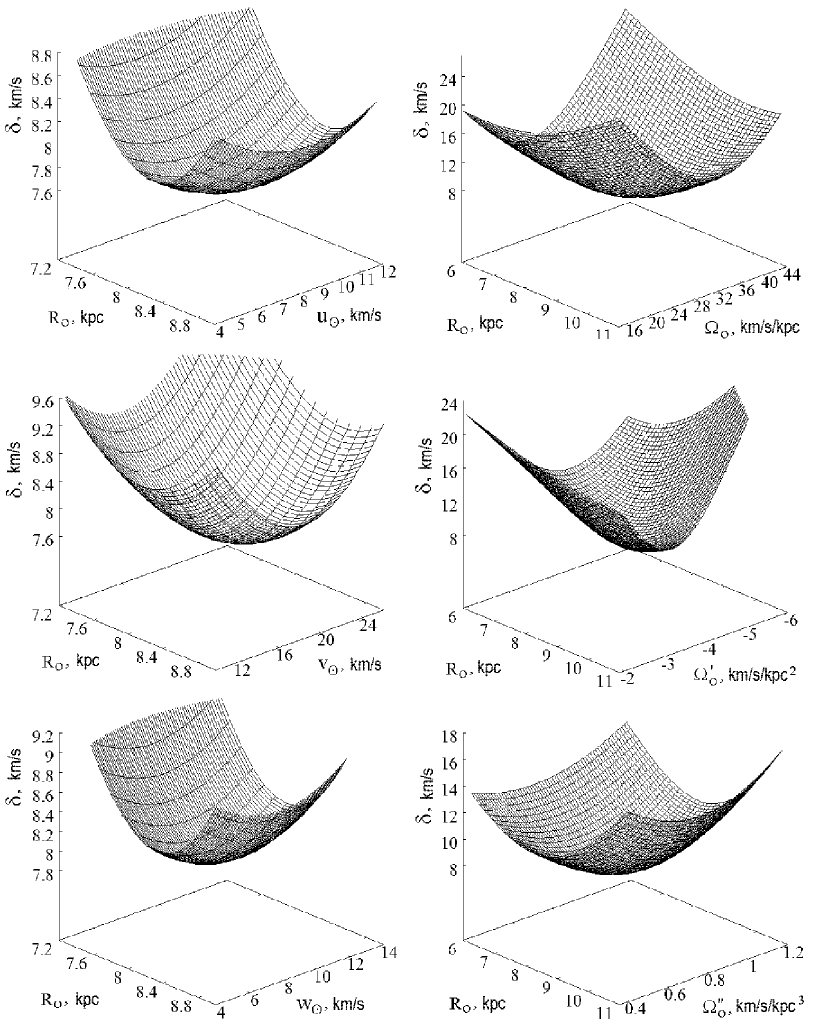
Рис. 1: Graphical representation of the two-dimensional residuals $\delta=\sqrt{F}$ corresponding to solution (9); one of the measurements is specified by the parameter $R_{0}$; one of the parameters $u_{\odot},v_{\odot},w_{\odot},\Omega_{0},\Omega^{\prime}_{0},$ and $\Omega^{\prime\prime}_{0}$ acts as the second measurement; the remaining parameters are fixed at the level of the solutions obtained.

RESULTS

Several approaches to solving the optimization problem (1) with constraints (2)–(4) are known. Since the contribution of Eq. (4) to the general solution is negligible when using distant stars, only Eqs. (2) and (3) may be used. In this case, however, the velocity $w_{\odot}$ is determined poorly; it should be fixed. This method was applied, for example, by Mishurov and Zenina (1999) and Mel’nik et al. (2001).

The local expansion/contraction parameter of the stellar system K is of great importance in analyzing nearby stars associated with the Gould Belt (Bobylev and Bajkova 2013a), where its manifests itself as a positive (expansion) kinematic $K$-effect for young stars within 0.6 kpc of the Sun. A small negative $K$-effect (contraction) manifests itself in the kinematics of various samples of stars within up to 2 kpc of the Sun (Torra et al. 2000; Rybka 2004; Bobylev et al. 2009). No evidence for significant general expansion/contraction of the entire Galaxy has been revealed, except for the region close to the Galactic center where an expanding 3-kpc spiral arm is located (Burton 1988; Dame and Thaddeus 2008; Sanna et al. 2009). Therefore, including the parameter $K$ as an unknown one when analyzing masers is of considerable interest.

Table 2 gives the kinematic parameters found by using the three-dimensional $(V_{r},V_{l},V_{b})$ velocity field of 73 masers. Table 3 gives the kinematic parameters found by using the two-dimensional $(V_{r},V_{l})$ velocity field of the same masers. The solutions obtained both with unit weights and with weights (6) are presented in the tables. The solutions obtained at a fixed solar velocity, $w_{\odot}=7$ km s^-1, are given in the last two columns of the tables. Analysis of the parameters presented in Tables 2 and 3 allows a number of conclusions to be reached. Since the local expansion/contraction parameter of the stellar system $K$ does not differ significantly from zero in all eight solutions, the number of unknown parameters can be reduced. Obviously, the peculiar solar velocity $w_{\odot}$ should be fixed when analyzing the two-dimensional velocity field. However, this quantity is determined with confidence in the case of a three-dimensional analysis. This is because the sample of masers contains a sufficient number of nearby sources. Using the system of weights (6) slightly improves the accuracy of the parameters being determined compared to unit weights. $R_{0}$ is determined with confidence in all eight cases.

We obtained a solution using the three-dimensional maser velocity field with seven unknowns, without the parameter $K,$ and with unit weights:

$$\begin{array}[]{lll}u_{\odot}=6.72\pm 1.02\leavevmode\nobreak\ \hbox{km s${}^{-1}$},\\ v_{\odot}=17.68\pm 0.65\leavevmode\nobreak\ \hbox{km s${}^{-1}$},\\ w_{\odot}=7.89\pm 0.35\leavevmode\nobreak\ \hbox{km s${}^{-1}$},\\ \Omega_{0}=27.81\pm 0.79\leavevmode\nobreak\ \hbox{km s${}^{-1}$ kpc${}^{-1}$},\\ \Omega^{\prime}_{0}=-3.78\pm 0.19\leavevmode\nobreak\ \hbox{km s${}^{-1}$ kpc${}^{-2}$},\\ \Omega^{\prime\prime}_{0}=0.756\pm 0.050\leavevmode\nobreak\ \hbox{km s${}^{-1}$ kpc${}^{-3}$},\\ R_{0}=8.35\pm 0.30\leavevmode\nobreak\ \hbox{kpc}\end{array}$$ (8)

with the error per unit weight $\sigma_{0}=8.10$ km s^-1.

Next, we obtained a similar solution but with weights (6). It has the smallest error per unit weight $\sigma_{0}=7.47$ km s^-1 compared to the results presented in Table 2:

$$\begin{array}[]{lll}u_{\odot}=7.81\pm 0.63\leavevmode\nobreak\ \hbox{km s${}^{-1}$},\\ v_{\odot}=17.47\pm 0.33\leavevmode\nobreak\ \hbox{km s${}^{-1}$},\\ w_{\odot}=7.73\pm 0.23\leavevmode\nobreak\ \hbox{km s${}^{-1}$},\\ \Omega_{0}=28.86\pm 0.45\leavevmode\nobreak\ \hbox{km s${}^{-1}$ kpc${}^{-1}$},\\ \Omega^{\prime}_{0}=-3.96\pm 0.09\leavevmode\nobreak\ \hbox{km s${}^{-1}$ kpc${}^{-2}$},\\ \Omega^{\prime\prime}_{0}=0.790\pm 0.027\leavevmode\nobreak\ \hbox{km s${}^{-1}$ kpc${}^{-3}$},\\ R_{0}=8.33\pm 0.20\leavevmode\nobreak\ \hbox{kpc}.\end{array}$$ (9)

In this case, the linear rotation velocity at the solar distance $R_{0}$ is $V_{0}=241\pm 7$ km s^-1 and the Oort constants $A=0.5R_{0}\Omega_{0}^{\prime}$ and $B=\Omega_{0}+0.5R_{0}\Omega_{0}^{\prime}$ are $A=-16.49\pm 0.60$ km s^-1 kpc^-1 and $B=12.37\pm 1.12$ km s^-1 kpc^-1.

As a clear illustration of the uniqueness of the solution obtained (i.e., the existence of a global minimum of the functional F in a wide range of sought for parameters), Fig. 1 presents the two-dimensional dependences of the residuals $\delta=\sqrt{F}$ (see (1)) on $R_{0}$ and one of the parameters $u_{\odot},v_{\odot},w_{\odot},\Omega_{0},\Omega^{\prime}_{0},$ and $\Omega^{\prime\prime}_{0}$, provided that the remaining parameters are fixed at the level of solutions (9).

Figure 2 presents the Galactic rotation curve constructed with parameters (9) using the value of $R_{0}=8.3$ kpc found; when calculating the boundaries of the confidence region, we took into account the uncertainty in estimating $R_{0}$ of 0.2 kpc.

Таблица 2: Kinematic parameters found by using the three-dimensional ($V_{r},V_{l},V_{b}$) velocity field of 73 masers

Parameters	$w_{r,l,b}=1$	$w_{r,l,b}\neq 1$	$w_{r,l,b}=1$	$w_{r,l,b}\neq 1$
$u_{\odot},$ km s-1	$6.82\pm 0.99$	$7.85\pm 0.55$	$6.80\pm 1.03$	$7.81\pm 0.52$
$v_{\odot},$ km s-1	$17.51\pm 0.61$	$17.32\pm 0.43$	$17.56\pm 0.62$	$17.33\pm 0.42$
$w_{\odot},$ km s-1	$7.90\pm 0.32$	$7.68\pm 0.23$	—	—
$\Omega_{0},$ km s-1 kpc-1	$28.00\pm 0.85$	$28.85\pm 0.50$	$28.02\pm 0.83$	$28.83\pm 0.41$
$\Omega^{{}^{\prime}}_{0},$ km s-1 kpc-2	$-3.86\pm 0.26$	$-3.91\pm 0.10$	$-3.86\pm 0.27$	$-3.90\pm 0.11$
$\Omega^{{}^{\prime\prime}}_{0},$ km s-1 kpc-3	$0.78\pm 0.07$	$0.77\pm 0.03$	$0.78\pm 0.07$	$0.77\pm 0.03$
$K,$ km s-1 kpc-1	$0.02\pm 0.38$	$-0.24\pm 0.18$	$-0.04\pm 0.44$	$-0.28\pm 0.20$
$R_{0},$ kpc	$8.25\pm 0.41$	$8.42\pm 0.16$	$8.25\pm 0.43$	$8.46\pm 0.19$
$\sigma_{0},$ km s-1	8.09	7.74	8.11	7.75

Таблица 3: Kinematic parameters found by using the two-dimensional ($V_{r},V_{l},V_{b}$) velocity field of 73 masers

Parameters	$w_{r,l,b}=1$	$w_{r,l,b}\neq 1$	$w_{r,l,b}=1$	$w_{r,l,b}\neq 1$
$u_{\odot},$ km s-1	$4.47\pm 1.27$	$5.10\pm 0.63$	$6.53\pm 1.15$	$7.45\pm 0.49$
$v_{\odot},$ km s-1	$17.37\pm 0.58$	$17.37\pm 0.36$	$17.44\pm 0.53$	$17.31\pm 0.41$
$w_{\odot},$ km s-1	$36.78\pm 4.86$	$34.91\pm 3.38$	—	—
$\Omega_{0},$ km s-1 kpc-1	$27.45\pm 0.85$	$27.90\pm 0.42$	$27.91\pm 0.96$	$28.71\pm 0.45$
$\Omega^{{}^{\prime}}_{0},$ km s-1 kpc-2	$-3.74\pm 0.22$	$-3.80\pm 0.10$	$-3.81\pm 0.28$	$-3.89\pm 0.11$
$\Omega^{{}^{\prime\prime}}_{0},$ km s-1 kpc-3	$0.75\pm 0.06$	$0.76\pm 0.03$	$0.76\pm 0.07$	$0.77\pm 0.03$
$K,$ km s-1 kpc-1	$-0.17\pm 0.38$	$-0.31\pm 0.18$	$-0.13\pm 0.41$	$-0.29\pm 0.20$
$R_{0},$ kpc	$8.35\pm 0.38$	$8.41\pm 0.18$	$8.37\pm 0.45$	$8.44\pm 0.20$
$\sigma_{0},$ km s-1	8.07	7.30	8.45	7.70

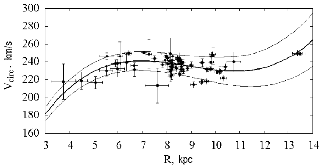
Рис. 2: Galactic rotation curve constructed with parameters (9) (thick line); the thin lines mark the 1у confidence region; the vertical straight line marks the Sun’s position.

Allowance for the Statistical Properties of the Sample of Masers

Although the sample of masers with measured trigonometric parallaxes is small, we can set the objective to refine the parameters $S_{0},$ $\beta$ and $\gamma,$ needed for the calculation of weights (6).

For this purpose, we used the well-known relations between the dispersions $\sigma_{U},\sigma_{V},$ and $\sigma_{W}$ of the velocities $U,V,$ and $W,$ respectively, directed along the heliocentric rectangular coordinate axes and the dispersions $\sigma_{V_{r}},\sigma_{V_{l}},$ and $\sigma_{V_{b}}$ of the velocities $V_{r},V_{l},$ and $V_{b},$ respectively, directed along the observed axes (Crézé and Mennessier 1973):

$$\begin{array}[]{lll}\sigma^{2}_{V_{r}}=\sigma^{2}_{U}\cos^{2}l\cos^{2}b+\sigma^{2}_{V}\sin^{2}l\cos^{2}b+\\ \qquad\sigma^{2}_{W}\sin^{2}b+\varepsilon^{2}_{V_{r}},\\ \sigma^{2}_{V_{l}}=\sigma^{2}_{U}\sin^{2}l+\sigma^{2}_{V}\cos^{2}l+(4.74r)^{2}\varepsilon^{2}_{\mu_{l}},\\ \sigma^{2}_{V_{b}}=\sigma^{2}_{U}\cos^{2}l\sin^{2}b+\sigma^{2}_{V}\sin^{2}l\sin^{2}b+\\ \qquad\sigma^{2}_{W}\cos^{2}b+(4.74r)^{2}\varepsilon^{2}_{\mu_{b}},\end{array}$$ (10)

where $\varepsilon_{V_{r}},\varepsilon_{\mu_{l}},\varepsilon_{\mu_{b}}$ are the observational errors of the corresponding components.

Note that the velocities $U,$ $V,$ and $W$ from which the dispersions are calculated must be the residual ones, i.e., freed from the differential Galactic rotation and the perturbations caused by the influence of the spiral density wave. The available sample of masers is so far insufficient for the necessity of allowance for both effects to be shown in practice. However, previously (Bobylev and Bajkova 2013a), using a sample of 162 nearby O–B2.5 stars as an example, we showed (see Fig. 8 in the cited paper) that allowance for the influence of the spiral density wave reduces tangibly the residual velocity dispersions. In our case, to take into account the influence of the differential Galactic rotation, we used the parameters from solution (9). The spiral density wave parameters were taken from Bobylev and Bajkova (2013b), where they were also determined from masers.

To analyze the residual velocities, we produced a sample of 55 masers satisfying the conditions $\sigma_{\pi}/\pi<10\%$ and $r<3.5$ kpc, i.e., we selected sufficiently distant sources with the most reliably measured distances. After allowance for the differential Galactic rotation and the velocities of the perturbations caused by the influence of the spiral density wave, we obtained the following residual velocity dispersions: $\sigma_{U}=8.2$ km s^-1, $\sigma_{V}=7.1$ km s^-1 and $\sigma_{W}=7.3$ km s^-1. Next, after the substitution of these values into the right parts of Eqs. (10), we found the dispersions ${\overline{\sigma}_{V_{r}}}$, ${\overline{\sigma}_{V_{l}}}$ and ${\overline{\sigma}_{V_{b}}}$ for each object. The dispersions averaged over all objects are $\sigma_{V_{r}}=1.19$ km s^-1, $\sigma_{V_{l}}=1.22$ km s^-1 and $\sigma_{V_{b}}=0.99$ km s^-1, from which we calculated the sought-for coefficients: $\beta=\sigma_{V_{r}}/\sigma_{V_{l}}=0.98$ and $\gamma=\sigma_{V_{r}}/\sigma_{V_{b}}=1.20$. As we see, the derived values of $\beta$ and $\gamma$ are close to unity. The solution of the kinematic equations (2)–(4) for 73 masers using the derived parameters is virtually indistinguishable from solution (9) obtained at $\beta=1$ and $\gamma=1.$

We also considered the case where a coefficient $\gamma$ differing significantly from unity is expected to be obtained. For this purpose, we produced a sample of 24 nearer masers satisfying the conditions $\sigma_{\pi}/\pi<10\%$ and $r<1.5$ kpc. After allowance for the differential Galactic rotation and the velocities of the perturbations caused by the influence of the spiral density wave, we obtained the following residual velocity dispersions: $\sigma_{U}=6.2$ km s^-1, $\sigma_{V}=4.8$ km s^-1 and $\sigma_{W}=3.6$ km s^-1, from which we estimated $S_{0}=\sqrt{\sigma^{2}_{U}+\sigma^{2}_{V}+\sigma^{2}_{W}}=8.6$ km s^-1. Using Eqs. (10) and the subsequent averaging of the individual dispersions, we found $\sigma_{V_{r}}=0.95$ km s^-1, $\sigma_{V_{l}}=0.99$ km s^-1 and $\sigma_{V_{b}}=0.49$ km s^-1, whence $\beta=\sigma_{V_{r}}/\sigma_{V_{l}}=0.96$ and $\gamma=\sigma_{V_{r}}/\sigma_{V_{b}}=1.94$. The new solution of the kinematic equations (2)–(4) for 73 masers with weights (6) and the refined $S_{0}=8.6$ км/с, $\beta=0.96,$ and $\gamma=1.94$ is

$$\begin{array}[]{lll}u_{\odot}=8.58\pm 0.54\leavevmode\nobreak\ \hbox{km s${}^{-1}$},\\ v_{\odot}=17.72\pm 0.42\leavevmode\nobreak\ \hbox{km s${}^{-1}$},\\ w_{\odot}=7.42\pm 0.23\leavevmode\nobreak\ \hbox{km s${}^{-1}$},\\ \Omega_{0}=29.05\pm 0.46\leavevmode\nobreak\ \hbox{km s${}^{-1}$ kpc${}^{-1}$},\\ \Omega^{\prime}_{0}=-3.97\pm 0.09\leavevmode\nobreak\ \hbox{km s${}^{-1}$ kpc${}^{-2}$},\\ \Omega^{\prime\prime}_{0}=0.790\pm 0.028\leavevmode\nobreak\ \hbox{km s${}^{-1}$ kpc${}^{-3}$},\\ R_{0}=8.34\pm 0.16\leavevmode\nobreak\ \hbox{kpc}.\end{array}$$ (11)

In this case, the error per unit weight is $\sigma_{0}=7.53$ km s^-1. It can be seen that the differences between solutions (9) and (11) do not exceed the $1\sigma$ error level. Thus, we obtained close solutions, despite the fact that the weights of the velocities $V_{b}$ (Eq. (4)) increased considerably.

Since the coefficients $\beta\approx 1$ and $\gamma\approx 1$ found above reflect the statistical properties of the original sample of 73 masers more adequately, we consider solution (9) as the basic one. In this case, as our additional simulations showed, a low sensitivity of the solution to changes in the coefficients $\beta$ and $\gamma$ should be noted.

DISCUSSION

The parameters of the Galactic rotation curve we found (see solutions (9) and (11)) are in good agreement with the results of analyzing such young Galactic disk objects as OB associations, $\Omega_{0}=31\pm 1$ km s^-1 kpc^-1 (Mel’nik et al. 2001; Mel’nik and Dambis 2009), blue supergiants, $\Omega_{0}=29.6\pm 1.6$ km s^-1 kpc^-1 and $\Omega^{\prime}_{0}=-4.76\pm 0.32$ km s^-1 kpc^-2 (Zabolotskikh et al. 2002), or distant OB3 stars ($R_{0}=8$ kpc), $\Omega_{0}=31.9\pm 1.1$ km s^-1 kpc^-1, $\Omega^{{}^{\prime}}_{0}=-4.30\pm 0.16$ km s^-1 kpc^-2 and $\Omega^{{}^{\prime\prime}}_{0}=1.05\pm 0.35$ km s^-1 kpc^-3 (Bobylev and Bajkova 2013a). The value of $V_{0}=241\pm 7$ km s^-1 obtained at $R_{0}=8.3$ kpc is in good agreement with $V_{0}=254\pm 16$ km s^-1 at $R_{0}=8.4$ kpc (Reid et al. 2009a) and $V_{0}=244\pm 13$ km s^-1 for $R_{0}=8.2$ kpc (Bovy et al. 2009) determined from a sample of 18 masers. Note also the paper by Irrgang et al. (2013), who proposed three Galactic potential models constructed using data on hydrogen clouds and masers, with the velocity $V_{0}$ having been found to be close to 240 km s^-1 and $R_{0}\approx 8.3$ kpc.

Individual independent methods give an estimate of $R_{0}$ with an error of 10–15%. Note several important isolated measurements. Based on Cepheids and RR Lyr stars belonging to the bulge (collected by Groenewegen et al. 2008) and using improved calibrations derived from Hipparcos data and 2MASS photometry, Feast et al. (2008) obtained an estimate of $R_{0}=7.64\pm 0.21$ kpc. Having analyzed the orbits of stars moving around a massive black hole at the Galactic center (the method of dynamical parallaxes), Gillessen et al. (2009) obtained an estimate of $R_{0}=8.33\pm 0.35$ kpc. According to VLBI measurements, the radio source Sqr A* has a proper motion relative to extragalactic sources of $6.379\pm 0.026$ mas yr^-1 (Reid and Brunthaler 2004); using this value, Schönrich (2012) found $R_{0}=8.27\pm 0.29$ kpc and $V_{0}=238\pm 9$ km s^-1. Two H₂O maser sources, Sgr B2N and Sgr B2M, are in the immediate vicinity of the Galactic center, where the radio source Sqr A* is located. Based on their direct trigonometric VLBI measurements, Reid et al. (2009b) obtained an estimate of $R_{0}=7.9^{+0.8}_{-0.7}$ kpc.

Thus, our kinematic estimate of $R_{0}=8.3\pm 0.2$ kpc is in good agreement with the known estimates and surpasses some of them in accuracy.

CONCLUSIONS

Based on published data, we produced a sample of 73 masers with known line-of-sight velocities and highly accurate trigonometric parallaxes and proper motions measured by VLBI. This allowed the maser velocity field needed to solve Bottlinger’s kinematic equations to be formed. Bottlinger’s kinematic equations we considered relate the Galactic rotation parameters ($\Omega_{0}$ and its derivatives), the solar Galactocentric distance $(R_{0}),$ the object group velocity components relative to the Sun ($u_{\odot},v_{\odot},w_{\odot}$), and the system expansion/contraction parameter (the $K$ effect). The method of minimizing the quadratic functional that is the sum of the weighted squares of the residuals of measurements and model velocities was used to find the unknown parameters. Solutions were found in the cases of both three-dimensional and two-dimensional velocity fields for various numbers of sought-for parameters when various weighting methods were applied. In all cases, the $K$ effect turned out to be statistically insignificant. We established that the solution obtained from the three-dimensional maser velocity field for seven sought-for parameters ($u_{\odot},v_{\odot},w_{\odot},\Omega_{0},\Omega^{\prime}_{0},\Omega^{\prime\prime}_{0},$ and $R_{0}$) corresponding to the global minimum of the functional in a wide range of their variations is most reliable. This solution is (9). The linear rotation velocity at the solar distance $R_{0}$ is $V_{0}=241\pm 7$ km s^-1. The solar Galactocentric distance $R_{0}$ is the most important and debatable parameter. Our value is in good agreement with the most recent estimates and even surpasses them in accuracy.

REFERENCES

1. A.T. Bajkova and V.V. Bobylev, Astron. Lett. 38, 549 (2012).

2. V.V. Bobylev, A.T. Bajkova, and S.V. Lebedeva, Astron. Lett. 33, 720 (2007).

3. V.V. Bobylev, A.T. Bajkova, and A.S. Stepanishchev, Astron. Lett. 34, 515 (2008).

4. V.V. Bobylev, A.S. Stepanishchev, A.T. Bajkova, and G.A. Gontcharov, Astron. Lett. 35, 836 (2009).

5. V.V. Bobylev and A.T. Bajkova, Mon. Not. R. Astron. Soc. 408, 1788 (2010).

6. V.V. Bobylev and A.T. Bajkova, Astron. Lett. 39, 532 (2013a).

7. V.V. Bobylev and A.T. Bajkova, Astron. Lett. 39, 809 (2013b).

8. J. Bovy, D.W. Hogg, and H.-W. Rix, Astrophys. J. 704, 1704 (2009).

9. A. Brunthaler, M.J. Reid, K.M. Menten, et al., Astron. Nachr. 332, 461 (2011).

10. W.B. Burton, Galactic and Extragalactic Radio Astronomy, Ed. by G. Verschuur and K. Kellerman (Springer, New York, 1988).

11. D.P. Clemens, Astrophys. J. 295, 422 (1985).

12. M. Creźeánd M O. Mennessier, Astron. Astrophys. 27, 281 (1973).

13. T.M. Dame and P. Thaddeus, Astron. Astrophys. 683, 143 (2008).

14. S. Dzib, L. Loinard, L.F. Rodriguez, et al., Astrophys. J. 733, 71 (2011).

15. M.W. Feast, C.D. Laney, T.D. Kinman, et al., Mon. Not. R. Astron. Soc. 386, 2115 (2008).

16. T. Foster and B. Cooper, ASP Conf. Ser. 438, 16 (2010).

17. C. Francis and E. Anderson, arXiv:1309.2629 (2013).

18. S. Gillessen, F. Eisenhauer, S. Trippe, et al., Astrophys. J. 692, 1075 (2009).

19. M.A.T. Groenewegen, A. Udalski, and G. Bono, Astron. Astrophys. 481, 441 (2008).

20. T. Hirota, T. Bushimata, Y.K. Choi, et al., Publ. Astron. Soc. Jpn. 59, 897 (2007).

21. A. Irrgang, B. Wilcox, E. Tucker, and L. Schiefelbein, Astron. Astrophys. 549, 137 (2013).

22. M.K. Kim, T. Hirota, M. Honma, et al., Publ. Astron. Soc. Jpn. 60, 991 (2008).

23. E.S. Levine, C. Heiles, and L. Blitz, Astrophys. J. 679, 1288 (2008).

24. Z.M. Malkin, Astron. Rep. 57, 128 (2013).

25. N.M. McClure-Griffiths and J.M. Dickey, Astrophys. J. 671, 427 (2007).

26. P.J. McMillan and J.J. Binney, Mon. Not. R. Astron. Soc. 402, 934 (2010).

27. A.M. Mel’nik, A.K. Dambis, and A S. Rastorguev, Astron. Lett. 27, 521 (2001).

28. A.M. Mel’nik and A.K. Dambis, Mon. Not. R. Astron. Soc. 400, 518 (2009).

29. Yu. N. Mishurov and I.A. Zenina, Astron. Astrophys. 341, 81 (1999).

30. T. Nagayama, T. Omodaka, T. Handa, et al., Publ. Astron. Soc. Jpn. 63, 719 (2011).

31. I.I. Nikiforov, ASP Conf. Ser. 316, 199 (2004).

32. A.S. Rastorguev, E.V. Glushkova, A.K. Dambis, and M.V. Zabolotskikh, Astron. Lett. 25, 595 (1999).

33. M.J. Reid, Ann. Rev. Astron. Astrophys. 31, 345 (1993).

34. M.J. Reid and A. Brunthaler, Astrophys. J. 616, 872 (2004).

35. M.J. Reid, K.M. Menten, X.W. Zheng, et al., Astrophys. J. 700, 137 (2009a).

36. M. Reid, K.M. Menten, X.W. Zheng, et al., Astrophys. J. 705, 1548 (2009b).

37. S.P. Rybka, Kinem. Fiz. Nebesn. Tel 20, 133 (2004).

38. K.L.J. Rygl, A. Brunthaler, M.J. Reid, et al., Astron. Astrophys. 511, A2 (2010).

39. A. Sanna, M.J. Reid, L. Moscadelli, et al., Astrophys. J. 706, 464 (2009).

40. R. Schönrich, Mon. Not. R. Astron. Soc. 427, 274 (2012).

41. J. Torra, D. Fernández, and F. Figueras, Astron. Astrophys. 359, 82 (2000).

42. R.M. Torres, L. Loinard, A.J. Mioduszewski, et al., Astrophys. J. 698, 242 (2009).

43. Y. Xu, J.J. Li, M.J. Reid, et al., Astrophys. J. 769, 15 (2013).

44. M.V. Zabolotskikh, A.S. Rastorguev, and A.K. Dambis, Astron. Lett. 28, 454 (2002).

45. B. Zhang, M.J. Reid, K.M. Menten, et al., Astrophys. J. 775, 79 (2013).