Ensemble Simulations of Proton Heating in the Solar Wind via Turbulence and Ion Cyclotron Resonance

Abstract

Protons in the solar corona and heliosphere exhibit anisotropic velocity distributions, violation of magnetic moment conservation, and a general lack of thermal equilibrium with the other particle species. There is no agreement about the identity of the physical processes that energize non-Maxwellian protons in the solar wind, but a traditional favorite has been the dissipation of ion cyclotron resonant Alfvén waves. This paper presents kinetic models of how ion cyclotron waves heat protons on their journey from the corona to interplanetary space. It also derives a wide range of new solutions for the relevant dispersion relations, marginal stability boundaries, and nonresonant velocity-space diffusion rates. A phenomenological model containing both cyclotron damping and turbulent cascade is constructed to explain the suppression of proton heating at low alpha–proton differential flow speeds. These effects are implemented in a large-scale model of proton thermal evolution from the corona to 1 AU. A Monte Carlo ensemble of realistic wind speeds, densities, magnetic field strengths, and heating rates produces a filled region of parameter space (in a plane described by the parallel plasma beta and the proton temperature anisotropy ratio) similar to what is measured. The high-beta edges of this filled region are governed by plasma instabilities and strong heating rates. The low-beta edges correspond to weaker proton heating and a range of relative contributions from cyclotron resonance. On balance, the models are consistent with other studies that find only a small fraction of the turbulent power spectrum needs to consist of ion cyclotron waves.

1. Introduction

The Sun’s high-temperature corona expands into the heliosphere as a supersonic, magnetized, and weakly collisional solar wind. Despite many years of study, there is still no comprehensive understanding of the physical processes that generate this highly energized state. Furthermore, it is unclear to what extent the solar wind detected in interplanetary space preserves sufficient information from the corona to help us learn how the plasma was heated initially. It has been known for several decades that elemental abundances and ionization fractions measured at 1 AU must be “frozen in” at low heights in the solar atmosphere (e.g., Zurbuchen, 2007). However, the temperatures and detailed velocity distribution functions (VDFs) of ions and electrons appear to evolve gradually through the heliosphere (Matteini et al., 2012) and in some cases they may be affected by instabilities that become activated near the detecting spacecraft (Gary et al., 2001).

What are the processes that affect the thermodynamics of positive ions as they accelerate away from the solar corona? Because of infrequent Coulomb collisions above the coronal base, particles that flow along magnetic field lines should want to conserve their magnetic moments (Chew et al., 1956). Hartle & Sturrock (1968) found that without any other source of heating, magnetic moment conservation would produce extremely cold and beamed (in the parallel sense; $T_{\parallel}\gg T_{\perp}$) heliospheric protons, which is not seen (e.g., Marsch, 2012). In fact, at 1 AU the majority of proton VDFs are close to isotropic, which seems to require some residual or anomalous coupling via collisions (Griffel & Davis, 1969; Livi & Marsch, 1987). Heat conduction is an important carrier of thermal energy for electrons, but not so much for protons (Sandbaek & Leer, 1995). The dominant sources of thermal energy for protons are believed to be the irreversible decays of plasma structures; i.e., dissipation of waves, shredding of turbulent eddies, and multiple types of energy conversion in current sheets associated with magnetic reconnection.

The goal of this paper is to determine the consequences of one specific proposed idea for proton heating in the solar wind: the dissipation of ion cyclotron resonant waves. Although other sources of heat are likely to exist, we find it useful to explore how much can be explained by restricting ourselves to just a single main process. This mechanism has been studied extensively (see reviews by Hollweg & Isenberg, 2002; Marsch, 2006), but often the microphysics of wave-particle interactions are decoupled from the macrophysics of VDF transport from the corona to 1 AU. Thus, this paper aims to provide an in-depth study of how the microphysics and macrophysics depend on one another. Several well-known pieces of the puzzle will be assembled together in new ways.

Section 2 summarizes the wide range of suggested physical explanations for ion heating in the solar wind and lays out many of the open questions. Section 3 begins our focused look at the ion cyclotron resonance mechanism by deriving several versions of the wave dispersion relation. Section 4 discusses the net transfer of energy from the waves to the anisotropic particle VDFs. Section 5 presents a model of how drifting alpha particles may suppress the cyclotron heating available to heliospheric protons. Section 6 assembles the above results into a large-scale model of radial energy transport from the corona to 1 AU, and it shows how the observed distribution of states (in a plane described by the parallel plasma beta and temperature anisotropy ratios of protons) is explainable as a consequence of ion cyclotron heating. Section 7 concludes with a discussion of some of the wider implications of this work and gives suggestions for future improvements.

2. A Walk Through the Ion Heating Maze

Prior to delving into the primary physical process studied in this paper, it is useful to list the alternatives. Ideally, each of the proposed heating mechanisms should be tested in a similar way as the ion cyclotron resonance idea is put through its paces in Sections 3–6 below. Here we are able to discuss only a fraction of the large number of papers that presented ideas for the kinetic energization of ions in the solar wind; for other reviews, see Hollweg (2008), Cranmer (2009), and Ofman (2010). Also, since our goal is to study collisionless processes that give rise to preferential ion heating and acceleration, we neglect the much broader literature of strictly magnetohydrodynamic (MHD) theories that do not focus on the kinetic consequences of coronal heating (see, e.g., Klimchuk, 2006; Parnell & De Moortel, 2012).

Particle and field instruments at heliocentric distances greater than 0.3 AU have detected several marked departures from thermal equilibrium for protons and other ions (Neugebauer, 1982; Marsch, 2006; Kasper et al., 2008). In the fast solar wind, ions tend to be heated more strongly than electrons, and protons often exhibit VDF anisotropies with temperatures measured in the direction perpendicular to the magnetic field often exceeding temperatures parallel to the field (i.e., $T_{\perp}>T_{\parallel}$). Marsch et al. (1983) found that proton magnetic moments are not conserved between 0.3 and 1 AU in the fast wind; they increase steadily, implying a gradual input of perpendicular kinetic energy. Also, most heavy ion species flow faster than the protons by about the local Alfvén speed (Hefti et al., 1998; Berger et al., 2011). These measurements were augmented by spectroscopic observations of similar extreme properties in low-density coronal holes (Kohl et al., 1997, 2006; Wilhelm et al., 2011).

Many of the models proposed to explain the proton and ion measurements involve the damping of MHD waves. However, there is little agreement about the most relevant wave types, the dominant wave generation mechanisms, or the precise means of dissipation. Quite a few of the models also involve a broad array of multiple steps of energy conversion between waves, turbulent eddies, reconnection structures, and other nonlinear plasma features. Nevertheless, it was noticed early on (Abraham-Shrauner & Feldman, 1977; Hollweg & Turner, 1978) that one specific mechanism—cyclotron resonance between left-hand polarized Alfvén waves and ion Larmor orbits—appears to naturally produce many of the observed particle properties (see, e.g., Marsch, 2006; Hollweg, 2008). Resonant ions “surf” along with a wave’s oscillating electric and magnetic fields, and they experience secular gains or losses in energy depending on phase. For a random distribution of wave phases, ions undergo a diffusive random walk in velocity space (Kennel & Engelmann, 1966; Rowlands et al., 1966).

One major problem with the ion cyclotron model is that the resonant wave frequencies $f$ in the corona are of order $10^{2}$ to $10^{4}$ Hz. These frequencies are substantially higher than those inferred for observed Alfvén waves (e.g., $f\lesssim 0.01$ Hz; see Jess et al., 2009; McIntosh et al., 2011), and it is difficult find a process that bridges that gap. Axford & McKenzie (1992) and Tu & Marsch (1997) proposed that the low solar atmosphere produces a continuous frequency spectrum of MHD waves that extends up to $\sim$10⁴ Hz. As the waves propagate up into the corona, the high-frequency end of the spectrum becomes eroded as the local Larmor frequency decreases with increasing height. However, Cranmer (2000, 2001) argued that heavy ions with low gyrofrequencies would likely be able to intercept nearly all of the available wave energy prior to it becoming resonant with protons and alpha particles. Also, Hollweg (2000) found that the radio scintillation signature of a basal spectrum of ion cyclotron waves would appear quite different from what is already observed in the corona. Thus, the idea that ion cyclotron waves are copiously generated at the solar surface has fallen slightly out of favor, and other explanations have been pursued.

A potentially more robust way to generate small-scale (i.e., high-frequency) plasma oscillations is to invoke a nonlinear turbulent cascade. Strong MHD turbulence is certainly present throughout the heliosphere (see reviews by Tu & Marsch, 1995; Matthaeus & Velli, 2011; Bruno & Carbone, 2013). Turbulent dissipation also appears able to provide the right order of magnitude of heat to both the corona and solar wind (e.g., Dmitruk et al., 2002; Cranmer et al., 2007; Perez & Chandran, 2013; Lionello et al., 2014). Many models invoke the idea that solar flux tubes are jostled by photospheric granular motions, and this propels Alfvén waves into the corona that partially reflect back down to produce counterpropagating wave packets. Collisions of these wave packets are believed to drive an efficient nonlinear cascade to small scales (Howes & Nielson, 2013), but the ultimate dissipation mechanisms are usually not identified in these models (see also Bingert & Peter, 2011; Matsumoto & Suzuki, 2014).

A distinguishing feature of MHD turbulence in the presence of a strong background magnetic field is an anisotropic cascade in wavenumber space. Specifically, the breakup of eddies into smaller scales occurs primarily in directions perpendicular to the field (e.g., Strauss, 1976; Montgomery & Turner, 1981; Shebalin et al., 1983; Goldreich & Sridhar, 1995). The basic cascade process is not expected to produce fluctuations with high parallel wavenumbers $k_{\parallel}$, and thus it is not expected to directly excite much wave energy at the ion cyclotron resonance. Spacecraft have detected anisotropic turbulent power spectra in interplanetary space that generally agree with these predictions (Horbury et al., 2008; Chen et al., 2010; Sahraoui et al., 2010), though there is also evidence that a fraction of the fluctuation energy can be in the form of high-frequency waves (see below).

If one treats the small-scale fluctuations in an MHD cascade as linear waves, the dominant low-frequency modes at wavenumbers $k_{\perp}\approx\rho_{p}^{-1}$, where $\rho_{p}$ is the proton thermal gyroradius, are the kinetic Alfvén wave (KAW) and the magnetosonic whistler wave. In collisionless plasmas, these modes tend to dissipate via a combination of Landau and transit-time damping. For conditions appropriate to the corona and heliosphere, the KAW mode seems to be most prevalent (Salem et al., 2012; Podesta, 2013; Chen et al., 2013; Roberts et al., 2013). Although linear KAW damping may one way of producing the fast proton beams seen in interplanetary space (Voitenko & Pierrard, 2013), most of their energy goes into parallel electron heating (Leamon et al., 1999; Cranmer & van Ballegooijen, 2003; Gary & Borovsky, 2008) and not the perpendicular ion heating that is observed.

For the last decade, there has been much work devoted to finding the ways that low-frequency, high-$k_{\perp}$ turbulent fluctuations can heat protons and heavy ions. If KAW amplitudes become sufficiently high, the Larmor orbits of protons and ions become stochastic. This in turn enables low-energy particles to undergo random-walk migration to higher energies, and this effectively produces perpendicular heating (e.g., Johnson & Cheng, 2001; Voitenko & Goossens, 2004; Chandran, 2010; Chandran et al., 2011, 2013; Bourouaine & Chandran, 2013). Alternately, KAW Landau damping may give rise to enough parallel particle acceleration to produce beamed electron VDFs (Haynes et al., 2014) that themselves are unstable to the growth of Langmuir waves and electrostatic “phase space holes.” The latter have been suggested as possible sources of perpendicular scattering for protons and ions (Matthaeus et al., 2003; Cranmer & van Ballegooijen, 2003). Still another idea is that turbulence may produce sufficiently strong plasma inhomogeneities—i.e., velocity shears or cross-field density gradients—that the system may become unstable to the rapid growth of ion cyclotron waves (see Markovskii, 2001; Markovskii et al., 2006; Vranjes & Poedts, 2008; Mikhailenko et al., 2008; Rudakov et al., 2012).

It is possible that the smallest-scale fluctuations in MHD turbulence are not accurately describable by a superposition of linear waves. Many simulations show that plasma turbulence eventually results in the presence of intermittent vortices separated by thin current sheets (e.g., Karimabadi et al., 2013). Both test-particle models (Dmitruk et al., 2004; Parashar et al., 2009; Lehe et al., 2009; Lynn et al., 2012) and full Vlasov kinetic simulations (Servidio et al., 2012, 2014) have shown that positive ions can interact resonantly with turbulent current sheets and become heated perpendicularly. A related idea is that when ions cross from the sub-Alfvénic reconnection inflow to the super-Alfvénic outflow region, they may undergo perpendicular acceleration via a rapid pickup-like process (Drake et al., 2009; Artemyev et al., 2014). There are also some ways that nonlinear Alfvénic fluctuations may drive different modes of ion VDF diffusion than the ones predicted by classical linear or quasilinear wave theory (e.g., Markovskii et al., 2009; Dong & Singh, 2013; Nariyuki et al., 2014).

Despite the well-known tendency for MHD turbulence to be dominated by a perpendicular cascade of low-frequency eddies (see also Matthaeus et al., 1999; Howes et al., 2008), there is some observational evidence for the existence of ion cyclotron waves. There are time periods in which the solar wind exhibits nearly monochromatic bursts of oscillation at or near the local Larmor frequency (Tsurutani et al., 1994; Jian et al., 2009, 2010). Additional empirical correlations between variance anisotropies, the magnetic field geometry, and various helicity indices indicate that a non-negligible fraction of the fluctuation energy can be in the form of high-frequency Alfvén waves (He et al., 2011; Smith et al., 2012). In the fast solar wind at $\sim$0.3 AU, non-Maxwellian shapes of proton VDFs appear to be consistent with the velocity-space diffusion that occurs in ion cyclotron wave dissipation (Marsch & Tu, 2001b; Bourouaine et al., 2011).

In addition to direct and indirect measurements of wave activity at the ion cyclotron resonance, there are also quite a few studies of the low-wavenumber inertial range (e.g., Bieber et al., 1996; Dasso et al., 2005; MacBride et al., 2008) that indicate the presence of power-law spectra that extend to high values of both $k_{\perp}$ and $k_{\parallel}$. Even though the high-$k_{\parallel}$ spectra are not typically seen to extend all the way up to ion cyclotron resonant wavenumbers, they do hint at the existence of a kind of “parallel cascade.” Some models of MHD turbulence predict a weakened parallel cascade that depends on higher-order wave-wave couplings than the basic ones driving the perpendicular cascade (Ng & Bhattacharjee, 1996; Medvedev, 2000; Maron & Goldreich, 2001). Other models propose that nonlinear couplings between Alfvén and fast-mode waves produce a high-$k_{\parallel}$ enhancement in the Alfvénic spectrum because of the nearly isotropic cascade of the fast-mode waves (Chandran, 2005, 2008; Cranmer & van Ballegooijen, 2012).

In this paper we will study the kinetic and thermodynamic consequences of ion cyclotron resonant waves in the solar wind. Chandran et al. (2010) and Isenberg (2012) discussed several reasons why a population of these waves may be dominated by nearly parallel propagation (i.e., $k_{\parallel}\gg k_{\perp}$) if they are present, and we restrict our analysis to this limiting wavenumber condition as well. We do not directly specify the origin of the ion cyclotron waves, but merely note here that several of the mechanisms discussed above—e.g., instabilities, multi-mode coupling, or a true parallel cascade—may generate them gradually. We do not require ion cyclotron waves to be the dominant form of MHD fluctuation in the corona and solar wind, and in fact the results presented below agree with earlier studies (Isenberg & Vasquez, 2011; Cranmer & van Ballegooijen, 2012) that found only a small fraction of the total wave energy needs to be cyclotron resonant. Thus, this work is largely consistent with other models in which the turbulent cascade is dominated by low-frequency KAW-like fluctuations.

3. Parallel Alfvén Wave Dispersion Relations

Several key properties of the combined system of fluctuations and background conditions depend on the dispersion relation of linear MHD waves. This section describes a number of different approaches that have been used to describe the frequency of small-amplitude left-hand polarized waves propagating parallel to a constant magnetic field ${\bf B}_{0}$. In general, the angular frequency $\omega$ is a complex function of the real parallel wavenumber $k_{\parallel}$. For reasons summarized above, we assume a vanishingly small perpendicular wavenumber $k_{\perp}$, which implies that the propagation angle $\theta=\tan^{-1}(k_{\perp}/k_{\parallel})\approx 0$.

For particle VDFs that remain gyrotropically symmetric around the ${\bf B}_{0}$ axis (and thus depend only on velocities $v_{\parallel}$ and $v_{\perp}$ parallel and perpendicular to the field, respectively), the complex dielectric constant $\epsilon$ is given by

$$\epsilon\,=\,1+\sum_{s}\frac{4\pi q_{s}^{2}}{m_{s}\omega^{2}}\int\frac{d^{3}{\bf v}}{\omega-k_{\parallel}v_{\parallel}-\Omega_{s}}\left(\frac{v_{\perp}}{2}\right)\hat{\Sigma}f_{s}({\bf v})$$ (1)

where the sum is taken over each species $s$ of particles having masses $m_{s}$ and charges $q_{s}$ (see, e.g., Montgomery & Tidman, 1964; Stix, 1992). Each species’ VDF is denoted by $f_{s}({\bf v})$ and is normalized to the total number density $n_{s}$ when integrated over all three dimensions of velocity space. In cylindrically symmetric (gyrotropic) coordinates, $d^{3}{\bf v}=2\pi v_{\perp}dv_{\perp}dv_{\parallel}$. Each particle species also has its own Larmor gyrofrequency $\Omega_{s}=q_{s}B_{0}/m_{s}c$, and the pitch-angle derivative operator $\hat{\Sigma}$ is defined as

$$\hat{\Sigma}\,=\,\left(\omega-k_{\parallel}v_{\parallel}\right)\frac{\partial}{\partial v_{\perp}}\,+\,k_{\parallel}v_{\perp}\frac{\partial}{\partial v_{\parallel}}\,\,.$$ (2)

The solution to the dispersion relation is given by finding the appropriate roots of

$$\epsilon\,=\,k_{\parallel}^{2}c^{2}/\omega^{2}\,\,.$$ (3)

In this paper the sum over $s$ is limited to three possible species: electrons ($e$), protons ($p$), and alpha particles ($\alpha$). The electrons are assumed to always follow the Maxwellian cold plasma limit described below, and we assume the wave frequency always obeys $|\omega/\Omega_{e}|\ll 1$.

3.1. Bi-Maxwellian Velocity Distributions

Many general properties of cyclotron resonant waves can be studied in the simple limit of a bi-Maxwellian or two-temperature particle distribution function. For the proton VDF, we can assume

$$f_{p}(v_{\parallel},v_{\perp})=\frac{n_{p}}{\pi^{3/2}w_{p\parallel}w_{p\perp}^{2}}\exp\!\left[-\left(\frac{v_{\parallel}-u_{p\parallel}}{w_{p\parallel}}\right)^{2}-\left(\frac{v_{\perp}}{w_{p\perp}}\right)^{2}\right]$$ (4)

where the proton number density is $n_{p}$ and the thermal spread is described by temperatures parallel and perpendicular to the field ($T_{p\parallel}$ and $T_{p\perp}$ respectively). The corresponding thermal speeds are

$$w_{p\parallel}^{2}=\frac{2k_{\rm B}T_{p\parallel}}{m_{p}}\,\,,\,\,\,\,\,w_{p\perp}^{2}=\frac{2k_{\rm B}T_{p\perp}}{m_{p}}\,\,,$$ (5)

with Boltzmann’s constant given by $k_{\rm B}$ and the anisotropy ratio defined as ${\cal R}_{p}=T_{p\perp}/T_{p\parallel}$. The models below will be applied in the local rest frame of the accelerating solar wind, which for a pure proton–electron plasma implies that $u_{p\parallel}=0$.

Even when using the simplified VDF of Equation (4), there are several levels of approximation that can be applied when solving for the complex wave frequency $\omega=\omega_{r}+i\gamma$. By convention, the linear fluctuations vary as $e^{-i\omega t}$, so $\gamma>0$ corresponds to unstable wave growth. The most general way to solve Equation (3) is to locate all of its roots numerically for each desired wavenumber. These solutions, often called solutions to the Vlasov–Maxwell equations, have been presented extensively in the literature for conditions relevant to the solar wind (e.g., Gary, 1993; Cranmer & van Ballegooijen, 2003, 2012; Gary & Borovsky, 2004; Seough & Yoon, 2009; Yoon et al., 2010; Maruca et al., 2012).

The limiting case of weak instability or decay ($|\gamma/\omega_{r}|\ll 1$) gives rise to some interesting closed-form solutions of the dispersion relation. Following, e.g., Davidson (1983) and Benz (1993), the dielectric constant can be written in this limit as

$$\mbox{Re}(\epsilon)\,=\,1+\sum_{s}\left(\frac{\omega_{ps}}{\omega}\right)^{2}\,\left\{\xi_{0}Z(\xi_{1})+\left({\cal R}_{s}-1\right)\left[1+\xi_{1}Z(\xi_{1})\right]\right\}\,\,,$$ (6)

$$\mbox{Im}(\epsilon)\,=\,\sum_{s}\left(\frac{\omega_{ps}}{\omega}\right)^{2}\,\left\{\pi^{1/2}\exp(-\xi_{1}^{2})\left[{\cal R}_{s}\xi_{1}+\frac{\Omega_{s}}{k_{\parallel}w_{\parallel}}\right]\right\}\,\,,$$ (7)

where the plasma frequencies are defined as $\omega_{ps}^{2}=4\pi q_{s}^{2}n_{s}/m_{s}$. The dimensionless resonance parameter is given by

$$\xi_{n}\,\equiv\,\frac{\omega_{r}-k_{\parallel}u_{s\parallel}-n\Omega_{s}}{k_{\parallel}w_{s\parallel}}$$ (8)

and the parallel drift speed $u_{s\parallel}$ is defined relative to the local bulk (center of mass) speed of the plasma. As above, we assume that $u_{p\parallel}=0$, but the value for alpha particles may be nonzero. The assumption of a Maxwellian VDF shape along any one direction is encapsulated in the dimensionless plasma dispersion function, which is defined as

$$Z(\xi)\,\equiv\,\frac{1}{\sqrt{\pi}}\,{\cal P}\!\int_{-\infty}^{+\infty}\frac{dt\,e^{-t^{2}}}{t-\xi}$$ (9)

where ${\cal P}$ denotes the Cauchy principal value (see Fried & Conte, 1961).

In the small-$\gamma$ limit, the real part of the dispersion relation is simply $\mbox{Re}(\epsilon)=k_{\parallel}^{2}c^{2}/\omega_{r}^{2}$. For convenience, we define dimensionless variables

$$x\,\equiv\,\frac{k_{\parallel}V_{\rm A}}{\Omega_{p}}\,\,,\,\,\,\,\,\,y\,\equiv\,\frac{\omega_{r}}{\Omega_{p}}$$ (10)

where $\omega_{r}$ is the real part of the frequency, and the Alfvén speed is given by

$$V_{\rm A}\,=\,\frac{B_{0}}{\sqrt{4\pi\rho}}\,\,,\,\,\,\,\mbox{with}\,\,\,\rho\,=\,\sum_{s}m_{s}n_{s}\,\,.$$ (11)

All of the solutions below make the nonrelativistic approximation of $V_{\rm A}\ll c$, which is equivalent to ignoring the unity term in Equation (6) and thus neglecting the displacement current in Ampère’s law.

In the limit of small wavenumbers ($|x|\ll 1$), isotropic VDFs (${\cal R}=1$), and a pure proton–electron plasma, the dispersion relation reduces to the ideal MHD expression for Alfvén waves,

$$y\,=\,x\,\,.$$ (12)

If the small-wavenumber approximation is relaxed, the “cold plasma” dispersion relation for cyclotron waves can be derived by taking the large-argument asymptotic limit for the dispersion function,

$$Z(\xi)\,\approx\,-\frac{1}{\xi}\,\,.$$ (13)

Equation (6) is then solved to obtain

$$x^{2}=\frac{y^{2}}{1-y}\,\,,$$ (14)

or

$$y=\frac{x}{2}\left(\sqrt{x^{2}+4}-x\right)$$ (15)

(see, e.g., Cuperman et al., 1975; Dusenbery & Hollweg, 1981; Hollweg & Isenberg, 2002). In this limiting case, the frequency does not depend on either $T_{p\parallel}$ or $T_{p\perp}$.

The cold plasma dispersion relation has been generalized to include the effect of additional ion species that drift relative to the protons. Let us assume a relative alpha particle abundance $h=n_{\alpha}/n_{p}$, and that the ions are flowing ahead of the protons with a known value of $\delta_{\alpha p}=(u_{\alpha\parallel}-u_{p\parallel})/V_{\rm A}$. In the solar wind, $0\leq\delta_{\alpha p}\leq 1$. The ion drift necessitates a more precise accounting of the overall charge neutrality and zero-current conditions in the plasma. Following Gomberoff & Elgueta (1991), Hollweg & Isenberg (2002), and others, the dispersion relation becomes

$$x^{2}=\frac{y^{2}}{1-y}+\frac{4h(y-x\delta_{\alpha p})^{2}}{1-2(y-x\delta_{\alpha p})}\,\,.$$ (16)

In general there are two separate branches of the dispersion relation (e.g., Isenberg, 1984a). Although there has been some work showing that both branches may be excited in some situations (Gomberoff et al., 1994; Tu et al., 2003), for simplicity we assume that only the lowest frequency branch is populated by wave power that cascades from low-wavenumber fluctuations.

Figure 1(a) shows various solutions to the cold plasma dispersion relations. Equation (14) describes the solution without alpha particles, which has the highest frequency in this panel. Figure 1(a) also shows the lower branch for a common solar wind value of $h=0.05$ and a range of drift speeds ($0<\delta_{\alpha p}<0.2$), for which the lowest-$y$ roots of Equation (16) were found numerically. When $\delta_{\alpha p}\gtrsim 0.3$, the alpha particles have essentially drifted out of resonance and the lower dispersion branch is indistinguishable from the case of $h=0$ (see also Hollweg & Isenberg, 2002).

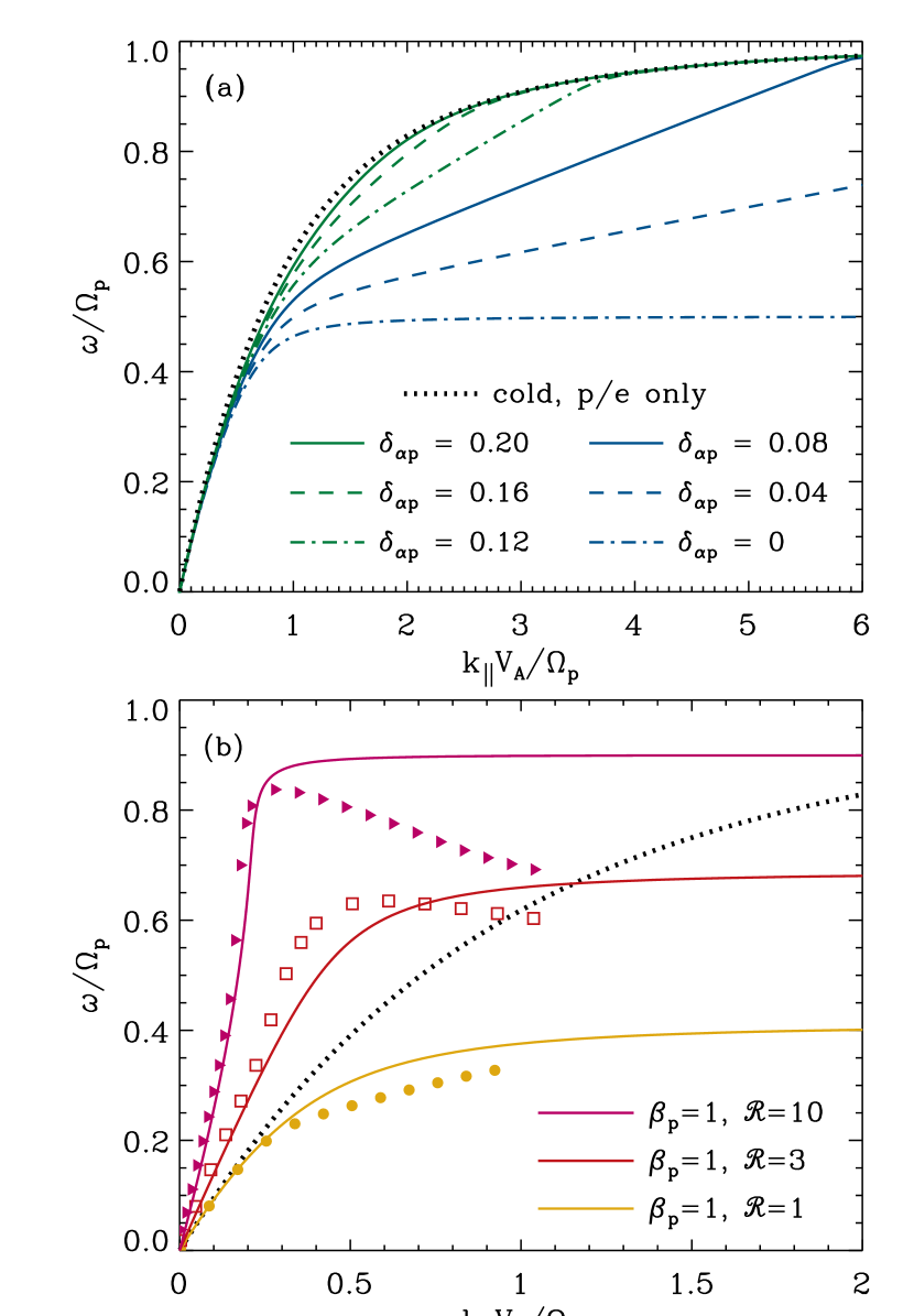
Figure 1.— Dispersion relations for parallel propagating ion cyclotron waves. In both panels, the cold plasma dispersion for a proton–electron plasma is denoted by a black dotted curve. (a) Variation of frequency for cold plasma with 5% alpha particles by number (blue and green curves, labeled by their values of $\delta_{\alpha p}$). (b) Warm plasma dispersion computed using Equation (18) (solid curves) and with numerical Vlasov–Maxwell dispersion code (symbols). These curves were computed with $\beta=1$; see labels for values of the anisotropy ratio ${\cal R}$.

An improved solution to the dispersion relation can be found by beginning to take into account the proton thermal spread. Including the next term in the asymptotic series expansion for $Z(\xi)$ yields such a “warm plasma” dependence on temperature. Thus, the approximation

$$Z(\xi)\,\approx\,-\frac{1}{\xi}-\frac{1}{2\xi^{3}}$$ (17)

is inserted into Equation (6) as before. For a pure proton–electron mixture, the analytic dispersion relation becomes

$$y^{2}=x^{2}(1-y)\left\{1+\frac{\beta}{2(y-1)^{2}}\left[{\cal R}-1+\left(\frac{y}{y-1}\right)\right]\right\}$$ (18)

where for brevity the subscript $p$ has been removed from the anisotropy ratio ${\cal R}$ and the parallel proton plasma beta is defined as

$$\beta\,=\,\frac{w_{p\parallel}^{2}}{V_{\rm A}^{2}}\,=\,\frac{8\pi n_{p}k_{\rm B}T_{p\parallel}}{B_{0}^{2}}\,\,.$$ (19)

Equation (18) can be solved explicitly for $x$ as a function of $y$.

Figure 1(b) displays a selection of solutions to Equation (18) and compares them with numerical solutions from the full Vlasov–Maxwell code of Cranmer & van Ballegooijen (2003, 2012). The code used in this paper is a new version that handles bi-Maxwellian anisotropies by using the complete form of the dispersion relation derived by Brambilla (1998). These equations are also consistent with those of Podesta & Gary (2011) because we limit the parameter space to $k_{\parallel}>0$. The numerical solutions cease to have well-behaved (i.e., weakly damped) solutions for $x\gtrsim 0.7\beta^{-0.4}$ (see also Stix, 1992; Cranmer & van Ballegooijen, 2012), but Equation (18) provides continuous solutions for $x\rightarrow\infty$. Despite the analytic solutions not exhibiting the local maximum in $y(x)$ that the numerical solutions show at high values of ${\cal R}$, the overall behavior at low and intermediate values of $x$ is captured well by Equation (18).

The low-wavenumber limit (i.e., $|x|\ll 1$) of Equation (18) is

$$y\,\approx\,x\sqrt{1+\frac{\beta}{2}\left({\cal R}-1\right)}\,\equiv\,\Theta x$$ (20)

which is the well-known version of Alfvén wave dispersion in the presence of anisotropic gas pressure (Barnes, 1966; Isenberg, 1984b). The ideal MHD limit of $\Theta\approx 1$ occurs for either nearly isotropic protons (${\cal R}\approx 1$) or a very low-beta plasma. In the high-wavenumber limit (i.e., $|x|\gg 1$), the warm dispersion relation approaches a constant value $y_{\infty}$ that in general has $0<y_{\infty}<1$. This asymptotic frequency satisfies the cubic equation

$$2(y_{\infty}-1)^{3}+\beta{\cal R}(y_{\infty}-1)+\beta=0$$ (21)

and the cold limit of $\beta\rightarrow 0$ reproduces $y_{\infty}\rightarrow 1$ as it should. On the other hand, the “hot” limit of $\beta\rightarrow\infty$ is consistent with an asymptotic frequency of $y_{\infty}\approx({\cal R}-1)/{\cal R}$ (as long as ${\cal R}\geq 1$). Schlickeiser & Skoda (2010) noted that there is a regime of parameter space that does not allow for propagating solutions to the warm Alfvén wave dispersion relation. For ${\cal R}<1-(2/\beta)$, the parameter $\Theta$ is imaginary and Equation (18) has no real solutions for the frequency. This region of parameter space is identical to the region described by the classical nonresonant firehose instability threshold (Gary et al., 1998).

Figure 2 shows how the asymptotic scaled frequency $y_{\infty}$ varies as a function of both $\beta$ and ${\cal R}$. The excluded firehose regime is evident on the lower right. For heliospheric context, approximate outlines of the observed values of $\beta$ and ${\cal R}$ at 1 AU are also plotted in Figure 2. Both curves enclose the occupied regions of parameter space as measured by the Wind spacecraft at 1 AU, but they apply to slightly different subsamples. The data from Hellinger et al. (2006) were for the slow solar wind only ($u\leq 600$ km s^-1), although their data for the fast solar wind were fully enclosed within the slow-wind outline. The data from Maruca et al. (2012) were constrained to include only “collisional age” parameters $A_{p}\leq 0.1$ (see Section 6.1 for definitions).

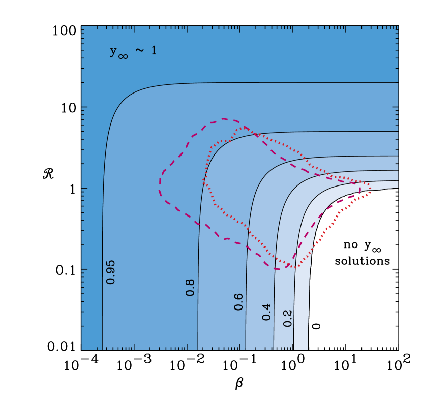
Figure 2.— Constant values of the asymptotic dimensionless frequency $y_{\infty}$ shown as labeled contours vs.  $\beta$ and ${\cal R}$. Wind measurement outlines are shown for data presented by Hellinger et al. (2006) (magenta dashed curve) and Maruca et al. (2012) (red dotted curve).

3.2. Resonant Shell Distributions: Fits to Simulations

In a collisionless medium, the presence of cyclotron resonant waves causes ion VDFs to evolve into distinctly non-bi-Maxwellian shapes. Kennel & Engelmann (1966) and Rowlands et al. (1966) showed that VDFs undergo diffusion in velocity space along resonant surfaces described by kinetic energy conservation in the wave’s phase-speed reference frame. Thus, the shapes of these resonant “shells” as a function of $v_{\parallel}$ and $v_{\perp}$ depend on the details of the dispersion relation (see also Galinsky & Shevchenko, 2000; Isenberg et al., 2000). However, as demonstrated above, when one computes the dispersion relation in anything but the cold-plasma limit, the answer depends on the thermal spread of the particles; i.e., on the shape of the VDF itself. Finding a truly self-consistent solution for both the dispersion relation and the VDF is a nontrivial problem.

For the specific case of marginal stability ($\gamma\rightarrow 0$) in a proton–electron plasma, Isenberg (2012) and Isenberg et al. (2013) found consistent numerical solutions for both $\omega_{r}(k_{\parallel})$ and $f_{p}(v_{\parallel},v_{\perp})$. These solutions were obtained under the assumption that the density of protons in velocity space decreases from its maximum central value with a specified parameterization. Nevertheless, the VDF was constrained to remain constant along the resonant shells that were consistent with the dispersion relation. The resulting dependence of ${\cal R}$ on $\beta$ was found to produce better agreement with the observed upper-right edge of the data envelopes shown in Figure 2 than did earlier results based on bi-Maxwellians.

Although solar wind protons are not likely to spend all of their time right at marginal stability, it is useful to explore how the VDF solutions of Isenberg et al. (2013) can be applied to large-scale models of cyclotron heating in the heliosphere. The dispersion relations shown in Figure 2 of Isenberg et al. (2013) were reproduced by finding a parameterized fit, which we first estimated with

$$(\Theta x)^{2}\,=\,\frac{y^{2}}{|1-y|^{\phi}}\,\,,$$ (22)

where

$$\phi\,=\,\frac{1+5\beta^{0.4}}{1+9\beta^{0.4}}$$ (23)

and $\Theta$ is defined in Equation (20). When $\beta\rightarrow 0$, the exponent $\phi$ approaches 1 and $\Theta\approx 1$, and thus Equation (22) comes into agreement with Equation (14). A simpler version of this equation (with $\phi=1$ for all values of $\beta$) was used by Isenberg (1984b) to account for both warm-plasma anisotropy effects at low wavenumber ($y\approx\Theta x$) and the cold plasma dispersion relation’s approach to $y=1$ at high wavenumber.

However, the dispersion relation given by Equations (22)–(23) does not accurately replicate the results of Isenberg et al. (2013) near the cyclotron resonance at $y\approx 1$. Once the frequency gets close to this limiting value, the self-consistent models were seen to approach it with exponential rapidity. We adjusted the solution by first solving for $y(x)$ using the above fitting formulae and calling it $y_{\rm old}$, then we forced the exponential behavior with

$$y_{\rm new}=1-(1-y_{\rm old})e^{-\alpha|x|^{3}}\,\,,$$ (24)

where $\alpha=0.22\beta^{0.5}$. The constant value of 0.22 was slightly smaller than what would be needed to reproduce the tabulated $\alpha$ values of Isenberg et al. (2013), but it worked best to reproduce the shape of the dispersion relation. Figure 3 shows the same example dispersion curves from Isenberg et al. (2013), but now computed with the above procedure. The $\Theta$ parameter was computed in each case from the tabulated pairs of $\beta$ and ${\cal R}$ listed in Table 1 of Isenberg et al. (2013).

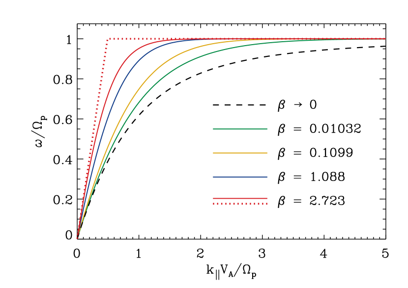
Figure 3.— Dispersion curves meant to reproduce Figure 2 of Isenberg et al. (2013). The cold plasma dispersion relation (black dashed curve) is compared with solutions to Equations (22)–(24), with labels describing the color of each curve based on $\beta$. Also shown is one example of the approximate hot dispersion relation of Equation (25) (red dotted curve).

In the high-$\beta$ limit, the solutions shown in Figure 3 appear to be approaching a kind of “hot” dispersion relation, which remains close to linear ($y\propto x$) until $y$ approaches unity, then it flattens rapidly to $y=1$ for all higher wavenumbers. The consequences of two forms of such a hot dispersion relation will be explored further below. The high-$\beta$ limit of our fit to the Isenberg et al. (2013) results is described approximately by

$$y\,=\,\min\left(\Theta x,1\right)\,\,,$$ (25)

and this is also plotted for comparison in Figure 3 for the case with the largest $\beta$. We will also explore the consequences of an even simpler hot approximation,

$$y\,=\,\min\left(x,1\right)$$ (26)

which transitions from the ideal MHD dispersion relation to strict cyclotron resonance for $x>1$.

3.3. Resonant Shell Distributions: Analytic Approximation

It is worthwhile to investigate whether a purely analytic approach to describing resonant shell VDFs could give rise to an improved dispersion relation. For the case studied below, the resulting dispersion relation turns out to be identical to the warm bi-Maxwellian approximation of Equation (18). However, we present this analysis for the sake of completeness, and to show that some fully kinetic models may sometimes give results not so different from those found by assuming bi-Maxwellian VDFs.

The major simplifying assumption made here is that the resonant shells are described by contours of constant phase speed $V_{\rm A}$ for forward and backward moving Alfvén waves. This is consistent with the ideal MHD dispersion relation ($y=x$) or, equivalently, Equation (26) above. Our goal is to determine to what extent the dispersion relation that results from solving Equation (3) is consistent with that input assumption. The proton VDFs are constant along contours described by constant values of

$$\eta^{2}\,=\,v_{\perp}^{2}+(V_{\rm A}+|v_{\parallel}|)^{2}-V_{\rm A}^{2}$$ (27)

(e.g., Isenberg, 2012), and we use the absolute value of $v_{\parallel}$ to create a symmetric VDF consistent with the presence of an equal population of forward and backward moving Alfvén waves. The normalization used in Equation (27) implies that $\eta$ is the value of $v_{\perp}$ encountered by each shell contour when it passes through $v_{\parallel}=0$.

Following Isenberg et al. (2013), the VDF is defined as a Gaussian function of the single parameter $\eta$, and the “thermal speed” in units of $\eta$ is specified as $\sigma$. The bulk thermal properties of the VDF can be parameterized in terms of a dimensionless velocity ratio $a=V_{\rm A}/\sigma$. We normalize the distribution by requiring its zeroth moment to be the proton number density, and

$$f_{p}(\eta)\,=\,\frac{n_{p}\,e^{-a^{2}}}{\pi^{3/2}\sigma^{3}(1-\mbox{erf}\,a)}\exp\left(-\frac{\eta^{2}}{\sigma^{2}}\right)\,\,,$$ (28)

where erf is the error function. In the limit of $a\rightarrow 0$, Equation (28) becomes the standard isotropic Maxwellian distribution.

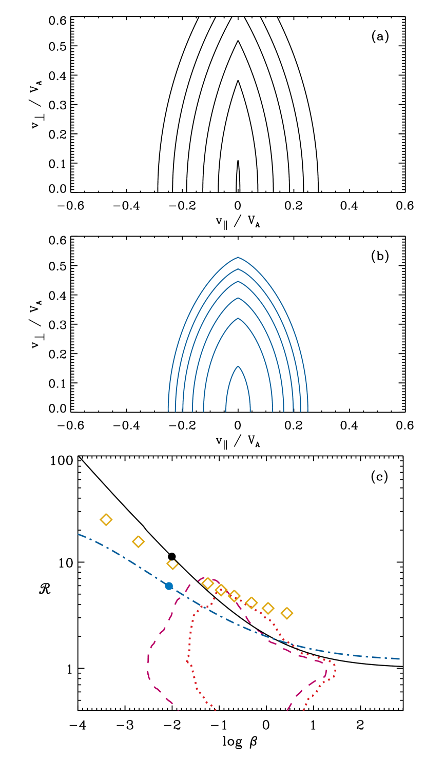
Figure 4.— Contours of $f_{p}(v_{\parallel},v_{\perp})$ for (a) the analytic model described by Equation (28) with $a=3$, and (b) resonant shell contours consistent with cold plasma dispersion, for $\beta=0.01$. (c) Loci of points in ($\beta$,${\cal R}$) space consistent with the analytic shell model (black solid curve) and the cold plasma model (blue dot-dashed curve), with the specific values of $\beta$ shown in panels (a)–(b) labeled by filled circles. Also shown are observational outlines (same as in Figure 2) and the self-consistent results of Isenberg et al. (2013) (gold diamonds).

Figure 4(a) shows contours of the VDF described above for a representative value of $a=3$. The VDF exhibits ${\cal R}>1$ anisotropy for any value of $a>0$. The moments of Equation (28) were computed in order to determine how $\beta$ and ${\cal R}$ depend on the single parameter $a$. We found that

$$w_{p\perp}^{2}=\sigma^{2}\,\,,\,\,\,\,\,w_{p\parallel}^{2}=\sigma^{2}\Psi\,\,,$$ (29)

where

$$\Psi=2a^{2}+1-\frac{2ae^{-a^{2}}}{\pi^{1/2}(1-\mbox{erf}\,a)}\,\,,$$ (30)

and thus ${\cal R}=1/\Psi$ and $\beta=\Psi/a^{2}$. For the case $a=3$ shown in Figure 4(a), the VDF exhibits $\beta=0.01203$ and ${\cal R}=9.237$. Because both ${\cal R}$ and $\beta$ are functions of a single parameter $a$, they trace out a distinct curve in the beta–anisotropy diagram.

Figure 4(b) shows a comparable set of VDF contours that were computed to be consistent with the cold plasma dispersion relation (Equation (14)); see Section 4.2 for more details about how this was done. In comparison to the dispersionless VDF shown in Figure 4(a), the cold plasma contours are known to be “snubbed” around $v_{\parallel}\approx 0$, and thus the cold VDF exhibits less anisotropy for similar values of $\beta$. Figure 4(c) illustrates the locus of points in the beta–anisotropy plane described by the above analytic model. For $\beta<1.6$, the analytic anisotropy ratio exceeds that of the cold plasma model. It also exceeds the self-consistent marginal anisotropy ratio computed by Isenberg et al. (2013) for $\beta\lesssim 0.02$.

Isenberg (2012) showed how the operator $\hat{\Sigma}$ can be written in terms of a single partial derivative of $\eta$, and we applied that expression to Equation (1). For a pure proton–electron plasma with cold (Maxwellian) electrons and $V_{\rm A}\ll c$, the dispersion relation is given by

$$\mbox{Re}(\epsilon)\,=\,\left(\frac{\omega_{pp}}{\omega_{r}}\right)^{2}\,\left\{-\frac{\omega_{r}}{\Omega_{p}}+\xi_{0}\left[S_{+}(\xi_{1},a)+S_{-}(\xi_{1},a)\right]\right.$$

$$\left.+\,a\left[S_{+}(\xi_{1},a)-S_{-}(\xi_{1},a)\right]\right\}$$ (31)

where the resonance factors are defined for the present model as

$$\xi_{0}\,=\,\frac{\omega_{r}}{k_{\parallel}\sigma}\,\,\,,\,\,\,\,\,\,\xi_{1}\,=\,\frac{\omega_{r}-\Omega_{p}}{k_{\parallel}\sigma}$$ (32)

and we define the components of a generalized plasma dispersion function as follows,

$$S_{\pm}(\xi,a)\,=\,\frac{\pm 1}{\sqrt{\pi}(1-\mbox{erf}\,a)}\int_{0}^{\pm\infty}\frac{dt\,e^{-(a+|t|)^{2}}}{t-\xi}\,\,.$$ (33)

In the limit of $a\rightarrow 0$, the sum $S_{+}+S_{-}$ becomes the standard Maxwellian dispersion function $Z(\xi)$. The difference $S_{+}-S_{-}$ does not contribute to the dispersion relation in the $a\rightarrow 0$ limit because it is multiplied by a factor of $a$ in Equation (31).

The asymptotic series expansion for large values of $|\xi|$ was obtained for $S_{+}(\xi,a)$, and the antisymmetry property

$$S_{-}(\xi,a)\,=\,-S_{+}(-\xi,a)$$ (34)

was used to compute $S_{-}(\xi,a)$. Unlike Equation (17), which has nonzero coefficients for only the odd powers of $\xi$, the full expansion for Equation (33) also has nonzero values for the even powers, with

$$S_{+}(\xi,a)\,=\,-\frac{1}{2\xi}+\frac{1}{\xi^{2}}\left(\frac{a}{2}-X\right)-\frac{1}{\xi^{3}}\left(\frac{2a^{2}+1}{4}-aX\right)$$

$$+\,\frac{1}{\xi^{4}}\left[\frac{2a^{3}+3a}{4}-(1+a^{2})X\right]+\,\cdots\,\,,$$ (35)

where $X=e^{-a^{2}}/[2\pi^{1/2}(1-\mbox{erf}\,a)]$. In Equation (31), each $1/\xi^{2n}$ (even) term ends up having a comparable contribution to the dispersion relation as the next higher $1/\xi^{2n+1}$ (odd) term, so we truncated the above series expansion at $1/\xi^{3}$. Including those terms into Equation (31), the dispersion relation was found to be

$$y^{2}=x^{2}(1-y)\left[1+\frac{y-1+\Psi}{2a^{2}(y-1)^{3}}\right]\,\,.$$ (36)

However, when the definitions of $\beta$ and ${\cal R}$ given above are substituted in for $\Psi$ and $a$, the result is seen to be identical to the bi-Maxwellian warm plasma relation of Equation (18). Interesting as that may be, it is formally inconsistent with the initial assumption of $y=x$ used to compute the VDF shell shapes. This kind of analytic model deserves further study, but for now we set it aside and follow other approaches to model the resonant diffusion of protons in velocity space.

4. Proton Cyclotron Heating

Once the dispersion relation for parallel-propagating Alfvén waves has been specified, it becomes possible to estimate the rate of energy transfer between the waves and the particles. Section 4.1 defines the relevant wave power quantities needed to determine how rapidly the protons are energized, and Sections 4.2–4.3 present two different theoretical frameworks for modeling the heating. Section 4.4 compares various estimates of the total heating rate with one another and with observational constraints.

4.1. Alfvénic Power Spectrum

For linear Alfvén waves, we assume the total energy density $U_{\rm A}$ is divided between transverse kinetic and magnetic fluctuations. The full three-dimensional (3D) power spectrum $E_{\rm A}({\bf k})$ is written as a general function of vector wavenumber ${\bf k}$ and is normalized such that

$$U_{\rm A}\,=\,\frac{1}{2}\rho_{0}\langle\delta v_{\perp}^{2}\rangle+\frac{\langle\delta B_{\perp}^{2}\rangle}{8\pi}\,=\,\int d^{3}{\bf k}\,E_{\rm A}({\bf k})\,\,.$$ (37)

The kinetic fluctuation strength depends on the background density $\rho_{0}$ and the transverse velocity variance $\langle\delta v_{\perp}^{2}\rangle$, and the associated magnetic fluctuation variance is given by $\langle\delta B_{\perp}^{2}\rangle$. The variables defined here are similar, but not identical, to those used by Cranmer & van Ballegooijen (2003, 2012).

As summarized in Section 2, we assume the low-wavenumber part of the spectrum—which contributes nearly all the power—is the product of an ongoing MHD turbulent cascade. This paper is not concerned much with that dominant part of the spectrum except as a potential source of the high-$k_{\parallel}$ ion cyclotron resonant waves. There is no agreement on the origin of the cyclotron waves, but for now we follow Chandran (2005) and Cranmer & van Ballegooijen (2012) and assume they arise from nonlinear mode coupling between Alfvén waves and compressive magnetosonic waves. In that model, the resulting Alfvénic power spectrum is close to isotropic, with a $k^{-3/2}$ reduced power-law behavior consistent with several models and simulations (e.g., Iroshnikov, 1963; Kraichnan, 1965; Nakayama, 1999; Boldyrev, 2006; Grappin et al., 2013). In order to normalize the total power to Equation (37), this kind of isotropic spectrum can be written as

$$E_{\rm A}(k)\,=\,\frac{\langle\delta B_{\perp}^{2}\rangle}{32\pi^{2}k_{0}^{3}}\,\times\left\{\begin{array}[]{ll}0\,\,,&k<k_{0}\,\,,\\ (k_{0}/k)^{7/2}\,\,,&k\geq k_{0}\\ \end{array}\right.$$ (38)

where $k_{0}$ is a representative “outer scale” wavenumber. For simplicity, we assumed equipartition between the magnetic and kinetic fluctuations.

When working with parallel-propagating ion cyclotron waves, it is not necessary to specify the full 3D power spectrum. A reduced one-dimensional spectrum (i.e., a function of $k_{\parallel}$ only) can be defined by integrating $E_{\rm A}$ over the $k_{\perp}$ coordinate. By convention, we define the reduced power spectrum $P_{\rm B}(k_{\parallel})$ as following only the magnetic fluctuations, and thus it should be normalized to

$$\frac{\langle\delta B_{\perp}^{2}\rangle}{8\pi}\,=\,\int dk_{\parallel}\,P_{\rm B}(k_{\parallel})\,\,.$$ (39)

It is also consistent with our assumption of nearly parallel-propagating waves to replace the wavenumber magnitude $k$ in Equation (38) by $k_{\parallel}$. Making that approximation, the reduced power spectrum can be written as

$$P_{\rm B}(k_{\parallel})\,\approx\,\frac{\langle\delta B_{\perp}^{2}\rangle}{48\pi k_{0}}\,\times\left\{\begin{array}[]{ll}0\,\,,&k_{\parallel}<k_{0}\,\,,\\ (k_{0}/k_{\parallel})^{3/2}\,\,,&k_{\parallel}\geq k_{0}\,\,.\\ \end{array}\right.$$ (40)

The above expression does not apply to the low-$k$ nonresonant part of the spectrum, so its integral over all values of $k_{\parallel}$ does not match up with the normalization of Equation (39). However, Equation (40) gives the proper value of the local reduced power (in the high-$k_{\parallel}$ regime) in agreement with the 3D spectrum of Equation (38).

Another way to normalize the reduced power spectrum is to specify its value at the nominal proton cyclotron resonant wavenumber $k_{\parallel}=\Omega_{p}/V_{\rm A}$ (i.e., $x=1$). Calling this normalized power level $P_{1}$, a simple parameterization is given by

$$P_{\rm B}(k_{\parallel})\,=\,P_{1}\left(\frac{\Omega_{p}}{k_{\parallel}V_{\rm A}}\right)^{n}\,=\,\frac{P_{1}}{x^{n}}\,\,,$$ (41)

where we normally assume $n=3/2$ as above. In typical models of the solar corona and heliosphere (e.g., Cranmer & van Ballegooijen, 2012), the resonant wavenumber $\Omega_{p}/V_{\rm A}$ is many orders of magnitude larger than the turbulent energy-containing wavenumber $k_{0}$. Although Equation (41) is used for most of the proton heating models described below, it is occasionally compared with Equation (40) in order to estimate a reasonable range of values for $P_{1}$.

The above expressions assumed $k_{\parallel}>0$ for outward propagating waves. However, the models below sometimes include a population of inward propagating waves (i.e., $k_{\parallel}<0$) as well. When evaluating the power available for these waves, we first specify the power in outward waves, then set the inward wave power as a specified fraction $f_{\rm in}$ of the outward power. Thus, the limiting case of purely outward propagating waves corresponds to $f_{\rm in}=0$, and the case of balanced power between outward and inward modes (i.e., zero cross-helicity) corresponds to $f_{\rm in}=1$. Details about the power spectrum for the inward waves are computed from expressions such as Equations (40) or (41), but with the absolute value of $k_{\parallel}$ or $x$ used instead of the signed quantity. The sign of $k_{\parallel}$ matters in the resonance factors and diffusion coefficients described below.

Lastly, we note that the power-law spectra described above do not contain the effects of wave dissipation that are caused by the wave-particle interactions. These effects have been included in phenomenological models of turbulent cascade (e.g., Li et al., 2001; Howes et al., 2008; Jiang et al., 2009; Cranmer & van Ballegooijen, 2012). Section 5 treats spectral damping for the specific problem of alpha particles sapping away the energy before the protons have a chance to resonate with the high-$k_{\parallel}$ fluctuations. However, for the models discussed in the remainder of this section we continue to assume a power-law form of $P_{\rm B}(k_{\parallel})$ for simplicity.

4.2. Quasilinear Diffusion in Velocity Space

The derivation of the linear dispersion relation made the assumption that fluctuations in the VDFs and electromagnetic fields are small first-order oscillations, and that any second- or higher-order quantities are negligible. To determine how the waves and particles interact with one another to produce net heating, a so-called quasilinear approach is often applied (Kennel & Engelmann, 1966; Rowlands et al., 1966; Galeev & Sagdeev, 1983; Marsch & Tu, 2001a). In quasilinear theory, second-order fluctuation quantities are retained and averaged over spatial and time scales long in comparison to those of the gyromotions, and random phases are assumed for the first-order Fourier oscillations themselves.

Following Marsch & Tu (2001a), the zeroth-order VDF $f_{s}(v_{\parallel},v_{\perp})$ for ion species $s$ evolves via diffusion in velocity space, with

$$\frac{\partial f_{s}}{\partial t}\,=\,\frac{1}{v_{\perp}}\frac{\partial}{\partial v_{\perp}}\left[v_{\perp}\left(D_{\perp\perp}\frac{\partial f_{s}}{\partial v_{\perp}}+D_{\perp\parallel}\frac{\partial f_{s}}{\partial v_{\parallel}}\right)\right]$$

$$+\,\frac{\partial}{\partial v_{\parallel}}\left(D_{\parallel\perp}\frac{\partial f_{s}}{\partial v_{\perp}}+D_{\parallel\parallel}\frac{\partial f_{s}}{\partial v_{\parallel}}\right)\,\,.$$ (42)

The diffusion coefficients are given by

$$\left\{\begin{array}[]{c}D_{\parallel\parallel}\\ D_{\parallel\perp}\\ D_{\perp\perp}\\ \end{array}\right\}=\left(\frac{2\pi q_{s}}{m_{s}c}\right)^{2}\!\!\int\!dk_{\parallel}\frac{P_{\rm B}(k_{\parallel})}{k_{\parallel}^{2}}\,\Gamma_{\rm res}(v_{\parallel},k_{\parallel})\left\{\begin{array}[]{c}k_{\parallel}^{2}v_{\perp}^{2}\\ k_{\parallel}v_{\perp}\Omega_{\ast}\\ \Omega_{\ast}^{2}\\ \end{array}\right\}$$ (43)

and $D_{\parallel\perp}=D_{\perp\parallel}$. There is some disagreement in the literature about the identity of the frequency-like variable $\Omega_{\ast}$. Melrose (1986) and Marsch & Tu (2001a) give $\Omega_{\ast}=\Omega_{s}$, but Lee (1971) and Isenberg & Vasquez (2007) give $\Omega_{\ast}=\omega_{r}-k_{\parallel}v_{\parallel}$. These two formulations are identical to one another when the resonance factor $\Gamma_{\rm res}$ is a Dirac delta function (see below). For now we continue to follow Marsch & Tu (2001a) and assume $\Omega_{\ast}=\Omega_{s}$ (see also Equations 2.29–2.31 of Kennel & Engelmann (1966)), but in future work we will explore whether the use of the other definition produces qualitatively different results.

In the standard weak-damping limit of quasilinear theory, the cyclotron resonance factor $\Gamma_{\rm res}$ is defined as

$$\Gamma_{\rm res}(v_{\parallel},k_{\parallel})\,=\,\delta(\omega_{r}-k_{\parallel}v_{\parallel}-\Omega_{s})$$ (44)

and applying this Dirac delta function to Equation (43) transforms the integration over $k_{\parallel}$ into a trivial selection of a single resonant wavenumber. For parallel propagating waves obeying a single-branch dispersion relation with $\omega_{r}\lesssim\Omega_{p}$, it is usually the case that $v_{\parallel}<0$ is required for proton resonance with outward propagating waves and $v_{\parallel}>0$ is needed for resonance with inward propagating waves. When those conditions do not apply, the argument of the delta function is never zero no matter the value of $k_{\parallel}$, so there is thought to be no diffusion in those parts of velocity space.

It is sometimes overlooked that Equation (44) is an approximate limiting case of a more general resonance factor that applies for arbitrary values of $\gamma$, the imaginary part of the frequency. The general version is given by

$$\Gamma_{\rm res}(v_{\parallel},k_{\parallel})\,=\,\frac{|\gamma/\pi|}{\gamma^{2}+(\omega_{r}-k_{\parallel}v_{\parallel}-\Omega_{s})^{2}}$$ (45)

and it tends toward the limit of a Dirac delta function as $\gamma\rightarrow 0$. Gary & Saito (2003) noted that particle-in-cell simulations of proton cyclotron diffusion exhibit a smearing effect in $v_{\parallel}$ that could be due to the fact that $\gamma\neq 0$. Nonresonant regions of velocity space that exhibit no nonzero solutions to Equation (44) instead exhibit a small—but not negligible—diffusion coefficient due to the more spread-out nature of Equation (45).

In order to evaluate Equation (45), we estimated $\gamma(k_{\parallel})$ by using a weak-damping approximation that is often applied in tandem with quasilinear theory,

$$\frac{\gamma}{\omega_{r}}\,=\,-\frac{\mbox{Im}(\epsilon)}{2\,\,\mbox{Re}(\epsilon)}$$ (46)

with $\mbox{Re}(\epsilon)=k_{\parallel}^{2}c^{2}/\omega_{r}^{2}$ and

$$\mbox{Im}(\epsilon)\,=\,-\frac{4\pi^{3}}{\omega_{r}^{2}k_{\parallel}}\sum_{s}\frac{q_{s}^{2}}{m_{s}}\int dv_{\perp}\,v_{\perp}^{2}\left(\Omega_{s}\frac{\partial f}{\partial v_{\perp}}+k_{\parallel}v_{\perp}\frac{\partial f}{\partial v_{\parallel}}\right)_{\rm res}\,\,.$$ (47)

The subscript “res” constrains the quantity in parentheses to be evaluated at the value of $v_{\parallel}$ that satisfies the resonance condition $\omega_{r}-k_{\parallel}v_{\parallel}-\Omega_{s}=0$. This is not fully self-consistent, since it implicitly uses the delta function assumption of Equation (44), but it represents an iterative step toward an improved solution. When computing $\gamma$, we used only the proton contribution to the sum over particle species $s$. This component of the damping rate is often written as $\gamma_{p}$.

Figure 5 shows example calculations of the magnitude of the diffusion coefficient $D_{\perp\perp}$ as a function of $v_{\parallel}$ (here computed for $v_{\perp}=0$). These curves were computed for purely outgoing waves ($f_{\rm in}=0$) obeying the cold plasma dispersion relation and an isotropic Maxwellian proton VDF with $\beta=0.1$ As expected, the idealized delta function resonance factor gives rise to finite values of $D_{\perp\perp}$ only for $v_{\parallel}<0$. However, the more accurate version (Equation (45)) produces nonzero values of $D_{\perp\perp}$ for all values of $v_{\parallel}$. Figure 5 also shows how the diffusion coefficient approaches the appropriate $\gamma\rightarrow 0$ limit when the damping rate is multiplied by a range of arbitrary reduction factors.

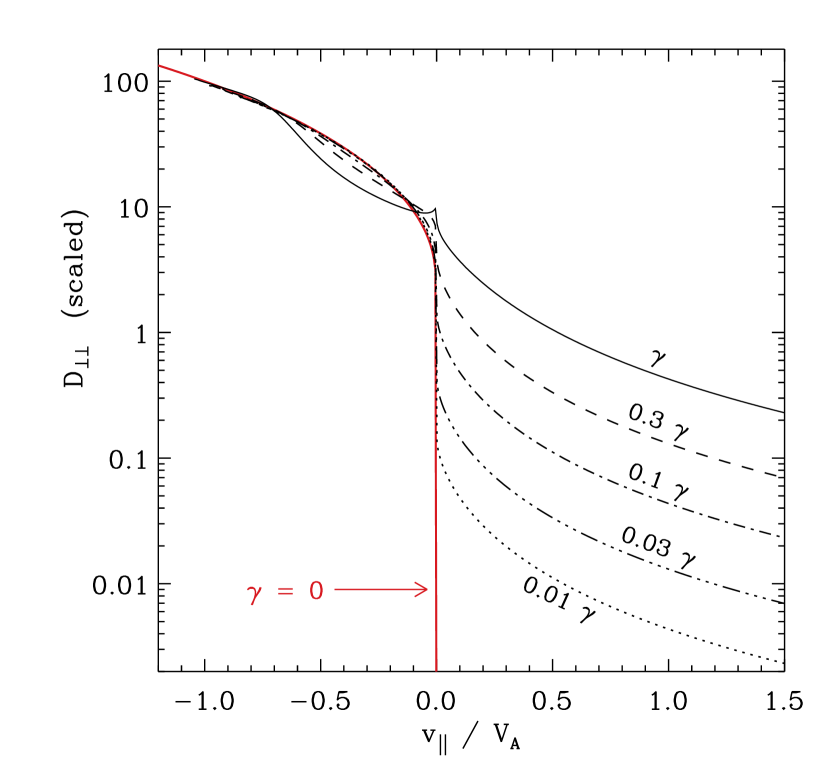
Figure 5.— Scaled diffusion coefficient $D_{\perp\perp}$ plotted vs.  parallel velocity $v_{\parallel}$, computed with various approximations for the damping rate $\gamma$. The result of Equation (44) (red solid curve) is compared with that of Equation (45) for both the actual estimated value of $\gamma(k_{\parallel})$ (black solid curve) and a range of artificially reduced damping rates (see curve labels for reduction factors).

In Figure 5 there is a small cusp of increased diffusivity around $v_{\parallel}=0$ for the model with no reduction in $\gamma$. The behavior of $D_{\perp\perp}$ at this velocity depends on the high-$k_{\parallel}$ (i.e., $x\gg 1$) limiting behavior of both the dispersion relation and the power spectrum $P_{\rm B}$. This calculation was done with the power-law version of $P_{\rm B}$ described by Equation (40). Presumably, if the damping implied by our computed value of $\gamma$ was applied self-consistently to the high-wavenumber part of the power spectrum, the appearance of this cusp would be significantly muted.

The diffusion coefficients describe the shapes of resonant shell contours in velocity space toward which the VDF should evolve as $t\rightarrow\infty$ in Equation (42). At any given value of $v_{\parallel}$ and $v_{\perp}$, one can estimate the local angle $\alpha$ between the shell contour and the $v_{\parallel}$ axis as

$$\tan\alpha\,\approx\,\frac{D_{\parallel\perp}}{D_{\parallel\parallel}}\,\,.$$ (48)

Figure 4(b) shows the result of tracing out these contours for an example proton VDF with $\beta=0.01$ and waves obeying the cold plasma dispersion relation. This calculation assumed Equation (44) for outward propagating waves resonant with $v_{\parallel}<0$ protons, and the shell shapes were reflected around $v_{\parallel}=0$ to show the contours for inward propagating waves resonant with $v_{\parallel}>0$ protons. As described above, the cold plasma dispersion relation gives rise to marginally stable proton VDFs that are more isotropic than if the shell shapes were computed with ideal MHD dispersion (shown in Figure 4(a)).

Equation (42) is solved numerically with a similar explicit finite differencing technique as that of Cranmer (2001). The standard benchmark case discussed below is a pure proton–electron plasma with waves obeying the cold dispersion relation. The initial condition is always a bi-Maxwellian proton VDF. The numerical diffusion code recomputes $\gamma(k_{\parallel}$) at each time step using Equation (46). The code runs slowly when using Equation (45) for every calculation of $\Gamma_{\rm res}$, since in this case the full integration over $k_{\parallel}$ must be performed numerically. Thus, the results shown below were obtained by using Equation (44) in resonant regions of velocity space (i.e., where there exist values of $k_{\parallel}$ that satisfy the proton resonance condition $\omega_{r}-k_{\parallel}v_{\parallel}-\Omega_{p}=0$) and Equation (45) elsewhere. In order that the solutions for $\Gamma_{\rm res}$ be continuous as a function of $v_{\parallel}$, we also used Equation (45) in resonant regions of velocity space with $|v_{\parallel}|\leq w_{p\parallel}$.

Figure 6 illustrates the time evolution of proton VDFs computed by the numerical diffusion code. Two runs are shown, both with initial conditions of $\beta=0.01$ and ${\cal R}=1$. The upper set of panels shows the evolution with $f_{\rm in}=0$ (all outward wave power), and the lower set shows the result of assuming $f_{\rm in}=1$ (balanced outward and inward power). The evolution time is specified in units of a characteristic timescale $\tau_{d}$ for perpendicular diffusion, with

$$\tau_{d}\,=\,w_{p\perp}^{2}/D_{\perp\perp}\,\,,$$ (49)

where $D_{\perp\perp}$ is evaluated at the peak of the initial VDF ($v_{\parallel}=v_{\perp}=0$) at $t=0$. The explicit nature of the finite differencing technique necessitated the use of a small time step of order $10^{-3}\tau_{d}$.

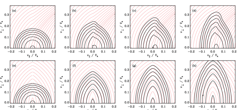
Figure 6.— Contour plots of the proton VDF (black curves) shown at four times in its evolution. From left to right, $t=0$, 0.24, 0.48, and 2.4 in units of $\tau_{d}$. The models assumed $f_{\rm in}=0$ (top row) and $f_{\rm in}=1$ (bottom row). VDF contours are separated by constant factors of 0.5 in $\log f_{p}$. Red dotted contours show sets of resonant shells computed by tracing streamlines using Equation (48). For clarity, in the bottom row we show only the “dominant” set of resonant shells in each half of velocity space.

The VDFs shown in Figure 6 initially approach the marginally stable shell contours (red dotted curves) that we estimated from Equation (48), but they appear later to diffuse into more perpendicularly anisotropic shapes. The VDF of the model with $f_{\rm in}=0$ resembles the numerical results of Gary & Saito (2003). In nonresonant parts of velocity space, the quasi-resonant shell contours that we found by tracing the $\alpha$ angle have roughly hyperbolic shapes. This causes the initially isotropic VDF in the $v_{\parallel}>0$ region to diffuse into the perpendicular direction—despite the absence of a classical resonance condition there—and for the peak of the VDF to migrate to a slightly higher value of $v_{\parallel}$ as well.

The model with balanced inward and outward wave power (lower panels of Figure 6) undergoes substantial additional diffusion because of the existence of resonant shells that cross over one another. Isenberg (2001) suggested this could give rise to augmented perpendicular heating akin to the stochastic energization found in second-order Fermi acceleration. More surprisingly, our model with $f_{\rm in}=0$ (upper panels) appears to undergo extra diffusion of this type as well. This is likely to be the result of the “spreading” inherent in Equation (45), such that the resonant contours represent merely the centroids of a range of possible diffusion pathways in velocity space.

Additional information about the quasilinear diffusion in these models can be seen by plotting the time dependence of the VDF moments $w_{p\parallel}$ and $w_{p\perp}$. Hollweg (1999) discussed the conditions for net perpendicular heating and parallel cooling of protons in resonance with cyclotron waves. Figure 7(a) illustrates this evolution for the two models discussed above and an intermediate model with $f_{\rm in}=0.5$. The initial rates of heating and cooling are faster for the models with inward propagating waves, since the total power present in the system is proportional to $1+f_{\rm in}$. Thus, it is not surprising that the model with $f_{\rm in}=1$ has roughly twice as steep an initial slope as the model with $f_{\rm in}=0$. The models with additional inward power not only evolve more rapidly, but they also begin to approach larger asymptotic values of $w_{p\perp}$ and $w_{p\parallel}$ because of the Fermi-like effect discussed above.

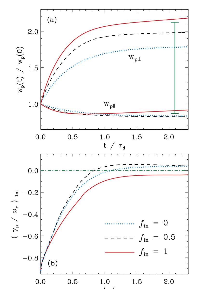
Figure 7.— Time evolution of (a) thermal speed moments $w_{p\perp}$ (upper curves) and $w_{p\parallel}$ (lower curves) normalized to their initial values, and (b) the wavenumber integrated damping rate defined by Equation (50). In both panels, the models correspond to $f_{\rm in}=0$ (blue dotted curve), $f_{\rm in}=0.5$ (black dashed curve), and $f_{\rm in}=1$ (red solid curve). In the upper panel, the green strut illustrates the magnitude of the “filled-shell” anisotropy ratio from the corresponding model shown in Figure 4(b).

Figure 7(b) shows the time evolution of a wavenumber-integrated damping rate

$$\left(\frac{\gamma}{\omega_{r}}\right)_{\rm tot}\,=\,\frac{V_{\rm A}}{\Omega_{p}}\int dk_{\parallel}\,\,\frac{\gamma(k_{\parallel})}{\omega_{r}(k_{\parallel})}$$ (50)

(see also Cranmer, 2001). The isotropic initial condition undergoes substantial wave damping consistent with the rapid evolution to higher anisotropy. The $f_{\rm in}=0$ model approaches an asymptotic steady state with a positive (unstable) value of $(\gamma/\omega_{r})_{\rm tot}$ because its $v_{\parallel}>0$ shells never become completely “filled” in a marginally stable way. On the other hand, the $f_{\rm in}=1$ model remains stable for the entire simulation and evolves monotonically toward an asymptotic state with net damping. It is interesting that the subsequent Fermi-like diffusion away from the resonant shells shown in Figure 6 is still consistent with a stable late-time evolution with $\gamma<0$. The model with $f_{\rm in}=0.5$ first becomes even more unstable than the other two models, but eventually the Fermi-like diffusion occurs and drives $(\gamma/\omega_{r})_{\rm tot}$ slowly back down to $\gamma\approx 0$.

The numerical diffusion models shown above followed the proton VDFs from their initial state in ($\beta$,${\cal R}$) space to an asymptotic final state near the marginal stability curve. However, a truly self-consistent model should have recalculated the dispersion relation (which depends on the evolving VDF shape) at each time step. In lieu of tackling this extremely complex problem (see, e.g., Isenberg, 2012; Isenberg et al., 2013), we now limit ourselves to measuring only the initial rates of change away from the VDF at $t=0$. This may be a more practical way of studying how the system evolves when it is far from the marginal stability curve. Following earlier work such as Arunasalam (1976), the rates of net heating or cooling are defined as

$$\left\{\begin{array}[]{c}Q_{p\parallel}\\ Q_{p\perp}\\ \end{array}\right\}\,=\,n_{p}k_{\rm B}\frac{\partial}{\partial t}\left\{\begin{array}[]{c}T_{p\parallel}/2\\ T_{p\perp}\\ \end{array}\right\}$$ (51)

such that their sum is the time rate of change of the total proton internal energy density ($3n_{p}k_{\rm B}T_{p}/2$). The one-fluid proton temperature is defined as $T_{p}=(T_{p\parallel}+2T_{p\perp})/3$, and the partial time derivatives are assumed to apply only for early times $t\ll\tau_{d}$.

Figure 8 shows contours of the early-time heating rates computed for a range of initial bi-Maxwellian VDFs. The upper panels show the fully bi-Maxwellian approximation described in Section 4.3, and the lower panels show a coarser (11 $\times$ 13) grid of results of the numerical diffusion code discussed above. The plotted quantity is a dimensionless version of the heating/cooling rate,

$$I_{p\parallel,\perp}\,=\,\frac{V_{\rm A}\,Q_{p\parallel,\perp}}{4P_{1}\Omega_{p}^{2}}\,\,.$$ (52)

For the numerical diffusion models, a cold plasma dispersion relation with pure outward waves ($f_{\rm in}=0$) was assumed. The heating rates were computed by fitting the evolution of $w_{p\parallel}^{2}(t)$ and $w_{p\perp}^{2}(t)$ with linear slopes. Each case was run for 50 time steps, where one time step was given roughly by $10^{-5}\tau_{d}$. At these early times, there were no significant deviations from linear increases/decreases in $w_{p\parallel}^{2}$ and $w_{p\perp}^{2}$.

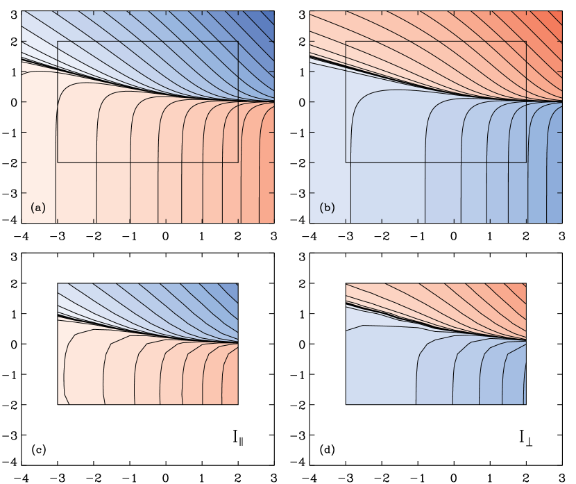
Figure 8.— Contours of the signed, dimensionless heating rates $I_{p\parallel}$ (left panels) and $I_{p\perp}$ (right panels). Parameter values are given by the color bar at bottom, and the solid black contours are separated from their neighbors by multiplicative factors of 4. Panels (a)–(b) show bi-Maxwellian solutions of Equation (53) and panels (c)–(d) show numerical VDF diffusion results from Equation (51). The square box in the upper panels highlights the subset of parameter space spanned by the models in the lower panels.

Note from Figures 8(c)–(d) that the two-dimensional ($\beta$,${\cal R}$) space is divided by the so-called marginal stability curve. “Below” that curve (i.e., for the lowest values of ${\cal R}$, including ${\cal R}=1$), $I_{p\parallel}$ is negative and $I_{p\perp}$ is positive. The opposite is the case above the curve. Thus, the net effect of cyclotron heating is to drive a plasma either up from below or down from above, in this diagram, to approach marginal stability as an asymptotic final state. The curve that defines $I_{p\parallel}=0$ is not identical to the curve that defines $I_{p\perp}=0$. However, these two loci remain sufficiently close to one another that they can be described more or less as a single curve. Their degree of relative separation depends slightly on the properties of the dispersion relation (see below).

4.3. Bi-Maxwellian Heating and Cooling Rates

If the proton VDFs are assumed to always have a bi-Maxwellian shape as described by Equation (4), the velocity-space diffusion coefficients and the derivatives in Equation (42) can be evaluated explicitly as functions of $T_{p\parallel}$ and $T_{p\perp}$ (e.g., Marsch & Tu, 2001a). With this assumption, the heating and cooling rates can be written

$$\left\{\begin{array}[]{c}Q_{p\parallel}\\ Q_{p\perp}\\ \end{array}\right\}\,=\,-4\int dk_{\parallel}\,P_{\rm B}(k_{\parallel})\,\frac{\gamma_{p}}{\omega_{r}}\left\{\begin{array}[]{c}\omega_{r}-\Omega_{p}\\ \Omega_{p}\\ \end{array}\right\}\,\,,$$ (53)

where the bi-Maxwellian version of the proton damping rate is given by

$$\frac{\gamma_{p}}{\omega_{r}}\,=\,-\frac{\pi^{1/2}e^{-\xi_{1}^{2}}}{2}\left(\frac{\Omega_{p}}{k_{\parallel}V_{\rm A}}\right)^{2}\left({\cal R}\xi_{1}+\frac{\Omega_{p}}{k_{\parallel}w_{p\parallel}}\right)\,\,,$$ (54)

and $\xi_{1}$ is the resonance factor defined in Equation (8). A dimensionless form of the heating rates is given by

$$\left\{\begin{array}[]{c}I_{p\parallel}\\ I_{p\perp}\\ \end{array}\right\}\,=\,-\int\frac{dx}{x^{n}}\left(\frac{\gamma_{p}}{\omega_{r}}\right)\left\{\begin{array}[]{c}y-1\\ 1\\ \end{array}\right\}\,\,,$$ (55)

where $x$ and $y$ are the scaled wavenumber and frequency variables defined in Equation (10), and $n$ is the power spectrum exponent that we tend to fix at 3/2.

Figures 8(a)–(b) show the result of solving Equation (55) on a fine two-dimensional grid of $\beta$ and $\cal R$ values. As above, we assumed a cold plasma dispersion relation with $f_{\rm in}=0$. For each point in the grid, the wavenumber integral over $x$ was computed on a logarithmic scale from $x=10^{-3}$ to $10^{+3}$. The smallest values of $x$ tend not to contribute to the integral because $\gamma_{p}$ grows exponentially small for $x\ll 1$, and the largest values of $x$ do not contribute because of the power spectrum falloff of $x^{-n}$. A comparison of the upper and lower panels of Figure 8 shows that the bi-Maxwellian heating rates are always quite similar in magnitude to the heating rates computed from the numerical VDF diffusion model. This may not be surprising, since the numerical models above were computed only for early times when the VDF presumably remains close to its initial bi-Maxwellian shape. Nevertheless, these early-time rates may be the most appropriate ones to use when studying how the plasma state evolves across wide swaths of the ($\beta$,${\cal R}$) diagram. The remainder of this paper will assume bi-Maxwellian VDFs for computing $I_{p\parallel}$ and $I_{p\perp}$.

The models shown in Figure 8 were computed assuming outward waves only (i.e., $f_{\rm in}=0$). However, the appearance of these contours would not be all that different had other values of $f_{\rm in}$ been utilized (as long as the total wave power was normalized in a consistent way). Thus, in the bi-Maxwellian models described below we will use $f_{\rm in}=0$ and assume that the effects of inward resonances can be taken into account by increasing the wave power quantity $P_{1}$.

For a given set of model assumptions, the marginal stability curve can be estimated to be the locus of points where either $Q_{p\parallel}=0$ or $Q_{p\perp}=0$. One can also define a curve on which there is a zero rate of change in the anisotropy ratio ${\cal R}$. For the model of cyclotron heating studied here, this latter curve always falls in between the two (already closely spaced) curves that denote $Q_{p\parallel}=0$ and $Q_{p\perp}=0$. Thus, we choose to use this condition, with

$$\frac{\partial{\cal R}}{\partial t}\,=\,\frac{Q_{p\perp}-2{\cal R}Q_{p\parallel}}{n_{p}k_{\rm B}T_{\parallel}}\,=\,0\,\,,$$ (56)

as a practical concordance definition of marginal stability for the bi-Maxwellian heating model.

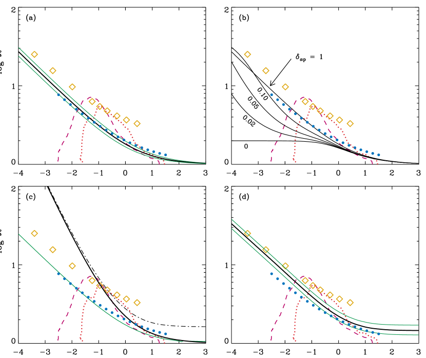
Figure 9.— Theoretical marginal stability curves compared in each panel with measurements at 1 AU (red and magenta curves; see Figure 2), numerical results of Isenberg et al. (2013) (gold diamonds), and the parallel cyclotron instability threshold of Maruca et al. (2012) (blue filled circles). Specific model parameters for the four panels (black and green curves) are enumerated in the text.

Figure 9 shows marginal stability curves defined by $\partial{\cal R}/\partial t=0$ for a range of different dispersion relations, power spectrum indices, and alpha–proton relative velocities. Each of these curves was extracted from a full grid of heating rates $I_{p\parallel}$ and $I_{p\perp}$, similar to the ones shown in Figure 8(a)–(b). These different cases also exhibit modest differences in the magnitudes of the heating rates away from marginal stability; this will be explored further in Section 6.2. The specific models included in the four panels of Figure 9 are described below.

1. Figure 9(a) shows marginal stability curves computed with a cold plasma dispersion relation, no alpha particles, and a range of power spectrum exponents $n=0.5$, 1.5, and 3. Larger values of $n$ correspond to lower threshold values of ${\cal R}$ for marginal stability, but the curves do not move up or down by very much from the standard intermediate case of $n=1.5$ (thick black curve). These models correspond rather closely to the marginal stability curve of Maruca et al. (2012) that was computed using a numerical Vlasov–Maxwell dispersion code with bi-Maxwellian proton VDFs (blue symbols).

2. Figure 9(b) shows the result of using the cold proton–alpha dispersion relation given by Equation (16), with $n=1.5$, $h=0.05$, and a range of relative drift speeds $\delta_{\alpha p}$. The largest value of $\delta_{\alpha p}=1$ corresponds to the alpha particles being fully out of resonance. Thus, its curve is indistinguishable from the corresponding curve in Figure 9(a). When $\delta_{\alpha p}$ approaches zero, the marginal stability curve moves down to substantially lower values of ${\cal R}$. This occurs because the smaller frequency on the lower proton–alpha dispersion branch (Figure 1(a)) makes a major change in the boundary between regions of positive and negative $I_{p\parallel}$ (see Equation (55)).

3. Figure 9(c) explores the result of utilizing the warm and hot dispersion relations derived in Sections 3.1–3.2. From bottom to top, the curves show the bi-Maxwellian warm dispersion relation (Equation (18); green solid curve), the simplest version of the hot dispersion relation (Equation (26); thick black curve), and the hot dispersion relation with anisotropic pressure (Equation (25); black dot-dashed curve). These calculations assumed $h=0$ and $n=1.5$. The warm dispersion curve is nearly identical to that computed with the cold plasma dispersion relation, and also with the numerical results of Maruca et al. (2012). However, the curves computed with the hot dispersion relations extend to substantially higher values of ${\cal R}$ than are seen in other models. For $-1.3\lesssim\log\beta\lesssim-0.6$, the hot curves agree well with the upper edge of the measured range of anisotropy ratios.

4. Figure 9(d) shows marginal stability curves computed from our fits to the Isenberg et al. (2013) dispersion relations, as described by Equations (22)–(24). The three curves show a range of power spectrum exponents $n=0.5$, 1.5, and 3, with larger values of $n$ corresponding to lower values of ${\cal R}$ as in Figure 9(a). At low values of $\beta$, these curves closely approach the numerical results of Isenberg et al. (2013) (gold diamonds). At high values of $\beta$, the models disagree with the numerical results but still approach an asymptotic value of ${\cal R}>1$ similar to the hot anisotropic model shown in Figure 9(c). Both of those models have dispersion relations that reduce to $y\approx\Theta x$ in the limit of high $\beta$ and low $k_{\parallel}$.

The diversity of curve shapes in Figure 9 is somewhat surprising, since all of these results were computed from dispersion relations built on either cold plasma or bi-Maxwellian foundations. None of them agree exactly with marginal stability curves computed from shell-shaped proton VDFs, like the numerical results of Isenberg et al. (2013) or the analytic shell model of Section 3.3 (see the black curve in Figure 4(c)). In a truly self-consistent model, the position of the marginal stability curve in the beta–anisotropy plane must evolve in time as the VDFs evolve in shape.

4.4. Total Heating Rate Comparisons

Prior to applying the above description of proton cyclotron resonance to a model of the solar wind, the absolute normalization for the heating rate (which depends on the wave power spectrum) must be specified. As discussed in Section 2, the total rate of plasma heating may be the result of several different physical processes. Thus, here we aim to explore the range of likely values for both the total heating rate and the contribution from cyclotron resonance. Figure 10 shows $Q_{p}=Q_{p\parallel}+Q_{p\perp}$ versus heliocentric distance $r$ for several assumptions about the heating. Black curves indicate the total heating rates (protons plus electrons) from the fast-wind turbulence models of Cranmer et al. (2007) and Cranmer & van Ballegooijen (2012). These compare favorably to heating rates determined from Helios and Ulysses measurements (Cranmer et al., 2009), which are also illustrated in Figure 10. These heating rates are all roughly consistent with a power-law scaling of $Q\propto r^{-4.5}$.

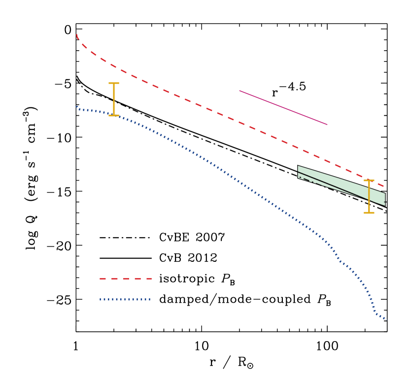
Figure 10.— Radial dependence of heating rates for various models of the fast wind. Total ($Q_{p}+Q_{e}$) rates from turbulence models of Cranmer et al. (2007) (black dot-dashed curve) and Cranmer & van Ballegooijen (2012) (black solid curve) agree with rates inferred from in situ measurements (Cranmer et al., 2009) (green region). Proton cyclotron heating rates $Q_{p}$ are also shown for an assumed isotropic wave spectrum (red dashed curve) and the damped anisotropic spectrum of Cranmer & van Ballegooijen (2012) (blue dotted curve). Ranges of imposed heating rates in the models of Section 6.3 are shown with gold bars.

Figure 10 also shows two calculations of the radial dependence of $Q_{p}$ that assumed proton cyclotron resonance is the sole source of heating. For the fast-wind (polar coronal hole) model of Cranmer & van Ballegooijen (2012)—which specifies time-steady background quantities such as $V_{\rm A}$ and $\beta$—we solved Equation (52) for $Q_{p}$. This requires knowledge of both the wave power normalization quantity $P_{1}$ and the total scaled heating rate $I_{p}=I_{p\parallel}+I_{p\perp}$. Assuming isotropic proton VDFs (${\cal R}=1$), the only other parameter that causes $I_{p}$ to vary is $\beta$. We extracted this dependence from the model illustrated in Figure 8 and fit it with

$$\log I_{p}\,\approx\,-0.324+0.227\log\beta+0.0168(\log\beta)^{2}\,\,\,\,\,\,(\mbox{for}\,\,{\cal R}=1).$$ (57)

To obtain the red and blue curves in Figure 10, $P_{1}$ was estimated in two different ways. First, we took as an upper limit the isotropic power spectrum model of Equation (40), with the quantities $\langle\delta B_{\perp}^{2}\rangle$ and $k_{0}$ taken from the wave transport model of Cranmer & van Ballegooijen (2012). This model is labeled “isotropic $P_{\rm B}$” in Figure 10, and it produces several orders of magnitude greater proton heating than is inferred to exist in the fast wind. This result is consistent with the results of Isenberg & Vasquez (2011), who found that one needs only $\sim 10^{-2}$ of the total available wave power to be in the form of high-$k_{\parallel}$ cyclotron waves in order to heat the protons adequately.

On the other hand, the blue curve labeled “damped/mode-coupled $P_{\rm B}$” was computed using the full Cranmer & van Ballegooijen (2012) model for the Alfvénic power spectrum in the corona and heliosphere. This model contained an anisotropic cascade, with only a small fraction of the total wave energy reaching the high-$k_{\parallel}$ cyclotron resonance. In Figure 10, we plot only the proton heating rate due to cyclotron wave damping, but the original model also contained proton heating due to Landau and transit-time resonances. Because the high-$k_{\parallel}$ waves were strongly depleted in this model (relative to an isotropic power spectrum), the heating rate $Q_{p}$ is much smaller than is generally believed to be needed to heat solar wind protons. A complete understanding of proton energetics is likely to require more than one source of heat. In Section 6 we assume that $Q_{p\parallel}$ and $Q_{p\perp}$ are given by linear combinations of terms from cyclotron resonance and an unspecified second source that, for simplicity, we assume heats the protons isotropically.

5. The Effect of Drifting Alpha Particles

When multiple ion species are present in a plasma containing cyclotron resonant waves, it is possible for some ions to block others from receiving the full extent of the heating they would have received in isolation. This effect has been studied extensively for the case of alpha particles preventing the protons from being heated resonantly (e.g., Liewer et al., 2001; Xie et al., 2004; Gary et al., 2005; Maneva et al., 2013; Kasper et al., 2013). Also, Cranmer (2000, 2001) found that even minor ions (with, e.g., $n_{i}/n_{p}$ as low as $\sim$10^-5) may be efficient at absorbing high-$k_{\parallel}$ waves that propagate up from the solar surface and become resonant high in the corona. A main conclusion from these studies has been that some kind of gradual replenishment of the wave spectrum—such as from a turbulent cascade—is needed to explain how the protons may be heated in this way. Sometimes, however, the resonant damping may be so rapid that even an efficient cascade may not be able to supply wave power to the protons. The goal of this section is to estimate the degree to which proton heating rates ($Q_{p\parallel}$, $Q_{p\perp}$) are suppressed by the presence of alpha particles.

The models described in Section 4 assumed a power-law form for $P_{\rm B}(k_{\parallel})$. Here, we aim to take into account the high-$k_{\parallel}$ damping due to both protons and alphas in a more self-consistent way. We follow Cranmer & van Ballegooijen (2012) and assume the “replenishment” of the Alfvénic fluctuation spectrum comes from an isotropic cascade of fast-mode waves that are locally mode-converted into Alfvén waves. This last step is assumed to be relatively instantaneous, which enables us to combine the effects of cascade and damping into a single transport equation for the Alfvénic power spectrum. This transport equation is written in terms of the full 3D power spectrum $E_{\rm A}({\bf k})$ to retain continuity with the equations of Cranmer & van Ballegooijen (2012).

In the past, turbulent cascades have been modeled as a combination of wavenumber advection (i.e., first-order transport that goes strictly from low to high $k$) and diffusion (i.e., second-order transport that spreads out the power in both directions, but ends up ultimately with a turbulent power law). Many aspects of the transport do not depend on the relative strengths of the advection and diffusion terms, so for simplicity we assume pure advection (see also Appendix C.2 of Cranmer & van Ballegooijen (2012)). Thus, the proposed transport equation, for an isotropic cascade in $k$, is given by

$$\frac{\partial E_{\rm A}}{\partial t}\,=\,-\frac{\mu}{k^{2}}\frac{\partial}{\partial k}\left(\frac{k^{3}E_{\rm A}}{\tau_{c}}\right)+2\gamma E_{\rm A}\,\,.$$ (58)

The first term on the right-hand side describes the wavenumber advection, where $\mu$ is an order-unity constant and $\tau_{c}$ is a $k$-dependent cascade timescale given by

$$\tau_{c}\,=\,\frac{V_{\rm A}}{kv^{2}}\,=\,\frac{\rho_{0}V_{\rm A}}{k^{4}E_{\rm A}}\,\,.$$ (59)

Equation (59) assumes that the timescale is constrained by the weak Iroshnikov–Kraichnan type cascade experienced by fast-mode waves prior to being coupled back to the Alfvén mode. The spectrum of velocity fluctuations $v(k)$ is related to the energy spectrum as $\rho_{0}v^{2}=k^{3}E_{\rm A}$.

The second term on the right-hand side of Equation (58) produces damping when $\gamma<0$. We assume that the resonant waves of interest are sufficiently close to parallel propagation that $k\approx k_{\parallel}$. The 1D transport equation is then solved by integrating from an initial condition at an outer-scale wavenumber $k_{0}$. This wavenumber is assumed to be far below the scales at which the resonant damping occurs. Thus, for a time-steady system ($\partial E_{\rm A}/\partial t=0$), the solution of Equation (58) is

$$E_{\rm A}(k)=E_{0}\left(\frac{k_{0}}{k}\right)^{7/2}+\frac{\rho_{0}V_{\rm A}}{\mu k^{7/2}}\int_{k_{0}}^{k}\frac{dk}{k^{3/2}}\,\gamma(k)\,\,,$$ (60)

where $E_{0}$ is defined as the known power level at $k_{0}$, and it is related to the root-mean-squared fluctuation velocity via $k_{0}^{3}E_{0}=\rho_{0}\langle\delta v_{\perp}^{2}\rangle$. Using the equations from Section 4.1, the 1D reduced power spectrum is given by $P_{\rm B}=2\pi k_{\parallel}^{2}E_{\rm A}/3$.

Equation (60) exhibits an undamped inertial range at low wavenumbers, and it steepens to an infinitely sharp asymptote near the point at which the cascade timescale equals the inverse damping rate (i.e., $|\gamma\tau_{c}|\approx 1$). This transition from the inertial range to the dissipation range appears to model the expected behavior of the system reasonably well, despite the fact that the solution for $E_{\rm A}$ at even larger wavenumbers is negative and unphysical. For convenience, we express this solution dimensionlessly by dividing by the inertial range solution,

$$\widetilde{E}\,\equiv\,\frac{E_{\rm A}}{E_{0}(k_{0}/k)^{7/2}}\,=\,1\,+\,C\int_{x_{0}}^{x}\frac{y\,\,dx}{x^{3/2}}\left(\frac{\gamma}{\omega_{r}}\right)$$ (61)

where as above we define $x=k_{\parallel}V_{\rm A}/\Omega_{p}$ and $y=\omega_{r}/\Omega_{p}$. The key constant that sets the level of relative “competition” between cascade and damping is $C$, which is defined as

$$C\,=\,\frac{8\pi V_{\rm A}^{2}}{\mu\langle\delta v_{\perp}^{2}\rangle}\left(\frac{\Omega_{p}}{k_{0}V_{\rm A}}\right)^{1/2}\,\,.$$ (62)

Note that $C$ can also be written as the product of $\Omega_{p}$ and a representative cascade timescale that applies at $x\approx 1$. In the solar wind, $C\gg 1$ because $k_{0}$ is always several orders of magnitude smaller than the resonant wavenumber $\Omega_{p}/V_{\rm A}$. Also, $V_{\rm A}^{2}\gg\langle\delta v_{\perp}^{2}\rangle$ in the corona, but these velocities are of the same order of magnitude at larger heliocentric distances. Using the fast solar wind model of Cranmer & van Ballegooijen (2012), we assumed $\mu=2$ and we computed $C$ as a function of distance. In the low corona, $C\gtrsim 10^{6}$, and it declines rapidly to $\sim 10^{5}$ at $r=4\,R_{\odot}$, to $\sim 10^{4}$ at $r=20\,R_{\odot}$, and to $\sim 10^{3}$ at $r=5$ AU.

Figure 11 shows how the damping rates and resulting spectra change when the helium abundance $h$ and relative drift speed $\delta_{\alpha p}$ are varied. The damping rate $\gamma$ is computed by solving Equation (46), assuming bi-Maxwellian VDFs for both protons and alpha particles, and Equation (16) was used for the real part of the dispersion relation. In Figure 11, the parameters held fixed are $\beta=0.01$, $C=10^{4}$, $T_{\alpha}/T_{p}=4$, and ${\cal R}=1$ for both protons and electrons. Because of the lower charge-to-mass ratio of the alphas, they have the opportunity to undergo cyclotron resonance at lower values of $k_{\parallel}$ than do the protons.

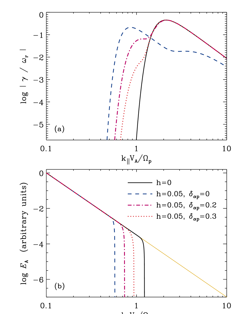
Figure 11.— (a) Absolute values of dimensionless damping rates $|\gamma/\omega_{r}|$ as a function of parallel wavenumber. (b) Damped wave spectra consistent with damping rates shown in panel (a), compared with the undamped spectrum (solid gold curve). In both panels, the result for a pure proton-electron plasma (black solid curve) is compared with that for 5% helium abundance and drift speeds $\delta_{\alpha p}=0$ (blue dashed curve), 0.2 (magenta dot-dashed curve), and 0.3 (red dotted curve).

For $\beta\ll 1$, the power spectrum computed for no alphas ($h=0$) is indistinguishable from that computed for $h=0.05$ and $\delta_{\alpha p}\approx 1$. For large drifts, the alphas become “Doppler shifted” well out of resonance and the dispersion relation is effectively that of a pure proton–electron plasma. However, at higher values of $\beta$, Verscharen et al. (2013) found that the presence of drifting alphas may destabilize the protons near $\delta_{\alpha p}\approx 1$, leading to $\gamma>0$ and the possibility of wave growth. This effect was also found in the models discussed here, but only for a narrow range of drift parameters $\delta_{\alpha p}$ extremely close to 1.

For the case of $h=0.05$ and several fixed choices of $C$, damped power spectra were computed for a large grid of values of $\beta$ and $\delta_{\alpha p}$. Each spectrum was processed through Equation (53) to obtain heating rates $Q_{p\parallel}$ and $Q_{p\perp}$. We found that a convenient dimensionless way to measure the ability of alpha particles to suppress the proton heating (as derived in Section 4) is the ratio

$${\cal D}(\beta,\delta_{\alpha p})\,=\,\frac{Q_{p\perp}(\beta,\delta_{\alpha p})}{Q_{p\perp}(\beta,1)}\,\,.$$ (63)

Since ${\cal D}\leq 1$, this ratio describes how a given level of alpha–proton drift gives rise to an additional amount of damping relative to what would occur when the alphas are fully out of resonance. The behavior for $Q_{p\parallel}$ is nearly identical to the behavior for $Q_{p\perp}$, so for simplicity we use Equation (63) for both.

Figure 12(a) shows the full dependence of ${\cal D}$ on on both $\beta$ and $\delta_{\alpha p}$ for $C=10^{4}$ (representative of the inner heliosphere) and fixed values of ${\cal R}=1$ and $T_{\alpha}/T_{p}=4$. There is a plateau of ${\cal D}\approx 1$ at low values of $\beta$ and large values of $\delta_{\alpha p}$. However, ${\cal D}$ drops precipitously as one moves from the upper-left to the lower-right part of the panel. As suspected from earlier studies (e.g., Gary et al., 2005; Bourouaine et al., 2011), alpha particles at low drift speeds capture most of the wave energy themselves and prevent the protons from being heated (i.e., ${\cal D}\approx 0$). Figure 12 also shows the dividing line given by Kasper et al. (2013), which was parameterized as

$$\delta_{\rm cut,K}\,=\,\min\left(0.168+\beta^{1/2},1\right)$$ (64)

and was proposed to account for the $\beta$-dependence of the resonant cutoff between regions of strong and weak alpha particle suppression of proton heating. This curve is quite similar in shape and position to the contours that describe the dropoff of ${\cal D}$.

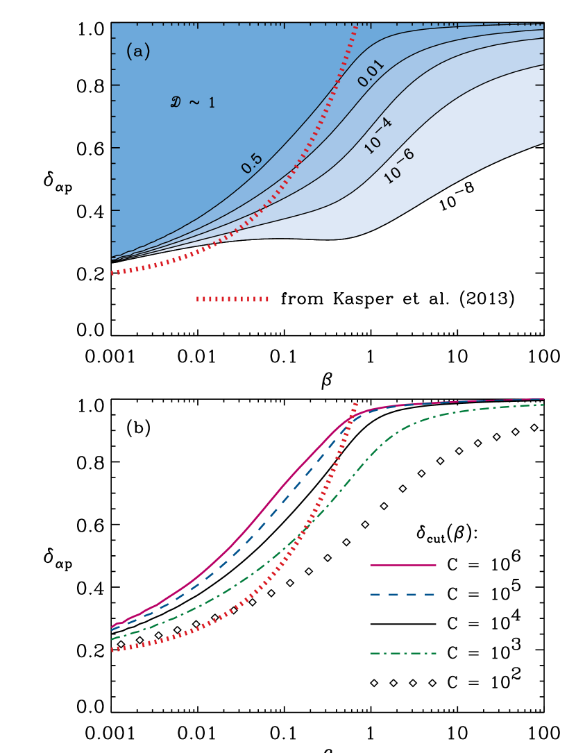
Figure 12.— (a) Contours of constant values of ${\cal D}$ as a function of proton $\beta$ and alpha–proton drift speed $\delta_{\alpha p}$, computed for $C=10^{4}$. (b) $\delta_{\rm cut}$ plotted versus $\beta$ for models computed with a range of cascade–damping constants $C$ (see labels). In both panels, the red dotted curve corresponds to Equation (64).

In order to make efficient use of the two-dimensional distributions ${\cal D}(\beta,\delta_{\alpha p})$ in spatially extended solar wind models, we parameterized these functions as follows. For a given grid of ratios like that plotted in Figure 12(a), we determined the locus of points that corresponds to the ${\cal D}=0.5$ contour. This describes a function $\delta_{\rm cut}(\beta)$ that roughly divides the grid into two regions of strong and weak alpha suppression. Figure 12(b) shows $\delta_{\rm cut}$ versus $\beta$ for several grids that were computed with different values of $C$. In addition, Table 1 provides $\delta_{\rm cut}$ for a coarse grid of $\beta$ values. Given the numerical tabulation of $\delta_{\rm cut}(\beta)$, we then represent the full dependence of ${\cal D}$ with

$${\cal D}(\beta,\delta_{\alpha p})\,\approx\,\frac{1}{2}\left[1+\mbox{erf}\left(\frac{\delta_{\alpha p}-\delta_{\rm cut}(\beta)}{\sigma_{\rm cut}}\right)\right]$$ (65)

where $\sigma_{\rm cut}=0.04$ reproduces the numerical results quite well. For simplicity, in the solar wind simulations described below we use only this model for a single intermediate value of $C=10^{4}$.

Table 1Cutoff Drift Speeds for Suppression of Proton Heating

$\beta$	$\delta_{\rm cut}$ ($C=10^{5}$)	$\delta_{\rm cut}$ ($C=10^{4}$)	$\delta_{\rm cut}$ ($C=10^{3}$)
1E–3	0.2624	0.2501	0.2327
2E–3	0.2961	0.2786	0.2572
5E–3	0.3522	0.3283	0.2978
1E–2	0.4071	0.3748	0.3365
2E–2	0.4735	0.4327	0.3818
5E–2	0.5813	0.5253	0.4556
1E–1	0.6763	0.6098	0.5234
2E–1	0.7732	0.7025	0.6011
5E–1	0.9052	0.8394	0.7235
1E+0	0.9601	0.9248	0.8206
2E+0	0.9776	0.9630	0.8928
5E+0	0.9865	0.9806	0.9412
1E+1	0.9911	0.9864	0.9588
2E+1	0.9942	0.9906	0.9692
5E+1	0.9972	0.9942	0.9778
1E+2	0.9990	0.9959	0.9820

6. Radial Evolution of the Proton Velocity Distribution

Earlier sections described how solar wind protons are energized by cyclotron resonant interactions in regions where the background plasma parameters are assumed to be fixed and homogeneous. Here we develop a larger-scale global model of how these effects may manifest themselves along flux tubes that extend from the corona ($r\approx 2\,R_{\odot}$) to interplanetary space. Section 6.1 lays out the bi-Maxwellian moment equations adopted for this model. We acknowledge that real heliospheric VDFs are never exactly bi-Maxwellian, but we wish to explore the extent to which the moment equations faithfully model the kinetic processes that dominate proton energetics in the solar wind. Results are presented first for a flux tube representative of high-latitude fast wind streams (Section 6.2), then for a broad Monte Carlo ensemble of heliospheric parameters (Section 6.3).

6.1. Conservation Equations

The radial evolution of proton VDFs is modeled here by time-steady 1D conservation equations for the bi-Maxwellian temperature parameters $T_{p\parallel}$ and $T_{p\perp}$ and a simplified equation for the alpha–proton drift parameter $\delta_{\alpha p}$. The radial dependences of proton number density $n_{p}$ and outflow speed $u_{p}$, as well as electron temperature $T_{e}$, are determined separately (see below). The temperature equations were simplified from the 16-moment model of Li (1999) and are given by

$$\frac{\partial T_{p\parallel}}{\partial r}\,=\,-T_{p\parallel}\left(\frac{2\cos^{2}\Phi}{L_{u}}+\frac{\sin^{2}\Phi}{L_{b}}\right)$$

$$+\,\frac{4\nu_{pp}}{5u_{p}}\left(T_{p\perp}-T_{p\parallel}\right)+\frac{2\nu_{pe}}{u_{p}}\left(T_{e}-T_{p\parallel}\right)+\frac{2Q_{p\parallel}}{n_{p}u_{p}k_{\rm B}}$$ (66)

$$\frac{\partial T_{p\perp}}{\partial r}\,=\,-T_{p\perp}\left(\frac{\sin^{2}\Phi}{L_{u}}+\frac{2-\sin^{2}\Phi}{2L_{b}}\right)$$

$$+\,\frac{2\nu_{pp}}{5u_{p}}\left(T_{p\parallel}-T_{p\perp}\right)+\frac{2\nu_{pe}}{u_{p}}\left(T_{e}-T_{p\perp}\right)+\frac{Q_{p\perp}}{n_{p}u_{p}k_{\rm B}}$$ (67)

(see also Isenberg & Hollweg, 1983; Cranmer et al., 1999; Matteini et al., 2012). From left to right, terms on the right-hand sides of Equations (66)–(67) describe double-adiabatic expansion, collisional isotropization, electron–proton collisional equilibration, and net heating. These equations do not include proton heat conduction, which is often found to be of negligible importance in solar wind thermodynamics (Sandbaek & Leer, 1995; Cranmer et al., 2009; Hellinger et al., 2013). Two key scale lengths used above are defined as

$$\frac{1}{L_{u}}=\frac{1}{u_{p}}\frac{\partial u_{p}}{\partial r}\,\,\,,\,\,\,\,\,\,\,\,\frac{1}{L_{b}}=-\frac{1}{B_{r}}\frac{\partial B_{r}}{\partial r}\,\,.$$ (68)

For models at low heliographic latitudes, we include the effect of the Parker spiral by defining

$$\tan\Phi\,=\,\frac{B_{\phi}}{B_{r}}\,=\,-\frac{\Omega_{s}r\sin\vartheta}{u_{1{\rm AU}}}$$ (69)

where $\vartheta$ is the colatitude of the wind streamline (usually $\pi/2$ for the ecliptic) and the solar rotation rate is $\Omega_{s}=2.7\times 10^{-6}$ rad s^-1. Equation (69) uses $u_{1{\rm AU}}$, the wind speed at 1 AU, instead of the radially varying wind speed, to better approximate the end-result of solving the full set of MHD angular momentum equations (Weber & Davis, 1967).

The proton–proton Coulomb collision rate was given by Li (1999) as

$$\nu_{pp}\,=\,\frac{4}{3}\sqrt{\frac{\pi}{m_{p}}}\frac{n_{p}e^{4}\ln\Lambda}{(k_{\rm B}T_{p})^{3/2}}\,\,,$$ (70)

with the one-fluid proton temperature defined as $T_{p}=(T_{p\parallel}+2T_{p\perp})/3$ and the Coulomb logarithm given approximately by

$$\ln\Lambda\,=\,23.2+\frac{3}{2}\ln\left(\frac{T_{p}}{10^{6}\,\mbox{K}}\right)-\frac{1}{2}\ln\left(\frac{n_{p}}{10^{6}\,\mbox{cm}^{-3}}\right)$$ (71)

(see, e.g., Cranmer et al., 2007). Similarly, the electron–proton collision rate is

$$\nu_{pe}\,=\,\frac{4}{3}\frac{\sqrt{2\pi m_{e}}}{m_{p}}\frac{n_{p}e^{4}\ln\Lambda}{(k_{\rm B}T_{e})^{3/2}}\,\,.$$ (72)

The above expressions do not take account of temperature anisotropy effects on the collision rates (see, e.g., Barakat & Schunk, 1982; Hellinger & Trávníček, 2009). A useful quantity for studying solar wind parcels at 1 AU is the dimensionless proton collisional age $A_{p}$. This quantity is often defined as the product of the proton self-collision rate and an estimate of the solar wind transit-time from the Sun to a given radius. Defining the latter as $t_{\rm wind}\approx r/u_{p}$, we define $A_{p}=\nu_{pp}t_{\rm wind}$, and we evaluate these quantities all at 1 AU. Protons in wind streams with $A_{p}\gg 1$ have experienced many collisions and should be well isotropized.

The proton heating rates $Q_{p\parallel}$ and $Q_{p\perp}$ contain the distilled results of the models developed in Sections 3–5. Figure 10 shows that various models of turbulent transport tend to produce power-law radial dependences $Q\propto r^{-n}$. The models presented below use this simple form as a starting point. Although we acknowledge that the actual heating rates must be functions of the local turbulence amplitudes, correlation lengths, and cascade rates, we also want to focus here on the relative partitioning of heat between various modes of wave-particle interaction as described above. Thus, we believe that treating the total available heat as a sum of power-law components may not be too unrealistic.

Two power-law heating components are utilized: one due to ion cyclotron resonance, and one that is assumed to heat the protons isotropically. This latter source is proposed mainly because it is a simple “null hypothesis,” not because of the existence of any single mechanism that produces isotropic heating. Still, if there exist several other heating processes in the solar wind besides ion cyclotron resonance—with multiple steps of energy conversion prior to the final step of particle heating—it may not be unrealistic to assume their summed effect provides comparable amounts of heat to $T_{p\parallel}$ and $T_{p\perp}$. The radial dependences of the two total rates are given as

$$Q_{\rm cyc}\,=\,Q_{1}\left(\frac{R_{\odot}}{r}\right)^{\psi_{1}}\,\,\,,\,\,\,\,\,\,\,Q_{\rm iso}\,=\,Q_{2}\left(\frac{R_{\odot}}{r}\right)^{\psi_{2}}$$ (73)

where the normalizing constants $Q_{1}$ and $Q_{2}$ and the exponents $\psi_{1}$ and $\psi_{2}$ are free parameters. Once these are specified, the parallel and perpendicular heating rates are

$$Q_{p\parallel}\,=\,\frac{Q_{\rm cyc}{\cal D}I_{p\parallel}}{|I_{p\parallel}+I_{p\perp}|}+\frac{Q_{\rm iso}}{3}$$ (74)

$$Q_{p\perp}\,=\,\frac{Q_{\rm cyc}{\cal D}I_{p\perp}}{|I_{p\parallel}+I_{p\perp}|}+\frac{2Q_{\rm iso}}{3}$$ (75)

where $I_{p\parallel}$ and $I_{p\perp}$ are specified by Equation (55) and ${\cal D}$ is given by Equation (65). The factors of $1/3$ and $2/3$ in the $Q_{\rm iso}$ terms are there to ensure that $T_{p\parallel}$ and $T_{p\perp}$ would receive equal rates of increase if there were no other heating or cooling terms in Equations (66)–(67).

To avoid a proliferation of free parameters, the exponent $\psi_{2}$ is set to a constant value of 4.5. This is consistent with the implicit assumption that $Q_{\rm iso}$ is dominated by the dissipation of a perpendicular KAW cascade (see Figure 10). The other three parameters ($\psi_{1}$, $Q_{1}$, $Q_{2}$) are varied freely in the models. In practice, however, we select $Q_{1}$ and the value of $Q_{\rm cyc}$ at 1 AU, and then solve for the value of $\psi_{1}$ that connects them with a power law. The kinetic effects of cyclotron wave damping and instability are included in Equations (74)–(75) because both $I_{p\parallel}$ and $I_{p\perp}$ depend on the local values of ${\cal R}$ and $\beta$ as illustrated in Figure 8. The effect of the firehose instability is not included explicitly in $Q_{p\parallel}$ and $Q_{p\perp}$, but in Section 6.2 we discuss an approximate method of computing its net impact on the proton VDF.

The dimensionless alpha–proton drift parameter $\delta_{\alpha p}$ should be determined from a complete solution of the coupled momentum transport equations for $u_{\alpha}$ and $u_{p}$. For now, however, we make a first step in this direction by solving a simpler radial evolution equation. This equation contains only the collisional friction that is expected to produce a steady decrease in $\delta_{\alpha p}$; i.e., it starts at a specified initial condition in the corona, and it is driven toward zero in the limit of a strongly collisional history. The differential momentum equation of Hernández et al. (1987) was adapted into the following form,

$$\frac{\partial}{\partial r}\left(\ln\delta_{\alpha p}\right)\,=\,-\frac{\nu_{\alpha p}}{u_{p}}\left[\frac{\mbox{erf}(\zeta)-2\zeta e^{-\zeta^{2}}/\sqrt{\pi}}{\zeta^{3}}\right]$$ (76)

where an effective drift Mach number is defined as

$$\zeta\,=\,\delta_{\alpha p}V_{\rm A}\left(\frac{2k_{\rm B}T_{\alpha}}{m_{\alpha}}+\frac{2k_{\rm B}T_{p}}{m_{p}}\right)^{-1/2}$$ (77)

and the frictional collision rate is

$$\nu_{\alpha p}\,=\,16\sqrt{2}\,\nu_{pp}\,\left(\frac{T_{\alpha}}{T_{p}}+4\right)^{-3/2}\,\,.$$ (78)

When $\zeta\ll 1$, the square-bracket term in Equation (76) approaches a constant value of $\sim$0.752. When $\zeta\gg 1$ (i.e., the runaway regime), the term in square brackets declines as $1/\zeta^{3}$. As above, we assume $T_{\alpha}/T_{p}=4$ to evaluate the above terms. Conveniently, in this limit, $\nu_{\alpha p}=\nu_{pp}$.

Equations (66), (67), and (76) are integrated from low to high $r$ with straightforward first-order Euler steps. We chose a lower boundary of $r=2\,R_{\odot}$ at which the proton VDF is assumed to be isotropic and in collisional equilibrium with the electron VDF. Thus, the lower boundary condition is that $T_{p\parallel}=T_{p\perp}=T_{e}$, where the latter is given by an empirical parameterization that agrees reasonably well with coronal and in situ measurements,

$$T_{e}\,=\,\frac{10^{6}\,\,\mbox{K}}{0.3(r/R_{\odot})^{0.6}\,+\,(r/R_{\odot})^{-1}}\,\,.$$ (79)

This expression has a maximum value of $\sim$1.1 MK at $r\approx 2.9\,R_{\odot}$, and it decreases slowly to about 0.13 MK at 1 AU. The lower boundary condition on the alpha–proton drift parameter is fixed at $\delta_{\alpha p}=1$, which assumes strong differential acceleration of heavy ions in the corona, as inferred from coronagraph spectroscopy (Kohl et al., 2006).

At heliocentric distances above 2 $R_{\odot}$, the radial magnetic field strength is reasonably approximated by a spherically expanding flux tube, with $B_{r}\propto r^{-2}$ and thus $L_{b}=r/2$. The azimuthal field strength $B_{\phi}$ was computed from Equation (69) and the vector magnitude $B_{0}=(B_{r}^{2}+B_{\phi}^{2})^{1/2}$ was used in the definitions of $V_{\rm A}$ and $\Omega_{p}$. The solar wind is still undergoing significant acceleration in the regions around $r=2\,R_{\odot}$, so it was not reasonable to assume a constant value of $u_{p}$. We found that the low-latitude solar wind models of Cranmer et al. (2013) all exhibited a roughly similar relative acceleration profile above 2 $R_{\odot}$, which we fit by a simple function

$$\frac{u_{p}(r)}{u_{1{\rm AU}}}\,=\,0.062+0.938\left(1-\frac{R_{\odot}}{r}\right)^{5.1}\,\,.$$ (80)

An actual model of $u_{p}(r)$ is then obtained by choosing a normalizing value of $u_{1{\rm AU}}$, which we do either by an explicit choice or by sampling from a random probability distribution. The derivative of Equation (80) is used to find the radial dependence of $L_{u}$. Lastly, mass flux conservation is used to obtain the radial dependence of density. We set its absolute value by choosing the sphere-averaged mass loss rate $\dot{M}$, and at 1 AU the density is computed as

$$\rho_{1{\rm AU}}\,=\,\frac{\dot{M}}{(4\pi u_{p}r^{2})_{1{\rm AU}}}\,\,.$$ (81)

At other heights, $\rho(r)$ obtained from the assumption that $\rho u/B_{r}$ remains constant. For the models described below, we assumed $h=0.05$ and we converted between mass density and proton number density with $\rho=m_{p}n_{p}(1+4h)$.

6.2. Results: Fast Solar Wind

To begin exploring how the conservation equations behave when the anisotropic heating rates are varied, we set the background solar wind conditions to those appropriate for a high-speed stream connected to a polar coronal hole (see, e.g., Section 2.1 of Cranmer & van Ballegooijen, 2012). Specifically, we set $u_{1{\rm AU}}=750$ km s^-1, $B_{r,1{\rm AU}}=3$ nT, and $\dot{M}=2\times 10^{-14}$ $M_{\odot}$ yr^-1. All other parameters were determined as described in Section 6.1.

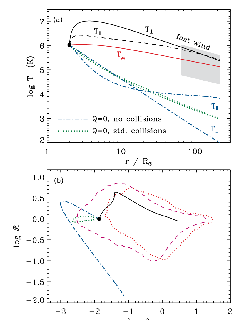
Figure 13.— (a) Radial dependence of $T_{p\parallel}$ and $T_{p\perp}$ for fast-wind models, shown together with (b) associated curves in ($\beta$,${\cal R}$) space. Initial conditions shown as black circles. Proton temperatures computed with strong heating (black curves) are contrasted with models computed for $Q_{p}=0$ with no collisions (blue dot-dashed curves) and for $Q_{p}=0$ with standard collision rates (green dotted curves). Also shown is the empirical $T_{e}$ (red solid curve). A gray region in (a) encloses the full range of $T_{p}$ variation seen by Helios, and red/magenta regions in (b) show the range of Wind data at 1 AU.

Figure 13(a) shows the radial dependence of $T_{p\parallel}$ and $T_{p\perp}$ for several cases, and Figure 13(b) shows corresponding trajectories in the beta–anisotropy plane. As has been known for several decades (e.g., Hartle & Sturrock, 1968), a complete lack of proton heating gives rise to proton temperatures well below the measured values at 1 AU. When the full Coulomb self-collision terms are used in Equations (66)–(67), the low temperatures produced in the $Q_{p}=0$ model give large values of $\nu_{pp}$. Thus, the system is rapidly driven toward isotropy, and the radial decrease in temperature is close to adiabatic ($T_{p}\propto r^{-4/3}$). In this case, Figure 13(b) shows that the $\beta$ ratio does not vary substantially on its journey from the corona to interplanetary space, and in fact at 1 AU it loops back to nearly its initial value.

Figure 13 also shows the result of turning off all Coulomb collisions for the model with $Q_{p}=0$. With neither heating nor collisional isotropization, the proton VDF obeys strict magnetic moment conservation and is beamed to a state of ${\cal R}\ll 1$ at 1 AU (e.g., Hollweg, 1971; Leer & Axford, 1972; Denton et al., 1994). An even more idealized case of a constant wind speed, a radial field, and no Parker spiral would produce $T_{p\parallel}=\mbox{constant}$ and $T_{p\perp}\propto r^{-2}$. This is close to what is seen in the blue curves of Figure 13(a) above $r\approx 10\,R_{\odot}$.

Lastly, Figure 13 shows the result of applying realistic proton heating parameters that were chosen to reproduce the median Helios fast-wind measurements reported by Marsch et al. (1982). These conditions were notable because the temperatures were near the high end of the full range of observed conditions, and they exhibited ${\cal R}>1$ at 0.3 AU and ${\cal R}<1$ at 1 AU. The three parameters that reproduce this state were found to be $Q_{1}=1.596\times 10^{-6}$ erg s^-1 cm^-3, $\psi_{1}=4.150$, and $Q_{2}=1.660\times 10^{-6}$ erg s^-1 cm^-3. To generate the observed conditions, the model needed to have $Q_{\rm cyc}/Q_{\rm iso}\approx 1$ in the corona, and then this ratio needed to increase to about 6 at 1 AU. Figure 13(b) shows that this model’s coronal evolution follows the left edge of one of the Wind beta–anisotropy regions (Maruca et al., 2012). At larger distances, the strong heating is necessary to drive the model to larger values of $\beta$ as seen in the data. For this model, $\delta_{\alpha p}$ decreased only negligibly from its initial value of 1 to a value of 0.973 at 1 AU. Below, we find that the more dominant slow/dense solar wind undergoes a much stronger heliospheric decline in $\delta_{\alpha p}$.

The strongly heated fast-wind model shown in Figure 13 exhibits a total heating rate at 1 AU of $Q_{p}=3.87\times 10^{-16}$ erg s^-1 cm^-3, which falls comfortably within the uncertainty limits of the rates computed from in situ data by Vasquez et al. (2007) and Cranmer et al. (2009). The agreement with coronal observations is not so good; the model gives a maximum value of $T_{p\perp}\approx 10$ MK in the extended corona, whereas the Ultraviolet Coronagraph Spectrometer (UVCS) instrument on the Solar and Heliospheric Observatory (SOHO) allowed for no more than $T_{p\perp}\approx 3$ MK (Kohl et al., 2006). Note, however, that our use of a lower boundary condition at $r=2\,R_{\odot}$ may be the cause of unrealistic conditions in the first few solar radii above the surface. We experimented with using a smaller initial radius, but a proper model with $r<2\,R_{\odot}$ would necessitate the use of departures from the power-law heating rates given in Equation (73).

Although none of the three models displayed in Figure 13 ventured into the firehose-unstable region in the lower-right part of the ($\beta$,${\cal R}$) plane, other models are likely to do so. Thus, for the results shown below we augment the solution algorithm for $T_{p\perp}(r)$ in a way that accounts for this instability. Matteini et al. (2012) and Seough et al. (2013) showed that if the system is driven to a point below the curve of marginal firehose stability, the net effect of the instability will be to heat up $T_{p\perp}$ and leave $T_{p\parallel}$ relatively unchanged. Thus, for $\beta>2$ we impose a lower limit on the perpendicular temperature that demands

$$T_{p\perp}\,\geq\,\left(1-\frac{2}{\beta}\right)T_{p\parallel}$$ (82)

(see Section 3.1 and Figure 2). If the locally computed value of $T_{p\perp}$ ever violates the above condition, we replace it with the lower-limit value that depends on $\beta$ and $T_{p\parallel}$. This is similar to the techniques employed by Sharma et al. (2006) and Chandran et al. (2011). Equation (82) is consistent with the classical nonresonant firehose instability, but similar expressions taken from calculations of the resonant parallel or oblique firehose instability (Gary et al., 1998; Rosin et al., 2011; Maruca et al., 2012; Michno et al., 2014) could also be used.

In order to illustrate how the solutions depend on the heating parameters $Q_{1}$, $\psi_{1}$, and $Q_{2}$, we created several grids of models in which each of the parameters is varied independently of the others. Figure 14 shows a selection of these model results in the ($\beta$,${\cal R}$) plane. It should be made clear that these curves do not show radial variations (like in Figure 13) but instead give the conditions at 1 AU that result from smoothly varying the heating parameters. Different points along each curve correspond to models with different values of either $Q_{1}$ or $Q_{2}$, and an increase in one of the heating rates tends to push the solutions from left to right in the diagram.

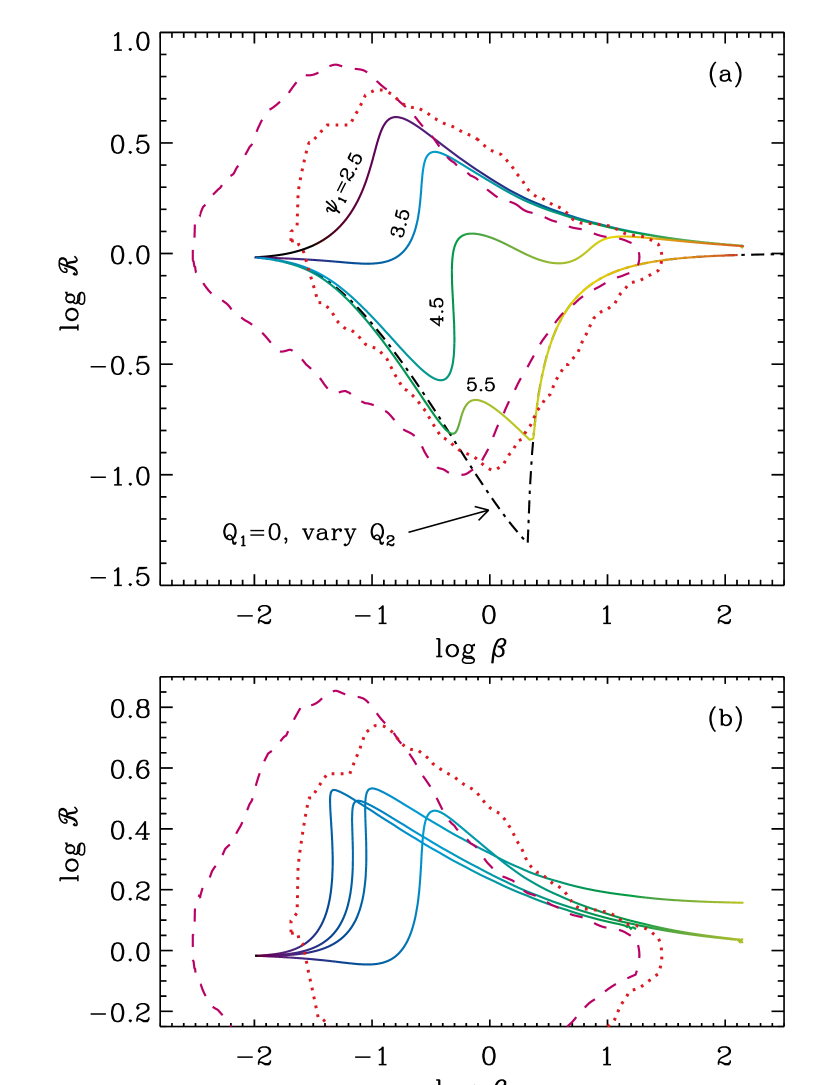
Figure 14.— Fast-wind results at 1 AU in the beta–anisotropy plane. (a) Multicolor curves have variable $Q_{1}$ and fixed values of $\psi_{1}$ (see labels and color bar) and also assume $Q_{2}=0$. Black dot-dashed curve has variable $Q_{2}$ and assumes $Q_{1}=0$. All curves in (a) use Equation (26) for the dispersion relation. (b) Multicolor curves have variable $Q_{1}$, $\psi_{1}=3.5$, and $Q_{2}=0$. From left to right (in the nearly vertical parts of the curves), the corresponding dispersion relations are Equations (18), (15), (22), and (26).

We point out several properties of these models:

1. The multicolor curves in Figure 14(a) show the result of varying $Q_{1}$ and fixing $Q_{2}=0$. In other words, they show that it is possible to populate nearly the entire observed region of the beta–anisotropy plane at 1 AU by including only proton cyclotron resonant heating and a sufficiently broad range of $Q_{1}$ and $\psi_{1}$ values. Solar wind flux tubes with shallower radial power-law indices (i.e., smaller values of $\psi_{1}$) give rise to strong perpendicular anisotropies with ${\cal R}>1$, and flux tubes with steeper power-law indices produce ${\cal R}\lesssim 1$ at 1 AU.

2. The black dot-dashed curve in Figure 14(a) shows the result of varying $Q_{2}$ and fixing $Q_{1}=0$. It shows that purely isotropic proton heating does not provide sufficient thermal energy to $T_{p\perp}$ to populate most of the interior of the observed region of parameter space. In fact, for relatively low heating rates, the isotropic model produces roughly the same values of $\beta$ and ${\cal R}$ at 1 AU as does the cyclotron model with the steepest values of $\psi_{1}$. The combination of these two cases appears to reproduce the lower-left edge of the populated parameter region quite well. A hypothetical model with substantially more parallel than perpendicular heating would extend even further to the lower-left. Thus, the absence of such cases in the observations seems to tell us that the solar wind never exhibits $Q_{p\parallel}\gg Q_{p\perp}$.

3. Figure 14(b) shows the result of varying the dispersion relation, which affects the dependence of $I_{p\parallel}$ and $I_{p\perp}$ on $\beta$ and ${\cal R}$. Each of these models was computed with $\psi_{1}=3.5$ and $Q_{2}=0$, and the corresponding dispersion relations are referenced in the caption. At the largest values of $Q_{1}$, the models approach their respective marginal stability curves as also shown in Figure 9. In the remainder of this paper, we choose to use the simple “hot” dispersion relation of Equation (26), whose marginal stability curve was highlighted in Figure 9(c) with a thick solid black curve. Although this model is more simplistic than most others discussed in Section 3, it appears to best reproduce the shape of the upper-right boundary of observed parameter space. As illustrated in Figure 4(a), this model may also be consistent with the perpendicularly “stretched” proton VDFs that result from Fermi-like acceleration seen in the numerical diffusion models.

6.3. Results: Monte Carlo Solar Wind Variations

Data from the Wind spacecraft were assembled over several years to define the occupied regions of ($\beta$,${\cal R}$) parameter space outlined in Figures 2, 4, 9, 13, and 14. The measured solar wind conditions included both fast and slow streams. In this section, we attempt to simulate a realistic statistical ensemble of solar wind plasma states and predict its distribution of anisotropic proton thermal properties. The resulting Monte Carlo model involves randomly selecting three background plasma parameters ($u_{1{\rm AU}}$, $B_{r,1{\rm AU}}$, and $\dot{M}$) and three proton heating parameters ($Q_{1}$, $\psi_{1}$, and $Q_{2}$) for each integration of the transport equations given above.

The proton wind speed and radial field strength at 1 AU were sampled independently from probability distributions constructed from 30 years (1980 to 2010) of daily averages from the OMNI in situ dataset (see, e.g., King & Papitashvili, 2005). Figure 15 shows these cumulative distributions. An individual sample is chosen by computing a pseudorandom number (Park & Miller, 1988) uniformly distributed between 0 and 1, treating it as the ordinate axis value in Figure 15, and mapping down to the appropriate abscissa value. For $u_{1{\rm AU}}$ the minimum, median, and maximum values of the distribution are 256, 418, and 1003 km s^-1. For $B_{r,1{\rm AU}}$ the minimum, median, and maximum values are 0.1, 2.51, and 22.9 nT.

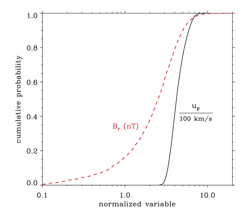
Figure 15.— Cumulative probability distributions extracted from OMNI data at 1 AU, where the abscissa corresponds to either $B_{r}$ in units of nT (red dashed curve) or $u_{p}$ in units of 100 km s^-1 (solid black curve).

In the ecliptic-plane OMNI data, the mass flux $\dot{M}$ did not appear to be strongly correlated with any other parameters. However, it does vary by about an order of magnitude between values of $7\times 10^{-15}$ and $6\times 10^{-14}$ $M_{\odot}$ yr^-1. Thus, we assumed a constant probability distribution in $\log\dot{M}$ and sampled it with a pseudorandom number uniformly distributed between $-14.15$ and $-13.22$. In combination with the randomly selected value of $u_{1{\rm AU}}$, Equation (81) provides a realistic distribution of densities at 1 AU. Initially, we experimented with randomly choosing the lower boundary conditions on $T_{p\parallel}$ and $T_{p\perp}$ from a distribution of likely coronal temperatures, but the results were similar to what we found with the standard boundary condition described above ($T_{p\parallel}=T_{p\perp}=T_{e}$).

It should be emphasized that our Monte Carlo procedure for selecting solar wind conditions is only a simplistic first attempt to “canvass” the full plasma parameter space. Our cumulative probability distributions did not explicitly exclude OMNI data taken during periods when interplanetary coronal mass ejections (ICMEs) were detected at 1 AU. Also, we did not consider the effects of stream–stream interactions in the ecliptic plane, which can produce plasma properties at 1 AU distinct from those that would otherwise be found in completely isolated flux tubes (see, e.g., Burlaga et al., 1983; Miyake et al., 1988; Riley & Lionello, 2011; Cranmer et al., 2013). Future attempts to compute more accurate heliospheric statistics will have to take both of these effects into account.

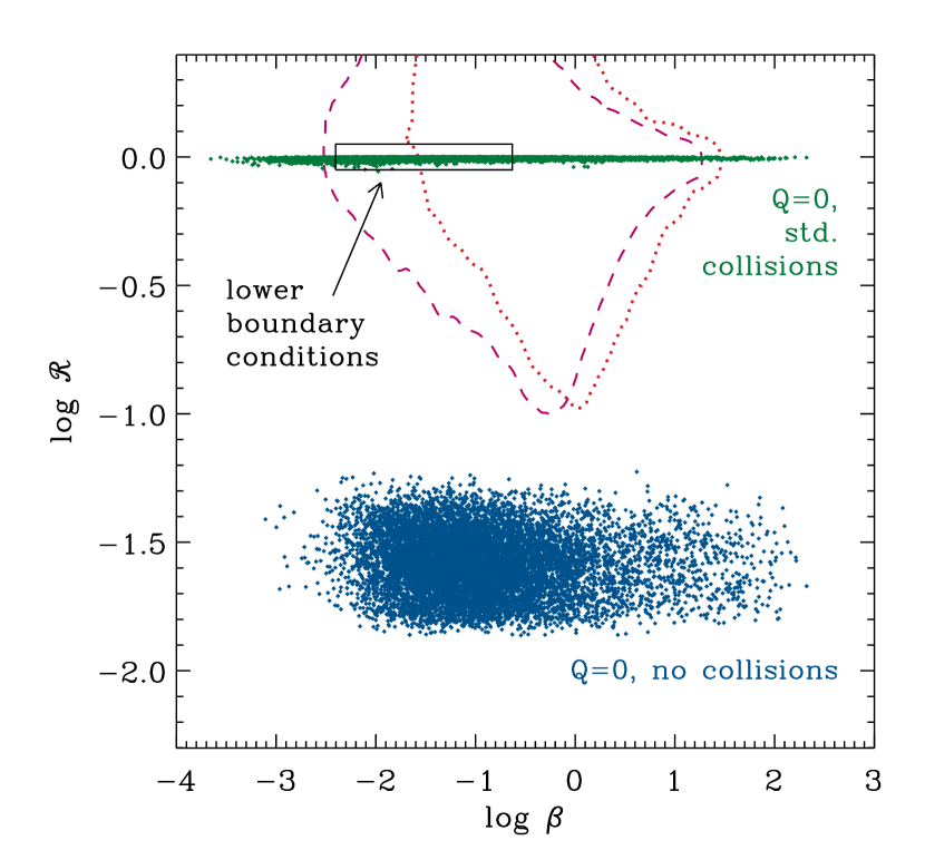
Figure 16.— Distributions of proton parameters at 1 AU in models with no heating and randomly varied $u_{1{\rm AU}}$, $B_{r,1{\rm AU}}$, and $\dot{M}$. Models with standard Coulomb collisions (green points) and without collisions (blue points) are compared to the range of initial values of $\beta$ (black box) and Wind data boundaries at 1 AU (red and magenta curves).

Prior to varying the heating rate parameters, we first show results of varying $u_{1{\rm AU}}$, $B_{r,1{\rm AU}}$, and $\dot{M}$ while fixing $Q_{1}=Q_{2}=0$. For this set of “no-heating” models, the firehose instability threshold of Equation (82) was not used. Figure 16 shows the conditions at 1 AU for $10^{4}$ random models with Coulomb collisions, and $10^{4}$ models without collisions. The same green/blue color scheme from Figure 13 is used in Figure 16. For both sets of models, the random variations in density and magnetic field strength gave rise to a distribution of lower boundary conditions on $\beta$. Most of the $\beta$ values at $r=2\,R_{\odot}$ fell between 0.004 and 0.23, which were the 5% and 95% percentile values of the distribution, respectively. The heliospheric evolution from 2 $R_{\odot}$ to 1 AU gave rise to ranges in $\beta$ that are reasonably close to what is observed, despite the fact that the distributions of ${\cal R}$ values were clearly unrealistic.

Next, Figure 17(a) shows the results of $10^{4}$ trials in which $u_{1{\rm AU}}$, $B_{r,1{\rm AU}}$, and $\dot{M}$ were varied randomly and the heating parameters were fixed at values discussed above for the strongly heated fast wind: $Q_{1}=1.596\times 10^{-6}$ erg s^-1 cm^-3, $\psi_{1}=4.150$, and $Q_{2}=1.660\times 10^{-6}$ erg s^-1 cm^-3. The symbol color is proportional to the resulting value of $T_{p}$ at 1 AU, similar to Figure 2 of Maruca et al. (2011). Unlike the more idealized sets of points shown in Figure 14, in this case the random variation of background wind conditions produces a significant “filled-in” region of the ($\beta$,${\cal R}$) diagram at 1 AU. However, only the right-hand side of the diagram is populated by the models (i.e., mainly $\beta\gtrsim 0.3$), since the fast-wind values of $Q_{1}$ and $Q_{2}$ represent rather strong rates of heating. It appears that only weaker heating rates will allow the left-hand side of the diagram to become filled in. The occupied part of parameter space in Figure 17(a) also resembles plots of measurements restricted to the fast wind, such as Figure 2 of Hellinger et al. (2006).

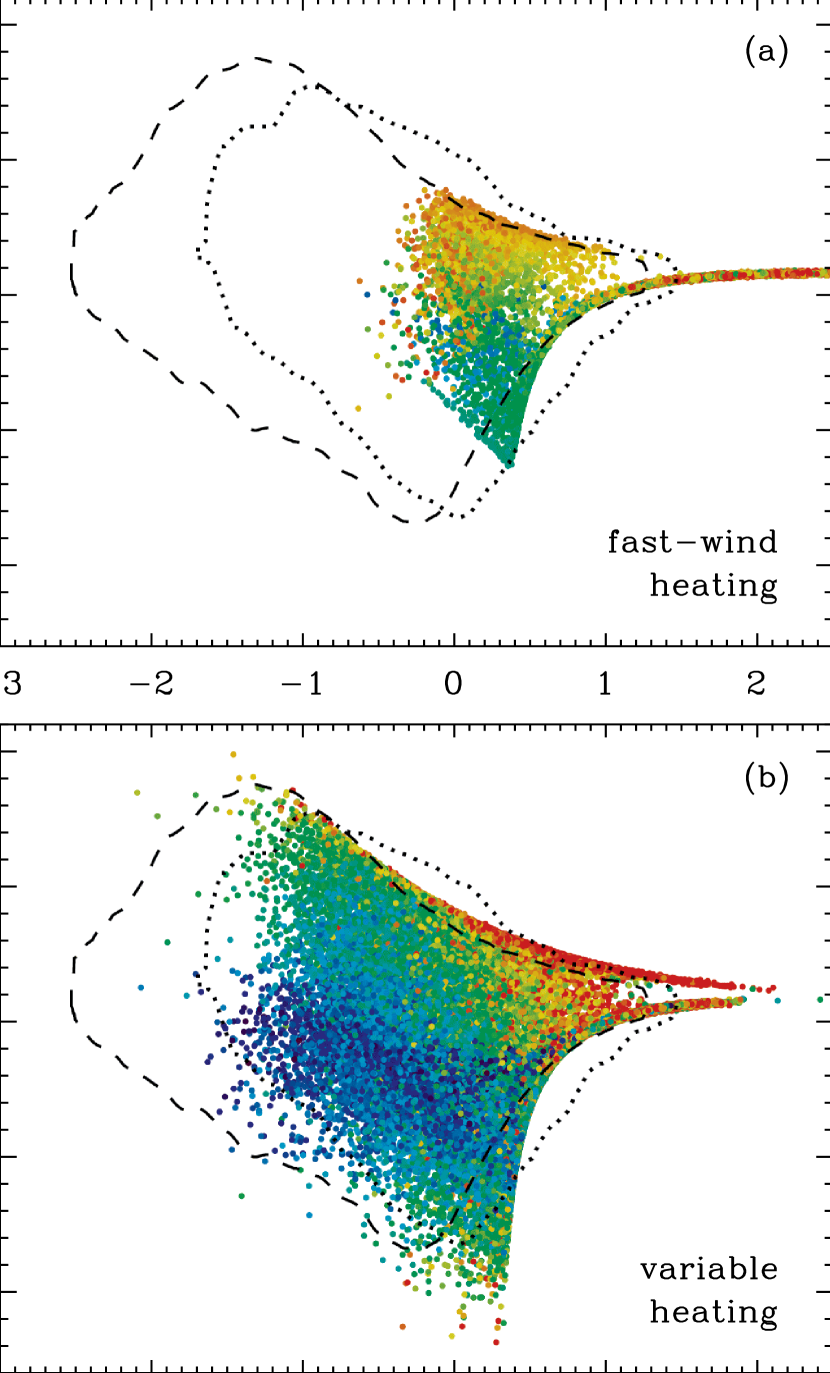
Figure 17.— Symbols show model results at 1 AU in the beta–anisotropy plane for random variations of solar wind parameters, with color corresponding to $T_{p}$ at 1 AU (see color bar). In both panels, the Wind data boundaries at 1 AU are shown with black dotted and dashed curves. Models were computed for (a) $Q_{p}$ fixed at the strongly heated fast-wind values from Section 6.2, and (b) randomly selected $Q_{p}$ parameters (see text).

Figure 17(b) shows the result of a full Monte Carlo simulation that involved varying all six parameters of the model. In addition to randomly choosing $u_{1{\rm AU}}$, $B_{r,1{\rm AU}}$, and $\dot{M}$, the proton heating rates were sampled from random distributions as well. $Q_{1}$ and $Q_{2}$ were each sampled uniformly on a logarithmic scale between $10^{-8}$ and $10^{-5}$ erg s^-1 cm^-3, and the value of $Q_{\rm cyc}$ at 1 AU was sampled uniformly between $10^{-17}$ and $10^{-14}$ erg s^-1 cm^-3. This produced a distribution in $\psi_{1}$ exponents that ranged between 2.57 and 5.14, and had a mean value of 3.85. Vertical bars in Figure 10 illustrate the ranges of variation of the heating rates at $r=2\,R_{\odot}$ and 1 AU. Even though the heating rates are varied over three orders of magnitude, these ranges never stray too far from existing expectations from other models and observations.

The full Monte Carlo model was run for 95,000 random trials. However, we found that roughly a third of these trials ended up with somewhat unrealistic conditions at 1 AU. Thus, Figure 17(b) shows only approximately 60,000 of them. Unrealistic models were excluded based on two criteria:

1. The largest collisional ages at 1 AU were found to correspond to models with unusually weak heating. Their heliospheric trajectories resembled the green dotted curves of Figure 13. Thus, we eliminated roughly 20,000 models that exhibited $A_{p}>2$ at 1 AU. Maruca et al. (2012) also made a similar collisional age cut to the Wind data in order to better isolate cases of collisionless wave-particle interaction. For the eliminated models, the mean value of $T_{p}$ at 1 AU was only 7,400 K, which is significantly smaller than the minimum proton temperature of $\sim$12,000 K seen in the OMNI data.

2. Even though the heating rates were not assumed to scale with the radial magnetic field strength, we do expect the solar wind to exhibit some kind of magnetic correlation (see, e.g., Pinto et al., 2009; Cranmer, 2009; Wang, 2010; Woolsey & Cranmer, 2014). Thus, it was not surprising to see that when the largest values of $Q_{2}$ were paired with the smallest values of $B_{r}$, the proton heating at 1 AU was unusually strong. This effect can be parameterized by computing the rate (i.e., inverse timescale) $\nu_{\rm B}=Q_{\rm iso}/U_{\rm B}$ at 1 AU, where $U_{\rm B}=B_{r}^{2}/8\pi$ is the magnetic energy density. Let us also define a normalizing value of $\nu_{\rm B}$ that corresponds to the strongly heated fast-wind model of Section 6.2; this value is given by $\nu_{{\rm B}\ast}=1.48\times 10^{-6}$ s^-1. The full grid of 90,000 models contained cases with $\nu_{\rm B}/\nu_{{\rm B}\ast}$ ranging over six orders of magnitude between $10^{-3}$ and $10^{+3}$. We eliminated roughly 15,000 models that exhibited $\nu_{\rm B}/\nu_{{\rm B}\ast}>5$. For that subsample, the mean values of $T_{p}$ and $\beta$ at 1 AU were 1.6 MK and 950, which are well above the maximum values from OMNI of $\sim$0.4 MK and $\sim$30, respectively.

Applying the above criteria gives rise to the $\sim$60,000 models shown in Figure 17(b). The area of occupied space in the beta–anisotropy plane agrees well with observations at 1 AU. Also, the correlation between $T_{p}$ (shown with symbol color) and location in the diagram is similar to that in the Wind data of Maruca et al. (2011). The left edges of the occupied region correspond to the lowest values of $\nu_{\rm B}$ at 1 AU. For those models, there is not enough heating “per unit field strength” to drive the wind to high $\beta$. Whether a weakly heated model winds up on the upper or lower left edge depends on the extent to which the heating is mostly isotropic or mostly cyclotron. At the left edge (i.e., for $\beta<0.1$), we found that the anisotropy ratio ${\cal R}_{\rm left}$ is strongly correlated with the heating ratio $Q_{\rm cyc}/Q_{\rm iso}$ at 1 AU, and

$${\cal R}_{\rm left}\,\approx\,0.15\sqrt{\left(\frac{Q_{\rm cyc}}{Q_{\rm iso}}\right)_{1\,{\rm AU}}}\,\,.$$ (83)

Thus, if this model captures the real physics of the solar wind, it requires there to be a broad range of partition fractions between the two types of heating. This range must also extend up to $Q_{\rm cyc}/Q_{\rm iso}\gtrsim 100$ in order to produce the upper-left edge of the diagram.

Figure 18 illustrates how the Monte Carlo models behave in terms of their Coulomb collisional coupling and relative alpha–proton drift. Here, we applied only the second of the two above criteria (i.e., eliminating models with $\nu_{\rm B}/\nu_{{\rm B}\ast}>5$) and we show the full range of collisional ages. The inverse temperature dependence in the collision rate is evident in that $A_{p}\propto T_{p}^{-3/2}$ (see also Hellinger & Trávníček, 2014). It is clear that the models experiencing the most frequent collisions are driven toward the lowest values of $\delta_{\alpha p}$ at 1 AU, and toward ${\cal R}\approx 1$. However, the least collisional models (i.e., $A_{p}\lesssim 10^{-4}$) also seem to be driven toward isotropy. These models have large values of $\beta$ at 1 AU and thus are constrained in ${\cal R}$ because of the cyclotron and firehose instability boundaries.

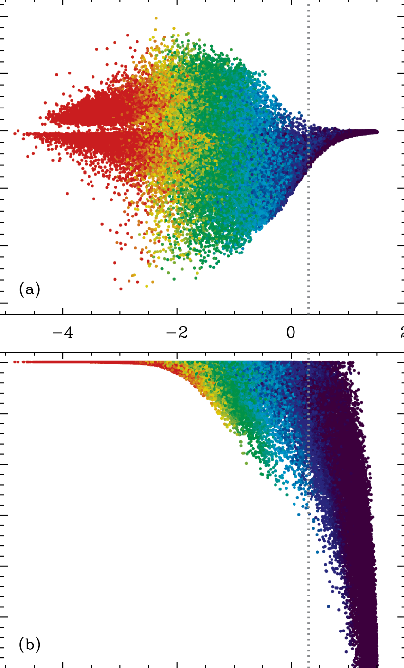
Figure 18.— Dependence of: (a) anisotropy ratio ${\cal R}$, (b) alpha–proton drift parameter $\delta_{\alpha p}$ on the collisional age $A_{p}$. Symbol colors are proportional to $T_{p}$ at 1 AU (see color bar). The gray dotted line illustrates the cutoff at $A_{p}=2$ applied to models shown Figure 17. Note that many of the “coldest” models to the right of the cutoff have $\log T_{p}$ that extends down to $\sim$3.5, but the color scale saturates at $\log T_{p}=4$.

7. Conclusions and Discussion

The goal of this paper was to begin exploring the detailed kinetic consequences of an assumed population of ion cyclotron resonant waves on the large-scale evolution of the solar wind. We found that the full range of kinetic properties of protons seen at 1 AU is generally reproducible with a stochastic ensemble of both background wind parameters and cyclotron heating rates. Other recent simulations (Seough et al., 2013; Servidio et al., 2014) have come to similar conclusions, but their random spreads of parameter choices were not so clearly connected to the actual “histories” of the modeled solar wind parcels. We also found that a broad range of relative contributions of ion cyclotron heating to the total heating rate (i.e., a broad range of $Q_{\rm cyc}/Q_{\rm iso}$ ratios) may be important to reproducing the low-$\beta$ part of observed parameter space.

In the process of building models of proton VDF transport from the corona to 1 AU, some additional key physical properties of ion cyclotron resonance were revealed. For example,

1. In Section 3.1, a two-term asymptotic expansion of the plasma dispersion function was used to derive a new analytic “warm plasma” dispersion relation that simultaneously deals with both ion cyclotron resonance and the firehose-unstable regime. This dispersion relation (see Equation (18) and Figure 1(b)) also reproduces much of the $\beta$ and anisotropy dependence found in numerical Alfvén-wave solutions of the full Vlasov-Maxwell dispersion relation.

2. In Section 3.3, we found analytic expressions for a modified plasma dispersion function consistent with a simple form of a non-Maxwellian “resonant shell” proton VDF. Although the resulting dispersion relation was found to be equivalent to the two-term expansion discussed above, this derivation showed that some results coming from bi-Maxwellian theory may still be applicable to other types of kinetic distributions.

3. Section 4.2 described a generalization of quasilinear theory that replaces the Dirac delta function associated with wave-particle resonance with a more realistic Lorentzian function that depends on the damping rate $\gamma$. This expression leads to nonzero VDF diffusion coefficients in regions of velocity space that are classically nonresonant (e.g., $v_{\parallel}>0$ for the resonance between protons and forward-propagating ion cyclotron waves).

4. The numerical VDF diffusion models of Cranmer (2001) were extended to protons in the presence of both forward- and backward-propagating Alfvén waves. The early-time evolution of proton temperature moments was found to be nearly identical to equivalent bi-Maxwellian calculations. Also, it appeared that the late-time evolution into non-Maxwellian shell-type VDFs exhibits cross-shell perpendicular diffusion (see, e.g., Isenberg, 2001) even for purely forward-propagating waves.

5. In Section 4.3, we solved for the locations of marginal stability curves (defined by a vanishing time derivative of the proton anisotropy ratio) in the beta–anisotropy plane for several different dispersion relations. Figures 4(b) and 9 displayed a surprising diversity of curve shapes. This indicates that any conclusions made about the ion cyclotron instability boundaries may be extremely sensitive to assumptions made about the wave dispersion and particle VDFs.

6. Section 5 outlined a damped cascade model that describes how drifting alpha particles may intercept ion cyclotron waves prior to them becoming resonant with protons. Figure 12 shows how this model appears able to reproduce an empirical dividing line in ($\beta$, $\delta_{\alpha p}$) space seen in Wind data (Kasper et al., 2013).

Despite the new insights gained from the exploratory modeling described above, it did not completely reproduce all observational constraints. At any rate, it points the way to improved methods of simulating the radial evolution of a realistic ensemble of solar wind states. Other proposed explanations for preferential proton heating in the heliosphere—such as stochastic KAW heating (Chandran, 2010; Chandran et al., 2011, 2013; Bourouaine & Chandran, 2013)—can be straightforwardly plugged into the same kind of transport model as the one described in Section 6.

In addition to the need for testing other physical processes, it is also clear that the existing models of ion cyclotron resonance need to be improved in several important ways. This paper relied heavily on the bi-Maxwellian assumption. One of our goals was in fact to explore in detail how bi-Maxwellians can be useful tools for understanding the kinetic physics of the solar wind. However, it is well-known that measured VDFs often exhibit marked departures from this simple parameterization. Other kinetic simulation approaches (Isenberg & Vasquez, 2011; Galinsky & Shevchenko, 2013; Araneda et al., 2013; Maneva et al., 2014; Servidio et al., 2014) are helping to make clear how specific departures from the bi-Maxwellian model affect the conclusions made about the large-scale energy balance of the heliosphere.

The models described in this paper were also limited to purely parallel-propagating Alfvén waves. However, the solar wind fluctuation spectrum is known to exhibit a broad range of propagation angles. There have been several studies of the radial evolution of this angular distribution (Bavassano et al., 1982; Horbury et al., 1995; Neugebauer, 2004; He et al., 2013). Although there is still no agreement on the overall sense of the evolution—i.e., is it becoming more parallel or more perpendicular with increasing distance?—it is evident that there must be wave power at all values of $\theta$. Obliquely propagating Alfvén/ion-cyclotron waves have been studied extensively in a solar wind context (see, e.g., Li & Habbal, 2001; Harmon & Coles, 2005; Chandran et al., 2010; Li & Lu, 2010; He et al., 2012), and some properties of the particle heating are different from the parallel-propagating case.

Understanding the proton thermodynamics might also depend on including couplings between Alfvén waves and other compressive MHD modes (see Cranmer & van Ballegooijen, 2012; Maneva et al., 2014, and references therein). One possibly important example, not studied in this paper, is the mirror-mode wave. It has been claimed that the upper-right boundary in the beta–anisotropy diagram is better described by the mirror instability than by the cyclotron instability (e.g., Hellinger et al., 2006; Bale et al., 2009; Maruca et al., 2012). Mirror-mode waves have been detected sporadically in the solar wind (Russell et al., 2009), and it is possible that the well-known pressure-balanced structures (PBSs) may be caused by them (Yao et al., 2013). It is interesting to note that Leubner (1981) modeled solar wind ion VDFs using a skewed non-Maxwellian function meant to be consistent with a nonzero heat flux, and found that the mirror instability completely disappears, leaving only the ion cyclotron instability for ${\cal R}>1$.

Lastly, the properties of the alpha particles should be modeled simultaneously with the protons, and with a comparable degree of physical realism (see, e.g., Bourouaine et al., 2013; Chandran et al., 2013; Moya et al., 2014). At the very least, the sensitivity of the results in Sections 5–6 to our assumption that $T_{\alpha}/T_{p}=4$ needs to be explored. It would also be beneficial for models to make predictions of the detailed plasma properties of protons and alpha particles at a range of distances that extends down to $\sim$9 $R_{\odot}$, the latter being the inner boundary of future exploration by Solar Probe Plus (Fox et al., 2013).

References

- Abraham-Shrauner & Feldman (1977) Abraham-Shrauner, B., & Feldman, W. C. 1977, J. Geophys. Res., 82, 618
- Araneda et al. (2013) Araneda, J. A., Astudillo, H., & Marsch, E. 2013, Space Sci. Rev., 172, 361
- Artemyev et al. (2014) Artemyev, A. V., Zimbardo, G., Ukhorskiy, A. Y., et al. 2014, A&A, 562, A58
- Arunasalam (1976) Arunasalam, V. 1976, Phys. Rev. Lett., 37, 746
- Axford & McKenzie (1992) Axford, W. I., & McKenzie, J. F. 1992, in Solar Wind Seven, ed. E. Marsch & R. Schwenn (New York: Pergamon), 1
- Bale et al. (2009) Bale, S. D., Kasper, J. C., Howes, G. G., et al. 2009, Phys. Rev. Lett., 103, 211101
- Barakat & Schunk (1982) Barakat, A. R., & Schunk, R. W. 1982, Plasma Phys., 24, 389
- Barnes (1966) Barnes, A. 1966, Phys. Fluids, 9, 1483
- Bavassano et al. (1982) Bavassano, B., Dobrowolny, M., Fanfoni, G., et al. 1982, Sol. Phys., 78, 373
- Benz (1993) Benz, A. O. 1993, Plasma Astrophysics: Kinetic Processes in Solar and Stellar Coronae (Dordrecht: Kluwer)
- Berger et al. (2011) Berger, L., Wimmer-Schweingruber, R. F., & Gloeckler, G. 2011, Phys. Rev. Lett., 106, 151103
- Bieber et al. (1996) Bieber, J. W., Wanner, W., & Matthaeus, W. H. 1996, J. Geophys. Res., 101, 2511
- Bingert & Peter (2011) Bingert, S., & Peter, H. 2011, A&A, 530, A112
- Boldyrev (2006) Boldyrev, S. 2006, Phys. Rev. Lett., 96, 115002
- Bourouaine & Chandran (2013) Bourouaine, S., & Chandran, B. D. G. 2013, ApJ, 774, 96
- Bourouaine et al. (2011) Bourouaine, S., Marsch, E., & Neubauer, F. M. 2011, A&A, 536, A39
- Bourouaine et al. (2013) Bourouaine, S., Verscharen, D., Chandran, B. D. G., et al. 2013, ApJ, 777, L3
- Brambilla (1998) Brambilla, M. 1998, Kinetic Theory of Plasma Waves: Homogeneous Plasmas (Oxford: Clarendon)
- Bruno & Carbone (2013) Bruno, R., & Carbone, V. 2013, Living Rev. Solar Phys., 10, 2
- Burlaga et al. (1983) Burlaga, L. F., Schwenn, R., & Rosenbauer, H. 1983, Geophys. Res. Lett., 10, 413
- Chandran (2005) Chandran, B. D. G. 2005, Phys. Rev. Lett., 95, 265004
- Chandran (2008) Chandran, B. D. G. 2008, Phys. Rev. Lett., 101, 235004
- Chandran (2010) Chandran, B. D. G. 2010, ApJ, 720, 548
- Chandran et al. (2011) Chandran, B. D. G., Dennis, T. J., Quataert, E., & Bale, S. D. 2011, ApJ, 743, 197
- Chandran et al. (2010) Chandran, B. D. G., Pongkitiwanichakul, P., Isenberg, P. A., et al. 2010, ApJ, 722, 710
- Chandran et al. (2013) Chandran, B. D. G., Verscharen, D., Quataert, E., et al. 2013, ApJ, 776, 45
- Chen et al. (2013) Chen, C. H. K., Boldyrev, S., Xia, Q., et al. 2013, Phys. Rev. Lett., 110, 225002
- Chen et al. (2010) Chen, C. H. K., Horbury, T. S., Schekochihin, A. A., et al. 2010, Phys. Rev. Lett., 104, 25502
- Chew et al. (1956) Chew, G. F., Goldberger, M. L., & Low, F. E. 1956, Proc. Roy. Soc. London, A, 236, 112
- Cranmer (2000) Cranmer, S. R. 2000, ApJ, 532, 1197
- Cranmer (2001) Cranmer, S. R. 2001, J. Geophys. Res., 106, 24937
- Cranmer (2009) Cranmer, S. R. 2009, Living Rev. Solar Phys., 6, 3
- Cranmer et al. (1999) Cranmer, S. R., Field, G. B., & Kohl, J. L. 1999, ApJ, 518, 937
- Cranmer et al. (2009) Cranmer, S. R., Matthaeus, W. H., Breech, B. A., et al. 2009, ApJ, 702, 1604
- Cranmer & van Ballegooijen (2003) Cranmer, S. R., & van Ballegooijen, A. A. 2003, ApJ, 594, 573
- Cranmer & van Ballegooijen (2012) Cranmer, S. R., & van Ballegooijen, A. A. 2012, ApJ, 754, 92
- Cranmer et al. (2007) Cranmer, S. R., van Ballegooijen, A. A., & Edgar, R. J. 2007, ApJS, 171, 520
- Cranmer et al. (2013) Cranmer, S. R., van Ballegooijen, A. A., & Woolsey, L. N. 2013, ApJ, 767, 125
- Cuperman et al. (1975) Cuperman, S., Gomberoff, L., & Sternlieb, A. 1975, J. Plasma Phys., 13, 259
- Dasso et al. (2005) Dasso, S., Milano, L. J., Matthaeus, W. H., et al. 2005, ApJ, 635, L181
- Davidson (1983) Davidson, R. C. 1983, in Basic Plasma Physics I, ed. A. A. Galeev & R. N. Sudan (Amsterdam: North Holland), 519
- Denton et al. (1994) Denton, R. E., Anderson, B. J., Gary, S. P., & Fuselier, S. A. 1994, J. Geophys. Res., 99, 11225
- Dmitruk et al. (2002) Dmitruk, P., Matthaeus, W. H., Milano, L. J., et al. 2002, ApJ, 575, 571
- Dmitruk et al. (2004) Dmitruk, P., Matthaeus, W. H., & Seenu, N. 2004, ApJ, 617, 667
- Dong & Singh (2013) Dong,C., & Singh, N. 2013, Phys. Plasmas, 20, 012121
- Drake et al. (2009) Drake, J. F., Swisdak, M., Phan, T. D., et al. 2009, J. Geophys. Res., 114, A05111
- Dusenbery & Hollweg (1981) Dusenbery, P. B., & Hollweg, J. V. 1981, J. Geophys. Res., 86, 153
- Fox et al. (2013) Fox, N. J., Bale, S. D., Decker, R. B., et al. 2013, Eos Trans. AGU, Fall Meet. Suppl., abstract SM53A-2207
- Fried & Conte (1961) Fried, B. D., & Conte, S. D. 1961, The Plasma Dispersion Function (New York: Academic)
- Galeev & Sagdeev (1983) Galeev, A. A., & Sagdeev, R. Z. 1983, in Basic Plasma Physics I, ed. A. A. Galeev & R. N. Sudan (Amsterdam: North Holland), 683
- Galinsky & Shevchenko (2000) Galinsky, V. L., & Shevchenko, V. I. 2000, Phys. Rev. Lett., 85, 90
- Galinsky & Shevchenko (2013) Galinsky, V. L., & Shevchenko, V. I. 2013, Phys. Rev. Lett., 111, 015004
- Gary (1993) Gary, S. P. 1993, Theory of Space Plasma Microinstabilities (Cambridge: Cambridge Univ. Press)
- Gary & Borovsky (2004) Gary, S. P., & Borovsky, J. E. 2004, J. Geophys. Res., 109, A06105
- Gary & Borovsky (2008) Gary, S. P., & Borovsky, J. E. 2008, J. Geophys. Res., 113, A12104
- Gary et al. (1998) Gary, S. P., Li, H., O’Rourke, S., et al. 1998, J. Geophys. Res., 103, 14567
- Gary & Saito (2003) Gary, S. P., & Saito, S. 2003, J. Geophys. Res., 108, 1194
- Gary et al. (2001) Gary, S. P., Skoug, R. M., Steinberg, J. T., et al. 2001, Geophys. Res. Lett., 28, 2759
- Gary et al. (2005) Gary, S. P., Smith, C. W., & Skoug, R. M. 2005, J. Geophys. Res., 110, A07108
- Goldreich & Sridhar (1995) Goldreich, P., & Sridhar, S. 1995, ApJ, 438, 763
- Gomberoff & Elgueta (1991) Gomberoff, L., & Elgueta, R. 1991, J. Geophys. Res., 96, 9801
- Gomberoff et al. (1994) Gomberoff, L., Gratton, F., & Gnavi, G. 1994, J. Geophys. Res., 99, 14717
- Grappin et al. (2013) Grappin, R., Müller, W.-C., Verdini, A., et al. 2013, preprint, arXiv:1312.3459
- Griffel & Davis (1969) Griffel, D. H., & Davis, L. 1969, Planet. Space Sci., 17, 1009
- Harmon & Coles (2005) Harmon, J. K., & Coles, W. A. 2005, J. Geophys. Res., 110, A03101
- Hartle & Sturrock (1968) Hartle, R. E., & Sturrock, P. A. 1968, ApJ, 151, 1155
- Haynes et al. (2014) Haynes, C. T., Burgess, D., & Camporeale, E. 2014, ApJ, 783, 38
- He et al. (2011) He, J.-S., Marsch, E., Tu, C.-Y., et al. 2011, ApJ, 731, 85
- He et al. (2012) He, J.-S., Tu, C.-Y., Marsch, E., et al. 2012, ApJ, 745, L8
- He et al. (2013) He, J.-S., Tu, C.-Y., Marsch, E., et al. 2013, ApJ, 773, 72
- Hefti et al. (1998) Hefti, S., Grünwaldt, H., Ipavich, F. M., et al. 1998, J. Geophys. Res., 103, 29697
- Hellinger & Trávníček (2009) Hellinger, P., & Trávníček, P. 2009, Phys. Plasmas, 16, 054501
- Hellinger & Trávníček (2014) Hellinger, P., & Trávníček, P. 2014, ApJ, 784, L15
- Hellinger et al. (2006) Hellinger, P., Trávníček, P., Kasper, J. C., et al. 2006, Geophys. Res. Lett., 33, L09101
- Hellinger et al. (2013) Hellinger, P., Trávníček, P., Štverák, Š., et al. 2013, J. Geophys. Res., 118, 1351
- Hernández et al. (1987) Hernández, R., Livi, S., & Marsch, E. 1987, J. Geophys. Res., 92, 7723
- Hollweg (1971) Hollweg, J. V. 1971, J. Geophys. Res., 76, 7491
- Hollweg (1999) Hollweg, J. V. 1999, J. Geophys. Res., 104, 24781
- Hollweg (2000) Hollweg, J. V. 2000, J. Geophys. Res., 105, 7573
- Hollweg (2008) Hollweg, J. V. 2008, J. Astrophys. Astron., 29, 217
- Hollweg & Isenberg (2002) Hollweg, J. V., & Isenberg, P. A. 2002, J. Geophys. Res., 107, 1147
- Hollweg & Turner (1978) Hollweg, J. V., & Turner, J. M. 1978, J. Geophys. Res., 83, 97
- Horbury et al. (1995) Horbury, T. S., Balogh, A., Forsyth, R. J., et al. 1995, Geophys. Res. Lett., 22, 3405
- Horbury et al. (2008) Horbury, T. S., Forman, M., & Oughton, S. 2008, Phys. Rev. Lett., 101, 175005
- Howes et al. (2006) Howes, G. G., Cowley, S. C., Dorland, W., et al. 2006, ApJ, 651, 590
- Howes et al. (2008) Howes, G. G., Cowley, S. C., Dorland, W., et al. 2008, J. Geophys. Res., 113, A05103
- Howes & Nielson (2013) Howes, G. G., & Nielson, K. D. 2013, Phys. Plasmas, 20, 072302
- Iroshnikov (1963) Iroshnikov, P. S. 1963, AZh, 40, 742
- Isenberg (1984a) Isenberg, P. A. 1984a, J. Geophys. Res., 89, 2133
- Isenberg (1984b) Isenberg, P. A. 1984b, J. Geophys. Res., 89, 6613
- Isenberg (2001) Isenberg, P. A. 2001, Space Sci. Rev., 95, 119
- Isenberg (2012) Isenberg, P. A. 2012, Phys. Plasmas, 19, 032116
- Isenberg & Hollweg (1983) Isenberg, P. A., & Hollweg, J. V. 1983, J. Geophys. Res., 88, 3923
- Isenberg et al. (2000) Isenberg, P. A., Lee, M. A., & Hollweg, J. V. 2000, Solar Phys., 193, 247
- Isenberg et al. (2013) Isenberg, P. A., Maruca, B. A., & Kasper, J. C. 2013, ApJ, 773, 164
- Isenberg & Vasquez (2007) Isenberg, P. A., & Vasquez, B. J. 2007, ApJ, 668, 546
- Isenberg & Vasquez (2011) Isenberg, P. A., & Vasquez, B. J. 2011, ApJ, 731, 88
- Jess et al. (2009) Jess, D. B., Mathioudakis, M., Erdélyi, R., et al. 2009, Science, 323, 1582
- Jian et al. (2009) Jian, L. K., Russell, C. T., Luhmann, J. G., et al. 2009, ApJ, 701, L105
- Jian et al. (2010) Jian, L. K., Russell, C. T., Luhmann, J. G., et al. 2010, J. Geophys. Res., 115, A12115
- Jiang et al. (2009) Jiang, Y. W., Liu, S., & Petrosian, V. 2009, ApJ, 698, 163
- Johnson & Cheng (2001) Johnson, J. R., & Cheng, C. Z. 2001, Geophys. Res. Lett., 28, 4421
- Karimabadi et al. (2013) Karimabadi, H., Roytershteyn, V., Wan, M., et al. 2013, Phys. Plasmas, 20, 012303
- Kasper et al. (2008) Kasper, J. C., Lazarus, A. J., & Gary, S. P. 2008, Phys. Rev. Lett., 101, 261103
- Kasper et al. (2013) Kasper, J. C., Maruca, B. A., Stevens, M. L., & Zaslavsky, A. 2013, Phys. Rev. Lett., 110, 091102
- Kennel & Engelmann (1966) Kennel, C. F., & Engelmann, F. 1966, Phys. Fluids, 9, 2377
- King & Papitashvili (2005) King, J. H., & Papitashvili, N. E. 2005, J. Geophys. Res., 110, A02104
- Klimchuk (2006) Klimchuk, J. A. 2006, Sol. Phys., 234, 41
- Kohl et al. (1997) Kohl, J. L., Noci, G., Antonucci, E., et al. 1997, Sol. Phys., 175, 613
- Kohl et al. (2006) Kohl, J. L., Noci, G., Cranmer, S. R., & Raymond, J. C. 2006, A&A Rev., 13, 31
- Kraichnan (1965) Kraichnan, R. H. 1965, Phys. Fluids, 8, 1385
- Leamon et al. (1999) Leamon, R. J., Smith, C. W., Ness, N. F., & Wong, H. K. 1999, J. Geophys. Res., 104, 22331
- Lee (1971) Lee, M. A. 1971, Plasma Phys., 13, 1079
- Leer & Axford (1972) Leer, E., & Axford, W. I. 1972, Sol. Phys., 23, 238
- Lehe et al. (2009) Lehe, R., Parrish, I. J., & Quataert, E. 2009, ApJ, 707, 404
- Leubner (1981) Leubner, M. P. 1981, J. Geophys. Res., 86, 7787
- Li et al. (2001) Li, H., Gary, S. P., & Stawicki, O. 2001, Geophys. Res. Lett., 28, 1347
- Li (1999) Li, X. 1999, J. Geophys. Res., 104, 19773
- Li & Habbal (2001) Li, X., & Habbal, S. R. 2001, J. Geophys. Res., 106, 10669
- Li & Lu (2010) Li, X., & Lu, Q. M. 2010, J. Geophys. Res., 115, A08105
- Liewer et al. (2001) Liewer, P. C., Velli, M., & Goldstein, B. E. 2001, J. Geophys. Res., 106, 29261
- Lionello et al. (2014) Lionello, R., Velli, M., Downs, C., et al. 2014, ApJ, 784, 120
- Livi & Marsch (1987) Livi, S., & Marsch, E. 1987, J. Geophys. Res., 92, 7255
- Lynn et al. (2012) Lynn, J. W., Parrish, I. J., Quataert, E., et al. 2012, ApJ, 758, 78
- MacBride et al. (2008) MacBride, B. T., Smith, C. W., & Forman, M. A. 2008, ApJ, 679, 1644
- Maneva et al. (2014) Maneva, Y. G., Araneda, J. A., & Marsch, E. 2014, ApJ, 783, 139
- Maneva et al. (2013) Maneva, Y. G., Viñas, A., & Ofman, L. 2013, J. Geophys. Res., 118, 2842
- Markovskii (2001) Markovskii, S. A. 2001, ApJ, 557, 337
- Markovskii et al. (2009) Markovskii, S. A., Vasquez, B. J., & Hollweg, J. V. 2009, ApJ, 695, 1413
- Markovskii et al. (2006) Markovskii, S. A., Vasquez, B. J., Smith, C. W., et al. 2006, ApJ, 639, 1177
- Maron & Goldreich (2001) Maron, J., & Goldreich, P. 2001, ApJ, 554, 1175
- Marsch (2006) Marsch, E. 2006, Living Rev. Solar Phys., 3, 1
- Marsch (2012) Marsch, E. 2012, Space Sci. Rev., 172, 23
- Marsch et al. (1983) Marsch, E., Mühlhäuser, K.-H, Rosenbauer, H., et al. 1983, J. Geophys. Res., 88, 2982
- Marsch et al. (1982) Marsch, E., Mühlhäuser, K.-H, Schwenn, R., et al. 1982, J. Geophys. Res., 87, 52
- Marsch & Tu (2001a) Marsch, E., & Tu, C.-Y. 2001a, J. Geophys. Res., 106, 227
- Marsch & Tu (2001b) Marsch, E., & Tu, C.-Y. 2001b, J. Geophys. Res., 106, 8357
- Maruca et al. (2011) Maruca, B. A., Kasper, J. C., & Bale, S. D. 2011, Phys. Rev. Lett., 107, 201101
- Maruca et al. (2012) Maruca, B. A., Kasper, J. C., & Gary, S. P. 2012, ApJ, 748, 137
- Matsumoto & Suzuki (2014) Matsumoto, T., & Suzuki, T. K. 2014, MNRAS, 440, 971
- Matteini et al. (2012) Matteini, L., Hellinger, P., Landi, S., et al. 2012, Space Sci. Rev., 172, 373
- Matthaeus et al. (2003) Matthaeus, W. H., Dmitruk, P., Oughton, S., et al. 2003, in Solar Wind Ten, AIP Conf. Ser. 679, ed. M. Velli, R. Bruno, & F. Malara (Melville, NY: AIP), 427
- Matthaeus & Velli (2011) Matthaeus, W. H., & Velli, M. 2011, Space Sci. Rev., 160, 145
- Matthaeus et al. (1999) Matthaeus, W. H., Zank, G. P., Leamon, R. J., et al. 1999, Space Sci. Rev., 87, 269
- McIntosh et al. (2011) McIntosh, S. W., de Pontieu, B., Carlsson, M., et al. 2011, Nature, 475, 477
- Medvedev (2000) Medvedev, M. V. 2000, ApJ, 541, 811
- Melrose (1986) Melrose, D. B. 1986, Instabilities in Space and Laboratory Plasmas (Cambridge: Cambridge Univ. Press)
- Michno et al. (2014) Michno, M. J., Lazar, M., Yoon, P. H., et al. 2014, ApJ, 781, 49
- Mikhailenko et al. (2008) Mikhailenko, V. S., Mikhailenko, V. V., & Stepanov, K. N. 2008, Phys. Plasmas, 15, 092901
- Miyake et al. (1988) Miyake, W., Mukai, T., Terasawa, T., et al. 1988, Sol. Phys., 117, 171
- Montgomery & Tidman (1964) Montgomery, D. C., & Tidman, D. A. 1964, Plasma Kinetic Theory (New York: McGraw-Hill)
- Montgomery & Turner (1981) Montgomery, D., & Turner, L. 1981, Phys. Fluids, 24, 825
- Moya et al. (2014) Moya, P. S., Navarro, R., Viñas, A. F., et al. 2014, ApJ, 781, 76
- Nakayama (1999) Nakayama, K. 1999, ApJ, 523, 315
- Nariyuki et al. (2014) Nariyuki, T., Umeda, T., Suzuki, T. K., et al. 2014, Nonlin. Proc. Geophys., 21, 339
- Neugebauer (1982) Neugebauer, M. 1982, Space Sci. Rev., 33, 127
- Neugebauer (2004) Neugebauer, M. 2004, J. Geophys. Res., 109, A02101
- Ng & Bhattacharjee (1996) Ng, C. S., & Bhattacharjee, A. 1996, ApJ, 465, 845
- Ofman (2010) Ofman, L. 2010, Living Rev. Solar Phys., 7, 4
- Parashar et al. (2009) Parashar, T. N., Shay, M. A., Cassak, P. A., et al. 2009, Phys. Plasmas, 16, 032310
- Park & Miller (1988) Park, S. K., & Miller, K. W. 1988, Comm. ACM, 31, 1192
- Parnell & De Moortel (2012) Parnell, C. E., & De Moortel, I. 2012, Phil. Trans. Roy. Soc. A, 370, 3217
- Perez & Chandran (2013) Perez, J. C., & Chandran, B. D. G. 2013, ApJ, 776, 124
- Pinto et al. (2009) Pinto, R., Grappin, R., Wang, Y.-M., et al. 2009, A&A, 497, 537
- Podesta (2013) Podesta, J. J. 2013, Sol. Phys., 286, 529
- Podesta & Gary (2011) Podesta, J. J., & Gary, S. P. 2011, ApJ, 742, 41
- Riley & Lionello (2011) Riley, P., & Lionello, R. 2011, Sol. Phys., 270, 575
- Roberts et al. (2013) Roberts, O. W., Li, X., & Li, B. 2013, ApJ, 769, 58
- Rosin et al. (2011) Rosin, M. S., Schekochihin, A. A., Rincon, F., et al. 2011, MNRAS, 413, 7
- Rowlands et al. (1966) Rowlands, J., Shapiro, V. D., & Shevchenko, V. I. 1966, Soviet Phys. JETP, 23, 651
- Rudakov et al. (2012) Rudakov, L., Crabtree, C., Ganguli, G., et al. 2012, Phys. Plasmas, 19, 042704
- Russell et al. (2009) Russell, C. T., Blanco-Cano, X., Jian, L. K., et al. 2009, Geophys. Res. Lett., 36, L05106
- Sahraoui et al. (2010) Sahraoui, F., Goldstein, M. L., Belmont, G., et al. 2010, Phys. Rev. Lett., 105, 131101
- Salem et al. (2012) Salem, C. S., Howes, G. G., Sundkvist, D., et al. 2012, ApJ, 745, L9
- Sandbaek & Leer (1995) Sandbaek, O., & Leer, E. 1995, ApJ, 454, 486
- Schlickeiser & Skoda (2010) Schlickeiser, R., & Skoda, T. 2010, ApJ, 716, 1596
- Seough & Yoon (2009) Seough, J., & Yoon, P. H. 2009, Phys. Plasmas, 16, 092103
- Seough et al. (2013) Seough, J., Yoon, P. H., Kim, K.-H., & Lee, D.-H. 2013, Phys. Rev. Lett., 110, 071103
- Servidio et al. (2014) Servidio, S., Osman, K. T., Valentini, F., et al. 2014, ApJ, 781, L27
- Servidio et al. (2012) Servidio, S., Valentini, F., Califano, F., et al. 2012, Phys. Rev. Lett., 108, 045001
- Sharma et al. (2006) Sharma, P., Hammett, G. W., Quataert, E., et al. 2006, ApJ, 637, 952
- Shebalin et al. (1983) Shebalin, J. V., Matthaeus, W. H., & Montgomery, D. 1983, J. Plasma Phys., 29, 525
- Smith et al. (2012) Smith, C. W., Vasquez, B. J., & Hollweg, J. V. 2012, ApJ, 745, 8
- Stix (1992) Stix, T. H. 1992, The Theory of Plasma Waves (New York: McGraw-Hill)
- Strauss (1976) Strauss, H. R. 1976, Phys. Fluids, 19, 134
- Tsurutani et al. (1994) Tsurutani, B. T., Arballo, J. K., Mok, J., et al. 1994, Geophys. Res. Lett., 21, 633
- Tu & Marsch (1995) Tu, C.-Y., & Marsch, E. 1995, Space Sci. Rev., 73, 1
- Tu & Marsch (1997) Tu, C.-Y., & Marsch, E. 1997, Sol. Phys., 171, 363
- Tu et al. (2003) Tu, C.-Y., Wang, L.-H., & Marsch, E. 2003, J. Geophys. Res., 108, 1161
- Vasquez et al. (2007) Vasquez, B. J., Smith, C. W., Hamilton, K., et al. 2007, J. Geophys. Res., 112, A07101
- Verscharen et al. (2013) Verscharen, D., Bourouaine, S., Chandran, B. D. G., & Maruca, B. A. 2013, ApJ, 773, 8
- Voitenko & Goossens (2004) Voitenko, Y., & Goossens, M. 2004, ApJ, 605, L149
- Voitenko & Pierrard (2013) Voitenko, Y., & Pierrard, V. 2013, Sol. Phys., 288, 369
- Vranjes & Poedts (2008) Vranjes, J., & Poedts, S. 2008, A&A, 482, 653
- Wang (2010) Wang, Y.-M. 2010, ApJ, 715, L121
- Weber & Davis (1967) Weber, E. J., & Davis, L., Jr. 1967, ApJ, 148, 217
- Wilhelm et al. (2011) Wilhelm, K., Abbo, L., Auchère, F., et al. 2011, A&A Rev., 19, 35
- Woolsey & Cranmer (2014) Woolsey, L. N., & Cranmer, S. R. 2014, ApJ, 787, 160
- Xie et al. (2004) Xie, H., Ofman, L., & Viñas, A. 2004, J. Geophys. Res., 109, A08103
- Yao et al. (2013) Yao, S., He. J.-S., Tu, C.-Y., et al. 2013, ApJ, 776, 94
- Yoon et al. (2010) Yoon, P. H., Seough, J. J., Khim, K. K., et al. 2010, Phys. Plasmas, 17, 082111
- Zurbuchen (2007) Zurbuchen, T. H. 2007, ARA&A, 45, 297