Decision Algorithms for Fibonacci-Automatic Words, with Applications to Pattern Avoidance

Abstract

We implement a decision procedure for answering questions about a class of infinite words that might be called (for lack of a better name) “Fibonacci-automatic”. This class includes, for example, the famous Fibonacci word ${\bf f}=01001010\cdots$, the fixed point of the morphism $0\rightarrow 01$ and $1\rightarrow 0$. We then recover many results about the Fibonacci word from the literature (and improve some of them), such as assertions about the occurrences in $\bf f$ of squares, cubes, palindromes, and so forth. As an application of our method we prove a new result: there exists an aperiodic infinite binary word avoiding the pattern $xxx^{R}$. This is the first avoidability result concerning a nonuniform morphism proven purely mechanically.

1 Decidability

As is well-known, the logical theory $\operatorname{Th}({\mathbb{N}},+)$, sometimes called Presburger arithmetic, is decidable [62, 63]. Büchi [18] showed that if we add the function $V_{k}(n)=k^{e}$, for some fixed integer $k\geq 2$, where $e=\max\{i\ :\ k^{i}\,|\,n\}$, then the resulting theory is still decidable. This theory is powerful enough to define finite automata; for a survey, see [17].

As a consequence, we have the following theorem (see, e.g., [73]):

Theorem 1.

There is an algorithm that, given a proposition phrased using only the universal and existential quantifiers, indexing into one or more $k$-automatic sequences, addition, subtraction, logical operations, and comparisons, will decide the truth of that proposition.

Here, by a $k$-automatic sequence, we mean a sequence $\bf a$ computed by deterministic finite automaton with output (DFAO) $M=(Q,\Sigma_{k},\Delta,\delta,q_{0},\kappa)$. Here $\Sigma_{k}:=\{0,1,\ldots,k-1\}$ is the input alphabet, $\Delta$ is the output alphabet, and outputs are associated with the states given by the map $\kappa:Q\rightarrow\Delta$ in the following manner: if $(n)_{k}$ denotes the canonical expansion of $n$ in base $k$, then ${\bf a}[n]=\kappa(\delta(q_{0},(n)_{k}))$. The prototypical example of an automatic sequence is the Thue-Morse sequence ${\bf t}=t_{0}t_{1}t_{2}\cdots$, the fixed point (starting with $0$) of the morphism $0\rightarrow 01$, $1\rightarrow 10$.

It turns out that many results in the literature about properties of automatic sequences, for which some had only long and involved proofs, can be proved purely mechanically using a decision procedure. It suffices to express the property as an appropriate logical predicate, convert the predicate into an automaton accepting representations of integers for which the predicate is true, and examine the automaton. See, for example, the recent papers [2, 44, 46, 45, 47]. Furthermore, in many cases we can explicitly enumerate various aspects of such sequences, such as subword complexity [25].

Beyond base $k$, more exotic numeration systems are known, and one can define automata taking representations in these systems as input. It turns out that in the so-called Pisot numeration systems, addition is computable [42, 43], and hence a theorem analogous to Theorem 1 holds for these systems. See, for example, [16]. It is our contention that the power of this approach has not been widely appreciated, and that many results, previously proved using long and involved ad hoc techniques, can be proved with much less effort by phrasing them as logical predicates and employing a decision procedure. Furthermore, many enumeration questions can be solved with a similar approach.

We have implemented a decision algorithm for one such system; namely, Fibonacci representation. In this paper we report on our results obtained using this implementation. We have reproved many results in the literature purely mechanically, as well as obtained new results, using this implementation.

The paper is organized as follows. In Section 2, we briefly recall the details of Fibonacci representation. In Section 3 we report on our mechanical proofs of properties of the infinite Fibonacci word; we reprove many old results and we prove some new ones. In Section 4 we apply our ideas to prove results about the finite Fibonacci words. In Section 5 we study a special infinite word, the Rote-Fibonacci word, and prove many properties of it, including a new avoidability result. In Section 6 we look briefly at another sequence, the Fibonacci analogue of the Thue-Morse sequence. In Section 7 we apply our methods to another avoidability problem involving additive squares. In Section 8 we report on mechanical proofs of some enumeration results. Some details about our implementation are given in the last section.

2 Fibonacci representation

Let the Fibonacci numbers be defined, as usual, by $F_{0}=0$, $F_{1}=1$, and $F_{n}=F_{n-1}+F_{n-2}$ for $n\geq 2$. (We caution the reader that some authors use a different indexing for these numbers.)

It is well-known, and goes back to Ostrowski [59], Lekkerkerker [55], and Zeckendorf [74], that every non-negative integer can be represented, in an essentially unique way, as a sum of Fibonacci numbers $(F_{i})_{i\geq 2}$, subject to the constraint that no two consecutive Fibonacci numbers are used. For example, $43=F_{9}+F_{6}+F_{2}$. Also see [19, 38].

Such a representation can be written as a binary string $a_{1}a_{2}\cdots a_{n}$ representing the integer $\sum_{1\leq i\leq n}a_{i}F_{n+2-i}$. For example, the binary string $10010001$ is the Fibonacci representation of $43$.

For $w=a_{1}a_{2}\cdots a_{n}\in\Sigma_{2}^{*}$, we define $[a_{1}a_{2}\cdots a_{n}]_{F}:=\sum_{1\leq i\leq n}a_{i}F_{n+2-i}$, even if $a_{1}a_{2}\cdots a_{n}$ has leading zeroes or consecutive $1$’s. By $(n)_{F}$ we mean the canonical Fibonacci representation for the integer $n$, having no leading zeroes or consecutive $1$’s. Note that $(0)_{F}=\epsilon$, the empty string. The language of all canonical representations of elements of ${\mathbb{N}}$ is $\epsilon+1(0+01)^{*}$.

Just as Fibonacci representation is the analogue of base-$k$ representation, we can define the notion of Fibonacci-automatic sequence as the analogue of the more familiar notation of $k$-automatic sequence [28, 4]. We say that an infinite word ${\bf a}=(a_{n})_{n\geq 0}$ is Fibonacci-automatic if there exists an automaton with output $M=(Q,\Sigma_{2},q_{0},\delta,\kappa,\Delta)$ that $a_{n}=\kappa(\delta(q_{0},(n)_{F}))$ for all $n\geq 0$. An example of a Fibonacci-automatic sequence is the infinite Fibonacci word,

$${\bf f}=f_{0}f_{1}f_{2}\cdots=01001010\cdots$$

which is generated by the following 2-state automaton:

Figure 1: Canonical Fibonacci representation DFAO generating the Fibonacci word

To compute $f_{i}$, we express $i$ in canonical Fibonacci representation, and feed it into the automaton. Then $f_{i}$ is the output associated with the last state reached (denoted by the symbol after the slash). Another characterization of Fibonacci-automatic sequences can be found in [72].

A basic fact about Fibonacci representation is that addition can be performed by a finite automaton. To make this precise, we need to generalize our notion of Fibonacci representation to $r$-tuples of integers for $r\geq 1$. A representation for $(x_{1},x_{2},\ldots,x_{r})$ consists of a string of symbols $z$ over the alphabet $\Sigma_{2}^{r}$, such that the projection $\pi_{i}(z)$ over the $i$’th coordinate gives a Fibonacci representation of $x_{i}$. Notice that since the canonical Fibonacci representations of the individual $x_{i}$ may have different lengths, padding with leading zeroes will often be necessary. A representation for $(x_{1},x_{2},\ldots,x_{r})$ is called canonical if it has no leading $[0,0,\ldots 0]$ symbols and the projections into individual coordinates have no occurrences of $11$. We write the canonical representation as $(x_{1},x_{2},\ldots,x_{r})_{F}$. Thus, for example, the canonical representation for $(9,16)$ is $[0,1][1,0][0,0][0,1][0,0][1,0]$.

Thus, our claim about addition in Fibonacci representation is that there exists a deterministic finite automaton (DFA) $M_{\rm add}$ that takes input words of the form $[0,0,0]^{*}(x,y,z)_{F}$, and accepts if and only if $x+y=z$. Thus, for example, $M_{\rm add}$ accepts $[0,0,1][1,0,0][0,1,0][1,0,1]$, since the three strings obtained by projection are $0101,0010,1001$, which represent, respectively, $4$, $2$, and $6$ in Fibonacci representation. This result is apparently originally due to Berstel [6]; also see [7, 40, 41, 1].

Since this automaton does not appear to have been given explicitly in the literature and it is essential to our implementation, we give it here. The states of $M_{\rm add}$ are $Q=\{0,1,2,\ldots,16\}$, the input alphabet is $\Sigma_{2}\times\Sigma_{2}\times\Sigma_{2}$, the final states are $F=\{1,7,11\}$, the initial state is $q_{0}=1$, and the transition function $\delta$ is given below. The automaton is incomplete, with any unspecified transitions going to a non-accepting dead state that transitions to itself on all inputs. This automaton actually works even for non-canonical expansions having consecutive $1$’s; an automaton working only for canonical expansions can easily be obtained by intersection with the appropriate regular languages. The state $0$ is a “dead state” that can safely be ignored.

	[0,0,0]	[0,0,1]	[0,1,0]	[0,1,1]	[1,0,0]	[1,0,1]	[1,1,0]	[1,1,1]
0	0	0	0	0	0	0	0	0
1	1	2	3	1	3	1	0	3
2	4	5	6	4	6	4	7	6
3	0	8	0	0	0	0	0	0
4	5	0	4	5	4	5	6	4
5	0	0	0	0	0	0	9	0
6	2	10	1	2	1	2	3	1
7	8	11	0	8	0	8	0	0
8	3	1	0	3	0	3	0	0
9	0	0	5	0	5	0	4	5
10	0	0	9	0	9	0	12	9
11	6	4	7	6	7	6	13	7
12	10	14	2	10	2	10	1	2
13	0	15	0	0	0	0	0	0
14	0	0	0	0	0	0	16	0
15	0	3	0	0	0	0	0	0
16	0	0	0	0	0	0	5	0

Table 1: Transition table for $M_{\rm add}$ for Fibonacci addition

We briefly sketch a proof of the correctness of this automaton. States can be identified with certain sequences, as follows: if $x,y,z$ are the identical-length strings arising from projection of a word that takes $M_{\rm add}$ from the initial state $1$ to the state $t$, then $t$ is identified with the integer sequence $([x0^{n}]_{F}+[y0^{n}]_{F}-[z0^{n}]_{F})_{n\geq 0}$. With this correspondence, we can verify the following table by a tedious induction. In the table $L_{n}$ denotes the familiar Lucas numbers, defined by $L_{n}=F_{n-1}+F_{n+1}$ for $n\geq 0$ (assuming $F_{-1}=1$). If a sequence $(a_{n})_{n\geq 0}$ is the sequence identified with a state $t$, then $t$ is accepting iff $a_{0}=0$.

state	sequence
1	0
2	$(-F_{n+2})_{n\geq 0}$
3	$(F_{n+2})_{n\geq 0}$
4	$(-F_{n+3})_{n\geq 0}$
5	$(-F_{n+4})_{n\geq 0}$
6	$(-F_{n+1})_{n\geq 0}$
7	$(F_{n})_{n\geq 0}$
8	$(F_{n+1})_{n\geq 0}$
9	$(-L_{n+2})_{n\geq 0}$
10	$(-2F_{n+2})_{n\geq 0}$
11	$(-F_{n})_{n\geq 0}$
12	$(-2F_{n+1})_{n\geq 0}$
13	$(L_{n+1})_{n\geq 0}$
14	$(-3F_{n+2})_{n\geq 0}$
15	$(2F_{n+1})_{n\geq 0}$
16	$(-2F_{n}-3L_{n})_{n\geq 0}$

Table 2: Identification of states with sequences

Note that the state $0$ actually represents a set of sequences, not just a single sequence. The set corresponds to those representations that are so far “out of synch” that they can never “catch up” to have $x+y=z$, no matter how many digits are appended.

Remark 2.

We note that, in the spirit of the paper, this adder itself can, in principle, be checked mechanically (in $\operatorname{Th}({\mathbb{N}},0)$, of course!), as follows:

First we show the adder $\cal A$ is specifying a function of $x$ and $y$. To do so, it suffices to check that

$$\forall x\ \forall y\ \exists z\ {\cal A}(x,y,z)$$

and

$$\forall x\ \forall y\ \forall z\ \forall z^{\prime}\ {\cal A}(x,y,z)\wedge{\cal A}(x,y,z^{\prime})\implies z=z^{\prime}.$$

The first predicate says that there is at least one sum of $x$ and $y$ and the second says that there is at most one.

If both of these are verified, we know that $\cal A$ computes a function $A=A(x,y)$.

Next, we verify associativity, which amounts to checking that

$$\forall x\ \forall y\ \forall z\ A(A(x,y),z)=A(x,A(y,z)).$$

We can do this by checking that

$$\forall x\ \forall y\ \forall z\ \forall w\ \forall r\ \forall s\ \forall t\ ({\cal A}(x,y,r)\ \wedge\ {\cal A}(r,z,t)\ \wedge\ {\cal A}(y,z,s))\ \implies\ {\cal A}(x,s,t).$$

Finally, we ensure that $\cal A$ is an adder by induction. First, we check that $\forall x\ A(x,0)=x$, which amounts to

$$\forall x\ \forall y\ {\cal A}(x,0,y)\iff x=y.$$

Second, we check that if $A(x,1)=y$ then $x<y$ and there does not exist $z$ such that $x<z<y$. This amounts to

$$\forall x,y,{\cal A}(x,1,y)\implies((x<y)\ \wedge\ \neg\exists z\ (x<z)\ \wedge\ (z<y)).$$

This last condition shows that $A(x,1)=x+1$. By associativity $A(x,y+1)=A(x,A(y,1))=A(A(x,y),1)=A(x,y)+1$. By induction, $A(x,y)=A(x,0)+y=x+y$, so we are done.

Another basic fact about Fibonacci representation is that, for canonical representations containing no two consecutive $1$’s or leading zeroes, the radix order on representations is the same as the ordinary ordering on ${\mathbb{N}}$. It follows that a very simple automaton can, on input $(x,y)_{F}$, decide whether $x<y$.

Putting this all together, we get the analogue of Theorem 1:

Procedure 3 (Decision procedure for Fibonacci-automatic words).

Input: $m,n\in{\mathbb{N}}$, $m$ DFAOs witnessing Fibonacci-automatic words ${\bf w}_{1},{\bf w}_{2},\dots,{\bf w}_{m}$, a first-order proposition with $n$ free variables $\varphi(v_{1},v_{2},\dots,v_{n})$ using constants and relations definable in $\operatorname{Th}({\mathbb{N}},0,1,+)$ and indexing into ${\bf w}_{1},{\bf w}_{2},\dots,{\bf w}_{m}$.
Output: DFA with input alphabet $\Sigma_{2}^{n}$ accepting $\{(k_{1},k_{2},\dots,k_{n})_{F}\;:\;\varphi(k_{1},k_{2},\dots,k_{n})\text{ holds}\}$.

We remark that there was substantial skepticism that any implementation of a decision procedure for Fibonacci-automatic words would be practical, for two reasons:

• first, because the running time is bounded above by an expression of the form

  $$2^{2^{\mathinner{\mkern 1.0mu\raise 1.0pt\vbox{\kern 7.0pt\hbox{.}}\mkern 2.0mu\raise 4.0pt\hbox{.}\mkern 2.0mu\raise 7.0pt\hbox{.}\mkern 1.0mu}^{2^{p(N)}}}}$$

  where $p$ is a polynomial, $N$ is the number of states in the original automaton specifying the word in question, and the number of exponents in the tower is one less than the number of quantifiers in the logical formula characterizing the property being checked.

• second, because of the complexity of checking addition (15 states) compared to the analogous automaton for base-$k$ representation (2 states).

Nevertheless, we were able to carry out nearly all the computations described in this paper in a matter of a few seconds on an ordinary laptop.

3 Mechanical proofs of properties of the infinite Fibonacci word

Recall that a word $x$, whether finite or infinite, is said to have period $p$ if $x[i]=x[i+p]$ for all $i$ for which this equality is meaningful. Thus, for example, the English word ${\tt alfalfa}$ has period $3$. The exponent of a finite word $x$, written $\exp(x)$, is $|x|/P$, where $P$ is the smallest period of $x$. Thus $\exp({\tt alfalfa})=7/3$.

If $\bf x$ is an infinite word with a finite period, we say it is ultimately periodic. An infinite word $\bf x$ is ultimately periodic if and only if there are finite words $u,v$ such that $x=uv^{\omega}$, where $v^{\omega}=vvv\cdots$.

A nonempty word of the form $xx$ is called a square, and a nonempty word of the form $xxx$ is called a cube. More generally, a nonempty word of the form $x^{n}$ is called an $n$’th power. By the order of a square $xx$, cube $xxx$, or $n$’th power $x^{n}$, we mean the length $|x|$.

The infinite Fibonacci word ${\bf f}=01001010\cdots=f_{0}f_{1}f_{2}\cdots$ can be described in many different ways. In addition to our definition in terms of automata, it is also the fixed point of the morphism $\varphi(0)=01$ and $\varphi(1)=0$. This word has been studied extensively in the literature; see, for example, [5, 7].

In the next subsection, we use our implementation to prove a variety of results about repetitions in $\bf f$.

3.1 Repetitions

Theorem 4.

The word $\bf f$ is not ultimately periodic.

Proof.

We construct a predicate asserting that the integer $p\geq 1$ is a period of some suffix of $\bf f$:

$$(p\geq 1)\ \wedge\ \exists n\ \forall i\geq n\ {\bf f}[i]={\bf f}[i+p].$$

(Note: unless otherwise indicated, whenever we refer to a variable in a predicate, the range of the variable is assumed to be ${\mathbb{N}}=\{0,1,2,\ldots\}$.) From this predicate, using our program, we constructed an automaton accepting the language

$$L=0^{*}\ \{(p)_{F}\ :\ (p\geq 1)\ \wedge\ \exists n\ \forall i\geq n\ {\bf f}[i]={\bf f}[i+p]\}.$$

This automaton accepts the empty language, and so it follows that ${\bf f}$ is not ultimately periodic.

Here is the log of our program:

p >= 1 with 4 states, in 60ms
 i >= n with 7 states, in 5ms
  F[i] = F[i + p] with 12 states, in 34ms
   i >= n => F[i] = F[i + p] with 51 states, in 15ms
    Ai i >= n => F[i] = F[i + p] with 3 states, in 30ms
     p >= 1 & Ai i >= n => F[i] = F[i + p] with 2 states, in 0ms
      En p >= 1 & Ai i >= n => F[i] = F[i + p] with 2 states, in 0ms
overall time: 144ms

The largest intermediate automaton during the computation had 63 states.

A few words of explanation are in order: here “F” refers to the sequence $\bf f$, and “E” is our abbreviation for $\exists$ and “A” is our abbreviation for $\forall$. The symbol “=>” is logical implication, and “&” is logical and. ∎

From now on, whenever we discuss the language accepted by an automaton, we will omit the $0^{*}$ at the beginning.

We recall an old result of Karhumäki [53, Thm. 2]:

Theorem 5.

$\bf f$ contains no fourth powers.

Proof.

We create a predicate for the orders of all fourth powers occurring in $\bf f$:

$$(n>0)\ \wedge\ \exists i\ \forall t<3n\ {\bf f}[i+t]={\bf f}[i+n+t].$$

The resulting automaton accepts nothing, so there are no fourth powers.

n > 0 with 4 states, in 46ms
 t < 3 * n with 30 states, in 178ms
  F[i + t] = F[i + t + n] with 62 states, in 493ms
   t < 3 * n => F[i + t] = F[i + t + n] with 352 states, in 39ms
    At t < 3 * n => F[i + t] = F[i + t + n] with 3 states, in 132ms
     Ei At t < 3 * n => F[i + t] = F[i + t + n] with 2 states, in 0ms
      n > 0 & Ei At t < 3 * n => F[i + t] = F[i + t + n] with 2 states, in 0ms
overall time: 888ms

∎

The largest intermediate automaton in the computation had 952 states.

Next, we move on to a description of the orders of squares occurring in $\bf f$. An old result of Séébold [71] (also see [52, 39]) states

Theorem 6.

All squares in $\bf f$ are of order $F_{n}$ for some $n\geq 2$. Furthermore, for all $n\geq 2$, there exists a square of order $F_{n}$ in $\bf f$.

Proof.

We create a predicate for the lengths of squares:

$$(n>0)\ \wedge\ \exists i\ \forall t<n\ {\bf f}[i+t]={\bf f}[i+n+t].$$

When we run this predicate, we obtain an automaton that accepts exactly the language $10^{*}$. Here is the log file:

n > 0 with 4 states, in 38ms
 t < n with 7 states, in 5ms
  F[i + t] = F[i + t + n] with 62 states, in 582ms
   t < n => F[i + t] = F[i + t + n] with 92 states, in 12ms
    At t < n => F[i + t] = F[i + t + n] with 7 states, in 49ms
     Ei At t < n => F[i + t] = F[i + t + n] with 3 states, in 1ms
      n > 0 & Ei At t < n => F[i + t] = F[i + t + n] with 3 states, in 0ms
overall time: 687ms

∎

The largest intermediate automaton had 236 states.

We can easily get much, much more information about the square occurrences in $\bf f$. The positions of all squares in $\bf f$ were computed by Iliopoulos, Moore, and Smyth [52, § 2], but their description is rather complicated and takes 5 pages to prove. Using our approach, we created an automaton accepting the language

$$\{(n,i)_{F}\ :\ (n>0)\ \wedge\ \forall t<n\ {\bf f}[i+t]={\bf f}[i+n+t]\}.$$

This automaton has only 6 states and efficiently encodes the orders and starting positions of each square in $\bf f$. During the computation, the largest intermediate automaton had 236 states. Thus we have proved

Theorem 7.

The language

$$\{(n,i)_{F}\ :\ \text{there is a square of order $n$ beginning at position $i$ in {\bf f}}\}$$

is accepted by the automaton in Figure 2.

Figure 2: Automaton accepting orders and positions of all squares in $\bf f$

Next, we examine the cubes in $\bf f$. Evidently Theorem 6 implies that any cube in $\bf f$ must be of order $F_{n}$ for some $n$. However, not every order occurs.

Theorem 8.

The cubes in $\bf f$ are of order $F_{n}$ for $n\geq 4$, and a cube of each such order occurs.

Proof.

We use the predicate

$$(n>0)\ \wedge\ \exists i\ \forall t<2n\ {\bf f}[i+t]={\bf f}[i+n+t].$$

When we run our program, we obtain an automaton accepting exactly the language $(100)0^{*}$, which corresponds to $F_{n}$ for $n\geq 4$.

n > 0 with 4 states, in 34ms
 t < 2 * n with 16 states, in 82ms
  F[i + t] = F[i + t + n] with 62 states, in 397ms
   t < 2 * n => F[i + t] = F[i + t + n] with 198 states, in 17ms
    At t < 2 * n => F[i + t] = F[i + t + n] with 7 states, in 87ms
     Ei At t < 2 * n => F[i + t] = F[i + t + n] with 5 states, in 1ms
      n > 0 & Ei At t < 2 * n => F[i + t] = F[i + t + n] with 5 states, in 0ms
overall time: 618ms

∎

The largest intermediate automaton had 674 states.

Next, we encode the orders and positions of all cubes. We build a DFA accepting the language

$$\{(n,i)_{F}\ :\ (n>0)\ \wedge\ \forall t<2n\ {\bf f}[i+t]={\bf f}[i+n+t]\}.$$

Theorem 9.

The language

$$\{(n,i)_{F}\ :\ \text{there is a cube of order $n$ beginning at position $i$ in {\bf f}}\}$$

is accepted by the automaton in Figure 3.

Figure 3: Automaton accepting orders and positions of all cubes in $\bf f$

Finally, we consider all the maximal repetitions in $\bf f$. Let $p(x)$ denote the length of the least period of $x$. If ${\bf x}=a_{0}a_{1}\cdots$, by ${\bf x}[i..j]$ we mean $a_{i}a_{i+1}\cdots a_{j}$. Following Kolpakov and Kucherov [54], we say that ${\bf f}[i..i+n-1]$ is a maximal repetition if

• $p({\bf f}[i..i+n-1])\leq n/2$;

• $p({\bf f}[i..i+n-1])<p({\bf f}[i..i+n])$;

• If $i>0$ then $p({\bf f}[i..i+n-1])<p({\bf f}[i-1..i+n-1])$.

Theorem 10.

The factor ${\bf f}[i..i+n-1]$ is a maximal repetition of $\bf f$ iff $(n,i)_{F}$ is accepted by the automaton depicted in Figure 4.

Figure 4: Automaton accepting occurrences of maximal repetitions in $\bf f$

An antisquare is a nonempty word of the form $x\overline{x}$, where $\overline{x}$ denotes the complement of $x$ ($1$’s changed to $0$’s and vice versa). Its order is $|x|$. For a new (but small) result we prove

Theorem 11.

The Fibonacci word $\bf f$ contains exactly four antisquare factors: $01,10,1001,$ and $10100101$.

Proof.

The predicate for having an antisquare of length $n$ is

$$\exists i\ \forall k<n\ {\bf f}[i+k]\not={\bf f}[i+k+n].$$

When we run this we get the automaton depicted in Figure 5, specifying that the only possible orders are $1$, $2$, and $4$, which correspond to words of length $2$, $4$, and $8$.

Figure 5: Automaton accepting orders of antisquares in $\bf f$

Inspection of the factors of these lengths proves the result. ∎

3.2 Palindromes and antipalindromes

We now turn to a characterization of the palindromes in $\bf f$. Using the predicate

$$\exists i\ \forall j<n\ {\bf f}[i+j]={\bf f}[i+n-1-j],$$

we specify those lengths $n$ for which there is a palindrome of length $n$. Our program then recovers the following result of Chuan [27]:

Theorem 12.

There exist palindromes of every length $\geq 0$ in $\bf f$.

We could also characterize the positions of all nonempty palindromes. The resulting 21-state automaton is not particularly enlightening, but is included here to show the kind of complexity that can arise.

Figure 6: Automaton accepting orders and positions of all nonempty palindromes in $\bf f$

Although the automaton in Figure 6 encodes all palindromes, more specific information is a little hard to deduce from it. For example, let’s prove a result of Droubay [36]:

Theorem 13.

The Fibonacci word $\bf f$ has exactly one palindromic factor of length $n$ if $n$ is even, and exactly two palindromes of length $n$ if $n$ odd.

Proof.

First, we obtain an expression for the lengths $n$ for which there is exactly one palindromic factor of length $n$.

$$\exists i\ (\forall t<n\ {\bf f}[i+t]={\bf f}[i+n-1-t])\ \wedge\ \\ \forall j\ (\forall s<n\ {\bf f}[j+s]={\bf f}[j+n-1-s])\implies(\forall u<n\ {\bf f}[i+u]={\bf f}[j+u])$$

The first part of the predicate asserts that ${\bf f}[i..i+n-1]$ is a palindrome, and the second part asserts that any palindrome ${\bf f}[j..j+n-1]$ of the same length must in fact be equal to ${\bf f}[i..i+n-1]$.

When we run this predicate through our program we get the automaton depicted below in Figure 7.

Figure 7: Automaton accepting lengths with exactly one palindrome

It may not be obvious, but this automaton accepts exactly the Fibonacci representations of the even numbers. The easiest way to check this is to use our program on the predicate $\exists i\ n=2i$ and verify that the resulting automaton is isomorphic to that in Figure 7.

Next, we write down a predicate for the existence of exactly two distinct palindromes of length $n$. The predicate asserts the existence of two palindromes ${\bf x}[i..i+n-1]$ and ${\bf x}[j..j+n-1]$ that are distinct and for which any palindrome of the same length must be equal to one of them.

$$\exists i\ \exists j\ (\forall t<n\ {\bf f}[i+t]={\bf f}[i+n-1-t])\ \wedge\ (\forall s<n\ {\bf f}[j+s]={\bf f}[j+n-1-s])\ \wedge\ \\ (\exists m<n\ {\bf f}[i+m]\not={\bf f}[j+m])\ \wedge\ \\ (\forall u(\forall k<n\ {\bf f}[u+k]={\bf f}[u+n-1-k])\implies((\forall l<n\ {\bf f}[u+l]={\bf f}[i+l])\ \vee\ (\forall p<n\ {\bf f}[u+p]={\bf f}[j+p])))$$

Again, running this through our program gives us an automaton accepting the Fibonacci representations of the odd numbers. We omit the automaton. ∎

The prefixes are factors of particular interest. Let us determine which prefixes are palindromes:

Theorem 14.

The prefix ${\bf f}[0..n-1]$ of length $n$ is a palindrome if and only if $n=F_{i}-2$ for some $i\geq 3$.

Proof.

We use the predicate

$$\forall i<n\ {\bf f}[i]={\bf f}[n-1-i]$$

obtaining an automaton accepting $\epsilon+1+10(10)^{*}(0+01)$, which are precisely the representations of $F_{i}-2$. ∎

Next, we turn to the property of “mirror invariance”. We say an infinite word $\bf w$ is mirror-invariant if whenever $x$ is a factor of $\bf w$, then so is $x^{R}$. We can check this for $\bf f$ by creating a predicate for the assertion that for each factor $x$ of length $n$, the factor $x^{R}$ appears somewhere else:

$$\forall i\geq 0\ \exists j\text{ such that }{\bf f}[i..i+n-1]={\bf f}[j..j+n-1]^{R}.$$

When we run this through our program we discover that it accepts the representations of all $n\geq 0$. Here is the log:

t < n with 7 states, in 99ms
 F[i + t] = F[j + n - 1 - t] with 264 states, in 7944ms
  t < n => F[i + t] = F[j + n - 1 - t] with 185 states, in 89ms
   At t < n => F[i + t] = F[j + n - 1 - t] with 35 states, in 182ms
    Ej At t < n => F[i + t] = F[j + n - 1 - t] with 5 states, in 2ms
     Ai Ej At t < n => F[i + t] = F[j + n - 1 - t] with 3 states, in 6ms
overall time: 8322ms

Thus we have proved:

Theorem 15.

The word ${\bf f}$ is mirror invariant.

An antipalindrome is a word $x$ satisfying $x=\overline{x^{R}}$. For a new (but small) result, we determine all possible antipalindromes in $\bf f$:

Theorem 16.

The only nonempty antipalindromes in $\bf f$ are $01$, $10$, $(01)^{2}$, and $(10)^{2}$.

Proof.

Let us write a predicate specifying that ${\bf f}[i..i+n-1]$ is a nonempty antipalindrome, and further that it is a first occurrence of such a factor:

$$(n>0)\ \wedge\ (\forall j<n\ {\bf f}[i+j]\not={\bf f}[i+n-1-j])\ \wedge\ (\forall i^{\prime}<i\ \exists j<n\ {\bf f}[i^{\prime}+j]\not={\bf f}[i+j]).$$

When we run this through our program, the language of $(n,i)_{F}$ satisfying this predicate is accepted by the following automaton:

Figure 8: Automaton accepting orders and positions of first occurrences of nonempty antipalindromes in $\bf f$

It follows that the only $(n,i)$ pairs accepted are $(2,0),(2,1),(4,3),(4,4)$, corresponding, respectively, to the strings $01$, $10$, $(01)^{2}$, and $(10)^{2}$. ∎

3.3 Special factors

Next we turn to special factors. It is well-known (and we will prove it in Theorem 57 below), that ${\bf f}$ has exactly $n+1$ distinct factors of length $n$ for each $n\geq 0$. This implies that there is exactly one factor $x$ of each length $n$ with the property that both $x0$ and $x1$ are factors. Such a factor is called right-special or sometimes just special. We can write a predicate that expresses the assertion that the factor ${\bf f}[i..i+n-1]$ is the unique special factor of length $n$, and furthermore, that it is the first occurrence of that factor, as follows:

$$(\forall i^{\prime}<i\ \exists s<n\ {\bf f}[i^{\prime}+s]\not={\bf f}[i+s])\ \wedge\ \exists j\ \exists k\ ((\forall t<n\ {\bf f}[j+t]={\bf f}[i+t])\\ \wedge\ (\forall u<n\ {\bf f}[k+u]={\bf f}[i+u])\ \wedge\ ({\bf f}[j+n]\not={\bf f}[k+n])).$$

Theorem 17.

The automaton depicted below in Figure 9 accepts the language

$$\{(i,n)_{F}\ :\ \text{the factor }{\bf f}[i..i+n-1]\text{ is the first occurrence of the unique special factor of length $n$}\}.$$

Figure 9: Automaton accepting first positions and lengths of special factors in $\bf f$

Furthermore it is known (e.g., [60, Lemma 5]) that

Theorem 18.

The unique special factor of length $n$ is ${\bf f}[0..n-1]^{R}$.

Proof.

We create a predicate that says that if a factor is special then it matches ${\bf f}[0..n-1]^{R}$. When we run this we discover that all lengths are accepted. ∎

3.4 Least periods

We now turn to least periods of factors of ${\bf f}$; see [67] and [37] and [34, Corollary 4].

Let $P$ denote the assertion that $n$ is a period of the factor ${\bf f}[i..j]$, as follows:

$$P(n,i,j) = {\bf f}[i..j-n]={\bf f}[i+n..j]$$

$$= \forall\ t\ \text{ with $i\leq t\leq j-n$ we have }{\bf f}[t]={\bf f}[t+n].$$

Using this, we can express the predicate $LP$ that $n$ is the least period of ${\bf f}[i..j]$:

$$LP(n,i,j)=P(n,i,j)\text{ and }\forall n^{\prime}\text{ with }1\leq n^{\prime}<n\ \neg P(n^{\prime},i,j).$$

Finally, we can express the predicate that $n$ is a least period as follows

$$L(n)=\exists i,j\geq 0\text{ with $0\leq i+n\leq j-1$ }LP(n,i,j).$$

Using an implementation of this, we can reprove the following theorem of Saari [67, Thm. 2]:

Theorem 19.

If a word $w$ is a nonempty factor of the Fibonacci word, then the least period of $w$ is a Fibonacci number $F_{n}$ for $n\geq 2$. Furthermore, each such period occurs.

Proof.

We ran our program on the appropriate predicate and found the resulting automaton accepts $10^{+}$, corresponding to $F_{n}$ for $n\geq 2$. ∎

Furthermore, we can actually encode information about all least periods. The automaton depicted in Figure 10 accepts triples $(n,p,i)$ such that $p$ is a least period of ${\bf f}[i..i+n-1]$.

Figure 10: Automaton encoding least periods of all factors in $\bf f$

We also have the following result, which seems to be new.

Theorem 20.

Let $n\geq 1$, and define $\ell(n)$ to be the smallest integer that is the least period of some length-$n$ factor of $\bf f$. Then $\ell(n)=F_{j}$ for $j\geq 1$ if $L_{j}-1\leq n\leq L_{j+1}-2$, where $L_{j}$ is the $j$’th Lucas number defined in Section 2.

Proof.

We create an automaton accepting $(n,p)_{F}$ such that (a) there exists at least one length-$n$ factor of period $p$ and (b) for all length-$n$ factors $x$, if $q$ is a period of $x$, then $q\geq p$. This automaton is depicted in Figure 11 below.

Figure 11: Automaton encoding smallest period over all length-$n$ factors in $\bf f$

The result now follows by inspection and the fact that $(L_{j}-1)_{F}=10(01)^{(j-2)/2}$ if $j\geq 2$ is even, and $100(10)^{(j-3)/2}$ if $j\geq 3$ is odd. ∎

3.5 Quasiperiods

We now turn to quasiperiods. An infinite word $\bf a$ is said to be quasiperiodic if there is some finite nonempty word $x$ such that ${\bf a}$ can be completely “covered” with translates of $x$. Here we study the stronger version of quasiperiodicity where the first copy of $x$ used must be aligned with the left edge of $\bf w$ and is not allowed to “hang over”; these are called aligned covers in [26]. More precisely, for us ${\bf a}=a_{0}a_{1}a_{2}\cdots$ is quasiperiodic if there exists $x$ such that for all $i\geq 0$ there exists $j\geq 0$ with $i-n<j\leq i$ such that $a_{j}a_{j+1}\cdots a_{j+n-1}=x$, where $n=|x|$. Such an $x$ is called a quasiperiod. Note that the condition $j\geq 0$ implies that, in this interpretation, any quasiperiod must actually be a prefix of $\bf a$.

The quasiperiodicity of the Fibonacci word $\bf f$ was studied by Christou, Crochemore, and Iliopoulos [26], where we can (more or less) find the following theorem:

Theorem 21.

A nonempty length-$n$ prefix of $\bf f$ is a quasiperiod of $\bf f$ if and only if $n$ is not of the form $F_{n}-1$ for $n\geq 3$.

In particular, the following prefix lengths are not quasiperiods: $1$, $2$, $4$, $7$, $12$, and so forth.

Proof.

We write a predicate for the assertion that the length-$n$ prefix is a quasiperiod:

$$\forall i\geq 0\ \exists j\text{ with }i-n<j\leq i\text{ such that }\forall t<n\ {\bf f}[t]={\bf f}[j+t].$$

When we do this, we get the automaton in Figure 12 below. Inspection shows that this DFA accepts all canonical representations, except those of the form $1(01)^{*}(\epsilon+0)$, which are precisely the representations of $F_{n}-1$.

Figure 12: Automaton accepting lengths of prefixes of $\bf f$ that are quasiperiods

∎

3.6 Unbordered factors

Next we look at unbordered factors. A word $y$ is said to be a border of $x$ if $y$ is both a nonempty proper prefix and suffix of $x$. A word $x$ is bordered if it has at least one border. It is easy to see that if a word $y$ is bordered iff it has a border of length $\ell$ with $0<\ell\leq|y|/2$.

Theorem 22.

The only unbordered nonempty factors of $\bf f$ are of length $F_{n}$ for $n\geq 2$, and there are two for each such length. For $n\geq 3$ these two unbordered factors have the property that one is a reverse of the other.

Proof.

We can express the property of having an unbordered factor of length $n$ as follows

$$\exists i\ \forall j,1\leq j\leq n/2,\ \exists t<j\ {\bf f}[i+t]\not={\bf f}[i+n-j+t].$$

Here is the log:

j >= 1 with 4 states, in 155ms
 2 * j <= n with 16 states, in 91ms
  j >= 1 & 2 * j <= n with 21 states, in 74ms
   t < j with 7 states, in 17ms
    F[i + t] != F[i + n - j + t] with 321 states, in 10590ms
     t < j & F[i + t] != F[i + n - j + t] with 411 states, in 116ms
      Et t < j & F[i + t] != F[i + n - j + t] with 85 states, in 232ms
       j >= 1 & 2 * j <= n => Et t < j & F[i + t] != F[i + n - j + t] with 137 states, in 19ms
        Aj j >= 1 & 2 * j <= n => Et t < j & F[i + t] != F[i + n - j + t] with 7 states, in 27ms
         Ei Aj j >= 1 & 2 * j <= n => Et t < j & F[i + t] != F[i + n - j + t] with 3 states, in 0ms
overall time: 11321ms

The automaton produced accepts the Fibonacci representation of $0$ and $F_{n}$ for $n\geq 2$.

Next, we make the assertion that there are exactly two such factors for each appropriate length. We can do this by saying there is an unbordered factor of length $n$ beginning at position $i$, another one beginning at position $k$, and these factors are distinct, and for every unbordered factor of length $n$, it is equal to one of these two. When we do this we discover that the representations of all $F_{n}$ for $n\geq 2$ are accepted.

Finally, we make the assertion that for any two unbordered factors of length $n$, either they are equal or one is the reverse of the other. When we do this we discover all lengths except length $1$ are accepted. (That is, for all lengths other than $F_{n}$, $n\geq 2$, the assertion is trivially true since there are no unbordered factors; for $F_{2}=1$ it is false since $0$ and $1$ are the unbordered factors and one is not the reverse of the other; and for all larger $F_{i}$ the property holds.) ∎

3.7 Recurrence, uniform recurrence, and linear recurrence

We now turn to various questions about recurrence. A factor $x$ of an infinite word $\bf w$ is said to be recurrent if it occurs infinitely often. The word $\bf w$ is recurrent if every factor that occurs at least once is recurrent. A factor $x$ is uniformly recurrent if there exists a constant $c=c(x)$ such that any factor ${\bf w}[i..i+c]$ is guaranteed to contain an occurrence of $x$. If all factors are uniformly recurrent then $\bf w$ is said to be uniformly recurrent. Finally, ${\bf w}$ is linearly recurrent if the constant $c(x)$ is $O(|x|)$.

Theorem 23.

The word f is recurrent, uniformly recurrent, and linearly recurrent.

Proof.

A predicate for all length-$n$ factors being recurrent:

$$\forall i\geq 0\ \forall j\geq 0\ \exists k>j\ \forall t<n\ {\bf f}[i+t]={\bf f}[k+t].$$

This predicate says that for every factor $z={\bf f}[i..i+n-1]$ and every position $j$ we can find another occurrence of $z$ beginning at a position $k>j$. When we run this we discover that the representations of all $n\geq 0$ are accepted. So $\bf f$ is recurrent.

A predicate for uniform recurrence:

$$\forall i\ \exists\ell\ \forall j\ \exists s,\ j\leq s\leq j+l-n\ \forall p<n\ {\bf f}[s+p]={\bf f}[i+p].$$

Once again, when we run this we discover that the representations of all $n\geq 0$ are accepted. So $\bf f$ is uniformly recurrent.

A predicate for linear recurrence with constant $C$:

$$\forall i\ \forall j\ \exists s,\ j\leq s\leq j+Cn\ \forall p<n\ {\bf f}[s+p]={\bf f}[i+p].$$

When we run this with $C=4$, we discover that the representations of all $n\geq 0$ are accepted (but, incidentally, not for $C=3$). So $\bf f$ is linearly recurrent. ∎

Remark 24.

We can decide the property of linear recurrence for Fibonacci-automatic words even without knowing an explicit value for the constant $C$. The idea is to accept those pairs $(n,t)$ such that there exists a factor of length $n$ with two consecutive occurrences separated by distance $t$. Letting $S$ denote the set of such pairs, then a sequence is linearly recurrent iff $\limsup_{(n,t)\in S}t/n<\infty$, which can be decided using an argument like that in [70, Thm. 8]. However, we do not know how to compute, in general, the exact value of the $\limsup$ for Fibonacci representation (which we do indeed know for base-$k$ representation), although we can approximate it arbitrarily closely.

3.8 Lyndon words

Next, we turn to some results about Lyndon words. Recall that a nonempty word $x$ is a Lyndon word if it is lexicographically less than all of its nonempty proper prefixes. We reprove some recent results of Currie and Saari [34] and Saari [68].

Theorem 25.

Every Lyndon factor of $\bf f$ is of length $F_{n}$ for some $n\geq 2$, and each of these lengths has a Lyndon factor.

Proof.

Here is the predicate specifying that there is a factor of length $n$ that is Lyndon:

$$\exists i\ \forall j,1\leq j<n,\ \exists t<n-j\ (\forall u<t\ {\bf f}[i+u]={\bf f}[i+j+u])\ \wedge\ {\bf f}[i+t]<{\bf f}[i+j+t].$$

When we run this we get the representations $10^{*}$, which proves the result. ∎

Theorem 26.

For $n\geq 2$, every length-$n$ Lyndon factor of $\bf f$ is a conjugate of ${\bf f}[0..n-1]$.

Proof.

Using the predicate from the previous theorem as a base, we can create a predicate specifying that every length-$n$ Lyndon factor is a conjugate of ${\bf f}[0..n-1]$. When we do this we discover that all lengths except $1$ are accepted. (The only lengths having a Lyndon factor are $F_{n}$ for $n\geq 2$, so all but $F_{2}$ have the desired property.) ∎

3.9 Critical exponents

Recall from Section 3 that $\exp(w)=|w|/P$, where $P$ is the smallest period of $w$. The critical exponent of an infinite word $\bf x$ is the supremum, over all factors $w$ of $\bf x$, of $\exp(w)$.

A classic result of [56] is

Theorem 27.

The critical exponent of $\bf f$ is $2+\alpha$, where $\alpha=(1+\sqrt{5})/2$.

Although it is known that the critical exponent is computable for $k$-automatic sequences [70], we do not yet know this for Fibonacci-automatic sequences (and more generally Pisot-automatic sequences). However, with a little inspired guessing about the maximal repetitions, we can complete the proof.

Proof.

For each length $n$, the smallest possible period $p$ of a factor is given by Theorem 20. Hence the critical exponent is given by $\lim_{j\rightarrow\infty}(L_{j+1}-2)/F_{j}$, which is $2+\alpha$. ∎

We can also ask the same sort of questions about the initial critical exponent of a word $\bf w$, which is the supremum over the exponents of all prefixes of $\bf w$.

Theorem 28.

The initial critical exponent of $\bf f$ is $1+\alpha$.

Proof.

We create an automaton $M_{\rm ice}$ accepting the language

$$L=\{(n,p)_{F}\ :\ {\bf f}[0..n-1]\text{ has least period }p\}.$$

It is depicted in Figure 13 below. From the automaton, it is easy to see that the least period of the prefix of length $n\geq 1$ is $F_{j}$ for $j\geq 2$ and $F_{j+1}-1\leq n\leq F_{j+2}-2$. Hence the initial critical exponent is given by $\limsup_{j\rightarrow\infty}(F_{j+2}-2)/F_{j}$, which is $1+\alpha$.

Figure 13: Automaton accepting least periods of prefixes of length $n$

∎

3.10 The shift orbit closure

The shift orbit closure of a sequence $\bf x$ is the set of all sequences $\bf t$ with the property that each prefix of $\bf t$ appears as a factor of $\bf x$. Note that this set can be much larger than the set of all suffixes of $\bf x$.

The following theorem is well known [14, Prop. 3, p. 34]:

Theorem 29.

The lexicographically least sequence in the shift orbit closure of $\bf f$ is $0{\bf f}$, and the lexicographically greatest is $1{\bf f}$.

Proof.

We handle only the lexicographically least, leaving the lexicographically greatest to the reader.

The idea is to create a predicate $P(n)$ for the lexicographically least sequence ${\bf b}=b_{0}b_{1}b_{2}\cdots$ which is true iff $b_{n}=1$. The following predicate encodes, first, that $b_{n}=1$, and second, that if one chooses any length-($n+1$) factor $t$ of $\bf f$, then $b_{0}\cdots b_{n}$ is equal or lexicographically smaller than $t$.

$$\exists j\ {\bf f}[j+n]=1\ \wedge\ \forall k\ ((\forall s\leq n\ {\bf f}[j+s]={\bf f}[k+s])\ \vee\ \\ (\exists i\leq n\ {\text{s}.t.}\ {\bf f}[j+i]<{\bf f}[k+i]\ \wedge\ (\forall t<i\ {\bf f}[j+t]={\bf f}[k+t])))$$

When we do this we get the following automaton, which is easily seen to generate the sequence $0{\bf f}$.

Figure 14: Automaton accepting lexicographically least sequence in shift orbit closure of ${\bf f}$

∎

3.11 Minimal forbidden words

Let ${\bf x}$ be an infinite word. A finite word $z=a_{0}\cdots a_{n}$ is said to be minimal forbidden if $z$ is not a factor of $\bf x$, but both $a_{1}\cdots a_{n}$ and $a_{0}\cdots a_{n-1}$ are [33].

We can characterize all minimal forbidden words as follows: we create an automaton accepting the language

$$\{(i,n)_{F}\ :\ {\bf f}[i..i+n-1]\,\overline{{\bf f}[n]}\text{ is not a factor of $\bf f$ and }\\ {\bf f}[i+1..i+n-1]\,\overline{{\bf f}[n]}\text{ is a factor }\text{and }i\text{ is as small as possible }\}.$$

When we do so we find the words accepted are

$$[1,1]([0,0][1,1])^{*}(\epsilon+[0,0]).$$

This corresponds to the words

$${\bf f}[F_{n}-1..2F_{n}-3]\,\overline{{\bf f}[2F_{n}-2]}$$

for $n\geq 3$. The first few are

$$11,000,10101,00100100,1010010100101,\ldots.$$

3.12 Grouped factors

Cassaigne [23] introduced the notion of grouped factors. A sequence ${\bf a}=(a_{i})_{i\geq 0}$ has grouped factors if, for all $n\geq 1$, there exists some position $m=m(n)$ such that ${\bf a}[m..m+\rho(n)+n-2]$ contains all the $\rho(n)$ length-$n$ blocks of $\bf a$, each block occurring exactly once. One consequence of his result is that the Fibonacci word has grouped factors.

We can write a predicate for the property of having grouped factors, as follows:

$$\forall n\geq 1\quad\exists m,s\geq 0\quad\forall i\geq 0\\ \exists j\text{ s.t. }m\leq j\leq m+s\text{ and }{\bf a}[i..i+n-1]={\bf a}[j..j+n-1]\text{ and }\\ \forall j^{\prime},\ m\leq j^{\prime}\leq m+s,\quad j\not=j^{\prime}\text{ we have }{\bf a}[i..i+n-1]\not={\bf a}[j^{\prime}..j^{\prime}+n-1].$$

The first part of the predicate says that every length-$n$ block appears somewhere in the desired window, and the second says that it appears exactly once.

(This five-quantifier definition can be viewed as a response to the question of Homer and Selman [51], “…in what sense would a problem that required at least three alternating quantifiers to describe be natural?”)

Using this predicate and our decision method, we verified that the Fibonacci word does indeed have grouped factors.

4 Mechanical proofs of properties of the finite Fibonacci words

Although our program is designed to answer questions about the properties of the infinite Fibonacci word $\bf f$, it can also be used to solve problems concerning the finite Fibonacci words $(X_{n})$, defined as follows:

$$X_{n}=\begin{cases}\epsilon,&\text{if $n=0$};\\ 1,&\text{if $n=1$};\\ 0,&\text{if $n=2$};\\ X_{n-1}X_{n-2},&\text{if $n>2$}.\end{cases}$$

Note that $|X_{n}|=F_{n}$ for $n\geq 1$. (We caution the reader that there exist many variations on this definition in the literature, particularly with regard to indexing and initial values.) Furthermore, we have $\varphi(X_{n})=X_{n+1}$ for $n\geq 1$.

Our strategy for the the finite Fibonacci words has two parts:

• Instead of phrasing statements in terms of factors, we phrase them in terms of occurrences of factors (and hence in terms of the indices defining a factor).

• Instead of phrasing statements about finite Fibonacci words, we phrase them instead about all length-$n$ prefixes of $\bf f$. Then, since $X_{i}={\bf f}[0..F_{i}-1]$, we can deduce results about the finite Fibonacci words by considering the case where $n$ is a Fibonacci number $F_{i}$.

To illustrate this idea, consider one of the most famous properties of the Fibonacci words, the almost-commutative property: letting $\eta(a_{1}a_{2}\cdots a_{n})=a_{1}a_{2}\cdots a_{n-2}a_{n}a_{n-1}$ be the map that interchanges the last two letters of a string of length at least $2$, we have

Theorem 30.

$X_{n-1}X_{n}=\eta(X_{n}X_{n-1})$ for $n\geq 2$.

We can verify this, and prove even more, using our method.

Theorem 31.

Let $x={\bf f}[0..i-1]$ and $y={\bf f}[0..j-1]$ for $i>j>1$. Then $xy=\eta(yx)$ if and only if $i=F_{n}$, $j=F_{n-1}$ for $n\geq 3$.

Proof.

The idea is to check, for each $i>j>1$, whether

$${\bf f}[0..i-1]{\bf f}[0..j-1]=\eta({\bf f}[0..j-1]{\bf f}[0..i-1]).$$

We can do this with the following predicate:

$$(i>j)\ \wedge\ (j\geq 2)\ \wedge\ (\forall t,\ j\leq t<i,\ {\bf f}[t]={\bf f}[t-j])\ \wedge\\ (\forall s\leq j-3\ {\bf f}[s]={\bf f}[s+i-j])\ \wedge\ ({\bf f}[j-2]={\bf f}[i-1])\ \wedge\ ({\bf f}[j-1]={\bf f}[i-2]).$$

The log of our program is as follows:

i > j with 7 states, in 49ms
 j >= 2 with 5 states, in 87ms
  i > j & j >= 2 with 12 states, in 3ms
   j <= t with 7 states, in 3ms
    t < i with 7 states, in 17ms
     j <= t & t < i with 19 states, in 6ms
      F[t] = F[t - j] with 16 states, in 31ms
       j <= t & t < i => F[t] = F[t - j] with 62 states, in 31ms
        At j <= t & t < i => F[t] = F[t - j] with 14 states, in 43ms
         i > j & j >= 2 & At j <= t & t < i => F[t] = F[t - j] with 12 states, in 9ms
          s <= j - 3 with 14 states, in 72ms
           F[s] = F[s + i - j] with 60 states, in 448ms
            s <= j - 3 => F[s] = F[s + i - j] with 119 states, in 14ms
             As s <= j - 3 => F[s] = F[s + i - j] with 17 states, in 58ms
              i > j & j >= 2 & At j <= t & t < i => F[t] = F[t - j] & As s <= j - 3 => F[s] = F[s + i - j] with 6 states, in 4ms
               F[j - 2] = F[i - 1] with 20 states, in 34ms
                i > j & j >= 2 & At j <= t & t < i => F[t] = F[t - j] & As s <= j - 3 => F[s] = F[s + i - j] & F[j - 2] = F[i - 1] with 5 states, in 1ms
                 F[j - 1] = F[i - 2] with 20 states, in 29ms
                  i > j & j >= 2 & At j <= t & t < i => F[t] = F[t - j] & As s <= j - 3 => F[s] = F[s + i - j] & F[j - 2] = F[i - 1] & F[j - 1] = F[i - 2] with 5 states, in 1ms
overall time: 940ms

The resulting automaton accepts $[1,0][0,1][0,0]^{+}$, which corresponds to $i=F_{n}$, $j=F_{n-1}$ for $n\geq 4$. ∎

An old result of Séébold [71] is

Theorem 32.

If $uu$ is a square occurring in $\bf f$, then $u$ is conjugate to some finite Fibonacci word.

Proof.

Assertion $\operatorname{conj}(i,j,k,\ell)$ means ${\bf f}[i..j]$ is a conjugate of ${\bf f}[k..\ell]$ (assuming $j-i=\ell-k$)

$$\operatorname{conj}(i,j,k,\ell):=\exists m\ {\bf f}[i..i+\ell-m]={\bf f}[m..\ell]\text{ and }{\bf f}[i+\ell-m+1..j]={\bf f}[k..m-1].$$

Predicate:

$$({\bf f}[i..i+n-1]={\bf f}[i+n..i+2n-1])\implies\operatorname{conj}(i,i+n-1,0,n-1)$$

This asserts that any square $uu$ of order $n$ appearing in $\bf f$ is conjugate to ${\bf f}[0..n-1]$. When we implement this, we discover that all lengths are accepted. This makes sense since the only lengths corresponding to squares are $F_{n}$, and for all other lengths the base of the implication is false. ∎

We now reprove an old result of de Luca [35]. Recall that a primitive word is a non-power; that is, a word that cannot be written in the form $x^{n}$ where $n$ is an integer $\geq 2$.

Theorem 33.

All finite Fibonacci words are primitive.

Proof.

The factor ${\bf f}[i..j]$ is a power if and only if there exists $d$, $0<d<j-i+1$, such that ${\bf f}[i..j-d]={\bf f}[i+d..j]$ and ${\bf f}[j-d+1..j]={\bf f}[i..i+d-1]$. Letting $\operatorname{pow}(i,j)$ denote this predicate, the predicate

$$\neg\operatorname{pow}(0,n-1)$$

expresses the claim that the length-$n$ prefix ${\bf f}[0..n-1]$ is primitive. When we implement this, we discover that the prefix of every length is primitive, except those prefixes of length $2F_{n}$ for $n\geq 4$. ∎

A theorem of Chuan [27, Thm. 3] states that the finite Fibonacci word $X_{n}$, for $n\geq 5$, is the product of two palindromes in exactly one way: where the first factor of length $F_{n-1}-2$ and the second of length $F_{n-2}+2$. (Actually, Chuan claimed this was true for all Fibonacci words, but, for example, for $010$ there are evidently two different factorizations of the form $(\epsilon)(010)$ and $(010)\epsilon$.) We can prove something more general using our method, by generalizing:

Theorem 34.

If the length-$n$ prefix ${\bf f}[0..n-1]$ of $\bf f$ is the product of two (possibly empty) palindromes, then $(n)_{F}$ is accepted by the automaton in Figure 15 below.

Figure 15: Automaton accepting lengths of prefixes that are the product of two palindromes

Furthermore, if the length-$n$ prefix ${\bf f}[0..n-1]$ of $\bf f$ is the product of two (possibly empty) palindromes in exactly one way, then $(n)_{F}$ is accepted by the automaton in Figure 16 below.

Figure 16: Automaton accepting lengths of prefixes that are the product of two palindromes in exactly one way

Evidently, this includes all $n$ of the form $F_{j}$ for $j\geq 5$.

Proof.

For the first, we use the predicate

$$\exists p\leq n\ \left((\forall t<p\ {\bf f}[t]={\bf f}[p-1-t])\ \wedge\ (\forall u<n-p\ {\bf f}[p+u]={\bf f}[n-1-u])\right).$$

For the second, we use the predicate

$$\exists p\leq n\ ((\forall t<p\ {\bf f}[t]={\bf f}[p-1-t])\ \wedge\ (\forall u<n-p\ {\bf f}[p+u]={\bf f}[n-1-u])))\ \wedge\ \\ (\forall q\leq n\ ((\forall m<q\ {\bf f}[m]={\bf f}[q-1-m])\ \wedge\ (\forall v<n-q\ {\bf f}[q+v]={\bf f}[n-1-v]))\implies p=q).$$

∎

A result of Cummings, Moore, and Karhumäki [30] states that the borders of the finite Fibonacci word ${\bf f}[0..F_{n}-1]$ are precisely the words ${\bf f}[0..F_{n-2k}-1]$ for $2k<n$. We can prove this, and more:

Proof.

Consider the pairs $(n,m)$ such that $1\leq m<n$ and ${\bf f}[0..m-1]$ is a border of ${\bf f}[0..n-1]$. Their Fibonacci representations are accepted by the automaton below in Figure 17.

Figure 17: Automaton encoding borders of prefixes of $\bf f$

We use the predicate

$$(n>m)\ \wedge\ (m\geq 1)\ \wedge\ \forall i<m\ {\bf f}[i]={\bf f}[n-m+i].$$

By following the paths with first coordinate of the form $10^{+}$ we recover the result of Cummings, Moore, and Karhumäki as a special case. ∎

5 Avoiding the pattern $xxx^{R}$ and the Rote-Fibonacci word

In this section we show how to apply our decision method to an interesting and novel avoidance property: avoiding the pattern $xxx^{R}$ . An example matching this pattern in English is a factor of the word bepepper, with $x={\tt ep}$. Here, however, we are concerned only with the binary alphabet $\Sigma_{2}=\{0,1\}$.

Although avoiding patterns with reversal has been considered before (e.g., [64, 10, 32, 9]), it seems our particular problem has not been studied.

If our goal is just to produce some infinite word avoiding $xxx^{R}$, then a solution seems easy: namely, the infinite word $(01)^{\omega}$ clearly avoids $xxx^{R}$, since if $|x|=n$ is odd, then the second factor of length $n$ cannot equal the first (since the first symbol differs), while if $|x|=n$ is even, the first symbol of the third factor of length $n$ cannot be the last symbol of $x$. In a moment we will see that even this question seems more subtle than it first appears, but for the moment, we’ll change our question to

Are there infinite aperiodic binary words avoiding $xxx^{R}$?

To answer this question, we’ll study a special infinite word, which we call the Rote-Fibonacci word. (The name comes from the fact that it is a special case of a class of words discussed in 1994 by Rote [66].) Consider the following transducer $T$:

Figure 18: Transducer converting Fibonacci words to Rote-Fibonacci words

This transducer acts on words by following the transitions and outputting the concatenation of the outputs associated with each transition. Thus, for example, the input $01001$ gets transduced to the output $00100110$.

Theorem 35.

The Rote-Fibonacci word

$${\bf r}=001001101101100100110110110010010011011001001001101100100100\cdots=r_{0}r_{1}r_{2}\cdots$$

has the following equivalent descriptions:

0. As the output of the transducer $T$, starting in state $0$, on input $\bf f$.

1. As $\tau(h^{\omega}(a))$ where $h$ and $\tau$ are defined by

$$h(a) =ab_{1} \quad\tau(a)=0$$

$$h(b) =a \quad\tau(b)=1$$

$$h(a_{0}) =a_{2}b \quad\tau(a_{0})=0$$

$$h(a_{1}) =a_{0}b_{0} \quad\tau(a_{1})=1$$

$$h(a_{2}) =a_{1}b_{2} \quad\tau(a_{2})=1$$

$$h(b_{0}) =a_{0} \quad\tau(b_{0})=0$$

$$h(b_{1}) =a_{1} \quad\tau(b_{1})=0$$

$$h(b_{2}) =a_{2} \quad\tau(b_{2})=1$$

2. As the binary sequence generated by the following DFAO, with outputs given in the states, and inputs in the Fibonacci representation of $n$.

Figure 19: Canonical Fibonacci representation DFAO generating the Rote-Fibonacci word

3. As the limit, as $n\rightarrow\infty$, of the sequence of finite Rote-Fibonacci words $(R_{n})_{n}$ defined as follows: $R_{0}=0$, $R_{1}=00$, and for $n\geq 3$

$$R_{n}=\begin{cases}R_{n-1}R_{n-2},&\text{ if $n\equiv 0$ (mod 3);}\\ R_{n-1}\overline{R_{n-2}},&\text{ if $n\equiv 1,2$ (mod 3).}\end{cases}$$

4. As the sequence obtained from the Fibonacci sequence ${\bf f}=f_{0}f_{1}f_{2}\cdots=0100101001001\cdots$ as follows: first, change every $0$ to $1$ and every one to $0$ in ${\bf f}$, obtaining $\overline{\bf f}=1011010110110\cdots$. Next, in $\overline{\bf f}$ change every second $1$ that appears to $-1$ (which we write as ${\overline{1}}$ for clarity): $10{\overline{1}}10{\overline{1}}01{\overline{1}}01{\overline{1}}0\cdots$. Now take the running sum of this sequence, obtaining $1101100100100\cdots$, and finally, complement it to get $\bf r$.

5. As $\rho(g^{\omega}(a))$, where $g$ and $\rho$ are defined as follows

$$g(a) =abcab\quad \rho(a)=0$$

$$g(b) =cda\quad \rho(b)=0$$

$$g(c) =cdacd\quad \rho(c)=1$$

$$g(d) =abc\quad \rho(d)=1$$

Proof.

$(0)\iff(3)$: Let $T_{0}(x)$ (resp., $T_{1}(x)$) denote the output of the transducer $T$ starting in state $q_{0}$ (resp., $q_{1}$) on input $x$. Then a simple induction on $n$ shows that $T_{0}(X_{n+1})=R_{n}$ and $T_{1}(X_{n+1})=\overline{R_{n}}$. We give only the induction step for the first claim:

$$T_{0}(X_{n+1}) =T_{0}(X_{n}X_{n-1})$$

$$=\begin{cases}T_{0}(X_{n})T_{0}(X_{n-1}),&\text{if $|X_{n}|$ is even};\\ T_{0}(X_{n})T_{1}(X_{n-1}),&\text{if $|X_{n}|$ is odd};\end{cases}$$

$$=\begin{cases}R_{n-1}R_{n-2},&\text{if $n\equiv 0$ (mod 3)};\\ R_{n-1}\overline{R_{n-2}},&\text{if $n\not\equiv 0$ (mod 3)};\end{cases}$$

$$=R_{n}.$$

Here we have used the easily-verified fact that $|X_{n}|=F_{n}$ is even iff $n\equiv 0$ (mod $3$).

$(1)\iff(3)$: we verify by a tedious induction on $n$ that for $n\geq 0$ we have

$$\tau(h^{n}(a)) =\tau(h^{n+1}(a))=R_{n}$$

$$\tau(h^{n}(a_{i})) =\tau(h^{n+1}(b_{i}))=\begin{cases}R_{i},&\text{if $n\equiv i$ (mod 3)};\\ \overline{R_{i}},&\text{if $n\not\equiv i$ (mod 3)}.\end{cases}$$

$(2)\iff(4)$: Follows from the well-known transformation from automata to morphisms and vice versa (see, e.g., [50]).

$(3)\iff(4)$: We define some transformations on sequences, as follows:

• $C(x)$ denotes $\overline{x}$, the complement of $x$;

• $s(x)$ denotes the sequence arising from a binary sequence $x$ by changing every second $1$ to $-1$;

• $a(x)$ denotes the running sum of the sequence $x$; that is, if $x=a_{1}a_{2}a_{3}\cdots$ then $a(x)$ is $a_{1}(a_{1}+a_{2})(a_{1}+a_{2}+a_{3})\cdots$.

Note that

$$a(s(xy))=\begin{cases}a(s(x))\ a(s(y)),&\text{if $|x|_{1}$ even};\\ a(s(x))\ C(a(s(y))),&\text{if $|x|_{1}$ odd}.\end{cases}$$

Then we claim that $C(R_{n})=a(s(C(X_{n+2})))$. This can be verified by induction on $n$. We give only the induction step:

$$a(s(C(X_{n+2}))) =a(s(C(X_{n+1})C(X_{n})))$$

$$=\begin{cases}a(s(C(X_{n+1})))\ a(s(C(X_{n}))),&\text{ if $C(X_{n+1})_{1}$ even};\\ a(s(C(X_{n+1})))\ C(a(s(C(X_{n})))),&\text{ if $C(X_{n+1})_{1}$ odd};\end{cases}$$

$$=\begin{cases}C(R_{n-1})\ C(R_{n-2}),&\text{ if $n\equiv 0$ (mod 3)};\\ C(R_{n-1})\ R_{n-2},&\text{ if $n\not\equiv 0$ (mod 3)};\end{cases}$$

$$=R_{n}.$$

$(3)\iff(5)$: Define $\gamma$ by

$$\gamma(a) =\gamma(a_{0})=a$$

$$\gamma(b_{0}) =\gamma(b_{1})=b$$

$$\gamma(a_{1}) =\gamma(a_{2})=c$$

$$\gamma(b) =\gamma(b_{2})=d.$$

We verify by a tedious induction on $n$ that for $n\geq 0$ we have

$$g^{n}(a) =\gamma(h^{3n}(a))=\gamma(h^{3n}(a_{0}))$$

$$g^{n}(b) =\gamma(h^{3n}(b_{0}))=\gamma(h^{3n}(b_{1}))$$

$$g^{n}(c) =\gamma(h^{3n}(a_{1}))=\gamma(h^{3n}(a_{2}))$$

$$g^{n}(d) =\gamma(h^{3n}(b))=\gamma(h^{3n}(b_{2})).$$

∎

Corollary 36.

The first differences $\Delta{\bf r}$ of the Rote-Fibonacci word $\bf r$, taken modulo $2$, give the complement of the Fibonacci word $\overline{f}$, with its first symbol omitted.

Proof.

Note that if ${\bf x}=a_{0}a_{1}a_{2}\cdots$ is a binary sequence, then $\Delta(C({\bf x}))=-\Delta({\bf x})$. Furthermore $\Delta(a(x))=a_{1}a_{2}\cdots$. Now from the description in part 4, above, we know that ${\bf r}=C(a(s(C({\bf f}))))$. Hence $\Delta({\bf r})=\Delta(C(a(s(C({\bf f})))))=-\Delta(a(s(C({\bf f}))))=\operatorname{dr}(-s(C({\bf f})))$, where $\operatorname{dr}$ drops the first symbol of its argument. Taking the last result modulo $2$ gives the result. ∎

We are now ready to prove our avoidability result.

Theorem 37.

The Rote-Fibonacci word $\bf r$ avoids the pattern $xxx^{R}$.

Proof.

We use our decision procedure to prove this. A predicate is as follows:

$$\exists i\ \forall t<n\ ({\bf r}[i+t]={\bf r}[i+t+n])\ \wedge\ ({\bf r}[i+t]={\bf r}[i+3n-1-t]).$$

When we run this on our program, we get the following log:

t < n with 7 states, in 36ms
 R[i + t] = R[i + t + n] with 245 states, in 1744ms
  R[i + t] = R[i + 3 * n - 1 - t] with 1751 states, in 14461ms
   R[i + t] = R[i + t + n] & R[i + t] = R[i + 3 * n - 1 - t] with 3305 states, in 565ms
    t < n => R[i + t] = R[i + t + n] & R[i + t] = R[i + 3 * n - 1 - t] with 2015 states, in 843ms
     At t < n => R[i + t] = R[i + t + n] & R[i + t] = R[i + 3 * n - 1 - t] with 3 states, in 747ms
      Ei At t < n => R[i + t] = R[i + t + n] & R[i + t] = R[i + 3 * n - 1 - t] with 2 states, in 0ms
overall time: 18396ms

Then the only length $n$ accepted is $n=0$, so the Rote-Fibonacci word $\bf r$ contains no occurrences of the pattern $xxx^{R}$. ∎

We now prove some interesting properties of $\bf r$.

Theorem 38.

The minimum $q(n)$ over all periods of all length-$n$ factors of the Rote-Fibonacci word is as follows:

$$q(n)=\begin{cases}1,&\text{if $1\leq n\leq 2$;}\\ 2,&\text{if $n=3$;}\\ F_{3j+1},&\text{if $j\geq 1$ and $L_{3j}\leq n<L_{3j+2}$;}\\ L_{3j+1},&\text{if $j\geq 1$ and $L_{3j+2}\leq n<L_{3j+2}+F_{3j-2}$;}\\ F_{3j+2}+L_{3j},&\text{if $j\geq 2$ and $L_{3j+2}+F_{3j-2}\leq n<L_{3j+2}+F_{3j-1}$;}\\ 2F_{3j+2},&\text{if $L_{3j+2}+F_{3j-1}\leq n<L_{3j+3}$}.\end{cases}$$

Proof.

To prove this, we mimic the proof of Theorem 20. The resulting automaton is displayed below in Figure 20.

Figure 20: Automaton accepting least periods of prefixes of length $n$

∎

Corollary 39.

The critical exponent of the Rote-Fibonacci word is $2+\alpha$.

Proof.

An examination of the cases in Theorem 38 show that the words of maximum exponent are those corresponding to $n=L_{3j+2}-1$, $p=F_{3j+1}$. As $j\rightarrow\infty$, the quantity $n/p$ approaches $2+\alpha$ from below. ∎

Theorem 40.

All squares in the Rote-Fibonacci word are of order $F_{3n+1}$ for $n\geq 0$, and each such order occurs.

Proof.

We use the predicate

$$(n\geq 1)\ \wedge\ \exists i\ \forall j<n\ ({\bf r}[i+j]={\bf r}[i+j+n]).$$

The resulting automaton is depicted in Figure 21. The accepted words correspond to $F_{3n+1}$ for $n\geq 0$.

Figure 21: Automaton accepting orders of squares in the Rote-Fibonacci word

∎

We now turn to problems considering prefixes of the Rote-Fibonacci word $\bf r$.

Theorem 41.

A length-$n$ prefix of the Rote-Fibonacci word $\bf r$ is an antipalindrome iff $n=F_{3i+1}-3$ for some $i\geq 1$.

Proof.

We use our decision method on the predicate

$$\forall j<n\ {\bf r}[j]\not={\bf r}[n-1-j].$$

The result is depicted in Figure 22. The only accepted expansions are given by the regular expression $\epsilon+1(010101)^{*}0(010+101000)$, which corresponds to $F_{3j+1}-3$. We use the predicate

$$(n\geq 1)\ \wedge\ \exists i\ \forall j<n\ {\bf r}[i+j]={\bf r}[i+j+n]).$$

The resulting automaton is depicted in Figure 22. The accepted words correspond to $F_{3n+1}$ for $n\geq 0$.

Figure 22: Automaton accepting lengths of antipalindrome prefixes in the Rote-Fibonacci word

∎

Theorem 42.

A length-$n$ prefix of the Rote-Fibonacci word is an antisquare if and only if $n=2F_{3k+2}$ for some $k\geq 1$.

Proof.

The predicate for having an antisquare prefix of length $n$ is

$$\forall k<n\ {\bf r}[i+k]\not={\bf r}[i+k+n].$$

When we run this we get the automaton depicted in Figure 23.

Figure 23: Automaton accepting orders of antisquares that are prefixes of $\bf f$

∎

Theorem 43.

The Rote-Fibonacci word has subword complexity $2n$.

Proof.

Follows from Corollary 36 together with [66, Thm. 3]. ∎

Theorem 44.

The Rote-Fibonacci word is mirror invariant. That is, if $z$ is a factor of $\bf r$ then so is $z^{R}$.

Proof.

We use the predicate

$$\forall i\ \exists j\ \forall t<n\ {\bf r}[i+t]={\bf r}[j+n-1-t].$$

The resulting automaton accepts all $n$, so the conclusion follows. The largest intermediate automaton has 2300 states and the calculation took about 6 seconds on a laptop. ∎

Corollary 45.

The Rote-Fibonacci word avoids the pattern $xx^{R}x^{R}$.

Proof.

Suppose $xx^{R}x^{R}$ occurs in $\bf r$. Then by Theorem 44 we know that $(xx^{R}x^{R})^{R}=xxx^{R}$ occurs in $\bf f$. But this is impossible, by Theorem 37. ∎

As it turns out, the Rote-Fibonacci word has (essentially) appeared before in several places. For example, in a 2009 preprint of Monnerot-Dumaine [57], the author studies a plane fractal called the “Fibonacci word fractal”, specified by certain drawing instructions, which can be coded over the alphabet $S,R,L$ by taking the fixed point $g^{\omega}(a)$ and applying the coding $\gamma(a)=S$, $\gamma(b)=R$, $\gamma(c)=S$, and $\gamma(d)=L$. Here $S$ means “move straight one unit”, “$R$” means “right turn one unit” and “$L$” means “left turn one unit”.

More recently, Blondin Massé, Brlek, Labbé, and Mendès France studied a remarkable sequence of words closely related to $\bf r$ [11, 12, 13]. For example, in their paper “Fibonacci snowflakes” [11] they defined a certain sequence $q_{i}$ which has the following relationship to $g$: let $\xi(a)=\xi(b)=L$, $\xi(c)=\xi(d)=R$. Then

$$R\xi(g^{n}(a))=q_{3n+2}L.$$

5.1 Conjectures and open problems about the Rote-Fibonacci word

In this section we collect some conjectures we have not yet been able to prove. We have made some progress and hope to completely resolve them in the future.

Conjecture 46.

Every infinite binary word avoiding the pattern $xxx^{R}$ has critical exponent $\geq 2+\alpha$.

Conjecture 47.

Let $z$ be a finite nonempty primitive binary word. If $z^{\omega}$ avoids $xxx^{R}$, then $|z|=2F_{3n+2}$ for some integer $n\geq 0$. Furthermore, $z$ is a conjugate of the prefix ${\bf r}[0..2F_{3n+2}-1]$, for some $n\geq 0$. Furthermore, for $n\geq 1$ we have that $z$ is a conjugate of $y\overline{y}$, where $y=\tau(h^{3n}(a))$.

We can make some partial progress on this conjecture, as follows:

Theorem 48.

Let $k\geq 1$ and define $n=2F_{3k+2}$. Let $z={\bf r}[0..n-1]$. Then $z^{\omega}$ contains no occurrence of the pattern $xxx^{R}$.

Proof.

We have already seen this for $k=0$, so assume $k\geq 1$.

Suppose that $z^{\omega}$ does indeed contain an occurrence of $xxx^{R}$ for some $|x|=\ell>0$. We consider each possibility for $\ell$ and eliminate them in turn.

Case I: $\ell\geq n$.

There are two subcases:

Case Ia: $n{\,|\kern-4.5pt/}\,\ell$: In this case, by considering the first $n$ symbols of each of the two occurrences of $x$ in $xxx^{R}$ in $z^{\omega}$, we see that there are two different cyclic shifts of $z$ that are identical. This can only occur if ${\bf r}[0..n-1]$ is a power, and we know from Theorem 40 and Corollary 39 that this implies that $n=2F_{3k+1}$ or $n=3F_{3k+1}$ for some $k\geq 0$. But $2F_{3k+1}\not=2F_{3k^{\prime}+2}$ and $3F_{3k+1}\not=2F_{3k^{\prime}+2}$ provided $k,k^{\prime}>0$, so this case cannot occur.

Case Ib: $n\ |\ \ell$: Then $x$ is a conjugate of $z^{e}$, where $e=\ell/n$. By a well-known result, a conjugate of a power is a power of a conjugate; hence there exists a conjugate $y$ of $z$ such that $x=y^{e}$. Then $x^{R}=y^{e}$, so $x$ and hence $y$ is a palindrome. We can now create a predicate that says that some conjugate of ${\bf r}[0..n-1]$ is a palindrome:

$$\exists i<n\ \wedge\ (\forall j<n\ \operatorname{cmp}(i+j,n+i-1-j))$$

where

$$\operatorname{cmp}(k,k^{\prime}):=(((k<n)\ \wedge\ (k^{\prime}<n))\implies({\bf r}[k]={\bf r}[k^{\prime}]))\ \wedge\ \\ (((k<n)\ \wedge\ (k^{\prime}\geq n))\implies({\bf r}[k]={\bf r}[k^{\prime}-n]))\ \wedge\ \\ (((k\geq n)\ \wedge\ (k^{\prime}<n))\implies({\bf r}[k-n]={\bf r}[k^{\prime}]))\ \wedge\ \\ (((k\geq n)\ \wedge\ (k^{\prime}\geq n))=>({\bf r}[k-n]={\bf r}[k^{\prime}-n])).$$

When we do this we discover the only $n$ with Fibonacci representation of the form $10010^{i}$ accepted are those with $i\equiv 0,2$ (mod $3$), which means that $2F_{3k+2}$ is not among them. So this case cannot occur.

Case II: $\ell<n$.

There are now four subcases to consider, depending on the number of copies of $z$ needed to “cover” our occurrence of $xxx^{R}$. In Case II.$j$, for $1\leq j\leq 4$, we consider $j$ copies of $z$ and the possible positions of $xxx^{R}$ inside that copy.

Because of the complicated nature of comparing one copy of $x$ to itself in the case that one or both overlaps a boundary between different copies of $z$, it would be very helpful to be able to encode statements like ${\bf r}[k\bmod n]={\bf r}[\ell\bmod n]$ in our logical language. Unfortunately, we cannot do this if $n$ is arbitrary. So instead, we use a trick: assuming that the indices $k,k^{\prime}$ satisfy $0\leq k,k^{\prime}<2n$, we can use the $\operatorname{cmp}(k,k^{\prime})$ predicate introduced above to simulate the assertion ${\bf r}[k\bmod n]={\bf r}[k^{\prime}\bmod n]$. Of course, for this to work we must ensure that $0\leq k,k^{\prime}<2n$ holds.

The cases are described in Figure 24. We assume that that $|x|=\ell$ and $xxx^{R}$ begins at position $i$ of $z^{\omega}$. We have the inequalities $i<n$ and $\ell<n$ which apply to each case. Our predicates are designed to compare the first copy of $x$ to the second copy of $x$, and the first copy of $x$ to the $x^{R}$.

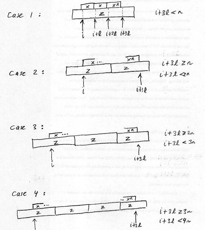
Figure 24: Cases of the argument

Case 1: If $xxx^{R}$ lies entirely within one copy of $z$, it also lies in $\bf r$, which we have already seen cannot happen, in Theorem 37. This case therefore cannot occur.

Case 2: We use the predicate

$$\exists i\ \exists\ell\ (i+3\ell\geq n)\ \wedge\ (i+3\ell<2n)\ \wedge\ (\forall j<\ell\ \operatorname{cmp}(i+j,i+\ell+j))\ \wedge\ (\forall k<\ell\ \operatorname{cmp}(i+k,i+3\ell-1-k))$$

to assert that there is a repetition of the form $xxx^{R}$.

Case 3: We use the predicate

$$\exists i\ \exists\ell\ (i+3\ell\geq 2n)\ \wedge\ (i+3\ell<3n)\ \wedge\ (\forall j<\ell\ \operatorname{cmp}(i+j,i+\ell+j-n))\ \wedge\ (\forall k<\ell\ \operatorname{cmp}(i+k,i+3\ell-1-k-n))).$$

Case 4: We use the predicate

$$\exists i\ \exists\ell\ (i+3\ell\geq 3n)\ \wedge\ (i+3\ell<4n)\ \wedge\ (\forall j<\ell\ \operatorname{cmp}(i+j,i+\ell+j-n))\ \wedge\ (\forall k<\ell\ \operatorname{cmp}(i+k,i+3\ell-1-k-2n)).$$

When we checked each of the cases 2 through 4 with our program, we discovered that $n=2F_{3k+2}$ is never accepted. Actually, for cases (2)–(4) we had to employ one additional trick, because the computation for the predicates as stated required more space than was available on our machine. Here is the additional trick: instead of attempting to run the predicate for all $n$, we ran it only for $n$ whose Fibonacci representation was of the form $10010^{*}$. This significantly restricted the size of the automata we created and allowed the computation to terminate. In fact, we propagated this condition throughout the predicate.

We therefore eliminated all possibilities for the occurrence of $xxx^{R}$ in $z^{\omega}$ and so it follows that no $xxx^{R}$ occurs in $z^{\omega}$. ∎

Open Problem 49.

How many binary words of length $n$ avoid the pattern $xxx^{R}$? Is it polynomial in $n$ or exponential? How about the number of binary words of length $n$ avoiding $xxx^{R}$ and simultaneously avoiding $(2+\alpha)$-powers?

Consider finite words of the form $xxx^{R}$ having no proper factor of the form $www^{R}$.

Conjecture 50.

For $n=F_{3k+1}$ there are $4$ such words of length $n$. For $n=F_{3k+1}\pm F_{3k-2}$ there are $2$ such words. Otherwise there are none.

For $k\geq 3$ the $4$ words of length $n=F_{3k+1}$ are given by ${\bf r}[p_{i}..p_{i}+n-1]$, $i=1,2,3,4$, where

$$(p_{1})_{F} =1000(010)^{k-3}001$$

$$(p_{2})_{F} =10(010)^{k-2}001$$

$$(p_{3})_{F} =1001000(010)^{k-3}001$$

$$(p_{4})_{F} =1010(010)^{k-2}001$$

For $k\geq 3$ the $2$ words of length $n=F_{3k+1}-F_{3k-2}$ are given by ${\bf r}[q_{i}..q_{i}+n-1]$, $i=1,2$, where

$$(q_{1})_{F} =10(010)^{k-3}001$$

$$(q_{2})_{F} =10000(010)^{k-3}001$$

For $k\geq 3$ the $2$ words of length $n=F_{3k+1}+F_{3k-2}$ are given by ${\bf r}[s_{i}..s_{i}+n-1]$, $i=1,2$, where

$$(s_{1})_{F} =10(010)^{k-3}001$$

$$(s_{2})_{F} =1000(01)^{k-2}001$$

6 Other sequences

In this section we briefly apply our method to some other Fibonacci-automatic sequences, obtaining several new results.

Consider a Fibonacci analogue of the Thue-Morse sequence

$${\bf v}=(v_{n})_{n\geq 0}=0111010010001100010111000101\cdots$$

where $v_{n}$ is the sum of the bits, taken modulo $2$, of the Fibonacci representation of $n$. This sequence was introduced in [72, Example 2, pp. 12–13].

We recall that an overlap is a word of the form $axaxa$ where $x$ may be empty; its order is defined to be $|ax|$. Similarly, a super-overlap is a word of the form $abxabxab$; an example of a super-overlap in English is the word tingalingaling with the first letter removed.

Theorem 51.

The only squares in $\bf v$ are of order $4$ and $F_{n}$ for $n\geq 2$, and a square of each such order occurs. The only cubes in $\bf v$ are the strings $000$ and $111$. The only overlaps in $\bf v$ are of order $F_{2n}$ for $n\geq 1$, and an overlap of each such order occurs. There are no super-overlaps in $\bf v$.

Proof.

As before. We omit the details. ∎

We might also like to show that $\bf v$ is recurrent. The obvious predicate for this property holding for all words of length $n$ is

$$\forall i\ \exists j\ ((j>i)\wedge(\forall t\ ((t<n)\implies({\bf v}[i+t]={\bf v}[j+t])))).$$

Unfortunately, when we attempt to run this with our prover, we get an intermediate NFA of 1159 states that we cannot determinize within the available space.

Instead, we rewrite the predicate, setting $k:=j-i$ and $u:=i+t$. This gives

$$\forall i\ \exists j\ (j>i)\wedge\forall k\ \forall u\ ((k\geq 1)\wedge(i=j+k)\wedge(u\geq i)\wedge(u<n+i))\implies{\bf v}[u]={\bf v}[u+k].$$

When we run this we discover that $\bf v$ is indeed recurrent. Here the computation takes a nontrivial 814007 ms, and the largest intermediate automaton has 625176 states. This proves

Theorem 52.

The word $\bf v$ is recurrent.

Another quantity of interest for the Thue-Morse-Fibonacci word $\bf v$ is its subword complexity $\rho_{\bf v}(n)$. It is not hard to see that it is linear. To obtain a deeper understanding of it, let us compute the first difference sequence $d(n)=\rho_{\bf v}(n+1)-\rho_{\bf v}(n)$. It is easy to see that $d(n)$ is the number of words $w$ of length $n$ with the property that both $w0$ and $w1$ appear in $\bf v$. The natural way to count this is to count those $i$ such that $t:={\bf v}[i..i+n-1]$ is the first appearance of that factor in $\bf v$, and there exists a factor ${\bf v}[k..k+n]$ of length $n+1$ whose length-$n$-prefix equals $t$ and whose last letter ${\bf v}[k+n]$ differs from ${\bf v}[i+n]$.

$$(\forall j<i\ \exists t<n\ {\bf v}[i+t]\not={\bf v}[j+t])\ \wedge\ (\exists k\ (\forall u<n\ {\bf v}[i+u]={\bf v}[k+u])\wedge{\bf v}[i+n]\not={\bf v}[k+n]).$$

Unfortunately the same blowup appears as in the recurrence predicate, so once agin we need to substitute, resulting in the predicate

$$(\forall j<i\ \exists k\geq 1\ \exists v\ (i=j+k)\wedge(v\geq j)\wedge(v<n+j)\wedge{\bf v}[u]\not={\bf v}[u+k])\wedge\\ (\exists l>i\ {\bf v}[i+n]\not={\bf v}[l+n])\wedge\\ (\forall k^{\prime}\ \forall u^{\prime}\ (k^{\prime}\geq 1)\wedge(l=i+k^{\prime})\wedge(u^{\prime}\geq i)\wedge(v^{\prime}<n+i)\implies{\bf v}[k^{\prime}+u^{\prime}]={\bf v}[u^{\prime}]).$$

From this we obtain a linear representation of rank $46$. We can now consider all vectors of the form $u\{M_{0},M_{1}\}^{*}$. There are only finitely many and we can construct an automaton out of them computing $d(n)$.

Theorem 53.

The first difference sequence $(d(n))_{n\geq 0}$ of the subword complexity of $\bf v$ is Fibonacci-automatic, and is accepted by the following machine.

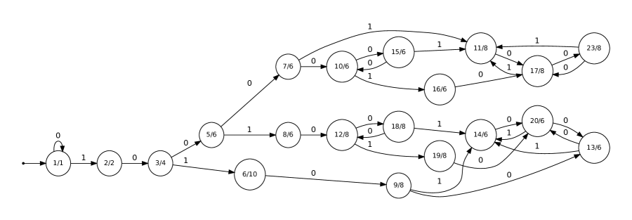
Figure 25: Automaton computing $d(n)$

7 Combining two representations and avoidability

In this section we show how our decidability method can be used to handle an avoidability question where two different representations arise.

Let $x$ be a finite word over the alphabet ${\mathbb{N}}^{*}=\{1,2,3\ldots\}$. We say that $x$ is an additive square if $x=x_{1}x_{2}$ with $|x_{1}|=|x_{n}|$ and $\sum x_{1}=\sum x_{2}$. For example, with the usual association of ${\tt a}=1$, ${\tt b}=2$, and so forth, up to ${\tt z}=26$, we have that the English word baseball is an additive square, as base and ball both sum to $27$.

An infinite word ${\bf x}$ over ${\mathbb{N}}^{*}$ is said to avoid additive squares if no factor is an additive square. It is currently unknown, and a relatively famous open problem, whether there exists an infinite word over a finite subset of ${\mathbb{N}}^{*}$ that avoids additive squares [15, 61, 49].., although it is known that additive cubes can be avoided over an alphabet of size $4$ [24]. (Recently this was improved to alphabet size $3$; see [65].)

However, it is easy to avoid additive squares over an infinite subset of ${\mathbb{N}}^{*}$; for example, any sequence that grows sufficiently quickly will have the desired property. Hence it is reasonable to ask about the lexicographically least sequence over ${\mathbb{N}}^{*}$ that avoids additive squares. Such a sequence begins

$$1213121421252131213412172\cdots,$$

but we do not even know if this sequence is unbounded.

Here we consider the following variation on this problem. Instead of considering arbitrary sequences, we start with a sequence ${\bf b}=b_{0}b_{1}b_{2}\cdots$ over ${\mathbb{N}}^{+}$ and from it construct the sequence $S({\bf b})=a_{1}a_{2}a_{3}\cdots$ defined by

$${\bf a}[i]={\bf b}[\nu_{2}(i)]$$

for $i\geq 1$, where $\nu_{2}(i)$ is the exponent of the largest power of $2$ dividing $i$. (Note that ${\bf a}$ and ${\bf b}$ are indexed differently.) For example, if ${\bf b}=123\cdots$, then ${\bf a}=1213121412131215\cdots$, the so-called “ruler sequence”. It is known that this sequence is squarefree and is, in fact, the lexicographically least sequence over ${\mathbb{N}}^{*}$ avoiding squares [48].

We then ask: what is the lexicographically least sequence avoiding additive squares that is of the form $S({\bf b})$? The following theorem gives the answer.

Theorem 54.

The lexicographically least sequence over ${\mathbb{N}}\setminus\{0\}$ of the form $S({\bf b})$ that avoids additive squares is defined by ${\bf b}[i]\mathrel{\mathop{:}}=F_{i+2}$.

Proof.

First, we show that ${\bf a}\mathrel{\mathop{:}}=S({\bf b})=\prod_{k=1}^{\infty}{\bf b}[\nu_{2}(k)]=\prod_{k=1}^{\infty}F_{\nu_{2}(k)+2}$ avoids additive squares.

For $m,n,j\in{\mathbb{N}}$, let $A(m,n,j)$ denote the number of occurrences of $j$ in $\nu_{2}(m+1),\dots,\nu_{2}(m+n)$.

(a): Consider two consecutive blocks of the same size say $a_{i+1}\cdots a_{i+n}$ and $a_{i+n+1}\cdots a_{i+2n}$. Our goal is to compare the sums $\sum_{i<j\leq i+n}a_{j}$ and $\sum_{i+n<j\leq i+2n}a_{j}$.

First we prove

Lemma 55.

Let $m,j\geq 0$ and $n\geq 1$ be integers. Let $A(m,n,j)$ denote the number of occurrences of $j$ in $\nu_{2}(m+1),\ldots,\nu_{2}(m+n)$. Then for all $m,m^{\prime}\geq 0$ we have $|A(m^{\prime},n,j)-A(m,n,j)|\leq 1$.

Proof.

We start by observing that the number of positive integers $\leq n$ that are divisible by $t$ is exactly $\lfloor n/t\rfloor$. It follows that the number $B(n,j)$ of positive integers $\leq n$ that are divisible by $2^{j}$ but not by $2^{j+1}$ is

$$B(n,j)=\lfloor{n\over{2^{j}}}\rfloor-\lfloor{n\over{2^{j+1}}}\rfloor.$$ (1)

Now from the well-known identity

$$\lfloor x\rfloor+\lfloor x+{1\over 2}\rfloor=\lfloor 2x\rfloor,$$

valid for all real numbers $x$, substitute $x=n/2^{j+1}$ to get

$$\lfloor{n\over{2^{j+1}}}\rfloor+\lfloor{n\over{2^{j+1}}}+{1\over 2}\rfloor=\lfloor{n\over{2^{j}}}\rfloor,$$

which, combined with (1), shows that

$$B(n,j)=\lfloor{n\over{2^{j+1}}}+{1\over 2}\rfloor.$$

Hence

$${n\over{2^{j+1}}}-{1\over 2}\leq B(n,j)<{n\over{2^{j+1}}}+{1\over 2}.$$ (2)

Now the number of occurrences of $j$ in $\nu_{2}(m+1),\ldots,\nu_{2}(m+n)$ is $A(m,n,j)=B(m+n,j)-B(m,j)$. From (2) we get

$${n\over{2^{j+1}}}-1<A(m,n,j)<{n\over{2^{j+1}}}+1$$ (3)

for all $m\geq 0$. Since $A(m,n,j)$ is an integer, the inequality (3) implies that $|A(m^{\prime},n,j)-A(m,n,j)|\leq 1$ for all $m,m^{\prime}$. ∎

Note that for all $i,n\in{\mathbb{N}}$, we have $\sum_{k=i}^{i+n-1}{\bf a}[k]=\sum_{j=0}^{\left\lfloor\log_{2}(i+n)\right\rfloor}A(i,n,j)F_{j+2}$, so for adjacent blocks of length $n$, $\sum_{k=i+n}^{i+2n-1}{\bf a}[k]-\sum_{k=i}^{i+n-1}{\bf a}[k]=\sum_{j=0}^{\left\lfloor\log_{2}(i+2n)\right\rfloor}(A(i+n,n,j)-A(i,n,j))F_{j+2}$. Hence, ${\bf a}[i\ldotp\ldotp i+2n-1]$ is an additive square iff $\sum_{j=0}^{\left\lfloor\log_{2}(i+2n)\right\rfloor}(A(i+n,n,j)-A(i,n,j))F_{j+2}=0$, and by above, each $A(i+n,n,j)-A(i,n,j)\in\{-1,0,1\}$.

The above suggests that we can take advantage of “unnormalized” Fibonacci representation in our computations. For $\Sigma\subseteq{\mathbb{Z}}$ and $w\in\Sigma^{*}$, we let the unnormalized Fibonacci representation $\left\langle w\right\rangle_{uF}$ be defined in the same way as $\left\langle w\right\rangle_{F}$, except over the alphabet $\Sigma$.

In order to use Procedure 3, we need two auxiliary DFAs: one that, given $i,n\in{\mathbb{N}}$ (in any representation; we found that base 2 works), computes $\left\langle A(i+n,n,\_)-A(i,n,\_)\right\rangle_{uF}$, and another that, given $w\in\{{\tt-1},{\tt 0},{\tt 1}\}^{*}$, decides whether $\left\langle w\right\rangle_{uF}=0$. The first task can be done by a 6-state (incomplete) DFA $M_{\text{add22F}}$ that accepts the language $\{z\in(\Sigma_{2}^{2}\times\{{\tt-1},{\tt 0},{\tt 1}\})^{*}\;:\;\forall j(\pi_{3}(z)[j]=A(\left\langle\pi_{1}(z)\right\rangle_{2}+\left\langle\pi_{2}(z)\right\rangle_{2},\left\langle\pi_{2}(z)\right\rangle_{2},j)-A(\left\langle\pi_{1}(z)\right\rangle_{2},\left\langle\pi_{2}(z)\right\rangle_{2},j))\}$. The second task can be done by a 5-state (incomplete) DFA $M_{\text{1uFisZero}}$ that accepts the language $\{w\in\{{\tt-1},{\tt 0},{\tt 1}\}^{*}\;:\;\left\langle w\right\rangle_{uF}=0\}$.

We applied a modified Procedure 3 to the predicate $n\geq 1\wedge\exists w({\tt add22F}(i,n,w)\wedge{\tt 1uFisZero}(w))$ and obtained as output a DFA that accepts nothing, so ${\bf a}$ avoids additive squares.

Next, we show that ${\bf a}$ is the lexicographically least sequence over ${\mathbb{N}}\setminus\{0\}$ of the form $S({\bf b})$ that avoids additive squares.

Note that for all ${\bf x},{\bf y}\in{\mathbb{N}}\setminus\{0\}$, $S({\bf x})<S({\bf y})$ iff ${\bf x}<{\bf y}$ in the lexicographic ordering. Thus, we show that if any entry ${\bf b}[s]$ with ${\bf b}[s]>1$ is changed to some $t\in[1,{\bf b}[s]-1]$, then ${\bf a}=S({\bf b})$ contains an additive square using only the first occurrence of the change at ${\bf a}[2^{s}-1]$. More precisely, we show that for all $s,t\in{\mathbb{N}}$ with $t\in[1,F_{s+2}-1]$, there exist $i,n\in{\mathbb{N}}$ with $n\geq 1$ and $i+2n<2^{s+1}$ such that either ($2^{s}-1\in[i,i+n-1]$ and $\sum_{k=i+n}^{i+2n-1}{\bf a}[k]-\sum_{k=i}^{i+n-1}{\bf a}[k]+t=0$) or ($2^{s}-1\in[i+n,i+2n-1]$ and $\sum_{k=i+n}^{i+2n-1}{\bf a}[k]-\sum_{k=i}^{i+n-1}{\bf a}[k]-t=0$).

Setting up for a modified Procedure 3, we use the following predicate, which says “$r$ is a power of $2$ and changing ${\bf a}[r-1]$ to any smaller number results in an additive square in the first $2r$ positions”, and six auxiliary DFAs. Note that all arithmetic and comparisons are in base 2.

$${\tt powOf2}(r)\wedge\forall t((t\geq 1\wedge t<r\wedge{\tt canonFib}(t))\rightarrow\exists i\exists n(n\geq 1\wedge i+2n<2r\wedge{}$$

$$\quad((i<r\wedge r\leq i+n\wedge\forall w({\tt add22F}(i,n,w)\rightarrow\forall x({\tt bitAdd}(t,w,x)\rightarrow{\tt 2uFisZero}(x))))\vee{}$$

$$\quad\hphantom{(}(i+n<r\wedge r\leq i+2n\wedge\forall w({\tt add22F}(i,n,w)\rightarrow\forall x({\tt bitSub}(t,w,x)\rightarrow{\tt 2uFisZero}(x))))))).$$

$$L(M_{\text{powOf2}}) =\{w\in\Sigma_{2}^{*}\;:\;\exists n(w=(2^{n})_{2})\}.$$

$$L(M_{\text{canonFib}}) =\{w\in\Sigma_{2}^{*}\;:\;\exists n(w=(n)_{F})\}.$$

$$L(M_{\text{bit(Add/Sub)}}) =\{z\in(\Sigma_{2}\times\{{\tt-1},{\tt 0},{\tt 1}\}\times\{{\tt-1},{\tt 0},{\tt 1},{\tt 2}\})^{*}\;:\;\forall i(\pi_{1}(z)[i]\pm\pi_{2}(z)[i]=\pi_{3}(z)[i])\}.$$

$$L(M_{\text{2uFisZero}}) =\{w\in\{{\tt-1},{\tt 0},{\tt 1},{\tt 2}\}^{*}\;:\;\left\langle w\right\rangle_{uF}=0\}.$$

We applied a modified Procedure 3 to the above predicate and auxiliary DFAs and obtained as output $M_{\text{powOf2}}$, so ${\bf a}$ is the lexicographically least sequence over ${\mathbb{N}}\setminus\{0\}$ of the form $S({\bf b})$ that avoids additive squares. ∎

8 Enumeration

Mimicking the base-$k$ ideas in [25], we can also mechanically enumerate many aspects of Fibonacci-automatic sequences. We do this by encoding the factors having the property in terms of paths of an automaton. This gives the concept of Fibonacci-regular sequence as previously studied in [3]. Roughly speaking, a sequence $(a(n))_{n\geq 0}$ taking values in ${\mathbb{N}}$ is Fibonacci-regular if the set of sequences

$$\{(a([xw]_{F})_{w\in\Sigma_{2}^{*}}\ :\ x\in\Sigma_{2}^{*}\}$$

is finitely generated. Here we assume that $a([xw]_{F})$ evaluates to $0$ if $xw$ contains the string $11$. Every Fibonacci-regular sequence $(a(n))_{n\geq 0}$ has a linear representation of the form $(u,\mu,v)$ where $u$ and $v$ are row and column vectors, respectively, and $\mu:\Sigma_{2}\rightarrow{\mathbb{N}}^{d\times d}$ is a matrix-valued morphism, where $\mu(0)=M_{0}$ and $\mu(1)=M_{1}$ are $d\times d$ matrices for some $d\geq 1$, such that

$$a(n)=u\cdot\mu(x)\cdot v$$

whenever $[x]_{F}=n$. The rank of the representation is the integer $d$. As an example, we exhibit a rank-$6$ linear representation for the sequence $a(n)=n+1$:

$$u =[1\ 2\ 2\ 3\ 3\ 2]$$

$$M_{0} =\left[\begin{array}[]{cccccc}1&1&0&0&0&0\\ 0&0&0&0&0&0\\ 0&1&0&1&1&0\\ 0&0&1&1&1&1\\ 0&0&0&0&0&0\\ 0&0&0&0&0&0\end{array}\right]$$

$$M_{1} =\left[\begin{array}[]{cccccc}0&0&0&0&0&0\\ 1&0&0&0&0&0\\ 0&0&0&0&0&0\\ 0&0&0&0&0&0\\ 0&0&1&1&0&0\\ 0&0&0&1&0&0\end{array}\right]$$

$$v =[1\ 0\ 0\ 0\ 0\ 0]^{T}.$$

This can be proved by a simple induction on the claim that

$$u\cdot\mu(x)=[x_{F}+1\ (1x)_{F}+1\ (10x)_{F}-x_{F}\ (100x)_{F}-x_{F}\ (101x)_{F}-(1x)_{F}\ (1001x)_{F}-(101x)_{F}]$$

for strings $x$.

Recall that if $\bf x$ is an infinite word, then the subword complexity function $\rho_{\bf x}(n)$ counts the number of distinct factors of length $n$. Then, in analogy with [25, Thm. 27], we have

Theorem 56.

If $\bf x$ is Fibonacci-automatic, then the subword complexity function of $\bf x$ is Fibonacci-regular.

Using our implementation, we can obtain a linear representation of the subword complexity function for $\bf f$. To do so, we use the predicate

$$\{(n,i)_{F}\ :\ \forall i^{\prime}<i\ {\bf f}[i..i+n-1]\not={\bf f}[i^{\prime}..i^{\prime}+n-1]\},$$

which expresses the assertion that the factor of length $n$ beginning at position $i$ has never appeared before. Then, for each $n$, the number of corresponding $i$ gives $\rho_{\bf f}(n)$. When we do this for $\bf f$, we get the following linear representation $(u^{\prime},\mu^{\prime},v^{\prime})$ of rank $10$:

$$u^{\prime} =[0\ 0\ 0\ 1\ 0\ 0\ 0\ 0\ 0\ 0]$$

$$M^{\prime}_{0} =\left[\begin{array}[]{ccccccccccc}0&1&1&0&0&0&0&0&0&0\\ 0&0&0&0&0&0&0&0&0&0\\ 1&0&0&0&0&0&0&0&0&0\\ 0&0&0&1&0&0&0&0&0&0\\ 1&0&0&0&0&1&0&0&0&0\\ 0&0&0&0&0&0&0&1&0&0\\ 0&0&0&0&0&1&0&1&0&0\\ 0&0&0&0&0&1&0&1&0&0\\ 1&0&0&0&0&0&0&0&0&0\\ 0&0&0&0&0&0&0&1&0&0\end{array}\right]$$

$$M^{\prime}_{1} =\left[\begin{array}[]{ccccccccccc}0&0&0&0&1&0&0&0&0&1\\ 0&0&0&0&0&0&0&0&1&0\\ 0&0&0&0&0&0&1&0&0&0\\ 0&0&0&0&0&0&1&0&1&0\\ 0&0&0&0&0&0&0&0&0&0\\ 0&0&0&0&0&0&1&0&0&0\\ 0&0&0&0&0&0&0&0&0&0\\ 0&0&0&0&0&0&1&0&0&1\\ 0&0&0&0&0&0&0&0&0&0\\ 0&0&0&0&0&0&0&0&0&0\end{array}\right]$$

$$v^{\prime} =[1\ 0\ 1\ 1\ 1\ 1\ 1\ 1\ 1\ 1]^{T}$$

To show that this computes the function $n+1$, it suffices to compare the values of the linear representations $(u,\mu,v)$ and $(u^{\prime},\mu^{\prime},v^{\prime})$ for all strings of length $\leq 10+6=16$ (using [8, Corollary 3.6]). After checking this, we have reproved the following classic theorem of Morse and Hedlund [58]:

Theorem 57.

The subword complexity function of $\bf f$ is $n+1$.

We now turn to a result of Fraenkel and Simpson [39]. They computed the exact number of squares appearing in the finite Fibonacci words $X_{n}$; this was previously estimated by [29].

There are two variations: we could count the number of distinct squares in $X_{n}$, or what Fraenkel and Simpson called the number of “repeated squares” in $X_{n}$ (i.e., the total number of occurrences of squares in $X_{n}$).

To solve this using our approach, we generalize the problem to consider any length-$n$ prefix of $X_{n}$, and not simply the prefixes of length $F_{n}$.

We can easily write down predicates for these. The first represents the number of distinct squares in ${\bf f}[0..n-1]$:

$$L_{\rm ds}:=\{(n,i,j)_{F}\ :\ (j\geq 1)\text{ and }(i+2j\leq n)\text{ and }{\bf f}[i..i+j-1]={\bf f}[i+j..i+2j-1]\\ \text{ and }\forall i^{\prime}<i\ {\bf f}[i^{\prime}..i^{\prime}+2j-1]\not={\bf f}[i..i+2j-1]\}.$$

This predicate asserts that ${\bf f}[i..i+2j-1]$ is a square occurring in ${\bf f}[0..n-1]$ and that furthermore it is the first occurrence of this particular string in ${\bf f}[0..n-1]$.

The second represents the total number of occurrences of squares in ${\bf f}[0..n-1]$:

$$L_{\rm dos}:=\{(n,i,j)_{F}\ :\ (j\geq 1)\text{ and }(i+2j\leq n)\text{ and }{\bf f}[i..i+j-1]={\bf f}[i+j..i+2j-1]\}.$$

This predicate asserts that ${\bf f}[i..i+2j-1]$ is a square occurring in ${\bf f}[0..n-1]$.

We apply our method to the second example, leaving the first to the reader. Let $b(n)$ denote the number of occurrences of squares in ${\bf f}[0..n-1]$. First, we use our method to find a DFA $M$ accepting $L_{\rm dos}$. This (incomplete) DFA has 27 states.

Next, we compute matrices $M_{0}$ and $M_{1}$, indexed by states of $M$, such that $(M_{a})_{k,l}$ counts the number of edges (corresponding to the variables $i$ and $j$) from state $k$ to state $l$ on the digit $a$ of $n$. We also compute a vector $u$ corresponding to the initial state of $M$ and a vector $v$ corresponding to the final states of $M$. This gives us the following linear representation of the sequence $b(n)$: if $x=a_{1}a_{2}\cdots a_{t}$ is the Fibonacci representation of $n$, then

$$b(n)=uM_{a_{1}}\cdots M_{a_{t}}v,$$ (4)

which, incidentally, gives a fast algorithm for computing $b(n)$ for any $n$.

Now let $B(n)$ denote the number of square occurrences in the finite Fibonacci word $X_{n}$. This corresponds to considering the Fibonacci representation of the form $10^{n-2}$; that is, $B(n+1)=b([10^{n-1}]_{F})$. The matrix $M_{0}$ is the following $27\times 27$ array

$$\left[\begin{array}[]{ccccccccccccccccccccccccccc}1&1&0&0&0&0&0&0&0&0&0&0&0&0&0&0&0&0&0&1&0&0&0&0&0&0&0\\ 1&0&0&0&0&0&0&0&0&0&0&0&0&0&0&0&0&0&0&0&1&0&0&0&0&0&0\\ 1&0&0&0&0&0&0&0&0&0&0&0&0&0&0&1&0&0&0&0&0&0&0&0&0&0&0\\ 0&0&0&0&0&0&0&0&0&0&0&0&0&0&0&0&0&0&0&0&1&0&0&0&0&0&0\\ 0&0&0&0&0&0&0&0&0&0&0&0&0&0&0&0&0&0&0&0&0&0&0&0&0&0&1\\ 1&0&0&0&0&0&0&0&0&0&0&0&0&0&0&1&0&0&0&0&0&0&0&0&0&0&0\\ 0&0&0&0&0&0&0&0&0&0&0&0&0&0&0&1&0&0&0&0&0&0&1&0&0&0&0\\ 0&0&0&0&0&0&0&0&0&0&0&0&0&0&0&0&0&1&0&0&0&0&0&0&0&0&0\\ 0&0&0&1&0&0&0&0&0&0&0&0&0&0&0&0&0&0&0&0&1&0&0&0&0&0&0\\ 0&0&0&0&0&0&0&0&0&0&0&0&0&0&0&0&0&1&0&0&0&0&0&0&0&0&0\\ 1&0&0&0&0&1&0&0&0&0&0&0&0&0&0&0&0&0&0&1&0&0&0&0&0&0&0\\ 0&0&0&0&0&0&0&0&0&0&0&0&0&0&0&0&0&0&0&0&0&0&0&0&0&0&0\\ 1&1&0&0&0&0&0&0&0&0&0&0&0&0&0&0&0&0&0&1&0&0&0&0&0&0&0\\ 0&0&0&0&0&0&0&0&0&0&1&0&0&0&0&0&0&0&0&0&0&0&1&0&0&1&0\\ 0&0&0&0&0&0&0&0&0&0&0&0&0&0&0&0&0&0&0&1&1&0&0&0&0&0&0\\ 0&0&0&0&0&0&0&0&0&1&0&0&0&0&0&0&0&0&0&0&1&0&0&0&0&0&0\\ 1&0&0&0&0&0&0&0&0&0&0&0&0&0&0&0&0&0&0&0&1&0&0&0&0&0&0\\ 0&0&0&0&0&0&0&0&0&0&0&0&0&0&0&0&0&1&0&0&0&0&0&0&0&0&0\\ 0&0&0&0&0&0&0&0&0&0&1&0&0&0&0&0&0&0&0&0&0&0&1&0&0&1&0\\ 0&0&0&0&0&0&0&0&0&0&0&0&0&0&0&0&0&0&0&0&0&0&0&0&0&0&1\\ 0&0&0&1&0&0&0&0&0&0&0&0&0&0&0&0&0&0&0&0&1&0&0&0&0&0&0\\ 0&0&0&0&0&0&0&0&0&0&0&0&0&0&0&0&0&0&0&0&0&1&0&0&0&0&0\\ 0&0&0&0&0&0&0&0&0&0&0&1&0&0&0&0&0&0&0&0&0&0&0&0&0&0&0\\ 0&0&0&0&0&0&0&0&0&0&0&0&0&0&0&0&0&0&0&0&0&1&0&0&0&0&0\\ 0&0&0&0&0&0&0&0&0&0&0&0&0&0&0&0&0&0&0&0&1&0&0&0&0&0&0\\ 0&0&0&0&0&0&0&0&0&0&0&0&0&0&0&0&0&0&1&0&0&0&0&0&0&0&0\\ 0&0&0&0&0&0&0&0&0&0&0&0&0&0&0&0&0&0&0&1&1&0&0&0&0&0&0\end{array}\right]$$ (5)

and has minimal polynomial

$$X^{4}(X-1)^{2}(X+1)^{2}(X^{2}-X-1)^{2}.$$

It now follows from the theory of linear recurrences that there are constants $c_{1},c_{2},\ldots,c_{8}$ such that

$$B(n+1)=(c_{1}n+c_{2})\alpha^{n}+(c_{3}n+c_{4})\beta^{n}+c_{5}n+c_{6}+(c_{7}n+c_{8})(-1)^{n}$$

for $n\geq 3$, where $\alpha=(1+\sqrt{5})/2$, $\beta=(1-\sqrt{5})/2$ are the roots of $X^{2}-X-1$. We can find these constants by computing $B(4),B(5),\ldots,B(11)$ (using Eq. (4)) and then solving for the values of the constants $c_{1},\ldots,c_{8}$.

When we do so, we find

$$c_{1} ={2\over 5}\quad\quad c_{2} ={-{2\over{25}}}\sqrt{5}-2$$

$$c_{3} ={2\over 5}\quad\quad c_{4} ={{2\over{25}}}\sqrt{5}-2$$

$$c_{5} =1\quad\quad c_{6} =1$$

$$c_{7} =0\quad\quad c_{8} =0$$

A little simplification, using the fact that $F_{n}=(\alpha^{n}-\beta^{n})/(\alpha-\beta)$, leads to

Theorem 58.

Let $B(n)$ denote the number of square occurrences in $X_{n}$. Then

$$B(n+1)={4\over 5}nF_{n+1}-{2\over 5}(n+6)F_{n}-4F_{n-1}+n+1$$

for $n\geq 3$.

This statement corrects a small error in Theorem 2 in [39] (the coefficient of $F_{n-1}$ was wrong; note that their $F$ and their Fibonacci words are indexed differently from ours), which was first pointed out to us by Kalle Saari.

In a similar way, we can count the cube occurrences in $X_{n}$. Using analysis exactly like the square case, we easily find

Theorem 59.

Let $C(n)$ denote the number of cube occurrences in the Fibonacci word $X_{n}$. Then for $n\geq 3$ we have

$$C(n)=(d_{1}n+d_{2})\alpha^{n}+(d_{3}n+d_{4})\beta^{n}+d_{5}n+d_{6}$$

where

$$d_{1} ={{3-\sqrt{5}}\over{10}}\quad\quad d_{2} ={{17}\over{50}}\sqrt{5}-{3\over 2}$$

$$d_{3} ={{3+\sqrt{5}}\over{10}}\quad\quad d_{4} =-{{17}\over{50}}\sqrt{5}-{3\over 2}$$

$$d_{5} =1\quad\quad d_{6} =-1.$$

We now turn to a question of Chuan and Droubay. Let us consider the prefixes of $\bf f$. For each prefix of length $n$, form all of its $n$ shifts, and let us count the number of these shifts that are palindromes; call this number $d(n)$. (Note that in the case where a prefix is a power, two different shifts could be identical; we count these with multiplicity.)

Chuan [27, Thm. 7, p. 254] proved

Theorem 60.

For $i>2$ we have $d(F_{i})=0$ iff $i\equiv 0\ ({\rm mod}\ 3)$.

Proof.

Along the way we actually prove a lot more, characterizing $d(n)$ for all $n$, not just those $n$ equal to a Fibonacci number.

We start by showing that $d(n)$ takes only three values: $0$, $1$, and $2$. To do this, we construct an automaton accepting the language

$$\{(n,i)_{F}\ :\ (0\leq i<n)\ \wedge\ {\bf f}[i..n-1]{\bf f}[0..i-1]\text{ is a palindrome }\}.$$

From this we construct the linear representation $(u,M_{0},M_{1},v)$ of $d(n)$ as discussed above; it has rank $27$.

The range of $c$ is finite if the monoid ${\cal M}=\langle M_{0},M_{1}\rangle$ is finite. This can be checked with a simple queue-based algorithm, and $\cal M$ turns out to have cardinality $151$. From these a simple computation proves

$$\{uMv\ :\ M\in{\cal M}\}=\{0,1,2\},$$

and so our claim about the range of $c$ follows.

Now that we know the range of $c$ we can create predicates $P_{0}(n),P_{1}(n),P_{2}(n)$ asserting that (a) there are no length-$n$ shifts that are palindromes (b) there is exactly one shift that is a palindrome and (c) more than one shift is a palindrome, as follows:

$$P_{0}:\neg\exists i,(0\leq i<n),{\bf f}[i..n-1]{\bf f}[0..i-1]\text{ is a palindrome }$$

$$P_{1}:\exists i,(0\leq i<n),{\bf f}[i..n-1]{\bf f}[0..i-1]\text{ is a palindrome and }\neg\exists j\not=i(0\leq j<n),{\bf f}[j..n-1]{\bf f}[0..j-1]$$

$$P_{2}:\exists i,j,0\leq i<j<n{\bf f}[i..n-1]{\bf f}[0..i-1]\text{ and }{\bf f}[j..n-1]{\bf f}[0..j-1]\text{ are both palindromes }$$

For each one, we can compute a finite automaton characterizing the Fibonacci representations of those $n$ for which $d(n)$ equals, respectively, $0$, $1$, and $2$.

For example, we computed the automaton corresponding to $P_{0}$, and it is displayed in Figure 26 below.

Figure 26: Automaton accepting lengths of prefixes for which no shifts are palindromes

By tracing the path labeled $10^{*}$ starting at the initial state labeled $18$, we see that the “finality” of the states encountered is ultimately periodic with period $3$, proving Theorem 60. ∎

To finish this section, we reprove a result of Kolpakov and Kucherov [54]. Recalling the definition of maximal repetition from Section 3.1, they counted the number $\operatorname{mr}(F_{n})$ of occurrences of maximal repetitions in the prefix of $\bf f$ of length $F_{n}$:

Theorem 61.

For $n\geq 5$ we have $\operatorname{mr}(F_{n})=2F_{n-2}-3$.

Proof.

We create an automaton for the language

$$\{(n,i,j)_{F}\ :\ 0\leq i\leq j<n\text{ and }{\bf f}[i..j]\text{ is a maximal repetition of }{\bf f}[0..n-1]\},$$

using the predicate

$$(i\leq j)\ \wedge\ (j<n)\ \wedge\ \exists p\text{ with }1\leq p\leq(j+1-i)/2\text{ such that }\\ ((\forall k\leq j-i-p\ {\bf f}[i+k]={\bf f}[i+k+p])\ \wedge\ \\ (i\geq 1)\implies(\forall q\text{ with }1\leq q\leq p\ \exists\ell\leq j-i-q+1\ {\bf f}[i-i+\ell]\not={\bf f}[i-1+\ell+q])\ \wedge\ \\ (j+1\leq n-1)\implies(\forall r\text{ with }1\leq r\leq p\ \exists m\leq j+1-r-i\ {\bf f}[i+m]\not={\bf f}[i+m+r])).$$

Here the second line of the predicate specifies that there is a period $p$ of ${\bf f}[i..j]$ corresponding to a repetition of exponent at least $2$. The third line specifies that no period $q$ of ${\bf f}[i-1..j]$ (when this makes sense) can be $\leq p$, and the fourth line specifies that no period $r$ of ${\bf f}[i..j+1]$ (when $j+1\leq n-1$) can be $\leq p$.

From the automaton we deduce a linear representation $(u,\mu,v)$ of rank 59. Since $(F_{n})_{F}=10^{n-2}$, it suffices to compute the minimal polynomial of $M_{0}=\mu(0)$. When we do this, we discover it is $X^{4}(X^{2}-X-1)(X-1)^{2}(X+1)^{2}$. It follows from the theory of linear recurrences that

$$\operatorname{mr}(F_{n})=e_{1}\alpha^{n}+e_{2}\beta^{n}+e_{3}n+e_{4}+(e_{5}n+e_{6})(-1)^{n}$$

for constants $e_{1},e_{2},e_{3},e_{4},e_{5},e_{6}$ and $n\geq 6$. When we solve for $e_{1},\ldots,e_{6}$ by using the first few values of $\operatorname{mr}(F_{n})$ (computed from the linear representation or directly) we discover that $e_{1}=(3\sqrt{5}-5)/5$, $e_{2}=(-3\sqrt{5}-5)/5$, $e_{3}=e_{5}=e_{6}=0$, and $e_{4}=-3$. From this the result immediately follows. ∎

In fact, we can prove even more.

Theorem 62.

For $n\geq 0$ the difference $\operatorname{mr}(n+1)-\operatorname{mr}(n)$ is either $0$ or $1$. Furthermore there is a finite automaton with 10 states that accepts $(n)_{F}$ precisely when $\operatorname{mr}(n+1)-\operatorname{mr}(n)=1$.

Proof.

Every maximal repetition ${\bf f}[i..j]$ of ${\bf f}[0..n-1]$ is either a maximal repetition of ${\bf f}[0..n]$ with $j\leq n-1$, or is a maximal repetition with $j=n-1$ that, when considered in ${\bf f}[0..n]$, can be extended one character to the right to become one with $j=n$. So the only maximal repetitions of ${\bf f}[0..n]$ not (essentially) counted by $\operatorname{mr}(n)$ are those such that

$${\bf f}[i..n]\text{ is a maximal repetition of }{\bf f}[0..n]\text{ and }\\ {\bf f}[i..n-1]\text{ is {\it not\/} a maximal repetition of }{\bf f}[0..n-1].$$ (6)

We can easily create a predicate asserting this latter condition, and from this obtain the linear representation of $\operatorname{mr}(n+1)-\operatorname{mr}(n)$:

$$u =[0\ 0\ 0\ 0\ 0\ 1\ 0\ 0\ 0\ 0\ 0\ 0\ ]$$

$$\mu(0) =\left[\begin{array}[]{cccccccccccc}0&0&0&0&0&0&0&0&0&1&0&0\\ 0&0&0&0&0&0&0&0&0&0&1&0\\ 0&0&0&1&0&0&0&0&0&1&0&0\\ 0&0&0&0&0&0&0&1&0&0&0&0\\ 0&0&0&0&0&0&0&0&0&0&0&0\\ 0&0&0&0&0&1&0&0&0&0&0&0\\ 0&0&0&0&0&0&0&0&0&0&1&0\\ 0&0&0&0&1&0&0&0&0&0&0&0\\ 0&0&0&0&1&0&0&0&0&0&0&0\\ 0&0&0&0&0&0&0&0&0&0&0&1\\ 0&0&0&0&0&0&1&0&0&0&0&0\\ 0&0&0&0&0&0&0&0&0&1&0&0\end{array}\right]$$

$$\mu(1) =\left[\begin{array}[]{cccccccccccc}0&0&0&0&0&0&0&0&0&0&0&0\\ 0&0&0&0&0&0&0&0&0&0&0&0\\ 0&0&0&0&0&0&0&0&0&0&0&0\\ 0&0&0&0&0&0&0&0&0&0&0&0\\ 0&0&0&0&0&0&0&0&1&0&0&0\\ 0&1&1&0&0&0&0&0&0&0&0&0\\ 1&1&0&0&0&0&0&0&0&0&0&0\\ 0&0&0&0&0&0&0&0&0&0&0&0\\ 0&0&0&0&0&0&0&0&0&0&0&0\\ 0&0&0&0&0&0&0&0&0&0&0&0\\ 0&1&1&0&0&0&0&0&0&0&0&0\\ 0&0&0&0&0&0&0&0&1&0&0&0\end{array}\right]$$

$$v =[0\ 0\ 0\ 0\ 1\ 0\ 0\ 0\ 1\ 0\ 0\ 1]$$

We now use the trick we previously used for the proof of Theorem 60; the monoid generated by $\mu(0)$ and $\mu(1)$ has size $61$ and for each matrix $M$ in this monoid we have $uMv\in\{0,1\}$. It follows that $\operatorname{mr}(n+1)-\operatorname{mr}(n)\in\{0,1\}$ for all $n\geq 0$.

Knowing this, we can now build an automaton accepting those $n$ for which there exists an $i$ for which (6) holds. When we do so we get the automaton depicted below in Figure 27.

Figure 27: Automaton accepting $(n)_{F}$ such that $\operatorname{mr}(n+1)-\operatorname{mr}(n)=1$

∎

9 Abelian properties

Our decision procedure does not apply, in complete generality, to abelian properties of infinite words. This is because there is no obvious way to express assertions like $\psi(x)=\psi(x^{\prime})$ for two factors $x,x^{\prime}$ of an infinite word. (Here $\psi:\Sigma^{*}\rightarrow{\mathbb{N}}^{|\Sigma|}$ is the Parikh map that sends a word to the number of occurrences of each letter.) Indeed, in the $2$-automatic case it is provable that there is at least one abelian property that is inexpressible [69, §5.2].

However, the special nature of the Fibonacci word $\bf f$ allows us to mechanically prove some assertions involving abelian properties. In this section we describe how we did this.

By an abelian square of order $n$ we mean a factor of the form $xx^{\prime}$ where $\psi(x)=\psi(x^{\prime})$, where $n=|x|$. In a similar way we can define abelian cubes and higher powers.

We start with the elementary observation that $\bf f$ is defined over the alphabet $\{0,1\}$. Hence, to understand the abelian properties of a factor $x$ it suffices to know $|x|$ and $|x|_{0}$. Next, we observe that the map that sends $n$ to $a_{n}:=|{\bf f}[0..n-1]|_{0}$ (that is, the number of $0$’s in the length-$n$ prefix of $\bf f$), is actually synchronized (see [22, 20, 21, 47]). That is, there is a DFA accepting the Fibonacci representation of the pairs $(n,a_{n})$. In fact we have the following

Theorem 63.

Suppose the Fibonacci representation of $n$ is $e_{1}e_{2}\cdots e_{i}$. Then $a_{n}=[e_{1}e_{2}\cdots e_{i-1}]_{F}+e_{i}$.

Proof.

First, we observe that an easy induction on $m$ proves that $|X_{m}|_{0}=F_{m-1}$ for $m\geq 2$. We will use this in a moment.

The theorem’s claim is easily checked for $n=0,1$. We prove it for $F_{m+1}\leq n<F_{m+2}$ by induction on $m$. The base case is $m=1$, which corresponds to $n=1$.

Now assume the theorem’s claim is true for $m-1$; we prove it for $m$. Write $(n)_{F}=e_{1}e_{2}\cdots e_{m}$. Then, using the fact that ${\bf f}[0..F_{m+2}-1]=X_{m+2}=X_{m+1}X_{m}$, we get

$$|{\bf f}[0..n-1]|_{0} =|{\bf f}[0..F_{m+1}-1]|_{0}+|{\bf f}[F_{m+1}..n-1]|_{0}$$

$$=|X_{m+1}|_{0}+|{\bf f}[0..n-1-F_{m+1}]|_{0}$$

$$=F_{m}+|{\bf f}[0..n-1-F_{m+1}|_{0}$$

$$=F_{m}+[e_{2}\cdots e_{m-1}]_{F}+e_{m}$$

$$=[e_{1}\cdots e_{m-1}]_{F}+e_{m},$$

as desired. ∎

In fact, the synchronized automaton for $(n,a_{n})_{F}$ is given in the following diagram:

Figure 28: Automaton accepting $(n,a_{n})_{F}$

Here the missing state numbered $2$ is a “dead” state that is the target of all undrawn transitions.

The correctness of this automaton can be checked using our prover. Letting $\operatorname{ZC}(x,y)$ denote $1$ if $(x,y)_{F}$ is accepted, it suffices to check that

1. $\forall x\ \exists y\ \operatorname{ZC}(x,y)=1$ (that is, for each $x$ there is at least one corresponding $y$ accepted);

2. $\forall x\ \forall y\ \forall z\ (\operatorname{ZC}(x,y)=\operatorname{ZC}(x,z))\implies y=z$ (that is, for each $x$ at most one corresponding $y$ is accepted);

3. $\forall x\ \forall y\ ((\operatorname{ZC}(x,y)=1)\ \wedge\ ({\bf f}[x]=1))\implies(\operatorname{ZC}(x+1,y+1)=1)$;

4. $\forall x\ \forall y\ ((\operatorname{ZC}(x,y)=1)\ \wedge\ ({\bf f}[x]=0))\implies(\operatorname{ZC}(x+1,y)=1)$;

Another useful automaton computes, on input $n,i,j$ the function

$$\operatorname{FAB}(n,i,j):=|{\bf f}[i..i+n-1]|_{0}-|{\bf f}[j..j+n-1]|_{0}=a_{i+n}-a_{i}-a_{j+n}+a_{j}.$$

From the known fact that the factors of $\bf f$ are “balanced” we know that $\operatorname{FAB}$ takes only the values $-1,0,1$. This automaton can be deduced from the one above. However, we calculated it by “guessing” the right automaton and then verifying the correctness with our prover.

The automaton for $\operatorname{FAB}(n,i,j)$ has 30 states, numbered from $1$ to $30$. Inputs are in $\Sigma_{2}^{3}$. The transitions, as well as the outputs, are given in the table below.

$q$	$[0,0,0]$	$[0,0,1]$	$[0,1,0]$	$[0,1,1]$	$[1,0,0]$	$[1,0,1]$	$[1,1,0]$	$[1,1,1]$	$\tau(q)$
1	1	2	3	4	4	5	6	7	0
2	8	1	9	3	3	4	10	6	0
3	11	12	1	2	2	13	4	5	0
4	14	11	8	1	1	2	3	4	0
5	15	11	16	1	1	2	3	4	1
6	17	18	8	1	1	2	3	4	$-1$
7	19	18	16	1	1	2	3	4	0
8	1	2	3	4	4	20	6	21	0
9	11	12	1	2	2	22	4	20	0
10	18	23	1	2	2	13	4	5	$-1$
11	1	2	3	4	4	5	24	25	0
12	8	1	9	3	3	4	26	24	0
13	16	1	27	3	3	4	10	6	1
14	1	2	3	4	4	20	24	28	0
15	2	13	4	5	5	20	25	28	$-1$
16	2	13	4	5	5	20	7	21	$-1$
17	3	4	10	6	6	21	24	28	1
18	3	4	10	6	6	7	24	25	1
19	4	5	6	7	7	21	25	28	0
20	15	14	16	8	8	1	9	3	1
21	19	17	16	8	8	1	9	3	0
22	16	8	27	9	9	3	29	10	1
23	9	3	29	10	10	6	26	24	1
24	17	18	14	11	11	12	1	2	$-1$
25	19	18	15	11	11	12	1	2	0
26	18	23	11	12	12	30	2	13	$-1$
27	12	30	2	13	13	22	5	20	$-1$
28	19	17	15	14	14	11	8	1	0
29	18	23	1	2	2	22	4	20	$-1$
30	16	1	27	3	3	4	26	24	1

Table 3: Automaton to compute $\operatorname{FAB}$

Once we have guessed the automaton, we can verify it as follows:

1. $\forall i\ \forall j\ \operatorname{FAB}[0][i][j]=0$. This is the basis for an induction.

2. Induction steps:

   • $\forall i\ \forall j\ \forall n\ ({\bf f}[i+n]={\bf f}[j+n])\implies(\operatorname{FAB}[n][i][j]=\operatorname{FAB}[n+1][i][j])$.

   • $\forall i\ \forall j\ \forall n\ (({\bf f}[i+n]=0)\wedge({\bf f}[j+n]=1))\implies(((\operatorname{FAB}[n][i][j]=-1)\wedge(\operatorname{FAB}[n+1][i][j]=0))\vee((\operatorname{FAB}[n][i][j]=0)\wedge(\operatorname{FAB}[n+1][i][j]=1)))$

   • $\forall i\ \forall j\ \forall n\ (({\bf f}[i+n]=0)\wedge({\bf f}[j+n]=1))\implies(((\operatorname{FAB}[n][i][j]=1)\wedge(\operatorname{FAB}[n+1][i][j]=0))\vee((\operatorname{FAB}[n][i][j]=0)\wedge(\operatorname{FAB}[n+1][i][j]=-1)))$.

As the first application, we prove

Theorem 64.

The Fibonacci word $\bf f$ has abelian squares of all orders.

Proof.

We use the predicate

$$\exists i\ (\operatorname{FAB}[n][i][i+n]=0).$$

The resulting automaton accepts all $n\geq 0$. The total computing time was 141 ms. ∎

Cummings and Smyth [31] counted the total number of all occurrences of (nonempty) abelian squares in the Fibonacci words $X_{i}$. We can do this by using the predicate

$$(k>0)\wedge(i+2k\leq n)\wedge(\operatorname{FAB}[k][i][i+k]=0),$$

using the techniques in Section 8 and considering the case where $n=F_{i}$.

When we do, we get a linear representation of rank 127 that counts the total number $w(n)$ of occurrences of abelian squares in the prefix of length $n$ of the Fibonacci word.

To recover the Cummings-Smyth result we compute the minimal polynomial of the matrix $M_{0}$ corresponding to the predicate above. It is

$$x^{4}(x-1)(x+1)(x^{2}+x+1)(x^{2}-3x+1)(x^{2}-x+1)(x^{2}+x-1)(x^{2}-x-1).$$

This means that $w(F_{n})$, that is, $w$ evaluated at $10^{n-2}$ in Fibonacci representation, is a linear combination of the roots of this polynomial to the $n$’th power (more precisely, the $(n-2)$th, but this detail is unimportant). The roots of the polynomial are

$$-1,1,(-1\pm i\sqrt{3})/2,(3\pm\sqrt{5})/2,(1\pm i\sqrt{3})/2,(-1\pm\sqrt{5})/2,(1\pm\sqrt{5})/2.$$

Solving for the coefficients as we did in Section 8 we get

Theorem 65.

For all $n\geq 0$ we have

$$w(F_{n})=c_{1}\left({{3+\sqrt{5}}\over 2}\right)^{n}+c_{1}\left({{3-\sqrt{5}}\over 2}\right)^{n}+c_{2}\left({{1+\sqrt{5}}\over 2}\right)^{n}+c_{2}\left({{1-\sqrt{5}}\over 2}\right)^{n}+\\ c_{3}\left({{1+i\sqrt{3}}\over 2}\right)^{n}+\overline{c_{3}}\left({{1-i\sqrt{3}}\over 2}\right)^{n}+c_{4}\left({{-1+i\sqrt{3}}\over 2}\right)^{n}+\overline{c_{4}}\left({{-1-i\sqrt{3}}\over 2}\right)^{n}+c_{5}(-1)^{n},$$

where

$$c_{1} =1/40$$

$$c_{2} =-\sqrt{5}/20$$

$$c_{3} =(1-i\sqrt{3})/24$$

$$c_{4} =i\sqrt{3}/24$$

$$c_{5} =-2/15,$$

and here $\overline{x}$ denotes complex conjugate. Here the parts corresponding to the constants $c_{3},c_{4},c_{5}$ form a periodic sequence of period 6.

Next, we turn to what is apparently a new result. Let $h(n)$ denote the total number of distinct factors (not occurrences of factors) that are abelian squares in the Fibonacci word $X_{n}$.

In this case we need the predicate

$$(k\geq 1)\wedge(i+2k\leq n)\wedge(\operatorname{FAB}[k][i][i+k]=0)\wedge(\forall j<i\ (\exists t<2k\ ({\bf f}[j+t]\not={\bf f}[i+t]))).$$

We get the minimal polynomial

$$x^{4}(x+1)(x^{2}+x+1)(x^{2}-3x+1)(x^{2}-x+1)(x^{2}+x-1)(x^{2}-x-1)(x-1)^{2}.$$

Using the same technique as above we get

Theorem 66.

For $n\geq 2$ we have $h(n)=a_{1}c_{1}^{n}+\cdots+a_{10}c_{10}^{n}$ where

$$a_{1} =(-2+\sqrt{5})/20$$

$$a_{2} =(-2-\sqrt{5})/20$$

$$a_{3} =(5-\sqrt{5})/20$$

$$a_{4} =(5+\sqrt{5})/20$$

$$a_{5} =1/30$$

$$a_{6} =-5/6$$

$$a_{7} =(1/12)-i\sqrt{3}/12$$

$$a_{8} =(1/12)+i\sqrt{3}/12$$

$$a_{9} =(1/6)+i\sqrt{3}/12$$

$$a_{10} =(1/6)-i\sqrt{3}/12$$

and

$$c_{1} =(3+\sqrt{5})/2$$

$$c_{2} =(3-\sqrt{5})/2$$

$$c_{3} =(1+\sqrt{5})/2$$

$$c_{4} =(1-\sqrt{5})/2$$

$$c_{5} =-1$$

$$c_{6} =1$$

$$c_{7} =(1/2)+i\sqrt{3}/2$$

$$c_{8} =(1/2)-i\sqrt{3}/2$$

$$c_{9} =(-1/2)+i\sqrt{3}/2$$

$$c_{10} =(-1/2)-i\sqrt{3}/2.$$

For another new result, consider counting the total number $a(n)$ of distinct factors of length $2n$ of the infinite word $\bf f$ that are abelian squares.

This function is rather erratic. The following table gives the first few values:

$n$	1	2	3	4	5	6	7	8	9	10	11	12	13	14	15	16	17	18	19	20
$a(n)$	1	3	5	1	9	5	5	15	3	13	13	5	25	9	15	25	1	27	19	11

We use the predicate

$$(n\geq 1)\wedge(\operatorname{FAB}[n][i][i+n]=0)\wedge(\forall j<i\ (\exists t<2n\ ({\bf f}[j+t]\not={\bf f}[i+t]))).$$

to create the matrices and vectors.

Theorem 67.

$a(n)=1$ infinitely often and $a(n)=2n-1$ infinitely often. More precisely $a(n)=1$ iff $(n)_{F}=1$ or $(n)_{F}=(100)^{i}101$ for $i\geq 0$, and $a(n)=2n-1$ iff $(n)_{F}=10^{i}$ for $i\geq 0$.

Proof.

For the first statement, we create a DFA accepting those $(n)_{F}$ for which $a(n)=1$, via the predicate

$$\forall i\ \forall j\ ((\operatorname{FAB}[n][i][i+n]=0)\wedge(\operatorname{FAB}[n][j][j+n]=0))\implies(\forall t<2n\ ({\bf f}[j+t]={\bf f}[i+t])).$$

The resulting $6$-state automaton accepts the set specified.

For the second result, we first compute the minimal polynomial of the matrix $M_{0}$ of the linear representation. It is $x^{5}(x-1)(x+1)(x^{2}-x-1)$. This means that, for $n\geq 5$, we have $a(F_{n})=c_{1}+c_{2}(-1)^{n}+c_{3}\alpha^{n}+c_{4}\beta^{n}$ where, as usual, $\alpha=(1+\sqrt{5})/2$ and $\beta=(1-\sqrt{5})/2$. Solving for the constants, we determine that $a(F_{n})=2F_{n}-1$ for $n\geq 2$, as desired.

To show that these are the only cases for which $a(n)=2n-1$, we use a predicate that says that there are not at least three different factors of length $2n$ that are not abelian squares. Running this through our program results in only the cases previously discussed. ∎

Finally, we turn to abelian cubes. Unlike the case of squares, some orders do not appear in $\bf f$.

Theorem 68.

The Fibonacci word $\bf f$ contains, as a factor, an abelian cube of order $n$ iff $(n)_{F}$ is accepted by the automaton below.

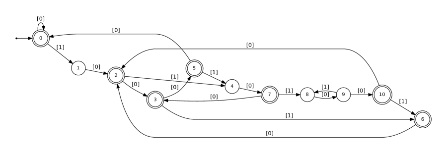
Figure 29: Automaton accepting orders of abelian cubes in $\bf f$

Theorem 63 has the following interesting corollary.

Corollary 69.

Let $h:\{0,1\}^{*}\rightarrow\Delta^{*}$ be an arbitrary morphism such that $h(01)\not=\epsilon$. Then $h({\bf f})$ is an infinite Fibonacci-automatic word.

Proof.

From Theorem 63 we see that there is a predicate $\operatorname{ZC}(n,n^{\prime})$ which is true if $n^{\prime}=|{\bf f}[0..n-1]|_{0}$ and false otherwise, and this predicate can be implemented as a finite automaton taking the inputs $n$ and $n^{\prime}$ in Fibonacci representation.

Suppose $h(0)=w$ and $h(1)=x$. Now, to show that h(f) is Fibonacci-automatic, it suffices to show that, for each letter $a\in\Delta$, the language of “fibers”

$$L_{a}=\{(n)_{F}:(h({\bf f}))[n]=a\}$$

is regular.

To see this, we write a predicate for the $n$ in the definition of $L_{a}$, namely

$$\exists q\ \exists r_{0}\ \exists r_{1}\ \exists m\ (q\leq n<q+|h({\bf f}[m])|)\ \wedge\ \operatorname{ZC}(m,r_{0})\ \wedge\ (r_{0}+r_{1}=m)\wedge\\ (r_{0}|w|+r_{1}|x|=q)\ \wedge\ (({\bf f}[m]=0\ \wedge\ w[n-q]=a)\ \vee\ ({\bf f}[m]=1\ \wedge\ x[n-q]=a)).$$

Notice that the predicate looks like it uses multiplication, but this multiplication can be replaced by repeated addition since $|w|$ and $|x|$ are constants here.

Unpacking this predicate we see that it asserts the existence of $m$, $q$, $r_{0}$, and $r_{1}$ having the meaning that

• the $n$’th symbol of h(f) lies inside the block $h({\bf f}[m])$ and is in fact the $(n-q)$’th symbol in the block (with the first symbol being symbol 0)

• ${\bf f}[0..m-1]$ has $r_{0}$ 0’s in it

• ${\bf f}[0..m-1]$ has $r_{1}$ 1’s in it

• the length of $h({\bf f}[0..m-1])$ is $q$

Since everything in this predicate is in the logical theory $({\mathbb{N}},+,<,F)$ where $F$ is the predicate for the Fibonacci word, the language $L_{a}$ is regular. ∎

Remark 70.

Notice that everything in this proof goes through for other numeration systems, provided the original word has the property that the Parikh vector of the prefix of length $n$ is synchronized.

10 Details about our implementation

Our program is written in JAVA, and was developed using the Eclipse development environment. We used the dk.brics.automaton package, developed by Anders Møller at Aarhus University, for automaton minimization. Maple 15 was used to compute characteristic polynomials. The GraphViz package was used to display automata.

Our program consists of about 2000 lines of code. We used Hopcroft’s algorithm for DFA minimization.

A user interface is provided to enter queries in a language very similar to the language of first-order logic. The intermediate and final result of a query are all automata. At every intermediate step, we chose to do minimization and determinization, if necessary. Each automaton accepts tuples of integers in the numeration system of choice. The built-in numeration systems are ordinary base-$k$ representations and Fibonacci base. However, the program can be used with any numeration system for which an automaton for addition and ordering can be provided. These numeration system-specific automata can be declared in text files following a simple syntax. For the automaton resulting from a query it is always guaranteed that if a tuple $t$ of integers is accepted, all tuples obtained from $t$ by addition or truncation of leading zeros are also accepted. In Fibonacci representation, we make sure that the accepting integers do not contain consecutive $1$’s.

The program was tested against hundreds of different test cases varying in simplicity from the most basic test cases testing only one feature at a time, to more comprehensive ones with many alternating quantifiers. We also used known facts about automatic sequences and Fibonacci word in the literature to test our program, and in all those cases we were able to get the same result as in the literature. In a few cases, we were even able to find small errors in those earlier results.

The source code and manual will soon be available for free download.

11 Acknowledgments

We thank Kalle Saari for bringing our attention to the small error in [39]. We thank Narad Rampersad and Michel Rigo for useful suggestions.

Eric Rowland thought about the proof of Theorem 54 with us in 2010, and was able to prove at that time that the word $1213121512131218\cdots$ avoids additive squares. We acknowledge his prior work on this problem and thank him for allowing us to quote it here.

References

- [1] C. Ahlbach, J. Usatine, C. Frougny, and N. Pippenger. Efficient algorithms for Zeckendorf arithmetic. Fibonacci Quart. 51 (2013), 249–256.
- [2] J.-P. Allouche, N. Rampersad, and J. Shallit. Periodicity, repetitions, and orbits of an automatic sequence. Theoret. Comput. Sci. 410 (2009), 2795–2803.
- [3] J.-P. Allouche, K. Scheicher, and R. F. Tichy. Regular maps in generalized number systems. Math. Slovaca 50 (2000), 41–58.
- [4] J.-P. Allouche and J. Shallit. Automatic Sequences: Theory, Applications, Generalizations. Cambridge University Press, 2003.
- [5] J. Berstel. Mots de Fibonacci. Séminaire d’Informatique Théorique, LITP 6-7 (1980–81), 57–78.
- [6] J. Berstel. Fonctions rationnelles et addition. In M. Blab, editor, Théorie des Langages, École de printemps d’informatique théorique, pp. 177–183. LITP, 1982.
- [7] J. Berstel. Fibonacci words—a survey. In G. Rozenberg and A. Salomaa, editors, The Book of L, pp. 13–27. Springer-Verlag, 1986.
- [8] J. Berstel and C. Reutenauer. Noncommutative Rational Series with Applications, Vol. 137 of Encylopedia of Mathematics and Its Applications. Cambridge University Press, 2011.
- [9] B. Bischoff, J. D. Currie, and D. Nowotka. Unary patterns with involution. Internat. J. Found. Comp. Sci. 23 (2012), 1641–1652.
- [10] B. Bischoff and D. Nowotka. Pattern avoidability with involution. In WORDS 2011, pp. 65–70, 2011. Available at http://rvg.web.cse.unsw.edu.au/eptcs/content.cgi?WORDS2011.
- [11] A. Blondin Massé, S. Brlek, A. Garon, and S. Labbé. Two infinite families of polyominoes that tile the plane by translation in two distinct ways. Theoret. Comput. Sci. 412 (2011), 4778–4786.
- [12] A. Blondin Massé, S. Brlek, S. Labbé, and M. Mendès France. Fibonacci snowflakes. Ann. Sci. Math. Québec 35 (2011), 141–152.
- [13] A. Blondin Massé, S. Brlek, S. Labbé, and M. Mendès France. Complexity of the Fibonacci snowflake. Fractals 20 (2012), 257–260.
- [14] J.-P. Borel and F. Laubie. Quelques mots sur la droite projective réelle. J. Théorie Nombres Bordeaux 5 (1993), 23–51.
- [15] T. C. Brown and A. R. Freedman. Arithmetic progressions in lacunary sets. Rocky Mountain J. Math. 17 (1987), 587–596.
- [16] V. Bruyère and G. Hansel. Bertrand numeration systems and recognizability. Theoret. Comput. Sci. 181 (1997), 17–43.
- [17] V. Bruyère, G. Hansel, C. Michaux, and R. Villemaire. Logic and -recognizable sets of integers. Bull. Belgian Math. Soc. 1 (1994), 191–238. Corrigendum, Bull. Belg. Math. Soc. 1 (1994), 577.
- [18] J. R. Büchi. Weak secord-order arithmetic and finite automata. Zeitschrift für mathematische Logik und Grundlagen der Mathematik 6 (1960), 66–92. Reprinted in S. Mac Lane and D. Siefkes, eds., The Collected Works of J. Richard Büchi, Springer-Verlag, 1990, pp. 398–424.
- [19] L. Carlitz. Fibonacci representations. Fibonacci Quart. 6 (1968), 193–220.
- [20] A. Carpi and V. D’Alonzo. On the repetitivity index of infinite words. Internat. J. Algebra Comput. 19 (2009), 145–158.
- [21] A. Carpi and V. D’Alonzo. On factors of synchronized sequences. Theoret. Comput. Sci. 411 (2010), 3932–3937.
- [22] A. Carpi and C. Maggi. On synchronized sequences and their separators. RAIRO Inform. Théor. App. 35 (2001), 513–524.
- [23] J. Cassaigne. Sequences with grouped factors. In Developments in Language Theory III, pp. 211–222. Aristotle University of Thessaloniki, 1998.
- [24] J. Cassaigne, J. Currie, L. Schaeffer, and J. Shallit. Avoiding three consecutive blocks of the same size and same sum. Preprint, 2013.
- [25] E. Charlier, N. Rampersad, and J. Shallit. Enumeration and decidable properties of automatic sequences. Internat. J. Found. Comp. Sci. 23 (2012), 1035–1066.
- [26] M. Christou, M. Crochemore, and C. S. Iliopoulos. Quasiperiodicities in Fibonacci strings. To appear in Ars Combinatoria. Preprint available at http://arxiv.org/abs/1201.6162, 2012.
- [27] W.-F. Chuan. Symmetric Fibonacci words. Fibonacci Quart. 31 (1993), 251–255.
- [28] A. Cobham. Uniform tag sequences. Math. Systems Theory 6 (1972), 164–192.
- [29] M. Crochemore. An optimal algorithm for computing the repetitions in a word. Inform. Process. Lett. 12 (1981), 244–250.
- [30] L. J. Cummings, D. Moore, and J. Karhumäki. Borders of Fibonacci strings. J. Combin. Math. Combin. Comput. 20 (1996), 81–87.
- [31] L. J. Cummings and W. F. Smyth. Weak repetitions in strings. J. Combin. Math. Combin. Comput. 24 (1997), 33–48.
- [32] J. D. Currie. Pattern avoidance with involution. Available at http://arxiv.org/abs/1105.2849, 2011.
- [33] J. D. Currie, N. Rampersad, and K. Saari. Suffix conjugates for a class of morphic subshifts. In J. Karhumäki, A. Lepistö, and L. Zamboni, editors, WORDS 2013, Vol. 8079 of Lecture Notes in Computer Science, pp. 95–106. Springer-Verlag, 2013.
- [34] J. D. Currie and K. Saari. Least periods of factors of infinite words. RAIRO Inform. Théor. App. 43 (2009), 165–178.
- [35] A. de Luca. A combinatorial property of the Fibonacci words. Inform. Process. Lett. 12 (1981), 193–195.
- [36] X. Droubay. Palindromes in the Fibonacci word. Inform. Process. Lett. 55 (1995), 217–221.
- [37] D. D. A. Epple and J. Siefken. Collapse: a Fibonacci and Sturmian game. Available at http://www.siefkenj.com/tmp/Fibonacci-4.pdf, 2014.
- [38] A. S. Fraenkel. Systems of numeration. Amer. Math. Monthly 92 (1985), 105–114.
- [39] A. S. Fraenkel and J. Simpson. The exact number of squares in Fibonacci words. Theoret. Comput. Sci. 218 (1999), 95–106.
- [40] C. Frougny. Linear numeration systems of order two. Inform. Comput. 77 (1988), 233–259.
- [41] C. Frougny. Fibonacci representations and finite automata. IEEE Trans. Inform. Theory 37 (1991), 393–399.
- [42] C. Frougny. Representations of numbers and finite automata. Math. Systems Theory 25 (1992), 37–60.
- [43] C. Frougny and B. Solomyak. On representation of integers in linear numeration systems. In M. Pollicott and K. Schmidt, editors, Ergodic Theory of Actions (Warwick, 1993–1994), Vol. 228 of London Mathematical Society Lecture Note Series, pp. 345–368. Cambridge University Press, 1996.
- [44] D. Goc, D. Henshall, and J. Shallit. Automatic theorem-proving in combinatorics on words. In N. Moreira and R. Reis, editors, CIAA 2012, Vol. 7381 of Lecture Notes in Computer Science, pp. 180–191. Springer-Verlag, 2012.
- [45] D. Goc, H. Mousavi, and J. Shallit. On the number of unbordered factors. In A.-H. Dediu, C. Martin-Vide, and B. Truthe, editors, LATA 2013, Vol. 7810 of Lecture Notes in Computer Science, pp. 299–310. Springer-Verlag, 2013.
- [46] D. Goc, K. Saari, and J. Shallit. Primitive words and Lyndon words in automatic and linearly recurrent sequences. In A.-H. Dediu, C. Martin-Vide, and B. Truthe, editors, LATA 2013, Vol. 7810 of Lecture Notes in Computer Science, pp. 311–322. Springer-Verlag, 2013.
- [47] D. Goc, L. Schaeffer, and J. Shallit. The subword complexity of -automatic sequences is -synchronized. In M.-P. Béal and O. Carton, editors, DLT 2013, Vol. 7907 of Lecture Notes in Computer Science, pp. 252–263. Springer-Verlag, 2013.
- [48] M. Guay-Paquet and J. Shallit. Avoiding squares and overlaps over the natural numbers. Discrete Math. 309 (2009), 6245–6254.
- [49] L. Halbeisen and N. Hungerbühler. An application of Van der Waerden’s theorem in additive number theory. INTEGERS: Elect. J. of Combin. Number Theory 0 (2000), #A7. http://www.integers-ejcnt.org/vol0.html.
- [50] C. Holton and L. Q. Zamboni. Directed graphs and substitutions. Theory Comput. Systems 34 (2001), 545–564.
- [51] S. Homer and A. L. Selman. Computability and Complexity Theory. Springer-Verlag, 2nd edition, 2011.
- [52] C. S. Iliopoulos, D. Moore, and W. F. Smyth. A characterization of the squares in a Fibonacci string. Theoret. Comput. Sci. 172 (1997), 281–291.
- [53] J. Karhumäki. On cube-free -words generated by binary morphisms. Disc. Appl. Math. 5 (1983), 279–297.
- [54] R. Kolpakov and G. Kucherov. On maximal repetitions in words. In G. Ciobanu and G. Păun, editors, Fundamentals of Computation Theory: FCT ’99, Vol. 1684 of Lecture Notes in Computer Science, pp. 374–385. Springer-Verlag, 1999.
- [55] C. G. Lekkerkerker. Voorstelling van natuurlijke getallen door een som van getallen van Fibonacci. Simon Stevin 29 (1952), 190–195.
- [56] F. Mignosi and G. Pirillo. Repetitions in the Fibonacci infinite word. RAIRO Inform. Théor. App. 26 (1992), 199–204.
- [57] A. Monnerot-Dumaine. The Fibonacci word fractal. Published electronically at http://hal.archives-ouvertes.fr/hal-00367972/fr/, 2009.
- [58] M. Morse and G. A. Hedlund. Symbolic dynamics II. Sturmian trajectories. Amer. J. Math. 62 (1940), 1–42.
- [59] A. Ostrowski. Bemerkungen zur Theorie der Diophantischen Approximationen. Abh. Math. Sem. Hamburg 1 (1922), 77–98,250–251. Reprinted in Collected Mathematical Papers, Vol. 3, pp. 57–80.
- [60] G. Pirillo. Fibonacci numbers and words. Discrete Math. 173 (1997), 197–207.
- [61] G. Pirillo and S. Varricchio. On uniformly repetitive semigroups. Semigroup Forum 49 (1994), 125–129.
- [62] M. Presburger. Über die Volständigkeit eines gewissen Systems der Arithmetik ganzer Zahlen, in welchem die Addition als einzige Operation hervortritt. In Sparawozdanie z I Kongresu matematyków krajów slowianskich, pp. 92–101, 395. Warsaw, 1929.
- [63] M. Presburger. On the completeness of a certain system of arithmetic of whole numbers in which addition occurs as the only operation. Hist. Phil. Logic 12 (1991), 225–233.
- [64] N. Rampersad and J. Shallit. Words avoiding reversed subwords. J. Combin. Math. Combin. Comput. 54 (2005), 157–164.
- [65] M. Rao. On some generalizations of abelian power avoidability. Preprint, 2013.
- [66] G. Rote. Sequences with subword complexity . J. Number Theory 46 (1994), 196–213.
- [67] K. Saari. Periods of factors of the Fibonacci word. In WORDS 07, 2007.
- [68] K. Saari. Lyndon words and Fibonacci numbers. J. Combin. Theory. Ser. A 121 (2014), 34–44.
- [69] L. Schaeffer. Deciding properties of automatic sequences. Master’s thesis, University of Waterloo, 2013.
- [70] L. Schaeffer and J. Shallit. The critical exponent is computable for automatic sequences. Internat. J. Found. Comp. Sci. 23 (2012), 1611–1626.
- [71] P. Séébold. Propriétés combinatoires des mots infinis engendrés par certains morphismes (Thèse de cycle). PhD thesis, Université P. et M. Curie, Institut de Programmation, Paris, 1985.
- [72] J. O. Shallit. A generalization of automatic sequences. Theoret. Comput. Sci. 61 (1988), 1–16.
- [73] J. Shallit. Decidability and enumeration for automatic sequences: a survey. In A. A. Bulatov and A. M. Shur, editors, CSR 2013, Vol. 7913 of Lecture Notes in Computer Science, pp. 49–63. Springer-Verlag, 2013.
- [74] E. Zeckendorf. Représentation des nombres naturels par une somme de nombres de Fibonacci ou de nombres Lucas. Bull. Soc. Roy. Liège 41 (1972), 179–182.