Hierarchy and size distribution function of star formation regions in the spiral galaxy NGC 628

Abstract

Hierarchical structures and size distribution of star formation regions in the nearby spiral galaxy NGC 628 are studied over a range of scale from 50 to 1000 pc using optical images obtained with 1.5 m telescope of the Maidanak Observatory. We found hierarchically structured concentrations of star formation regions in the galaxy, smaller regions with a higher surface brightness are located inside larger complexes having a lower surface brightness. We illustrate this hierarchy by dendrogram, or structure tree of the detected star formation regions, which demonstrates that most of these regions are combined into larger structures over several levels. We found three characteristic sizes of young star groups: $\approx 65$ pc (OB associations), $\approx 240$ pc (stellar aggregates) and $\approx 600$ pc (star complexes). The cumulative size distribution function of star formation regions is found to be a power law with a slope of approximately $-1.5$ on scales appropriate to diameters of associations, aggregates and complexes. This slope is close to the slope which was found earlier by B. Elmegreen et al. for star formation regions in the galaxy on scales from 2 to 100 pc.

1 Introduction

As is known, such physical processes as gravitational collapse and turbulence compression play a key role in creation and evolution of star formation regions over the wide range of scales, from star complexes over OB associations down to compact embedded clusters and to clumps of young stars inside them. These stellar systems form a continuous hierarchy of structures for all these scales (Efremov, 1995; Efremov & Elmegreen, 1998; Elmegreen et al., 2000; Elmegreen, 2002, 2006, 2011). It is suggested that the hierarchy extends up to 1 kpc (Efremov, Ivanov & Nikolov, 1987; Elmegreen & Efremov, 1996; Zhang, Fall & Whitmore, 2001).

Efremov et al. (1987) and Ivanov (1991) described at least three categories of hierarchical star groups on the largest levels: OB associations with a length scale $\approx 80$ pc, stellar aggregates with a length scale $\approx 250$ pc and star complexes with diameters $\approx 600$ pc. H i/H₂ superclouds are ancestors of star complexes; OB associations are formed from giant molecular clouds (Efremov, 1989, 1995; Efremov & Elmegreen, 1998; Elmegreen, 1994; Elmegreen & Efremov, 1996; Elmegreen, 2009; Odekon, 2008; de la Fuente Marcos & de la Fuente Marcos, 2009). Sizes and clustering of these structures have been studied for many nearby spiral and irregular galaxies (Bastian et al., 2005; Bianchi et al., 2012; Battinelli, 1991; Battinelli, Efremov & Magnier, 1996; Borissova et al., 2004; Bresolin, Kennicutt & Stetson, 1996, 1998; Bruevich, Gusev & Guslyakova, 2011; Elmegreen & Elmegreen, 2001; Feitzinger & Braunsfurth, 1984; Gouliermis et al., 2010; Gusev, 2002; Harris & Zaritsky, 1999; Magnier et al., 1993; Pietrzyński et al., 2001, 2005; Sánchez et al., 2010; Wilson, 1991, 1992). Power-law power spectra of optical light in galaxies suggest the same maximum scale, possibly including the ambient galactic Jeans length (Elmegreen, Elmegreen & Leitner, 2003a, b). If the ambient Jeans length is the largest scale, then a combination of gravitational and turbulent fragmentations can drive the whole process. Observed star formation rates in galaxies can follow from such turbulent structures (Krumholz & McKee, 2005).

Hierarchical clustering disappears with age as stars mix. The densest regions have the shortest mixing times and lose their substructures first. Nevertheless, very young clusters have a similar pattern of subclustering, suggesting that this structure continues down to individual stars (Brandeker, Jayawardhana & Najita, 2003; Dahm & Simon, 2005; Heydari-Malayeri et al., 2001; Kumar, Kamath & Davis, 2004; Oey et al., 2005; Sánchez-Monge et al., 2013).

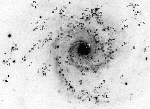
Figure 1: $B$ image of NGC 628 and positions of the galaxy’s star formation regions (crosses). The numbers of the star formation regions from Table 3 are indicated. The image size is $8.26\times 6.00$ arcmin. North is upward and east is to the left.

Table 1: Basic parameters of NGC 628.

Parameter	Value
Type	Sc
RA (J2000.0)	01h36m41.81s
DEC (J2000.0)	+15$\degr$47$\arcmin$00.3$\arcsec$
Total apparent $B$ magnitude ($B_{t}$)	9.70 mag
Absolute $B$ magnitude ($M_{B}$)a	-20.72 mag
Inclination ($i$)	$7\degr$
Position angle (PA)	$25\degr$
Apparent corrected radius ($R_{25}$)b	5.23 arcmin
Apparent corrected radius ($R_{25}$)b	10.96 kpc
Distance ($D$)	7.2 Mpc

^a Absolute magnitude of a galaxy corrected for Galactic extinction and inclination effect.

^b Isophotal radius (25 mag arcsec^-2 in the $B$-band) corrected for Galactic extinction and absorption due to the inclination of NGC 628.

The interstellar matter also shows a hierarchical structure from the largest giant molecular clouds down to individual clumps and cores. The complex hierarchical structure of the interstellar matter is shaped by supersonic turbulence (Ballesteros-Paredes et al., 2007). The scaling relations observed in molecular clouds (Larson, 1981) can be explained by the effect of turbulence, where energy is injected at largest scales and cascades down to the smallest scales, creating eddies and leading to a hierarchical structure on all scales (Elmegreen et al., 2006). It is believed that turbulence plays a major role in star formation; it creates density enhancements that become gravitationally unstable and collapse to form stars (Elmegreen et al., 2006). The spatial distribution of young stars and stellar groups on wide length scales probably reflects this process.

The purpose of this paper is to study size distribution and hierarchical structures of star formation regions in nearby face-on spiral galaxy NGC 628 (Fig. 1), based on our own observations in the $U$, $B$, and $V$ passbands. This galaxy is an excellent example of a galaxy with numerous star formation regions observed at different length scales. We use the term ’star formation regions’, which includes young star complexes, OB associations, H ii regions, i.e. all young stellar groups regardless of their sizes.

Hodge (1976) identified 730 H ii regions in the galaxy. Ivanov et al. (1992) estimated sizes and magnitudes of 147 young stellar associations and aggregates in NGC 628 and discussed briefly hierarchical structures at the scales from 50 to 800 pc. Larsen (1999) studied 38 young star clusters with an effective diameters from 2 to 90 pc. Bruevich et al. (2007) obtained magnitudes, colours and sizes of 186 star formation regions based on the list of H ii regions from Belley & Roy (1992).

Elmegreen et al. (2006) studied distributions of size and luminosity of star formation regions over a range of scales from 2 to 110 pc using progressively blurred versions of blue optical and H$\alpha$ images from the Hubble Space Telescope (HST). They counted and measured features in each blurred image using SExtractor program and found that the cumulative size distribution satisfies a power law with a slope of approximately from –1.8 to –1.5 on all studied scales.

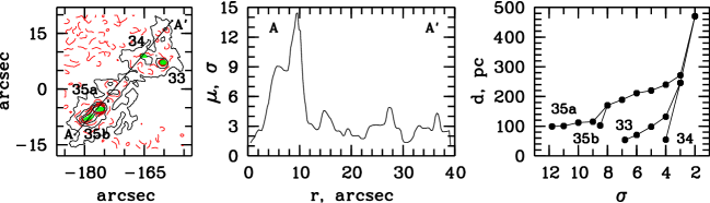
Figure 2: Left panel: contour map of the vicinity of star formation regions Nos. 33-35. Grey areas correspond to the regions Nos. 33, 34, 35a, and 35b within their half-maximum brightness level. Red dashed contour levels correspond to the levels of $\sigma$, $3\sigma$, $5\sigma$, $7\sigma$, and $9\sigma$, black solid contour levels correspond to the levels of $2\sigma$, $4\sigma$, $6\sigma$, $8\sigma$, and $10\sigma$ above the average brightness level of background. Position of profile A–A’ is shown. Central panel: photometric profile A–A’. Surface brightness, $\mu$, is given in units of $\sigma$. Right panel: diameters of star formation regions Nos. 33-35 and their hierarchical structures measured at the different levels of surface brightness in units of $\sigma$.

The fundamental parameters of NGC 628 are presented in Table 1. We take the distance to NGC 628, obtained in Sharina, Karachentsev & Tikhonov (1996) and van Dyk, Li & Filippenko (2006). We used the position angle and the inclination of the galactic disc, derived by Sakhibov & Smirnov (2004). Other parameters were taken from the LEDA data base (Paturel et al., 2003). We adopt the Hubble constant $H_{0}=75$ km s^-1Mpc^-1 in the paper. With the assumed distance to NGC 628, we estimate a linear scale of 34.9 pc arcsec^-1.

Observations and reduction stages of $UBVRI$ images for NGC 628 have already been published in Bruevich et al. (2007). The reduction of the photometric data was carried out using standard techniques, with the European Southern Observatory Munich Image Data Analysis System (eso-midas).

2 Identification and size estimations of star formation regions

In Bruevich et al. (2007), we have identified star formation regions in the galaxy with the list of H ii regions of Belley & Roy (1992), based on their H$\alpha$ spectrophotometric data. The list of Belley & Roy (1992) is still the most complete survey of H ii regions and their parameters in NGC 628. Note that our coordinate grid coincides with that of Kennicutt & Hodge (1980) and is systematically shifted with respect to that of Belley & Roy (1992). Altogether, we identified 127 of 132 star formation regions studied in Belley & Roy (1992). Three regions (Nos. 1, 2, and 96 in Belley & Roy, 1992) were outside the field of view of our images. Two star formation regions (Nos. 23 and 76) are missing in the list of Belley & Roy (1992). Belley & Roy (1992) did not distinguish between isolated star formation regions, with typical sizes about 60-70 pc, and compound multi-component regions, with typical sizes about 200 pc. We obtained images of the galaxy with better seeing than Belley & Roy (1992). As a result, we were able to resolve the compound star formation regions into components.

Firstly, we identified such subcomponents by eye. We selected the components, the maximal (central) brightness in which was at least 3 times higher than the brightness of surrounding background. Next, we fitted profiles of star formation regions using Gaussians. The components separation condition was that the full width at half-maximum (FWHM) of the region is less than the distance between centres of Gaussians. Numbers of these complexes in the first column of Table 3 contain additional letters: ’a’, ’b’, ’c’, and ’d’. Compound regions which do not satisfy this condition were classified as objects with observed, but unresolved, internal structure. In total, we identified 186 objects (Fig. 1).

In this paper we use the numbering order adopted in Bruevich et al. (2007). It coincides with the numbering order of Belley & Roy (1992) with the exception of the missed star formation regions.

We found that 146 regions from Table 3 have a star-like profile (see the last column in this table). Other 40 objects have a non-star-like (extended (diffuse) or multi-component) profile, i.e. these objects have an observed, but unresolved, internal structure.

We took the geometric mean of major and minor axes of a star formation region for the star formation region’s characteristic diameter $d$: $d=\sqrt{d_{max}\times d_{min}}$. We measured $d_{max}$ and $d_{min}$ from the radial $V$ profiles as the FWHM for regions having a star-like profile, or as the distance between points of maximum flux gradient for regions having non-star-like profiles. We adopted seeing for the uncertainty in the size measurements, which definitely exceeds all other errors. Obtained parameters of star formation regions are presented in Table 3.

3 Hierarchical structures of star formation regions

The simplest way to study hierarchical clustering is to identify structures of different hierarchical levels based on lower level surface brightness thresholds above the background level. The similar method was used by Gouliermis et al. (2010), who used the stellar density levels to study hierarchical stellar structures in the dwarf irregular galaxy NGC 6822. They identified hierarchical structures using density thresholds $1\sigma-5\sigma$ above the average background density level with step of $1\sigma$.

However, this direct way is not applicable for identification of hierarchical structures in NGC 628. The background level varies significantly in the galactic plane. The surface brightness of the background differs by several times inside spiral arms and in interarm regions.

Therefore we modified the technique of Gouliermis et al. (2010). Identification and size estimation of 186 star formation regions at the highest hierarchical level (Level 1) were done using their half-maximum brightness levels, independent of background levels (see Section 2). Additionally, we fitted the profiles of star formation regions along their minor and major axes using Gaussians. To identify structures of Level 2 and lower, we measured the background surface brightness in the $V$ passband in the vicinity of every group of star formation regions of Level 1.

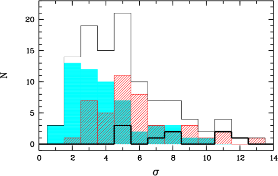
Figure 3: Distribution histogram of star formation regions of Levels 2-5 by the level of maximum brightness decrease. Brightness is given in units of $\sigma$. Grey histogram is the distribution of star formation regions of the lowest hierarchical level. Shaded histogram is the distribution of star formation regions of the first hierarchical level from the lowest one. Thick black histogram is the distribution of star formation regions of the second hierarchical level from the lowest one. See the text for details.

The selection of a threshold in units of $\sigma$ above the average brightness level of background for star formation regions of Level 2 was carried out based on two basic conditions: (i) it must be lower than the level of brightness of the appropriate star formation region of Level 1 and (ii) it must deviate more than 4 pixels (seeing of the $V$ image) from the fitting Gaussian of the profile of the star formation region at Level 1. The same conditions were applied to select the brightness level of every next lower level of the hierarchy. The exception was made for several resolved close binary star formation regions, such as 40a-40b, where the second condition is not applied. To identify star formation regions of lower hierarchical levels, we used lower levels of brightness.

To select surface brightness thresholds, we firstly analysed a typical light distribution in selected star formation regions and their vicinities. Example of such region, star formation regions Nos. 33-35, is given in Fig. 2.

Fig. 2 (central panel) shows that the surface brightness falls irregularly with distance from the knots of star formation: ’plateau-like’ areas with constant surface brightness alternate with areas of a sharp drop in brightness. At such sites, a fall in brightness usually exceeds $1\sigma$ value. At higher hierarchical levels, where the surface brightness is higher, absolute drop in brightness is larger than at lower levels of the hierarchy. As a result, diameters of star formation regions increase slowly with a decrease of brightness level within the same hierarchical level. Significant growth of the diameters is observed only at merger of two separate star formation regions into one common star formation region at the lower hierarchical level (Fig. 2).

We consider brightness in units of $\sigma$. So the brightness level, where the maximum brightness decrease is observed, is also measured in units of $\sigma$. Maximum brightness decrease corresponds to the minimum of first derivative of the brightness profile function (Fig. 2, central panel) in units of $\sigma$. After measuring the brightness level in units of $\sigma$ by the maximum brightness decrease, we determine size of star formation region with the isophots as described in Section 2.

We analysed all hierarchical structures in vicinities of star formation regions of Level 1 and determined which level of brightness corresponds to the level of maximum brightness decrease in them (Fig. 3).

Distribution of star formation regions of Levels 2-5 by the level of maximum brightness decrease shows two maxima at $3\sigma$ and $5\sigma$ (Fig. 3). Distribution of star formation regions of the lowest hierarchical level has a maximum at $2\sigma-3\sigma$, distribution of star formation regions of the first hierarchical level from the lowest one shows maxima at $3\sigma$ and $5\sigma-6\sigma$. Star formation regions of the second hierarchical level from the lowest one have characteristic levels of maximum brightness decrease of $5\sigma$, $8\sigma$, and $11\sigma$ (Fig. 3).

Analysis of the distribution of star formation regions by the level of maximum brightness decrease, in units of $\sigma$, has shown that neither arithmetic nor geometric sequences of the brightness levels are suitable to describe the hierarchical structures of star formation regions. When using a geometric sequence, we may miss some of the hierarchical levels. When using an arithmetic sequence, we lose some of the brightness levels because they do not satisfy the condition (ii) (Fig. 2). In this case, low hierarchical levels will correspond to arbitrary levels of brightness.

Analysis of the distribution showed that the best sequence of brightness levels is the Fibonacci sequence, $1\sigma$, $2\sigma$, $3\sigma$, $5\sigma$, $8\sigma$, as an intermediate sequence between arithmetic and geometric sequences.

Diameters of star formation regions of the lower hierarchical levels which have the maximum brightness decrease at the level of $4\sigma$ or $6\sigma-7\sigma$ are measured at the next lower surface brightness level of $3\sigma$ or $5\sigma$, respectively. Typically, the difference between diameters measured at the levels of $3\sigma$ and $4\sigma$, or $5\sigma$ and $6\sigma-7\sigma$ does not exceed 35-40 pc, a value of the seeing of the image (Fig. 2).

Thus, we used surface brightness thresholds of $8\sigma$, $5\sigma$, $3\sigma$ and $2\sigma$ above the average brightness level of background in the vicinity of star formation region. The threshold of $1\sigma$ was not used due to large fluctuations of background around many identified groups of star formation regions.

For each individual region, not every next lower brightness level satisfies the conditions adopted. Such brightness levels were missed. Furthermore, a full set of brightness levels from $8\sigma$ to $2\sigma$ above the background was used only for star formation regions Nos. 79a and 79b and hierarchical structures of a lower order related with them (Table 4). The lowest level of every hierarchical structure usually corresponds to the brightness level of $2\sigma$ or $3\sigma$ above the background (Fig. 3). As a result, the same hierarchical level may correspond to different levels of brightness.

Diameters of star formation regions at Levels 2 and lower were measured in the same manner as for star formation regions of Level 1: $d=\sqrt{d_{max}\times d_{min}}$, where $d_{min}$ and $d_{max}$ are diameters along the major and minor axes of star formation region.

Star formation regions obtained on different hierarchical levels, and their sizes are presented in Table 4. Some star formation regions of low hierarchical levels consist of one or several star-like cores (star formation regions of Level 1) and an extended halo. Such star formation regions are indicated by letter ’h’ in Table 4. A map of location of these objects in the galactic plane is shown in Fig. 4.

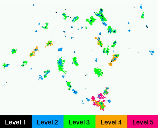
Figure 4: Map of star formation regions of different levels of the hierarchy. Regions of higher levels of the hierarchy are shaded darker than lower ones. The image size is $8.26\times 6.00$ arcmin. North is upward and east is to the left.

To illustrate the hierarchical structures we used so-called dendrograms. Dendrograms were introduced as ’structure trees’ for analysis of molecular cloud structures by Houlahan & Scalo (1992), refined by Rosolowsky et al. (2008), and used in Gouliermis et al. (2010) to study hierarchical stellar structures in the nearby dwarf galaxy NGC 6822. A dendrogram is constructed by cutting an image at different brightnesses and identifying connected areas, while keeping track of the connection to surface brighter smaller structures (on a higher level) and surface fainter larger structures (on the next lower level, which combines structures of the previous level).

The dendrogram for the star formation regions from Tables 3 and 4 is presented in Fig. 5. Unlike Gouliermis et al. (2010), we constructed the dendrogram using the ordinate axis in units of diameter. It better illustrates length scales of hierarchical structures. The combination of this dendrogram with the map of Fig. 4 illustrates graphically the hierarchical spatial distribution of star formation regions in NGC 628.

The dendrogram demonstrates that most star formation regions are combined into larger structures over, at least, 1-2 levels. We found only 12 separate associations without visible internal structure, which are out of hierarchical structures (Fig. 5). Most of them are located in interarm regions (Fig. 1). The largest ($d>1$ kpc) and the most populous (8-17 star formation regions of Level 1) structures are located in the ends of spiral arms. First of them (Nos. 75-80) is located near the corotation radius, which was obtained in Sakhibov & Smirnov (2004) based on a Fourier analysis of the spatial distribution of radial velocities of the gas in the disc of NGC 628. Largest and brightest in UV star complex of the galaxy was found here in Gusev, Egorov & Sakhibov (2014). Second structure (Nos. 120-127) is located in the nothern-western part of NGC 628, in the disturbed part of the spiral arm (Fig. 1).

As seen from the dendrogram, the numbering order does not reflect correctly the hierarchical structures. The numbering is violated for star formation regions Nos. 4-7 at Level 2, Nos. 85-89 at Level 4, and Nos. 97-109 at Level 4 (Table 4).

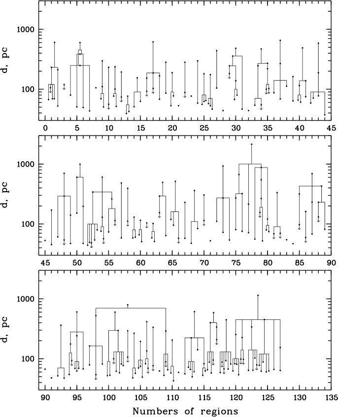
Figure 5: Dendrogram of star formation regions structures. The black dots indicate star formation regions from Tables 3, 4. Regions which are united into a hierarchical structure are connected by solid line. The numbering order might not strictly follow the order of hierarchical structures (see the text for details). The arrows down indicate star formation regions with an observed internal structure (star formation regions with a non-star-like profile).

4 Size distributions of star formation regions

In Fig. 6, we present size distribution histograms for three sets of star formation regions under study. The first set includes 297 regions of all hierarchical levels, the second set is a sample of 146 associations with a star-like profile, and the third set includes 111 regions of Level 2 and lower from Table 4. The second set unites the star formation regions without an observed internal structure; their subcomponents (if exist) have sizes $\leq 35-40$ pc. The third set includes only star formation regions with obvious internal structure; their subcomponents were detected and measured.

As seen from the figure, associations with a star-like profile have a narrow range of sizes, from 40 to 100 pc, with a few exceptions. The mean diameter of these star formation regions is equal to $66\pm 18$ pc. This is a typical size of OB associations. Star formation regions with extended profile have, on average, slightly larger sizes, $\sim 100$ pc. As a result, the size distribution of star formation regions of Level 1 with both star-like and extended profiles is displaced a little toward the larger sizes (see Fig. 6 and Table 2).

Star formation regions of lower levels clearly show a bimodal size distribution. Two maxima at $\approx 250$ and $\approx 600$ pc are observed (Fig. 6). The first smoothed peak corresponds to a characteristic size of stellar aggregates by classification of Efremov et al. (1987), and the second peak is located on diameters, which are typical for star complexes.

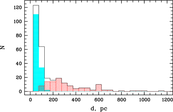
Figure 6: Number distribution histograms of all star formation regions from Tables 3 and 4, star formation regions of Level 1 with a star-like profile (grey histogram), and star formation regions of Levels 2 and lower (shaded histogram).

Table 2: Diameters of star formation regions.

Star formation	$d^{a}$	$d^{b}$
regions	(pc)	(pc)
Associationsc	$66\pm 18$	64
Associationsd	$72\pm 26$	66
Aggregates	$240\pm 90$	234
Complexes	$583\pm 84$	601

^a Mean diameter. ^b Diameter obtained from best fitting Gaussian.

^c Associations with a star-like profile (146 objects).

^d All associations from Table 3 (186 objects).

We also fitted size distributions of studied sets of star formation regions using Gaussians. To fit the size distribution for the set of 111 complex star formation regions, we used a combination of two Gaussians. It was found that all sets of star formation regions have size distributions close to the Gaussian distribution. Diameters obtained from the best-fit Gaussians are almost the same as the mean diameters for all sets of star formation regions (Table 2).

Following Elmegreen et al. (2006), we constrained the cumulative size distribution function in the form $N(d>D)\propto D^{\gamma}$, where $N$ is the integrated number of objects that have a diameter $d$ greater than some diameter $D$ (Fig. 7).

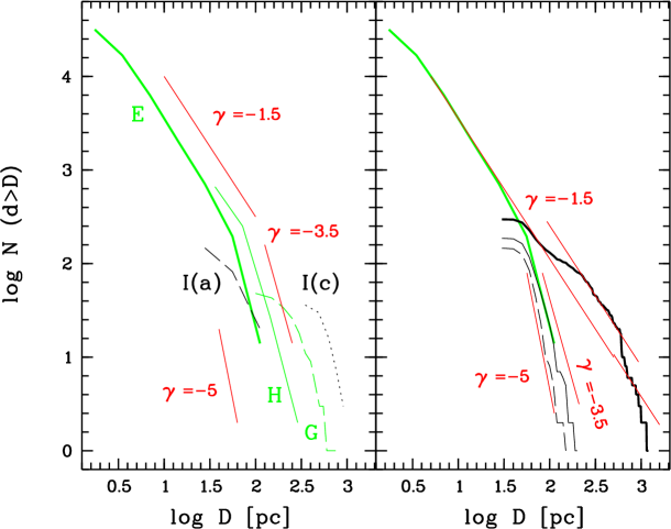
Figure 7: Left panel: cumulative size distribution functions for regions of Elmegreen et al. (2006) (E; grey thick solid curve), H ii regions of Hodge (1976) (H; grey thin solid curve), associations (I(a); black dashed curve) and complexes (I(c); black dotted curve) of Ivanov et al. (1992), large star formation regions in the spiral arms of the galaxy (G; grey thin dashed curve) from Gusev et al. (2014). Right panel: cumulative size distribution functions for regions of Elmegreen et al. (2006) (grey thick solid curve), 146 star formation regions with a star-like profile from Table 3 (black dashed curve), 186 star formation regions from Table 3 (black solid curve), and 297 star formation regions from Tables 3 and 4 (black thick curve). Dark thin solid straight lines in both panels represent slopes $\gamma$ = –1.5, –3.5 and –5 of the size distribution function. See the text for details.

Detailed exploration of the size distribution of objects in NGC 628 was made in Elmegreen et al. (2006) in the range of scales from 2 to 110 pc based on HST images. For regions in the central part of the galaxy brighter than the $3\sigma$ noise limits in $B$ and $V$ images, Elmegreen et al. (2006) found that the cumulative size distribution obeys a power law, with a slope $\gamma\approx-1.5$ in the range from 2 to 55 pc. The similar slope of the cumulative size distribution function was found for OB associations from the list of Ivanov et al. (1992) in the range from 30 to 110 pc. The size distribution of larger objects, H ii regions studied by Hodge (1976), satisfies a power law with a slope $\gamma\approx-3.5$ in the range from 100 to 300 pc. The size distribution of large star formation regions (in the range from 300 to 600 pc) in spiral arms of NGC 628 obtained in Gusev et al. (2014) shows a slope $\gamma\approx-4.5$. The size distribution of complexes from Ivanov et al. (1992) gives $\gamma=-4.1$ in the range from 500 to 1000 pc (Fig. 7).

Summarizing the results of the size distribution obtained previously, we can conclude that the size distributions of star formation regions with a diameter of $\leq 100$ pc satisfy a power law with $\gamma\approx-1.5$. The distribution of larger star formation regions obeys a power law with $\gamma$ between $\approx-5$ and $\approx-3.5$.

In Fig. 7 (right panel) we present size distribution functions constructed for three sets of star formation regions. The first set includes 297 regions of all hierarchical levels, the second set is a sample of 186 star formation regions of Level 1, and the third set includes 146 regions of Level 1 with star-like profile.

Size distribution of 146 star formation regions with a star-like profile, beginning with $d\approx 50$ pc, obeys a power law with a slope $\gamma\approx-5$. Size distribution of all 186 star formation regions of Level 1 satisfies a power law with a slope $-4\leq\gamma\leq-3.5$ in the range from 50 to 170 pc. It repeats the distribution of H ii regions of Hodge (1976) with a displacement $\log D\approx 0.2$ (Fig. 7). In general, the size distribution of star formation regions of Level 1 has slopes between –5 and –3.5, such as size distributions of previously studied star formation regions of a single level of hierarchy (Fig. 7).

Note, that the end of the size distribution curve for regions of Elmegreen et al. (2006) coincides with the beginning of the size distribution curve for our 186 star formation regions of Level 1 (Fig. 7). Given that the area studied in Elmegreen et al. (2006) occupies $\sim 70\%$ of the area of NGC 628, which is studied in this paper, we can conclude that (i) the number of H ii regions identified in Belley & Roy (1992) is smaller than the numbers of regions found by Elmegreen et al. (2006) using SExtractor, and, that is more important, (ii) our measurements of sizes of star formation regions using photometric profiles are in a good agreement with measurements of Elmegreen et al. (2006).

More interesting behaviour is observed for the curve of size distribution of star formation regions of all hierarchical levels. It continues the size distribution curve for regions of Elmegreen et al. (2006) at $d=30-40$ pc and has the same slope $\approx-1.5$ in the range from 45 to 85 pc – diameters of OB associations. Flatter slope, $\gamma>-1$, is observed in the range from $\approx 90$ to $\approx 180$ pc for regions of Level 1 with an extended profile and for the smallest regions of Level 2. Size distribution of star formation regions, which are classified as stellar aggregates and complexes, obeys a power law with $\gamma=-1.5$ very well (see the distribution curve in the range from 190 to 600 pc in Fig. 7). Largest hierarchical structures with $d=0.65-0.9$ kpc are also distributed by sizes by a power law with $\gamma\sim-1.5$ (Fig. 7).

Thus, the size distribution of star formation regions of all hierarchical levels continues the size distribution function for regions of Elmegreen et al. (2006) towards the larger sizes with the same slope $\approx-1.5$.

5 Discussion

The modern theory of star formation explains an existence of OB associations and star complexes, which are associated by unity of an origin with hydrogen superclouds and giant molecular clouds, respectively (Elmegreen & Efremov, 1996; Efremov & Elmegreen, 1998). Structures of H₂ on the intermediate scale length are unknown. However, such intermediate young stellar structures are observed in galaxies. These are stellar aggregates with diameters $\sim 200-300$ pc.

Our Fig. 6 shows a bimodal size distribution of star formation regions of Level 2 and lower. Bimodal size distributions with a secondary peak at $d=150-300$ pc were found for ’associations’ in SMC (Battinelli, 1991), M31 (Magnier et al., 1993), NGC 2090, NGC 2541, NGC 3351, NGC 3621 and NGC 4548 (Bresolin et al., 1998), NGC 1058 and UGC 12732 (Battinelli et al., 2000), NGC 300 (Pietrzyński et al., 2001), NGC 3507 and NGC 4394 (Vicari et al., 2002), NGC 7793 (Pietrzyński et al., 2005). Pietrzyński et al. (2005) named such ’associations’ ’superassociations’.

Thus, the existence of stellar structures, ’aggregates’ or ’superassociations’, with a characteristic size 200–300 pc is confirmed by numerous obsevations in different galaxies. However, the question of origin of stellar aggregates is still open.

As we noted above, the size distribution of star formation regions of all hierarchical levels continues the size distribution of regions of Elmegreen et al. (2006) with the same slope $\approx-1.5$ for sizes from 45 pc to $\sim 0.9$ kpc. However, the function of size distribution deviates from a power law with the slope –1.5 at $d=90-180$ pc and $600-650$ pc (Fig. 7).

We believe that the flatter slope in the range of 90 to 180 pc is a result of significant number of star formation regions with a diameter of $\sim 100-150$ pc with an unresolved internal structure. Taking into account such undetected objects will shift the distribution curve upward along the ordinate axis at sizes smaller than or equal to diameters of these star formation regions.

Opposite situation is observed at $d=600-650$ pc. Largest structures with $d>600$ pc have a low boundary surface brightness. They are difficult for identification in spiral arms of grand design galaxy NGC 628 because of the significant variations of background level (see Section 4). Underestimation a number of star formation regions at lowest hierarchical levels leads to a drastic drop in the size distribution curve.

In spite of small statistics, largest star formation regions with $d\approx 0.65-0.9$ kpc are also distributed by size by a power law with $\gamma\sim-1.5$. It can be an additional argument in favor of the assumption of Efremov et al. (1987), Elmegreen & Efremov (1996) and Zhang et al. (2001), who adopted that the hierarchical structures extend to the scale of 1 kpc.

Taking into account the hierarchy of star formation regions is crucial for construction of the cumulative size distribution function. Neglecting the internal structure of star formation regions of higher hierarchical levels and underestimation of the number of star formation regions of lower hierarchical levels leads to a decrease or an increase of the slope of the size distribution function, respectively. To illustrate this, we compare size distributions of regions of Elmegreen et al. (2006), our star formation regions of all hierarchical levels, and our star formation regions of Level 1 with any profiles in the range of scale from 50 to 110 pc in Fig. 7.

On the scale of 200–600 pc, the characteristic sizes of stellar aggregates and complexes, the size distribution function has a constant slope. We believe that the sample of objects at different levels of hierarchy within this range of scale is complete.

The slope $\gamma$ of the cumulative size distribution function for star formation regions is of fundamental importance. It is associated with the fractal dimension of objects in the galaxy at different scales. Elmegreen et al. (2006) introduced the fractal of dimension $\mathcal{D}\$, where $\mathcal{D}\ =-\gamma$. Following Elmegreen et al. (2006), we believe that the size distribution of stellar groups suggests a fractal distribution of stellar positions projected on the disc of the galaxy, with a constant fractal dimension of $\mathcal{D}\ \approx 1.5$ in the wide range of length scales from 2 pc to 1 kpc. It is comparable to the fractal dimension of projected local interstellar clouds, $\mathcal{D}\ \approx 1.3$ (Falgarone, Phillips & Walker, 1991), and to the fractal dimension of H i ($\mathcal{D}\ =1.2-1.5$) in the M81 group of galaxies (Westpfahl et al., 1999).

6 Conclusions

We studied hierarchical structures and the size distribution of star formation regions in the spiral galaxy NGC 628 over a range of scale from 50 to 1000 pc based on size estimations of 297 star formation regions. Most star formation regions are combined into larger structures over several levels. We found three characteristic sizes of young star groups: OB associations with mean diameter $d=66\pm 18$ pc, stellar aggregates ($d=240\pm 90$ pc) and star complexes ($583\pm 84$ pc).

The cumulative size distribution function of star formation regions satisfies a power law with a slope of $-1.5$ at scales from 45 to 85 pc, from 190 to 600 pc, and from 650 pc to 900 pc, which are appropriate to the sizes of associations, aggregates and complexes. Together with the result of Elmegreen et al. (2006), who found the slope $-1.8\leq\gamma\leq-1.5$ for regions at scales from 2 to 100 pc, our result shows that the size distribution of young stellar structures in the galaxy obeys a power law with a constant slope of $\approx-1.5$ at all studied scales from $\approx 2$ pc to $\approx 1$ kpc.

Ignoring the hierarchical structures, i.e. using star formation regions of only one of hierarchical levels to examine the size distribution, gives slopes $-5\leq\gamma\leq-3$.

Appendix A Parameters and hierarchical structures of star formation regions

Table 3: Identification, offsets, and diameters of star formation regions.

ID	ID	N–Sb	E–Wb	$d$	Note		ID	ID	N–S	E–W	$d$	Note		ID	ID	N–S	E–W	$d$	Note
	(BR)a	(arcsec)	(arcsec)	(pc)				(BR)	(arcsec)	(arcsec)	(pc)				(BR)	(arcsec)	(arcsec)	(pc)
1a	3	+108.8	–40.3	65	stc		48	51	–29.1	–40.1	55			97	102	+17.8	+42.9	80	st
1b	3	+106.9	–38.5	105			49	52	–33.6	–48.9	45	st		98	103	+25.8	+33.8	55
1c	3	+104.2	–37.4	70	st		50	53	–32.8	–88.3	150	st		99	104	+30.4	+38.3	80	st
1d	3	+110.4	–36.6	70	st		51	54	–52.3	–78.5	45	st		100a	105	+21.0	+75.1	50	st
2	4	+98.4	–48.6	50	st		52a	55	–57.1	–126.2	45	st		100b	105	+18.9	+77.0	55	st
3	5	+109.0	–54.5	120			52b	55	–62.2	–122.7	50	st		101a	106	+27.2	+81.0	100
4	6	+112.2	–61.9	80	st		52c	55	–59.5	–121.7	50			101b	106	+28.2	+83.4	60	st
5	7	+119.7	–72.9	50	st		53a	56	–67.5	–129.4	55	st		102a	107	+30.6	+82.9	60	st
6	8	+119.2	–76.1	50	st		53b	56	–64.8	–127.0	80	st		102b	107	+31.7	+86.9	80	st
7	9	+112.8	–67.0	45	st		54a	57	–64.3	–135.8	75	st		102c	107	+34.9	+86.1	75	st
8	10	+132.8	–72.3	105	st		54b	57	–61.6	–136.3	55			103	108	+69.0	+129.8	105
9a	11	+75.5	–4.9	70	st		55	58	–72.0	–132.6	75	st		104a	109	+89.6	+127.7	50	st
9b	11	+76.0	–8.6	50	st		56	59	–76.6	–136.9	115			104b	109	+92.0	+127.7	55	st
10	12	+78.1	–18.7	55			57	60	–74.4	–149.9	60	st		105a	110	+78.6	+186.1	70	st
11a	13	+71.7	–31.3	75	st		58	61	–74.4	–77.9	110			105b	110	+81.1	+183.4	75	st
11b	13	+72.0	–28.9	50	st		59a	62	–91.0	–68.9	60	st		105c	110	+83.2	+182.9	50	st
12	14	+77.1	–51.5	75			59b	62	–91.5	–67.0	60	st		106a	111	+115.2	+170.3	80	st
13a	15	+124.0	–101.1	40	st		60a	63	–70.7	–3.3	65	st		106b	111	+116.8	+174.3	70
13b	15	+124.2	–99.3	40	st		60b	63	–68.6	–2.7	50	st		107	112	+139.4	+166.6	75
14	16	+145.8	–170.2	50	st		61	64	–72.6	–7.3	105			108	113	+141.0	+145.0	60	st
15	17	+149.3	–170.7	65	st		62a	65	–112.3	–9.4	60	st		109a	114	+37.8	+33.5	55	st
16	18	+88.3	–128.9	90			62b	65	–114.2	–8.6	50	st		109b	114	+41.6	+36.2	90
17	19	+77.3	–133.7	105			63	66	–107.8	–55.5	155			109c	114	+44.2	+33.0	65	st
18	20	+80.3	–141.9	70	st		64	67	–116.8	–57.7	65	st		110a	115	+56.8	+35.9	60	st
19	21	+88.8	–153.1	85	st		65a	68	–122.4	–42.2	120	st		110b	115	+56.0	+38.6	45	st
20a	22	+63.7	–164.6	55	st		65b	68	–125.4	–41.7	95	st		111	116	+54.4	+15.7	60	st
20b	22	+64.8	–161.4	75	st		66	69	–127.2	–37.4	60			112	117	+98.1	+18.6	55	st
21	24	+5.8	+9.5	55	st		67	70	–160.8	–15.8	60	st		113a	118	+96.5	+8.2	70	st
22	25	+0.2	–43.0	90			68	71	–145.6	–4.6	45	st		113b	118	+99.7	+8.2	65	st
23	26	+57.6	–48.6	75	st		69	72	–149.9	+1.3	85	st		113c	118	+101.3	+9.3	50	st
24	27	+46.1	–51.0	60	st		70	73	–28.8	+25.3	115			113d	118	+99.2	+11.4	60	st
25a	28	+50.9	–73.7	55	st		71	74	–48.3	+29.8	50	st		114	119	+105.0	+13.0	140	st
25b	28	+51.4	–69.9	60	st		72	75	–65.4	+45.0	110	st		115a	120	+112.2	+11.1	55	st
25c	28	+48.8	–71.3	65	st		73	77	–64.3	+36.5	70	st		115b	120	+112.2	+12.5	65	st
26a	29	+64.2	–76.6	55	st		74	78	–77.1	+34.3	55	st		116a	121	+64.8	+64.5	65	st
26b	29	+64.8	–73.4	55	st		75	79	–113.4	+59.7	80	st		116b	121	+66.1	+67.5	90	st
26c	29	+62.6	–73.7	45	st		76	80	–125.1	+52.5	75	st		116c	121	+66.9	+70.3	60	st
27	30	+4.5	–92.3	105	st		77	81	–136.6	+34.6	70	st		116d	121	+62.6	+70.3	95
28	31	+46.4	–115.8	45	st		78	82	–150.4	+16.7	55	st		117	122	+65.3	+82.3	210
29	32	+28.5	–118.5	180			79a	83	–160.0	+42.6	155			118a	123	+87.2	+49.5	60	st
30a	33	+25.0	–126.7	65	st		79b	83	–164.6	+43.9	50	st		118b	123	+88.5	+51.4	90
30b	33	+22.9	–124.6	80	st		80a	84	–156.6	+25.8	80	st		118c	123	+88.2	+55.4	70
31	34	+17.0	–133.1	45	st		80b	84	–158.4	+27.4	75	st		118d	123	+85.0	+56.7	95	st
32	35	+19.7	–153.1	45	st		81	85	–157.1	+66.9	70			119a	124	+90.1	+48.7	65	st
33	36	+6.9	–160.3	55	st		82	86	–151.8	+63.1	70			119b	124	+91.7	+46.9	80	st
34	37	+8.0	–165.7	55			83	87	–47.0	+73.0	55	st		120a	125	+104.2	+41.0	60	st
35a	38	–5.1	–176.1	100			84	88	–94.2	+121.8	45	st		120b	125	+105.3	+45.5	80	st
35b	38	–7.8	–179.3	100			85	89	–28.3	+73.5	95			120c	125	+104.2	+47.7	80	st
36	39	+3.7	–236.6	85	st		86	90	+1.6	+81.0	60			120d	125	+102.4	+47.4	55	st
37	40	+5.0	–235.0	70	st		87	91	–23.2	+82.9	70	st		121a	126	+113.3	+44.5	100
38	41	+6.1	–231.5	110	st		88	92	–12.0	+87.7	130			121b	126	+116.8	+43.7	100
39	42	–52.3	–178.5	65	st		89	93	–8.0	+97.5	80	st		122	127	+125.8	+40.7	65	st
40a	43	–30.7	–201.9	65	st		90	94	+12.5	+129.0	65	st		123a	128	+134.1	+38.6	65	st
40b	43	–33.1	–202.7	60	st		91	95	–1.4	+158.9	50	st		123b	128	+133.3	+42.1	100	st
41	44	–41.9	–201.9	75	st		92	97	–6.2	+200.7	50	st		123c	128	+130.4	+41.5	80
42a	45	–38.4	–253.9	60	st		93	98	+1.3	+203.4	45	st		124a	129	+118.1	+33.3	75	st
42b	45	–39.0	–252.6	70	st		94a	99	+1.0	+57.0	55	st		124b	129	+117.8	+35.9	60	st
43	46	–43.8	–256.6	75	st		94b	99	+2.1	+61.0	95			124c	129	+116.0	+38.3	90	st
44	47	–45.1	–261.9	35	st		95a	100	+1.0	+51.1	70	st		125a	130	+114.6	+28.2	60	st
45	48	–95.0	–255.0	55	st		95b	100	+3.2	+49.3	60	st		125b	130	+115.7	+29.8	65	st
46	49	–102.2	–263.8	45	st		95c	100	+4.8	+50.1	70	st		126	131	+123.7	+27.4	65	st
47	50	–21.1	–41.9	60	st		96	101	+9.6	+51.1	70	st		127	132	+124.2	+19.7	65	st

^a ID number by Belley & Roy (1992). ^b Offsets from the galactic centre, positive to the north and west. ^c Star-like profile.

Table 4: Hierarchical structures of star formation regions.

Level	Level	Level	Level		Level	Level	Level	Level	Level		Level	Level	Level	Level
1	2	3	4		1	2	3	4	5		1	2	3	4
1a-d	1 (230)a	1,2 (605)			44						86	86h (160)
2	2hb (210)				45						87	87h (230)
3					46	46h (170)					88	88h (230)	88,89 (430)
4	4,7 (250)	4-7 (600)			47		47-49 (700)				89
5	5,6 (385)				48	48h (290)					90
6					49	49h (140)					91
7					50	50h (605)	50,51 (995)				92	92,93 (365)
8					51	51h (195)					93
9a,b	9 (110)	9h (300)			52a-c	52,53 (340)	52-56 (605)				94a,b	94 (175)	94-96 (605)
10	10h (230)				53a,b						95a-c	95 (240)
11a,b	11 (100)	11h (235)			54a,b	54 (130)					96
12	12h (195)				55	55,56 (260)					97	97h (165)	97-99 (525)	97-99,
13a,b	13 (75)				56						98			109 (800)
14	14,15 (155)				57	57h (485)					99
15					58	58h (395)					100a,b		100-102 (600)
16	16h (155)	16-18 (620)			59a,b	59 (130)					101a,b	101,102 (295)
17	17h (185)				60a,b	60 (115)					102a-c
18	18h (165)				61						103	103h (295)
19	19h (280)				62a,b	62 (100)					104a,b	104 (265)
20a,b	20 (200)				63	63h (290)	63,64 (495)				105a-c	105 (195)
21					64						106a,b	106 (135)	106h (415)
22	22h (280)				65a,b	65,66 (515)					107	107h (335)
23					66						108
24	24h (300)				67	67h (230)					109a-c	109 (290)
25a-c	25 (180)				68	68,69 (360)					110a,b	110 (205)
26a-c	26 (175)				69						111
27	27h (440)				70	70h (305)					112		112-115 (610)
28					71						113a-d	113 (225)
29	29h (245)	29,30 (360)	29-31		72		72-74 (930)				114
30a,b	30 (140)		(480)		73	73h (270)					115a,b	115 (80)
31					74						116a-d	116 (400)	116,117 (590)
32					75	75h (270)	75,76 (670)		75-80		117	117h (340)
33	33,34 (245)		33-35		76	76h (320)			(2150)		118a-d	118,119 (445)
34			(470)		77	77h (215)					119a,b
35a,b	35 (220)	35h (270)			78			78-80			120a-d	120 (255)	120-127 (1145)
36	36-38 (270)	36-38h (655)			79a,b	79 (265)	79h (545)	(875)			121a,b	121 (225)
37					80a,b	80 (120)					122	122,123 (340)
38					81	81,82 (335)					123a-c
39	39h (165)				82						124a-c	124,125 (450)
40a,b	40 (115)	40,41 (490)			83						125a,b
41	41h (140)				84						126
42a,b	42-44 (190)	42-44h (585)			85	85h (315)		85,87-89			127	127h (155)
43								(695)

^a Diameter. ^b Star formation region with halo.

References

- Ballesteros-Paredes et al. (2007) Ballesteros-Paredes J., Klessen R. S., MacLow M.-M., Vazquez-Semadeni E., 2007, in Reipurth B., Jewitt D., Keil K., eds, Protostars and Planets V. Univ. of Arizona Press, Tucson, p. 63
- Bastian et al. (2005) Bastian N., Gieles M., Efremov Yu. N., Lamers H. J. G. L. M., 2005, A&A, 443, 79
- Battinelli (1991) Battinelli P., 1991, A&A, 244, 69
- Battinelli et al. (1996) Battinelli P., Efremov Y., Magnier E. A., 1996, A&A, 314, 51
- Battinelli et al. (2000) Battinelli P., Capuzzo-Dolcetta R., Hodge P. W., Vicari A., Wyder T. K., 2000, A&A, 357, 437
- Belley & Roy (1992) Belley J., Roy J.-R., 1992, ApJS, 78, 61
- Bianchi et al. (2012) Bianchi L., Efremova B., Hodge P., Kang Y., 2012, AJ, 144, 142
- Borissova et al. (2004) Borissova J., Kurtev R., Georgiev L., Rosado M., 2004, A&A, 413, 889
- Brandeker et al. (2003) Brandeker A., Jayawardhana R., Najita J., 2003, AJ, 126, 2009
- Bresolin et al. (1996) Bresolin F., Kennicutt R. C., Jr., Stetson P. B., 1996, AJ, 112, 1009
- Bresolin et al. (1998) Bresolin F. et al., 1998, AJ, 116, 119
- Bruevich et al. (2011) Bruevich V. V., Gusev A. S., Guslyakova S. A., 2011, Astron. Rep., 55, 310
- Bruevich et al. (2007) Bruevich V. V., Gusev A. S., Ezhkova O. V., Sakhibov F. Kh., Smirnov M. A., 2007, Astron. Rep., 51, 222
- Dahm & Simon (2005) Dahm S. E., Simon T., 2005, AJ, 129, 829
- de la Fuente Marcos & de la Fuente Marcos (2009) de la Fuente Marcos R., de la Fuente Marcos C., 2009, ApJ, 700, 436
- Efremov (1989) Efremov Yu. N., 1989, Sites of Star Formation in Galaxies: Star Complexes and Spiral Arms. Fizmatlit, Moscow, p. 246 (in Russian)
- Efremov (1995) Efremov Yu. N., 1995, AJ, 110, 2757
- Efremov & Elmegreen (1998) Efremov Yu. N., Elmegreen B. G., 1998, MNRAS, 299, 588
- Efremov et al. (1987) Efremov Yu. N., Ivanov G. R., Nikolov N. S., 1987, Ap&SS, 135, 119
- Elmegreen (1994) Elmegreen B. G., 1994, ApJ, 433, 39
- Elmegreen (2002) Elmegreen B. G., 2002, ApJ, 564, 773
- Elmegreen (2006) Elmegreen B. G., 2006, in Del Toro Iniesta J. C. et al., eds, The Many Scales in the Universe: JENAM 2004 Astrophysics Reviews. Springer, Dordrecht, p. 99
- Elmegreen (2009) Elmegreen B. G., 2009, in Andersen J., Bland-Hawthorn J., Nordström B., eds, Proc. IAU Symp. 254, The Galaxy Disk in Cosmological Context. Kluwer, Dordrecht, p. 289
- Elmegreen (2011) Elmegreen B. G., 2011, in Charbonnel C., Montmerle T., eds, Ecole Evry Schatzman 2010: Star Formation in the Local Universe. EAS Publications Series, 51. Cambridge Univ. Press, Cambridge, p. 31
- Elmegreen & Efremov (1996) Elmegreen B. G., Efremov Yu. N., 1996, ApJ, 466, 802
- Elmegreen & Elmegreen (2001) Elmegreen B. G., Elmegreen D. M., 2001, AJ, 121, 1507
- Elmegreen et al. (2003a) Elmegreen B. G., Elmegreen D. M., Leitner S. N., 2003a, ApJ, 590, 271
- Elmegreen et al. (2000) Elmegreen B. G., Efremov Y., Pudritz R. E., Zinnecker H., 2000, in Mannings V., Boss A. P., Russell S. S., eds, Protostars and Planets IV. Univ. of Arizona Press, Tucson, p. 179
- Elmegreen et al. (2003b) Elmegreen B. G., Leitner S. N., Elmegreen D. M., Cuillandre J.-C., 2003b, ApJ, 593, 333
- Elmegreen et al. (2006) Elmegreen B. G., Elmegreen D. M., Chandar R., Whitmore B., Regan M., 2006, ApJ, 644, 879
- Falgarone et al. (1991) Falgarone E., Phillips T., Walker C. K., 1991, ApJ, 378, 186
- Feitzinger & Braunsfurth (1984) Feitzinger J. V., Braunsfurth E., 1984, A&A, 139, 104
- Gouliermis et al. (2010) Gouliermis D. A., Schmeja S., Klessen R. S., de Blok W. J. G., Walter F., 2010, ApJ, 725, 1717
- Gusev (2002) Gusev A. S., 2002, Astron. Astrophys. Trans., 21, 75
- Gusev et al. (2014) Gusev A. S., Egorov O. V., Sakhibov F., 2014, MNRAS, 437, 1337
- Harris & Zaritsky (1999) Harris J., Zaritsky D., 1999, AJ, 117, 2831
- Heydari-Malayeri et al. (2001) Heydari-Malayeri M., Charmandaris V., Deharveng L., Rosa M. R., Schaerer D., Zinnecker H., 2001, A&A, 372, 495
- Hodge (1976) Hodge P. W., 1976, ApJ, 205, 728
- Houlahan & Scalo (1992) Houlahan P., Scalo J., 1992, ApJ, 393, 172
- Ivanov (1991) Ivanov G. R., 1991, Ap&SS, 178, 227
- Ivanov et al. (1992) Ivanov G. R., Popravko G., Efremov Y. N., Tichonov N. A., Karachentsev I. D., 1992, A&AS, 96, 645
- Kennicutt & Hodge (1980) Kennicutt R. C., Hodge P. W., 1980, ApJ, 241, 573
- Krumholz & McKee (2005) Krumholz M. R., McKee C. F., 2005, ApJ, 630, 250
- Kumar et al. (2004) Kumar M. S. N., Kamath U. S., Davis C. J., 2004, MNRAS, 353, 1025
- Larsen (1999) Larsen S. S., 1999, A&AS, 139, 393
- Larson (1981) Larson R. B., 1981, MNRAS, 194, 809
- Magnier et al. (1993) Magnier E. A. et al., 1993, A&A, 278, 36
- Odekon (2008) Odekon M. C., 2008, ApJ, 681, 1248
- Oey et al. (2005) Oey M. S., Watson A. M., Kern K., Walth G. L., 2005, AJ, 129, 393
- Paturel et al. (2003) Paturel G., Petit C., Prugniel Ph., Theureau G., Rousseau J., Brouty M., Dubois P., Cambresy L., 2003, A&A, 412, 45
- Pietrzyński et al. (2001) Pietrzyński G., Gieren W., Fouqué P., Pont F., 2001, A&A, 371, 497
- Pietrzyński et al. (2005) Pietrzyński G., Ulaczyk K., Gieren W., Bresolin F., Kudritzki R. P., 2005, A&A, 440, 783
- Rosolowsky et al. (2008) Rosolowsky E. W., Pineda J. E., Kauffmann J., Goodman A. A., 2008, ApJ, 679, 1338
- Sakhibov & Smirnov (2004) Sakhibov F. Kh., Smirnov M. A., 2004, Astron. Rep. 48, 995
- Sánchez et al. (2010) Sánchez N., Añez N., Alfaro E. J., Crone Odekon M., 2010, ApJ, 720, 541
- Sánchez-Monge et al. (2013) Sánchez-Monge Á. et al., 2013, MNRAS, 432, 3288
- Sharina et al. (1996) Sharina M. E., Karachentsev I. D., Tikhonov N. A., 1996, A&AS, 119, 499
- van Dyk et al. (2006) van Dyk S. D., Li W., Filippenko A. V., 2006, PASP, 118, 351
- Vicari et al. (2002) Vicari A., Battinelli P., Capuzzo-Dolcetta R., Wyder T. K., Arrabito G., 2002, A&A, 384, 24
- Westpfahl et al. (1999) Westpfahl D. J., Coleman P. H., Alexander J., Tongue T., 1999, AJ, 117, 868
- Wilson (1991) Wilson C. D., 1991, AJ, 101, 1663
- Wilson (1992) Wilson C. D., 1992, ApJ, 386, L29
- Zhang et al. (2001) Zhang Q., Fall S. M., Whitmore B. C., 2001, ApJ, 561, 727