Optimal Estimation of a Classical Force with a Damped Oscillator in the non-Markovian Bath

Abstract

We solve the optimal quantum limit of probing a classical force exactly by a damped oscillator initially prepared in the factorized squeezed state. The memory effects of the thermal bath on the oscillator evolution are investigated. We show that the optimal force sensitivity obtained by the quantum estimation theory approaches to zero for the non-Markovian bath, whereas approaches to a finite non-zero value for the Markovian bath as the energy of the damped oscillator goes to infinity.

I Introduction

The precisions of recent experiments detecting tiny forces and displacements have reached so extremely high levels that the quantum limits become important nanoligo ; exper . Many useful bounds for ideal systems have been obtained glm . However, for these extremely sensitive measurements, the unavoidable bath-induced noise must be taken into account open . The problem of finding the ultimate quantum limit in the open system is usually difficult. There are only several exceptions that can be solved rigorously excep . While the estimation of a single parameter in the Markovian bath has been extensively studied theoretically and experimentally glm ; exper , the estimation in the non-Markovian bath has not been received enough attention (notable contributions are Refs. nmb ). In this paper, we take a further step forward in this direction and address the estimation of the amplitude of a classical force with known waveform probed by a damped quantum-mechanical oscillator (the estimation of the waveform of a force acting on an ideal harmonic oscillator was considered in Ref. waveform ), and especially investigate the effects of non-Markovianity of bath on the force sensitivity.

The damped oscillator could be a trapped ion under an external electric field, or a mesoscopic mechanical slab submitted to a weak force, or yet an end mirror driven by some gravitational wave in an optical interferometer. Therefore, the precise detection of the amplitude of a classical force plays an important role in the domains of nanophysics and gravitational waves nanoligo . This problem was pioneered by the works of Braginsky and collaborators brag and Caves et al. bk . It is an example of the general problem of quantum estimation theory qet . A typical parameter estimation consists in sending a probe in a suitable initial state through some parameter-dependent physical channel and measuring the final state of the probe. Let $x$ be the parameter to be estimated, $y$ be the outcome of the measurement, and $X(y)$ be the estimator of $x$ constructed from the outcome $y$. To quantify the quality of this estimation, a local parameter sensitivity of $x$ is defined as $\delta^{2}x=\int dy(X(y)-x)^{2}p(y|x)$, where $p(y|x)$ is the conditional probability distribution of obtained a certain outcome $y$ given $x$. The maximization of $\delta^{2}x$ over all possible measurement procedures leads to the so-called quantum Fisher information (QFI) uncert . It is shown in Ref. uncert that the QFI can be computed from Uhlmann’s quantum fidelity between two outgoing final states corresponding to two different parameters.

In general, the analytical expression for QFI in the presence of thermal noise is formidable, except for very particular situations excep ; latu . Under the Markovian approximation, Latune et al. in Ref. latu have obtained a tight bound for the force sensitivity by applying a variational method proposed in Refs. varia and a properly selected homodyne measurement. This bound approaches to a finite but nonzero value, known as the “potential sensitivity” in Ref. brag , as the mean energy of the damped oscillator goes to infinity. On the other hand, as the memory of bath becomes important, the results in Ref. latu should be updated. It is necessary to consider the effects of non-Markovianity of bath on the estimation of a classical force. Through exact solution and numerics, we demonstrate that the optimal force sensitivity in a non-Markovian bath can surpass the “potential sensitivity”. That is to say, the force sensitivity with a sequence of discrete measurements can attain zero, as the mean energy of the damped oscillator goes to infinity.

This paper is organized as follows. Section II summarizes the main results of the exact dynamics of damped harmonic oscillator in a general non-Markovian bath. The evolution from a pure squeezed state is obtained through the Wigner characteristic function. In Section III we review the Markovian dynamics of the damped oscillator. Then in Section IV, we calculate the force sensitivities in terms of the explicit expressions for QFI. Section V contains our numerical results and theoretical analysis of the general behavior of QFI in non-Markovian baths. Finally, a short conclusion is drawn in Section VI.

II Exact dynamics of damped oscillator

The standard microscopic model for the damped harmonic oscillator in a general non-Markovian bath is based on the Hamiltonian $H$ of a larger coupled oscillator-bath system fact ,

$$H = H_{S}+H_{B}+H_{int}$$ (1)

$$= \hbar\omega_{0}\left[{1\over 2}(p^{2}+x^{2})-f\varsigma(t)x\right]$$

$$+\sum_{n}\left({p_{n}^{2}\over 2m_{n}}+{1\over 2}m_{n}\omega_{n}^{2}q_{n}^{2}\right)$$

$$-q\sum_{n}c_{n}q_{n}+q^{2}\sum_{n}{c_{n}^{2}\over 2m_{n}\omega_{n}^{2}}.$$

Here the dimensionless variables $p=P/\sqrt{m\hbar\omega_{0}}$, $x=X\sqrt{m\omega_{0}/\hbar}$, so that $[q,p]=i$, and $f=F/\sqrt{m\hbar\omega_{0}^{3}}$ are introduced in terms of the mass $m$, the oscillation frequency $\omega_{0}$, and the force amplitude $F$. The oscillator is submitted to the classical force $F\varsigma(t)$, and for simplicity, we assume that the time variation of the force, $\varsigma(t)$, is already known, and such that $\mathrm{max}|\varsigma(t)|=1$. Therefore, our aim is to give the estimation of $f$. In the following, we choose $\omega_{0}=1$ and the natural units $\hbar=k_{B}=1$. It amounts to rescale energy in units of $\hbar\omega_{0}$.

Under the factorized initial condition $\rho(0)=\rho_{S}(0)\otimes\rho_{B}$ with $\rho_{B}$ the Gibbs state of the bath alone at temperature $T$, the reduced dynamics of the oscillator can be rigorously obtained from the time-local Hu-Paz-Zhang (HPZ) master equation fact . It is also known that the HPZ master equation is equivalent to the Heisenberg-Langevin (HL) equation under the same initial condition.

In this paper, we use the resulting HL equation from (1) for the damped oscillator, i.e.

$$\ddot{x}(t)+\int_{0}^{t}dt^{\prime}\gamma(t-t^{\prime})\dot{x}(t^{\prime})+x(t)$$

$$=-\gamma(t)x(0)+F_{T}(t)+f\varsigma(t),$$ (2)

for further analysis. Here the coupling with the thermal bath is described by an operator-valued random force $F_{T}(t)$ and a mean force characterized by a memory kernel $\gamma(t)$. They satisfy the commutation relation, $[F_{T}(t),F_{T}(0)]=i\dot{\gamma}(t)$. In terms of the spectral density defined as $J(\omega)=\sum_{n}c_{n}^{2}\delta(\omega-\omega_{n})/m_{n}\omega_{n}$, we have $\gamma(t)=\int_{0}^{\infty}d\omega J(\omega)\cos(\omega t)/\omega$ and the autocorrelation of $F_{T}(t)$ expressed by $\nu(t-t^{\prime})\equiv\langle F_{T}(t)F_{T}(t^{\prime})+F_{T}(t^{\prime})F_{T}(t)\rangle/2=\int_{0}^{\infty}d\omega J(\omega)/2\coth(\omega/2T)\cos\omega(t-t^{\prime})$. Integration of Eq. (2) yields

$$x(t)=X_{q}(t)+X_{c}(t),$$ (3)

where

$$X_{q}(t) = \dot{G}(t)x(0)+G(t){\dot{x}(0)}+\int_{0}^{t}dt^{\prime}G(t-t^{\prime})F_{T}(t^{\prime}),$$

$$X_{c}(t) = \int_{0}^{t}dt^{\prime}G(t-t^{\prime})f\varsigma(t^{\prime}).$$ (4)

Here the retarded Green function $G(t)$ is the unique solution of $\ddot{G}(t)+\int_{0}^{t}dt^{\prime}{\gamma}(t-t^{\prime})\dot{G}(t^{\prime})+G(t)=0$ with the initial conditions $G(0)=0$ and $\dot{G}(0)=1$.

To determine the final state of the forced oscillator, it is simple to use the reduced Wigner characteristic function defined as $\chi_{t}(P,Q)=\mathrm{Tr}\left[e^{-i(x(t)P+p(t)Q)}\rho(0)\right]$, where $p(t)\equiv\dot{x}(t)$ is the momentum operator. From Eq. (3) and the quadratic structure of $\rho_{B}$, we can describe the final state with

$$\chi_{t}=\chi_{0}(\dot{\mathcal{G}},\mathcal{G})\exp\left[-{1\over 2}\left(\beta_{x}P^{2}+\dot{\beta}_{x}PQ+\beta_{p}Q^{2}\right)-i\Phi\right],$$ (5)

where $\chi_{0}=\mathrm{Tr}\left[e^{-i(x(0)P+p(0)Q)}\rho_{S}(0)\right]$. As shown in Ref. latu , all the quantities in the above equations depend on the spectral density throughout $G(t)$, namely $\mathcal{G}(t)=G(t)P+\dot{G}(t)Q$, $\Phi(t)=X_{c}(t)P+\dot{X}_{c}(t)Q$, $\beta_{x}(t)=\int_{0}^{t}\int_{0}^{t}dt_{1}dt_{2}G(t_{1})G(t_{2})\nu(t_{1}-t_{2})$, and $\beta_{p}(t)=\int_{0}^{t}\int_{0}^{t}dt_{1}dt_{2}\dot{G}(t_{1})\dot{G}(t_{2})\nu(t_{1}-t_{2})$. It is worthy to mention that these integrals usually admit no explicit analytical expressions. From Eq. (5), we can see that the contributions of the classical force are completely represented by the phase term $\Phi(t)$.

Initially, we set the oscillator in the pure squeezed state book , $\rho_{S}(0)=|\varepsilon\rangle\langle\varepsilon|$ and $|\varepsilon\rangle=S(\varepsilon)|0\rangle$. Here the squeeze operator $S(\varepsilon)=\exp\left[\left(\varepsilon a^{\dagger\!\ 2}-\varepsilon^{*}a^{2}\right)/2\right]$ with $\varepsilon=re^{2i\theta}$ is applied on the vacuum $|0\rangle$ of the annihilation operators $a=(x+ip)/\sqrt{2}$. The mean displacement and covariance matrix that fully describe such a Gaussian state are $\langle a\rangle=0$ and

$$\Sigma_{0} = \bigg{(}\begin{matrix}\langle\tilde{a}^{2}\rangle&\frac{1}{2}\langle\tilde{a}\tilde{a}^{\dagger}+\tilde{a}^{\dagger}\tilde{a}\rangle\\ \frac{1}{2}\langle\tilde{a}\tilde{a}^{\dagger}+\tilde{a}^{\dagger}\tilde{a}\rangle&\langle\tilde{a}^{\dagger 2}\rangle\end{matrix}\bigg{)}$$ (6)

$$= \frac{1}{2}\bigg{(}\begin{matrix}e^{2i\theta}\sinh 2r&\cosh 2r\\ \cosh 2r&e^{-2i\theta}\sinh 2r\end{matrix}\bigg{)},$$

where $\tilde{a}=a-\langle a\rangle$ is the displaced operator. We point out that a more physical initial state should consider the initial oscillator-bath correlation pre , such as the one prepared by a projective measurement on the Gibbs state of the total system, $\rho(0)\propto|\varepsilon\rangle\langle\varepsilon|\otimes{\langle\varepsilon|e^{-H/T}|\varepsilon\rangle}$. For our cases, it has been shown in Ref. gauss that these two initial states lead to almost the same results.

For the initial squeezed state, the final state is still a Gaussian state characterized by

$$\chi_{t}=\exp\left[-\frac{1}{2}\left(\sigma_{xx}P^{2}+2\sigma_{xp}PQ+\sigma_{pp}Q^{2}\right)-i\Phi\right],$$ (7)

where the coefficients are

$$\sigma_{xx}(t) = {G_{x}^{2}\over 2\xi}+{G_{p}^{2}\xi\over 2}+\beta_{x},$$

$$\sigma_{pp}(t) = {\dot{G}_{x}^{2}\over 2\xi}+{\dot{G}_{p}^{2}\xi\over 2}+\beta_{p},$$ (8)

and $\sigma_{xp}=\dot{\sigma}_{xx}/2$ with the notations $G_{x}=G\cos\theta-\dot{G}\sin\theta$, $G_{p}=G\sin\theta+\dot{G}\cos\theta$, and $\xi=e^{2r}$. For an ideal oscillator with $J(\omega)=0$, we have $G=\sin t$ and $\beta_{x}=\beta_{p}=0$.

III The Markovian dynamics

It is known in Ref. book that the effect of a Markovian bath of mode $a_{\rm in}$ on a single mode boson $a$ can be described by the following HL equation,

$$\dot{a}=i[H_{S},a]-\frac{\gamma}{2}a+\sqrt{\gamma}a_{\rm in},$$ (9)

where $\gamma$ is the damping strength. The bath mode $a_{\rm in}$ satisfies the commutation relation $[a_{\rm in}(t^{\prime}),a_{\rm in}^{\dagger}(t)]=\delta(t^{\prime}-t)$, and $\langle a_{\rm in}^{\dagger}(t^{\prime})a_{\rm in}(t)\rangle=n_{T}\delta(t^{\prime}-t)$, where $n_{T}=(e^{1/T}-1)^{-1}$ is the average excitation number at temperature $T$. The Markovian evolution governed by the current form of HL equation is always completely positive, as the corresponding master equation takes the standard Lindblad form. The solution of Eq. (9) is

$$\tilde{a}(t)=g(t)a(0)+\sqrt{\gamma}\int_{0}^{t}dt^{\prime}g(t-t^{\prime})a_{\rm in}(t^{\prime}),$$ (10)

where $g(t)=e^{-it-\gamma t/2}$ and $\tilde{a}=a(t)-\langle a(t)\rangle$ associated with $\langle a(t)\rangle=\frac{1}{\sqrt{2}}[\langle x(t)\rangle+i\langle p(t)\rangle]=\frac{i}{\sqrt{2}}\int_{0}^{t}dt^{\prime}g(t-t^{\prime})f\varsigma(t^{\prime})$. From Eq. (10) and the initial squeezed state, the final state is characterized by $\langle a(t)\rangle$ and

$$\Sigma_{t}=\frac{1}{2}\bigg{(}\begin{matrix}d&c\\ c&d^{*}\end{matrix}\bigg{)},$$ (11)

where $c=e^{-\gamma t}\cosh 2r+(1-e^{-\gamma t})(2N_{T}+1)$ and $d\equiv d_{R}+id_{I}=e^{2i(\theta-t)-\gamma t}\sinh 2r$. Then the corresponding Wigner characteristic function is of the form

$$\chi_{t}=\exp\left[-{1\over 2}\left(\sigma_{xx}P^{2}+2\sigma_{xp}PQ+\sigma_{pp}Q^{2}\right)-i\Phi\right],$$ (12)

where the covariance matrix is

$$\sigma\equiv\bigg{(}\begin{matrix}\sigma_{xx}&\sigma_{xp}\\ \sigma_{xp}&\sigma_{pp}\end{matrix}\bigg{)}=\frac{1}{2}\bigg{(}\begin{matrix}c+d_{R}&d_{I}\\ d_{I}&c-d_{R}\end{matrix}\bigg{)},$$ (13)

and the phase is $\Phi=\langle x\rangle P+\langle p\rangle Q$.

IV QFI for force estimation

The results obtained in the last two sections allow us to get the QFI for probing a classical force with the damped oscillator. According to the quantum estimation theory uncert , the force sensitivity is bounded by $\delta^{2}f\geq 1/\mathcal{H}$, where $\mathcal{H}=4(1-\mathcal{F}^{2}(\rho^{S}_{f+df},\rho^{S}_{f}))/df^{2}$ is the QFI in terms of the quantum fidelity $\mathcal{F}(\rho_{2},\rho_{1})=\mathrm{Tr}\sqrt{\sqrt{\rho_{1}}\rho_{2}\sqrt{\rho_{1}}}$. The fidelity between two arbitrary states is usually difficult to calculate analytically. However, for two arbitrary Gaussian states $\rho_{1}$ an $\rho_{2}$ with respective covariance matrix $\mathbf{\sigma}_{1,2}$ and mean displacement vector $\langle\mathbf{x}\rangle_{1,2}$ with $\mathbf{x}^{T}=(x,p)$, an explicit expression of $\mathcal{F}$ is given by fide ,

$$\mathcal{F}(\rho_{1},\rho_{2})=\frac{\exp\left(-\frac{1}{2}\mathbf{u}^{T}({\bf\sigma}_{1}+{\bf\sigma}_{2})^{-1}\mathbf{u}\right)}{\sqrt{\Gamma+4\Pi}-\sqrt{4\Pi}},$$ (14)

where $\Gamma=\det(\mathbf{\sigma}_{1}+\mathbf{\sigma}_{2})$, $\Pi=(\det\mathbf{\sigma}_{1}-1/4)(\det\mathbf{\sigma}_{2}-1/4)$, and $\mathbf{u}=\langle\mathbf{x}\rangle_{2}-\langle\mathbf{x}\rangle_{1}$. For our cases, ${\bf\sigma}_{1}={\bf\sigma}_{2}={\bf\sigma}$ and $\langle\mathbf{x}\rangle_{f}=f\mathbf{b}\equiv f(b_{x},b_{p})^{T}$, we get $\mathcal{H}={\mathbf{b}^{T}\mathbf{\sigma}^{-1}\mathbf{b}}$, where

$$\mathbf{b}(t;\tau)=\int_{0}^{\tau}dt^{\prime}\varsigma(t+\tau-t^{\prime})\left(G(t^{\prime}),\dot{G}(t^{\prime})\right)^{T},$$

for the non-Markovian bath, and

$$\mathbf{b}(t;\tau)=\int_{0}^{\tau}dt^{\prime}\varsigma(t+\tau-t^{\prime})e^{-\gamma t^{\prime}/2}\left(\sin(t^{\prime}),\cos(t^{\prime})\right)^{T},$$

for the Markovian bath.

The above lower bound is actually achievable with a time variant homodyne measurement as $M(t)=\mathbf{x}^{T}\mathbf{\sigma}^{-1}\mathbf{b}/\sqrt{\mathbf{b}^{T}\mathbf{\sigma}^{-2}\mathbf{b}}$. It can be seen that the corresponding force sensitivity is just $\delta^{2}f={\Delta^{2}M/\left|d\langle M\rangle/df\right|}^{2}=1/(\mathbf{b}^{T}\mathbf{\sigma}^{-1}\mathbf{b})$, where $\Delta^{2}M=\langle M^{2}\rangle-\langle M\rangle^{2}$ is the variance of $M$. On the other hand, to get a better sensitivity, we demand optimizing $\mathcal{H}$ over all adjustable parameters, such as the rotation angle $\theta$ in $S(\varepsilon)$.

Suppose a given mean energy of the oscillator as $E=({\xi}+{\xi^{-1}})/4\geq{1/2}$. With an ideal oscillator and choosing the optimal angle $\theta=t-\arctan(b_{x}/b_{p})$, the maximum of $\mathcal{H}$ is given by $\mathcal{H}=2\xi(b_{x}^{2}+b_{p}^{2})$ in terms of $b_{x}=\int_{0}^{t}dt^{\prime}\sin(t-t^{\prime})\varsigma(t^{\prime})$ and $b_{p}=\dot{b}_{x}$. As $E\to\infty$, $\mathcal{H}\approx 8(b_{x}^{2}+b_{p}^{2})E$, which is known as the Heisenberg limit fhl .

For the Markovian bath, because both of the eigenvalues of $\mathbf{\sigma}$ are independent of $\theta$ as the ideal oscillator, we can always choose $\theta=t-\arctan(b_{x}/b_{p})$ in such a way that $\mathbf{b}$ becomes the eigenvector of $\mathbf{\sigma}$ associated with the minimal eigenvalue $\lambda_{\mathrm{min}}=1/2[(1-e^{-\gamma t})(2n_{T}+1)+e^{-\gamma t}/\xi]$. This yields the maximum of the QFI, $\mathcal{H}_{\mathrm{max}}=|\mathbf{b}|^{2}/\lambda_{\mathrm{min}}$, which is the same as Eq. (31) in Ref. latu obtained by a variational method proposed in Ref. varia and by a properly selected homodyne measurement.

V General behavior of QFI in the non-Markovian bath

For the non-Markovian bath, the eigenvalues of $\mathbf{\sigma}$ are complicated functions of $\theta$, and so is the optimal $\theta$ maximizing $\mathcal{H}$. In general, it is impossible to represent the final expression of $\mathcal{H}$ analytically. We resort to numerics and take the regularized Ohmic damping as an example open , namely $J(\omega)=2\gamma\omega\exp({-{\omega^{2}/\Lambda^{2}}})/\pi$ in terms of the damping strength $\gamma$ and a cutoff scale $\Lambda$. For numerical purpose, let the total measurement time be $t_{\rm tot}=\pi/2$, and the force shape be $\varsigma(t)=1$ (constant force) or $\varsigma(t)=\cos t$ (resonant force). Other chosen parameters are $T=0$, $\gamma=0.1$, and $\Lambda=10$.

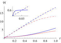
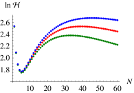
Figure 1: (a) The optimal $\mathcal{H}$ over $\theta$ as a function of time $t$ for a single measurement ($N=1$) on the damped oscillator in the non-Markovian (solid) and Markovian (dashed) baths. The thick (thin) lines are for the constant (resonant) force here and in the following plots. The inset shows the short time behavior of $\mathcal{H}$. Here $r=5$. (b) The behavior of $\mathcal{H}$ as a function of $N$ for detecting a constant force in the non-Markovian bath with $r=2.50$, $2.66$, and $2.80$ from the bottom up. Here the optimization of $\mathcal{H}$ over $\theta_{k}$ is made.

The plots of the optimal $\mathcal{H}$ over $\theta$ as a function of the measurement time $t$ are shown in Fig. 1 (a). We see that the results for the non-Markovian and Markovian baths show quite different behaviors as functions of $t$, especially at short times. As $t\to 0$, we notice that $\mathcal{H}\to{2\xi t^{2}}$ for the non-Markovian bath, and $\mathcal{H}\to{t/\gamma}$ for the Markovian bath. On the other hand, as $t\to\infty$, both of them approach to the steady value $\mathcal{H}\to b_{x}^{2}/\sigma^{\infty}_{xx}+b_{p}^{2}/\sigma^{\infty}_{pp}$. It suggests to us that for a total probing time $t_{\rm tot}$, the force sensitivity can be further improved by $N$-repeated measurements, where each part with the mean energy $E$ is probed for a time interval $\tau=t_{\rm tot}/N$. For this sequential strategy, the corresponding QFI is the sum of the QFI for each measurement step,

$$\mathcal{H} = \sum_{k=0}^{N-1}\mathbf{b}^{T}(k\tau;\tau)\mathbf{\sigma}^{-1}(\theta_{k},\tau)\mathbf{b}(k\tau;\tau),$$ (15)

which should be optimized over the variables $\theta_{k}$, $N$.

Fig. 1 (b) displays the behavior of $\mathcal{H}$ versus $N$ for detecting a constant force acting on the oscillator in the non-Markovian bath with $r=2.50$, $2.66$, and $2.80$ from the bottom up. It shows that the number $N$ that maximizes $\mathcal{H}$ depends on the value of $r$. We denote this optimal number by $N_{\rm opt}$, and $\tau_{\rm opt}=t_{\rm tot}/N_{\rm opt}$. For $r\approx 2.66$, there are two global maxima, corresponding to the values $1$ and $39$ of $N$.

Fig. 2 (a) displays the behavior of $N_{\rm opt}$ versus $r$ for the non-Markovian and Markovian baths, respectively. Fig. 2 (b) displays the behavior of $\mathcal{H}_{\rm opt}$ versus $r$. As shown in Fig. 2, we notice that for the ideal oscillator, the sequential strategy makes no improvement, and $\mathcal{H}_{\rm opt}$ is linearly proportional to $E$ bk . For the damped oscillator, a single measurement should be used for low $E$, and the sequential measurements are preferred for increasingly high $E$. It can be seen that the free oscillator presents the best force sensitivity among others. The non-Markovian result is worse than the Markovian one for low $E$, and becomes better as $E$ increases.

From Fig. 2 and for a sufficiently high $E\approx e^{2r}/4$, the optimal number $N_{\rm opt}$ can be well approximated by

$$N_{\rm opt}\approx\bigg{\{}\begin{matrix}d_{0}\sqrt{E}&\quad\text{for the non-Markovian bath},\\ c_{0}E^{1/3}&\quad\text{for the Markovian bath},\end{matrix}$$ (16)

and the corresponding optimal QFI can be fitted by

$$\mathcal{H}_{\rm opt}\approx\bigg{\{}\begin{matrix}d_{1}\sqrt{E},\\ {c_{1}/\gamma}-c_{2}E^{-{2/3}}.\end{matrix}$$ (17)

In terms of the total energy $E_{\rm tot}=NE\to\infty$ and for an arbitrary $t_{\rm tot}\gg 1$, we have

$$\mathcal{H}_{\rm opt}/t_{\rm tot}\approx\bigg{\{}\begin{matrix}d_{1}^{\prime}(E_{\rm tot}/t_{\rm tot})^{1/3}\to\infty,\\ {c^{\prime}_{1}/\gamma}-c^{\prime}_{2}(E_{\rm tot}/t_{\rm tot})^{-1/2}\to{c^{\prime}_{1}/\gamma},\end{matrix}$$ (18)

where $d_{1}^{\prime}=d_{1}(d_{0}\pi^{2}/4)^{-{1/3}}$, $c_{1}^{\prime}=2c_{1}/\pi$ and $c_{2}^{\prime}=c_{2}\sqrt{8c_{0}/\pi^{3}}$. We find that the above coefficients take: $d_{0}=5.60$ independent of the force shapes, $d_{1}=1.76$ for constant force, and $d_{1}=0.88$ for resonant force; $c_{0}=0.64$, $c_{1}=31.41$, and $c_{2}=47.81$ for constant force, $c_{0}=0.80$, $c_{1}=15.71$, and $c_{2}=30.11$ for resonant force. The Markovian results are in agreement with Eqs. (33) and (35) in Ref. latu .

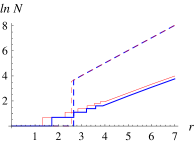
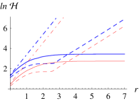
Figure 2: (a) The plots of $N_{\rm opt}$ versus the squeeze parameter $r$ for the non-Markovian (dashed) and Markovian (solid) oscillators. (b) The behavior of $\mathcal{H}_{\rm opt}$ versus $r$ for the free (dot-dashed), non-Markovian (dashed), and Markovian (solid) oscillators.

The key point demonstrated by the above numerics is that the force sensitivity with the damped oscillator initially prepared in a squeezed state performs better for the non-Markovian case when the total mean energy gets higher. Under such a situation, a relatively larger $N_{\rm opt}$ is used and hence the oscillator can benefit more from non-Markovian noise feature. Furthermore, the cube root asymptotic for $\mathcal{H}_{\rm opt}$ is not specific to our chosen model, but rather a general consequence of the unitary evolution of the total oscillator-bath state.

To put it more explicitly and following Ref. latu , we consider the limit of a fast sequential measurement, that is, $\tau$ is much smaller than all characteristic times of the process, and are able to derive an analytical expression for $N_{\rm opt}$ and $\mathcal{H}_{\rm opt}$. Using the series expansions of $G(t)=t+G_{3}t^{3}/3!+O(t^{5})$ and $\nu(t)=\nu_{0}+\nu_{2}t^{2}/2!+O(t^{4})$, the optimal angle is determined by $\theta_{k}=t/2+O(t^{2})$ from the vanishing derivative of Eq. (15) with respect to $\theta_{k}$, and therefore Eq. (15) takes the form

$$\mathcal{H}={2\tau+O(\tau^{3})\over 1/\xi+2\nu_{0}\tau^{2}+O(\tau^{4})}\int_{0}^{t_{\rm tot}}dt\varsigma^{2}(t),$$ (19)

where the Euler-Maclaurin formula has been applied to transform the summation over $k$ into an integral, and therein the boundary terms have been chosen as zero. Here the dominate term in the denominator starts from $O(t^{2})$, whereas for the Markovian case, it starts from $O(t)$ as shown in Ref. latu .

From the above equation, the optimal interval that maximizes $\mathcal{H}$ is found to be $\tau_{\rm opt}=(2\nu_{0}\xi)^{-{1/2}}+O(\xi^{-1})$, or

$$N_{\rm opt}=t_{\rm tot}\sqrt{2\nu_{0}\xi}+O(1).$$ (20)

The optimal QFI is thus

$$\mathcal{H}_{\rm opt}=\sqrt{\xi\over 2\nu_{0}}\int_{0}^{t_{\rm tot}}dt\varsigma^{2}(t)+O(1).$$ (21)

The regime of validity of Eqs. (20) and (21) are confined by the conditions $\tau_{\rm opt}\ll\mathrm{max}\{1/\gamma,1/\omega_{0},1/\Lambda,\tau_{\rm ch}\}$, where $\tau_{\rm ch}$ is the characteristic time of evolution of $\varsigma(t)$. As $E\simeq\xi/4\to\infty$, Eq. (20) implies that $N_{\rm opt}$ is independent of the force shape $\varsigma(t)$, while in Eq. (21) $\mathcal{H}_{\rm opt}$ depends on $\varsigma(t)$ through the integral $\int_{0}^{t_{\rm tot}}dt\varsigma^{2}(t)$, as confirmed by the numerical results. For the regularized Ohmic bath at zero temperature, we have $\nu_{0}=\gamma\Lambda^{2}/(2\pi)\approx 1.59$, $\int_{0}^{t_{\rm tot}}dt\varsigma^{2}(t)=t_{\rm tot}$ and $t_{\rm tot}/2$ for the constant and resonant forces, respectively. They fit the obtained numerical values quite well after crossing the point $r\approx 2.66$.

VI Conclusion

In summary, we have found that the memory effects of the surrounding bath could significantly change the short time behavior of the system evolution. Using the quantum Fisher information, we have got an exact expression for the optimal quantum limit of the force sensitivity probed by the damped oscillator prepared in the factorized initial squeezed state. The optimal force sensitivity thus obtained approaches to zero for the non-Markovian bath, whereas approaches to a finite non-zero value for the Markovian bath when the mean energy of the oscillator goes to infinity.

- (1) C.A. Regal,J.D. Teufel, and K.W. Lehnert, Nat. Phys. 4, 555 (2008); R. Maiwald, D. Leibfried, J. Britton, J.C. Bergquist, G. Leuchs, and D.J. Wineland, Nat. Phys. 5, 551 (2009); J.D. Teufel, T. Donner, M.A. Castellanos-Beltran, J.W. Harlow, and K.W. Lehnert, Nat. Nanotechnol. 4,820 (2009); M.J. Biercuk, H. Uys, J.W. Britton, A.P. VanDevender, and J.J. Bollinger, Nat. Nanotechnol. 5,646 (2010); The LIGO Scientific Collaboration, Nat. Phys. 7, 962 (2011).
- (2) M. Kacprowicz, R. Demkowicz-Dobrzanski, W. Wasilewski, K. Banaszek, and I. A. Walmsley, Nature Photonics 4, 357 (2010).
- (3) V. Giovannetti, S. Lloyd, and L. Maccone, Science 306, 1330 (2004); Phys. Rev. Lett. 96, 010401 (2006); Nat. Photonics 5, 222 (2011).
- (4) H.P. Breuer and F. Petruccione, Open Quantum Systems (Oxford University Press, Oxford, 2002).
- (5) A. Monras and M.G.A. Paris, Phys. Rev. Lett. 98, 160401 (2007); M. Aspachs, G. Adesso, and I. Fuentes, Phys. Rev. Lett. 105, 151301 (2010).
- (6) A.W. Chin, S.F. Huelga, and M.B. Plenio, Phys. Rev. Lett. 109, 233601 (2012).
- (7) M. Tsang, H.M. Wiseman, and C.M. Caves, Phys. Rev. Lett. 106, 090401 (2011).
- (8) V.B. Braginsky, Y.I. Vorontsov, and K.S. Thorne, Science 209, 547 (1980); V.B. Braginsky and F.Y. Khalili, Quantum Measurement (Cambridge University Press, UK, 1992).
- (9) C.M. Caves, K.S. Thorne, R.W.P. Drever, V.D. Sandberg, and M. Zimmerman, Rev. Mod. Phys. 52, 341 (1980).
- (10) C.W. Helstrom, Quantum Detection and Estimation Theory (Academic Press, New York, 1976); A.S. Holevo, Probabilistic and Statistical Aspects of Quantum Theory (North-Holland, Amsterdan, 1982).
- (11) S.L. Braunstein and C.M. Caves, Phys. Rev. Lett. 72, 3439 (1994).
- (12) C.L. Latune, B.M. Escher, R.L. de Matos Filho, and L. Davidovich, Phys. Rev. A 88, 042112 (2013).
- (13) B.M. Escher, R.L. de Matos Filho, and L. Davidovich, Nat. Phys. 7, 406 (2011).
- (14) F. Haake and R. Reibold, Phys. Rev. A. 32, 2462 (1985); B.L. Hu, J.P. Paz, and Y. Zhang, Phys. Rev. D. 45, 2843 (1992); R. Karrlein and H. Grabert, Phys. Rev. E. 55, 153 (1997); G.W. Ford and R.F. O’Connell, Phys. Rev. D. 64, 105020 (2001); C.H. Fleming, A. Roura, and B.L. Hu, Ann. Phys. 326, 1207 (2011).
- (15) D.F. Walls and G.J. Milburn, Quantum Optics (Springer, Berlin, 1994).
- (16) V. Hakim and V. Ambegaokar, Phys. Rev. A 32, 423 (1985).
- (17) E. Pollak, J. Shao, and D.H. Zhang, Phys. Rev. E. 77, 021107 (2008).
- (18) H. Scutaru, J. Phys. A 31, 3659 (1998).
- (19) W.J. Munro, K. Nemoto, G.J. Milburn, and S.L. Braunstein, Phys. Rev. A 66, 023819 (2002).