Random unfriendly seating arrangement
in a dining table

Abstract

A detailed study is made of the number of occupied seats in an unfriendly seating scheme with two rows of seats. An unusual identity is derived for the probability generating function, which is itself an asymptotic expansion. The identity implies particularly a local limit theorem with optimal convergence rate. Our approach relies on the resolution of Riccati equations. We also clarify some simple yet delicate stochastic dominance relations.

1 Introduction

Freedman and Shepp formulated the “unfriendly seating arrangement problem” in 1962 [15, Problem 62–3]:

There are $n$ seats in a row at a luncheonette and people sit down one at a time at random. They are unfriendly and so never sit next to one another (no moving over). What is the expected number of persons to sit down?

Let $Z_{n}$ denote the number of persons sitting down when no further customers can sit properly without breaking the restriction of unfriendliness. Solutions with different degree of precision or generality were later proposed by many. In particular, Friedman and Rothman [16] proved that

$$\mathbb{E}(Z_{n}) =\sum_{0\leqslant k<n}(n-k)\frac{(-2)^{k}}{(k+1)!}$$

$$=\tfrac{1}{2}\left(1-e^{-2}\right)(n+3)-1+O\left(\frac{2^{n}}{(n+2)!}\right),$$

for large $n$. The factorial error term here seems characteristic of sequential models of a similar nature; see, for example, (1), (22) and (24) below and [6]. We will provide a general framework for characterizing such small errors; see Proposition 1 below. In addition, Friedman and Rothman　[16] extended the “degree of unfriendliness” to any　integer $b\geqslant 1$, where any two people have to sit with at least $b$ unoccupied seats between them. This extension was mentioned to be related to Rényi’s Parking Problem and to a discrete parking problem studied by MacKenzie (see [21]) in which cars of the same length $\ell\geqslant 2$ are parked uniformly at random along the curb with $n$ unit parking spaces. Indeed, the latter problem with $\ell=2$ found its origin in Flory’s 1939 pioneering paper [14] in polymer chemistry, and was later expanded into generic stochastic models under the name “random sequential adsorption”; see [7] for a comprehensive survey and [2, 8, 24, 25] a more recent account.

Due to the simplicity and the usefulness of the model, the same discrete parking problem was also studied independently under different guises in applied probability and related areas. Page [22] studied a random pairing model in which $n$ isolated points are paired randomly by adjacency until only singletons remain. This model is identical to Flory’s monomer-dimer model [14] (or the discrete parking problem [21] where each car requires 2-unit parking space). The same model was also encountered in a few diverse modeling contexts. Let $\zeta_{n}$ denote the resulting number of pairs when no more adjacent pair can be formed. Then it is easy to see that

$$Z_{n}\equiv\tfrac{1}{2}\zeta_{n+1}\qquad(n\geqslant 0).$$

In addition to deriving a closed-form expression for the first three moments of $\zeta_{n}$, Page [22] also computed the variance, which, when transferring to our $Z_{n}$, satisfies

$$\mathbb{V}(Z_{n})=\binom{n+1}{2}-\mu_{n}^{2}-\sum_{0\leqslant k\leqslant n-2}\frac{(-2)^{k}}{(k+2)!}\binom{n-k}{2}\left(2^{k}(k-2)+k^{2}+4k+6\right);$$

asymptotically,

$$\mathbb{V}(Z_{n})=e^{-4}(n+3)+O\left(\frac{4^{n}}{(n+2)!}\right).$$ (1)

Another interesting result in [22] is the closed-form expression for the bivariate generating function of $\mathbb{E}(t^{\zeta_{n}})$, obtained by solving a Riccati equation; see also [27]. In terms of $Z_{n}$, this closed-form translates into

$$\sum_{n\geqslant 0}\mathbb{E}\left(t^{Z_{n}}\right)z^{n}=\frac{\sqrt{t}\left(\left(1+\sqrt{t}\right)e^{2\sqrt{t}z}+1-\sqrt{t}\right)}{\left(1+\sqrt{t}\right)\left(1-\sqrt{t}z\right)e^{2\sqrt{t}z}-\left(1-\sqrt{t}\right)\left(1+\sqrt{t}z\right)}.$$ (2)

Page predicted that the $\zeta_{n}$’s were asymptotically normally distributed, which was later proved by Runnenburg [27] by the method of moments; see [20] for an extension. See also [4, 5, 11] for other properties studied. The asymptotic normality is contained as a special case of Penrose and Sudbury’s very general central limit theorem in [26], where they also derived a convergence rate by Stein’s method.

The exact solvability of such a model is however very rare in the literature, and the next possibly solvable cases are the unfriendly variants for two rows of seats with the same rule of nearest neighbors exclusion, which we may refer to as the unfriendly seating arrangement in a dining table. Such a model and the like were studied by physicists in the 1990’s and the “jamming density” (the large-$n$ limit of the ratio between the expected number of persons sitting down and the total number of seats) was given explicitly by

$$\tfrac{1}{4}\left(2-e^{-1}\right)\approx 0.408030\dots$$ (3)

using different heuristic arguments; see [1, 9]. This constant is to be compared with that in the one-row case

$$\tfrac{1}{2}\left(1-e^{-2}\right)\approx 0.432332\dots;$$

see also Finch’s book [10, §5.3.1] for more information.

The same problem was recently reformulated as the unfriendly theater seating arrangement problem by Georgiou et al. [17], where they indeed addressed the configuration of $m$ rows of seats (mentioned to be connected to maximal independent sets of planar lattice) and proved the existence of the expected proportion of occupied seats. In particular, they also derived the jamming limit (3). Unfortunately, the crucial stochastic dominance relations used in their paper [17] are incorrect, and thus their proofs remain incomplete (the asymptotic linearity being well expected though). More precisely, they claimed that if $H$ is an induced subgraph of $G$, then the first-order stochastic dominance relation $X_{H}\leqslant X_{G}$ holds in the sense that

$$\mathbb{P}\left(X_{H}>k\right)\leqslant\mathbb{P}\left(X_{G}>k\right),$$ (4)

for all $k$, where $X_{H},X_{G}$ are the random variables counting the number of occupied seats (or the cardinality of an independent set) when starting with the seat configurations $H$ and $G$, respectively, and following the same random unfriendly seating procedure until the procedure terminates. It is known that this implies the second-order stochastic dominance

$$\mathbb{E}(X_{H})\leqslant\mathbb{E}(X_{G}).$$ (5)

Unfortunately, none of the two relations (4) and (5) is correct. Here is a counterexample to (4). If the two initial seat configurations are given as follows

$$H_{1}=\begin{array}[]{lll}&\bigcirc&\\ \bigcirc&\bigcirc&\bigcirc\end{array}\quad\text{and}\quad G_{1}=\begin{array}[]{lll}\bigcirc&\bigcirc&\\ \bigcirc&\bigcirc&\bigcirc\end{array},$$

then

$$\begin{cases}\mathbb{P}(X_{H_{1}}=1)=\frac{1}{4}\\ \mathbb{P}(X_{H_{1}}=3)=\frac{3}{4},\end{cases}\quad\text{and}\quad\begin{cases}\mathbb{P}(X_{G_{1}}=2)=\frac{7}{15}\\ \mathbb{P}(X_{G_{1}}=3)=\frac{8}{15}.\end{cases}$$

implying that

$$\mathbb{P}(X_{H_{1}}\geqslant 3)>\mathbb{P}(X_{G_{1}}\geqslant 3),$$

contrary to (4). For a counterexample to (5), consider the following two seat configurations

$$H_{2}=\begin{array}[]{ll}\bigcirc&\\ &\bigcirc\end{array},\quad G_{2}=\begin{array}[]{ll}\bigcirc&\\ \bigcirc&\bigcirc\end{array}.$$

Then the expected numbers of occupied seats satisfy $\mathbb{E}[X_{H_{2}}]=2>\mathbb{E}[X_{G_{2}}]=5/3$.

Due to the subtlety of the problem, we focus our attention in this paper on the dining table model and we show that this model is also explicitly solvable by solving a system of nonlinear differential equations. This new result leads to interesting structural properties, and many strong limit theorems will then follow. In particular, our analysis provides the first rigorous, complete proof for the very simple jamming limit (3) with an optimal error terms. Some related stochastic dominance relations will be clarified in Section 6.

2 Recurrences and solutions

We consider a dining table with $2n$ seats arranged in two rows

$$\mathscr{X}_{n}:=\begin{array}[]{l}\overbrace{\begin{array}[]{lllllllll}\bigcirc&\bigcirc&\bigcirc&\bigcirc&\bigcirc&\cdots&\bigcirc&\bigcirc&\bigcirc\end{array}}^{n}\\ \begin{array}[]{lllllllll}\bigcirc&\bigcirc&\bigcirc&\bigcirc&\bigcirc&\cdots&\bigcirc&\bigcirc&\bigcirc\end{array}\end{array}$$ (10)

Diners arrive one after another and each selects a seat uniformly at random. If the seat is empty, then it becomes occupied, and two of its neighboring seats together with the opposite one (in the other row) are no more available. If the seat selected is occupied or forbidden and there are still empty seats available, then the (uniform) random selection is repeated until a seat is found. The process stops as long as all seats are either occupied or forbidden. An example with $n=10$ is given as follows (where “ $\oslash$ ” stands for a forbidden seat and “ $\bullet$ ” an occupied seat)

$$\begin{array}[]{llllllllll}\raisebox{-0.86108pt}{\scalebox{1.5}{$\oslash$}}&\raisebox{-3.7889pt}{\scalebox{2.7}{$\bullet$}}&\raisebox{-0.86108pt}{\scalebox{1.5}{$\oslash$}}&\raisebox{-0.86108pt}{\scalebox{1.5}{$\oslash$}}&\raisebox{-0.86108pt}{\scalebox{1.5}{$\oslash$}}&\raisebox{-3.7889pt}{\scalebox{2.7}{$\bullet$}}&\raisebox{-0.86108pt}{\scalebox{1.5}{$\oslash$}}&\raisebox{-0.86108pt}{\scalebox{1.5}{$\oslash$}}&\raisebox{-3.7889pt}{\scalebox{2.7}{$\bullet$}}&\raisebox{-0.86108pt}{\scalebox{1.5}{$\oslash$}}\\ \raisebox{-3.7889pt}{\scalebox{2.7}{$\bullet$}}&\raisebox{-0.86108pt}{\scalebox{1.5}{$\oslash$}}&\raisebox{-0.86108pt}{\scalebox{1.5}{$\oslash$}}&\raisebox{-3.7889pt}{\scalebox{2.7}{$\bullet$}}&\raisebox{-0.86108pt}{\scalebox{1.5}{$\oslash$}}&\raisebox{-0.86108pt}{\scalebox{1.5}{$\oslash$}}&\raisebox{-3.7889pt}{\scalebox{2.7}{$\bullet$}}&\raisebox{-0.86108pt}{\scalebox{1.5}{$\oslash$}}&\raisebox{-0.86108pt}{\scalebox{1.5}{$\oslash$}}&\raisebox{-3.7889pt}{\scalebox{2.7}{$\bullet$}}\end{array}.$$

Let $X_{n}$ count the total number of persons sitting down when such a sequential process terminates. Then it is easy to see that

$$\left\lfloor n/2\right\rfloor+1\leqslant X_{n}\leqslant n\qquad(n\geqslant 1).$$

By splitting the $2n$-problem at the first occupied seat into two subproblems, we are then led to the recurrence relation for the probability generating function $X_{n}(t):=\mathbb{E}(t^{X_{n}})$

$$X_{n}(t)=\frac{t}{n}\sum_{0\leqslant k\leqslant n-1}Y_{k}(t)Y_{n-1-k}(t)\qquad(n\geqslant 1),$$ (11)

with $X_{0}(t)=1$. Here $Y_{n}$ counts the number of occupied seats under the same unfriendly seating procedure but with the slightly different initial configuration of the seats

$$\mathscr{Y}_{n}:=\begin{array}[]{l}\overbrace{\begin{array}[]{llllllll}\bigcirc&\bigcirc&\bigcirc&\bigcirc&\bigcirc&\cdots&\bigcirc&\bigcirc\end{array}}^{n-1}\\ \begin{array}[]{lllllllll}\bigcirc&\bigcirc&\bigcirc&\bigcirc&\bigcirc&\cdots&\bigcirc&\bigcirc&\bigcirc\end{array}\end{array}$$ (16)

where the total number of seats is $2n-1$. The following two diagrams show the obvious decompositions after the first seat is occupied.

Applying the same conditioning argument to $Y_{n}$, we need to introduce two additional sequences of random variables based on the following seat configurations: for $n\geqslant 1$

$$\mathscr{A}_{-1} =\mathscr{A}_{0}=\varnothing,$$

$$\mathscr{A}_{n} :=\begin{array}[]{l}\overbrace{\begin{array}[]{lllllllll}\bigcirc&\bigcirc&\bigcirc&\bigcirc&\bigcirc&\cdots&\bigcirc&\bigcirc&\bigcirc\end{array}}^{n}\\ \hskip 23.33147pt\begin{array}[]{lllllllll}\bigcirc&\bigcirc&\bigcirc&\bigcirc&\bigcirc&\cdots&\bigcirc&\bigcirc&\bigcirc\end{array}\end{array}$$

and

$$\mathscr{B}_{-1} =\varnothing,\;\mathscr{B}_{0}=\bigcirc,$$

$$\mathscr{B}_{n} :=\begin{array}[]{c}\hskip 23.33147pt\overbrace{\begin{array}[]{llllllll}\bigcirc&\bigcirc&\bigcirc&\bigcirc&\cdots&\bigcirc&\bigcirc&\bigcirc\end{array}}^{n-1}\\ \hskip 23.33147pt\begin{array}[]{llllllllll}\bigcirc&\bigcirc&\bigcirc&\bigcirc&\bigcirc&\cdots&\bigcirc&\bigcirc&\bigcirc&\bigcirc\end{array}\end{array}$$

Let $A_{n}$, and $B_{n}$ denote the number of sitting persons under the same unfriendly seating procedure when started from the configurations $\mathscr{A}_{n}$ and $\mathscr{B}_{n}$, respectively. The initial conditions are defined to be $A_{-1}=A_{0}=0$ and $B_{-1}=0,B_{0}=1$. Then we have the following systems of recurrences.

Lemma 1.

The probability generating functions $A_{n}(t),B_{n}(t)$ and $Y_{n}(t)$ satisfy

$$\begin{cases}\displaystyle A_{n}(t)=\frac{t}{n}\sum_{1\leqslant k\leqslant n}A_{k-2}(t)B_{n-k}(t),\\ \displaystyle B_{n}(t)=\frac{t}{2n}\left(\sum_{1\leqslant k\leqslant n-1}B_{k-1}(t)B_{n-1-k}(t)+\sum_{1\leqslant k\leqslant n+1}A_{k-2}(t)A_{n-k}(t)\right),\end{cases}$$ (17)

and

$$Y_{n}(t)=\frac{t}{2n-1}\left(\sum_{0\leqslant k\leqslant n-2}Y_{k}(t)B_{n-2-k}(t)+\sum_{0\leqslant k\leqslant n-1}Y_{k}(t)A_{n-2-k}(t)\right),$$

for $n\geqslant 1$ with the initial conditions $A_{n}(t)=B_{n}(t)=Y_{n}(t)=1$ if $n<0$ and $A_{0}(t)=Y_{0}(t)=1$ and $B_{0}(t)=t$.

Proof.

After the first diner sits down, the random variable $Y_{n}$ is decomposed in either the following two ways.

Similarly, the random variable $A_{n}$ is decomposed as follows

And, finally, we have the two possible decompositions for $B_{n}$

The lemma follows by computing the corresponding probabilities. ∎

Consider now $G_{A}(z,t):=\sum_{n\geqslant 0}\mathbb{E}\left(t^{A_{n}}\right)z^{n}$, the bivariate generating function of $A_{n}$. The notations $G_{B}(z,t)$ and $G_{Y}(z,t)$ are defined similarly. Then Lemma 1 implies the following system of Riccati equations.

Lemma 2.

The bivariate generating functions $G_{A},G_{B}$ satisfy

$$\begin{cases}G_{A}^{\prime}=tG_{B}+tzG_{A}G_{B},\\ \displaystyle G_{B}^{\prime}=tG_{A}+\frac{tz}{2}\left(G_{A}^{2}+G_{B}^{2}\right),\end{cases}$$

with $G_{A}(0,t)=1$ and $G_{B}(0,t)=t$, and

$$2zG_{Y}^{\prime}=\left(1+tz+tz^{2}(G_{A}+G_{B})\right)G_{Y}-1,$$

with $G_{Y}(0,t)=1$. Here for simplicity $G_{\bullet}=G_{\bullet}(z,t)$ and $G_{\bullet}^{\prime}:=(\partial/\partial z)G_{\bullet}(z,t)$.

These equations admit explicit solutions as follows. Define

$$U(z,t)=\frac{2t(1+t)}{(1+t)(1-tz)-(1-t)e^{-tz}}.$$ (18)

Lemma 3.

We have

$$G_{A}(z,t)=\frac{U(z,t)+U(z,-t)}{2},\quad G_{B}(z,t)=\frac{U(z,t)-U(z,-t)}{2},$$ (19)

and

$$G_{Y}(z,t)=\frac{Q(z,t)}{P(z,t)},$$ (20)

where

$$P(z,t) =(1+t)(1-tz)-(1-t)e^{-tz},$$

$$Q(z,t) =1+t-(1-t)e^{-tz}-\frac{1-t}{2}\,tz\int_{0}^{1}e^{-tz(1+v)/2}v^{-1/2}{\,\rm d}v.$$

Note that $Q$ can be expressed in terms of the error function or the standard normal distribution function $\Phi$. For example,

$$Q(z,t)=1+t-(1-t)e^{-tz/2}\left(e^{-tz/2}-\sqrt{\frac{\pi}{2}tz}+\sqrt{2\pi tz}\,\Phi(\sqrt{tz})\right).$$

Proof.

For convenience, define $V(z,t):=U(z,-t)$. Then $U=G_{A}+G_{B}$ and $V=G_{A}-G_{B}$ satisfy the simpler equations

$$\begin{cases}\displaystyle U^{\prime}=tU+\frac{tz}{2}U^{2},\\ \displaystyle V^{\prime}=-tV-\frac{tz}{2}V^{2},\end{cases}$$

with $U(0,t)=1+t$ and $V(0,t)=1-t$. Since this is a system of Bernoulli equations, we consider the transformation $u=-U^{-1}$, which satisfies the equation

$$u^{\prime}+tu=\frac{tz}{2},$$

with $u(0,t)=-1/(1+t)$. Solving this equation gives (18), and (19) follows.

For $G_{Y}$, we then have the first-order differential equation

$$2zG_{Y}^{\prime}=\left(1+tz+tz^{2}U\right)G_{Y}-1.$$

To solve this equation, we consider $\tilde{G}_{Y}:=G_{Y}-1$ and introduce the integration factor

$$I(z)=I(z,t):=z^{-1/2}e^{tz/2}P(z,t).$$

Then

$$(I\cdot\tilde{G}_{Y})^{\prime}=\frac{tI}{2}(1+zU),$$

with $\tilde{G}_{Y}(0,t)=0$, which has the solution

$$\tilde{G}_{Y}(z,t)=\frac{t}{2I(z)}\int_{0}^{z}I(s)(1+sU(s,t)){\,\rm d}s.$$

Note that

$$I(z,t)(1+zU(z,t))=z^{-1/2}\left((1+t)(1+zt)e^{tz/2}-(1-t)e^{-tz/2}\right).$$

Then

$$\int_{0}^{z}I(s,t)\left(1+sU(s,t)\right){\,\rm d}s$$

$$\qquad=2\sqrt{z}(1+t)e^{tz/2}-(1-t)\int_{0}^{z}s^{-1/2}e^{-ts/2}{\,\rm d}s$$

$$\qquad=2\sqrt{z}(1+t){\rm e}^{tz/2}-(1-t)\sqrt{z}\int_{0}^{1}v^{-1/2}e^{-tzv/2}{\,\rm d}v.$$

Thus

$$\widetilde{G}_{Y}(z,t) =\frac{Q(z,t)}{P(z,t)}=1+\frac{t}{2I(z,t)}\int_{0}^{z}I(s,t)\left(1+sU(s,t)\right){\,\rm d}s$$

$$=\frac{1}{P(z,t)}\left(1+t-(1-t)e^{-tz}-\frac{t(1-t)}{2}z\int_{0}^{1}e^{-tz(1+v)/2}v^{-1/2}{\,\rm d}v\right),$$

which proves (20). ∎

Returning to $X_{n}$, by (11), we have

$$G_{X}(z,t):=\sum_{n\geqslant 0}\mathbb{E}\left(t^{A_{n}}\right)z^{n}=1+t\int_{0}^{z}G_{Y}(u,t)^{2}{\,\rm d}u.$$ (21)

Since the uniform splitting procedure also arises naturally in diverse algorithmic and combinatorial contexts, Riccati equations were often encountered in related literature; see, for example, [12, 23].

3 Mean and variance

With the explicit expressions derived above, we have two different approaches to compute the mean and the variance: one based on a direct use of (21) and a suitable manipulation of the error terms (see [13, Ch. VII]) and the other depending on Quasi-Power type argument (see [13, §IX. 5],[18]). While both approaches provide readily the two dominant asymptotic terms, the characterization of the extremely small error requires a more careful analysis. For methodological interest, we discuss the first approach here by providing a general means for error analysis, which will also be useful for problems of a similar nature. The second approach will be briefly indicated later.

Theorem 1.

The mean of $X_{n}$ satisfies

$$\mathbb{E}(X_{n})=\mu n+c_{1}+O\left(\frac{1}{(n+3)!}\right),$$ (22)

where $\mu:=1-e^{-1}/2$ and ($\phi:=2\Phi(1)-1$)

$$c_{1}:=\frac{e^{-1}}{2}\left(\sqrt{2\pi e}\,\phi-1\right)\approx 0.33502\,27062\,94844\dots,$$ (23)

and the variance satisfies

$$\mathbb{V}(X_{n})=\sigma^{2}n+c_{2}+O\left(\frac{2^{n}}{(n+4)!}\right),$$ (24)

where $\sigma:=\sqrt{\frac{3}{4}}\,e^{-1}$ and

$$\begin{split}c_{2}:=\frac{e^{-2}}{4}\left(-\pi e\phi^{2}-2\sqrt{2\pi e}\,\phi+5\right)\approx-0.15640\,75038\,00915\dots{}\end{split}$$ (25)

From (22), we see that the jamming density is given by

$$\lim_{n\to\infty}\frac{\mathbb{E}(X_{n})}{2n}=\tfrac{1}{4}\left(2-e^{-1}\right).$$

Also the $O$-terms in (22) and (24) are smaller than the corresponding ones in the one-row version.

Proof.

From (20), we have

$$M_{Y}(z) :=\sum_{n\geqslant 0}\mathbb{E}(Y_{n})z^{n}=\frac{\partial}{\partial t}\,G_{Y}(z,t)\Bigr{|}_{t=1}$$

$$=\frac{z}{(1-z)^{2}}\left(1-\frac{e^{-z}}{2}\right)+\frac{z}{4(1-z)}\int_{0}^{1}v^{-1/2}e^{-(1+v)z/2}{\,\rm d}v.$$

Then we deduce that

$$M_{X}(z) :=\sum_{n\geqslant 0}\mathbb{E}(X_{n})z^{n}=2\int_{0}^{z}\frac{M_{Y}(u)}{1-u}{\,\rm d}u+\int_{0}^{z}\frac{1}{(1-u)^{2}}{\,\rm d}u$$ (26)

$$=\frac{\mu}{(1-z)^{2}}+\frac{c_{0}}{1-z}+O(1),$$

as $z\sim 1$, where

$$c_{0}:=-1+\frac{\sqrt{\pi}}{\sqrt{2e}}\left(2\Phi(1)-1\right)=-1+\frac{\sqrt{\pi}}{\sqrt{2e}}\,\phi.$$

Consequently, by standard singularity analysis [13, Ch. VII],

$$\mathbb{E}(X_{n})=\mu n+c_{1}+O\left(n^{-K}\right),$$ (27)

for any $K>0$.

The leading terms in (24) for the variance are computed similarly.

Numerically, the approximation (27) without the $O$-term is extremely good even for small values of $n$; see Figure 1. For example, the error term is already less than $10^{-7}$ when $n\geqslant 8$.

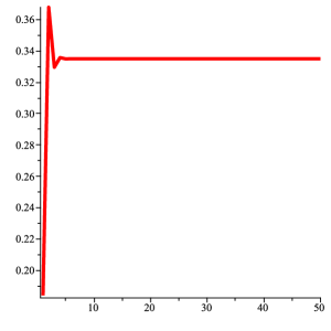
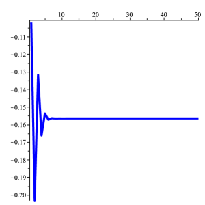
Figure 1: Goodness of the approximations (27) and (24) by computing the exact values of $\mathbb{E}(X_{n})-\mu n$ (left) and $\mathbb{V}(X_{n})-\sigma^{2}n$ (right) for $n=1,\dots,50$.

To clarify the rapid convergence of the mean and variance towards their limit (see Figure 1), we refine the asymptotic approximation (27) by the following simple error analysis. Note first that we are dealing with asymptotics of the form ($[z^{n}]f(z)$ denoting the coefficient of $z^{n}$ in the Taylor expansion of $f$)

$$[z^{n}]\frac{f(z)}{(1-z)^{m}},\quad[z^{n}]\int_{0}^{z}\frac{f(u)}{(1-u)^{m}}\,{\,\rm d}u,$$

where $m=1,2,\dots$ and $f$ is an entire function with quickly decreasing coefficients.

Proposition 1.

If $f$ is an entire function whose coefficients satisfy

$$[z^{n}]f(z)=O\left(\varepsilon_{n}\right),$$

where $\varepsilon_{n}$ is a positive sequence satisfying $\varepsilon_{n}=O(K^{-n})$ for some $K>1$, then, for $m=1,2,\dots$,

$$[z^{n}]\frac{f(z)}{(1-z)^{m}}=\sum_{0\leqslant j<m}\frac{(-1)^{j}}{j!}\,f^{(j)}(1)\binom{n+m-1-j}{m-1-j}+O(|\varepsilon_{n+m}|),$$ (28)

and

$$[z^{n}]\int_{0}^{z}\frac{f(u)}{(1-u)^{m}}\,{\,\rm d}u=\frac{1}{n}\sum_{0\leqslant j<m}\frac{(-1)^{j}}{j!}\,f^{(j)}(1)\binom{n+m-2-j}{m-1-j}+O\left(\frac{|\varepsilon_{n+m-1}|}{n}\right).$$ (29)

Proof.

Let $f_{n}:=[z^{n}]f(z)$. Then

$$[z^{n}]\frac{f(z)}{(1-z)^{m}}=\sum_{0\leqslant k\leqslant n}\binom{n+m-k-1}{m-1}f_{k}=\sum_{k\geqslant 0}\binom{n+m-k-1}{m-1}f_{k}-\delta_{n},$$

where

$$\delta_{n}:=\sum_{k\geqslant n+m}\binom{n+m-k-1}{m-1}f_{k}=O\left(|\varepsilon_{n+m}|)\right).$$

On the other hand, by expanding $f(z)$ at $z=1$ and computing the coefficients term by term, we have the identity ($f_{k}=f^{(k)}(0)/k!$)

$$\sum_{k\geqslant 0}\frac{f^{(k)}(0)}{k!}\binom{n+m-k-1}{m-1}=\sum_{0\leqslant j<m}(-1)^{j}\frac{f^{(j)}(1)}{j!}\binom{n+m-1-j}{m-1-j}.$$

This proves (28). For (29), we have

$$[z^{n}]\int_{0}^{z}\frac{f(u)}{(1-u)^{m}}\,{\,\rm d}u=\frac{1}{n}\sum_{0\leqslant k<n}\binom{n+m-k-2}{m-1}f_{k}.$$

Then (29) follows by the same analysis by replacing $n$ by $n-1$. ∎

Our analysis indeed applies to a wider class of $f$ but we do not need this in this paper.

We now apply this lemma to $M_{X}(z)$, which has the form

$$M_{X}(z)=\int_{0}^{z}\frac{f_{1}(u)}{(1-u)^{3}}{\,\rm d}u,$$

where

$$f_{1}(z)=1+z-\frac{z^{2}}{2}\int_{0}^{1}v^{-1/2}(1-v)e^{-(1+v)z/2}{\,\rm d}v.$$

Thus for $n\geqslant 2$

$$[z^{n}]f_{1}(z)=\frac{(-1)^{n-1}}{(n-2)!}\sum_{0\leqslant j\leqslant n-2}\binom{n-2}{j}(-1)^{j}\frac{(j+1)!\sqrt{\pi}}{\Gamma(j+5/2)2^{j+1}}.$$

By the standard integral representation for finite differences (Rice’s formula), we deduce that

$$[z^{n}]f_{1}(z)=2\frac{(-1)^{n-1}}{n!}\left(1+\frac{2}{n+1}+O\left(n^{-2}\right)\right).$$ (30)

Indeed, one obtains the (divergent) full asymptotic expansion

$$[z^{n}]f_{1}(z)\sim 2\frac{(-1)^{n-1}}{n!}\left(1+\sum_{k\geqslant 3}\frac{(k-1)(2k-4)!}{2^{k-2}(k-2)!}\cdot\frac{1}{(n+1)\cdots(n+k-2)}\right).$$

On the other hand, we also have

$$f_{1}(1)=2-e^{-1},\quad\text{and}\quad f_{1}^{\prime}(1)=c_{0};$$

see (26). Applying now (29) gives not only the leading terms $\mu n+c_{1}$ for $\mathbb{E}(X_{n})$ but also the precise error term in (22).

In a similar way, we have

$$S_{Y}(z) :=\sum_{n\geqslant 0}\mathbb{E}(Y_{n}^{2})z^{n}=\frac{\partial^{2}}{\partial t^{2}}G_{Y}(z,t)\Biggr{|}_{t=1}+\frac{\partial}{\partial t}G_{Y}(z,t)\Biggr{|}_{t=1}$$

$$=\frac{z(2(1+z)-(1+z)^{2}e^{-z}+e^{-2z})}{2(1-z)^{3}}+\frac{\sqrt{2\pi z}}{4(1-z)^{2}}\,e^{-z/2}(1+z^{2}-e^{-z}).$$

It follows that

$$S_{X}(z):=\sum_{n\geqslant 0}\mathbb{E}(X_{n}^{2})z^{n}=\int_{0}^{z}\frac{f_{2}(u)}{(1-u)^{4}}\,{\,\rm d}u,$$

where

$$f_{2}(z) =\tfrac{1}{2}f_{1}(z)^{2}-e^{-z}f_{1}(z)+(z^{2}-z+2)f_{1}(z)$$

$$\qquad+(1-z)(1+2z)e^{-z}-\tfrac{1}{2}(1-z)^{2}(3+2z).$$

Consider now $[z^{n}]f_{2}(z)$. By (30), we see that the first two terms on the right-hand side dominate and contribute an order bounded above by

$$[z^{n}]\left(\tfrac{1}{2}f_{1}(z)^{2}-e^{-z}f_{1}(z)\right)\leqslant 4\sum_{2\leqslant k\leqslant n-2}\frac{1}{k!(n-k)!}=O\left(\frac{2^{n}}{n!}\right),$$

the remaining terms being of order $O(1/n!)$. Thus

$$[z^{n}]f_{2}(z)=O\left(\frac{2^{n}}{n!}\right).$$

By another application of (29), we derive an asymptotic approximation to the second moment with an error term of the form $O(2^{n}/(n+4)!)$, which, together with (22), proves (24). ∎

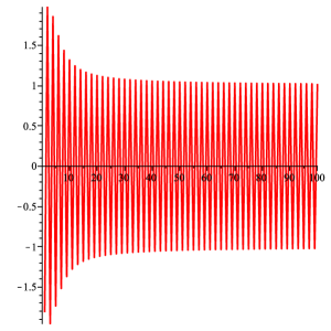
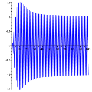
Figure 2: The factorial errors of (22) and (24): $(\mathbb{E}(X_{n})-\mu n-c_{1})(n+3)!/2$ (left) and $(\mathbb{V}(X_{n})-\sigma^{2}n-c_{2})(n+4)!/2^{n+5}$ (right) for $n=1,\dots,100$.

4 An identity for $X_{n}(t)$

Since solutions to Riccati equations have only simple poles, we expect, from the closed-form expression (20), that

$$G_{Y}(z,t)=\frac{Q(z,t)}{P(z,t)}\approx\sum_{k\in\mathbb{Z}}\frac{R_{k}(t)}{\rho_{k}(t)-z},$$ (31)

where $\rho_{k}(t)$ ranges over all zeros of $P(z,t)$ (as a function of $z$) and

$$R_{k}(t):=-\frac{Q(\rho_{k}(t),t)}{P^{\prime}(\rho_{k}(t),t)},$$

Here and throughout this section $P^{\prime}(z_{0},t)=(\partial/\partial z)P(z,t)|_{z=z_{0}}$. The expansion (31) is roughly true up to correction terms in the series to guarantee convergence; see (39). From this series, we in turn expect that

$$Y_{n}(t)=\mathbb{E}\left(t^{Y_{n}}\right)\stackrel{{\scriptstyle?}}{{=}}\sum_{k\in\mathbb{Z}}R_{k}(t)\rho_{k}(t)^{-n-1},$$

which is indeed true for $n\geqslant 1$; see (40). What is less expected is that their convolution (11), which yields $X_{n}(t)$, also admits a closed-form expression.

Before stating the identity for $X_{n}(t)$, we start with a brief discussion for the zeros of $P(z,t)$, namely,

$$(1-tz)e^{tz}=\frac{1-t}{1+t},$$

which are easily seen to be expressible in terms of Lambert’s W-functions [3]. They are the solutions to the equation

$$W(z)e^{W(z)}=z.$$ (32)

This equation has an infinity number of solutions $W_{k}(z)$, $k\in\mathbb{Z}$, and among them only one, denoted by $W(z)=W_{0}(z)$, is analytic at the origin. This function has the Taylor series expansion

$$W(z)=-\sum_{k\geqslant 1}\frac{k^{k-1}}{k!}\,(-z)^{k},$$ (33)

and has the branch cut $(-\infty,-e^{-1})$. All other solutions have the branch cut $(-\infty,0]$.

With these solutions, we have $P(\rho_{k}(t),t)=0$ when

$$\rho_{k}(t)=\frac{1}{t}\left(1+W_{k}\left(-e^{-1}\frac{1-t}{1+t}\right)\right),$$

where $\rho_{0}(t)$ has the branch cut $[-1,0]$ and the other branches the cut $[-1,1]$. As $t\to 1$, all solutions blow up to infinity except for $\rho_{0}$ which equals $1$ at $t=1$.

A useful expansion that will be needed is the following convergent series (see [3])

$$W_{k}(z)=\log z+2k\pi\mathbf{i}-\log(\log z+2k\pi\mathbf{i})+\sum_{j\geqslant 0}\frac{\Pi_{j}(\log(\log z+2k\pi\mathbf{i}))}{(\log z+2k\pi\mathbf{i})^{j}},$$

valid for all $z$, where $\Pi_{j}(x)$ is a polynomial in $x$ of degree $j$. In particular, this gives for finite $z$ and $n\neq 0$

$$|W_{k}(z)|=O(k+|\log z|).$$ (34)

Theorem 2.

For $n\geqslant 1$, we have the identity

$$X_{n}(t)=t\sum_{k\in\mathbb{Z}}R_{k}(t)^{2}\rho_{k}(t)^{-n-1},$$ (35)

for $n\geqslant 1$ and $t\in\mathbb{C}\setminus\{-1\}$, where

$$R_{k}(t):=\frac{1}{t}\left(1-\frac{1-t}{2(1+t)}\int_{0}^{1}v^{-1/2}e^{-t\rho_{k}(t)(1+v)/2}{\,\rm d}v\right).$$

When $t=-1$, we have the identity

$$X_{n}(-1)=-\frac{(-2)^{n-1}}{n}\sum_{0\leqslant k<n}\frac{k!(n-1-k)!}{(2k)!(2n-2-2k)!},$$ (36)

and the asymptotic approximation

$$X_{n}(-1)=2\frac{n!(-4)^{n}}{(2n)!\sqrt{\pi n}}\left(1+\frac{9}{8n}+O\left(n^{-2}\right)\right).$$ (37)

The expression (35) is not only an identity but also an asymptotic expansion for large $n$ (finite $t$). The left-hand side is by definition a polynomial of degree $n$, while the right-hand side is an infinite series of exponentially decreasing terms. It implies particularly that $X_{n}(t)$ is roughly of the exponential order $|\rho_{0}(t)^{-n}|$ except when $t=-1$ at which $X_{n}(t)$ is factorially small. Although $R_{k}$ can be further expressed in terms of known functions, the expression we give here is more transparent and valid for all $t\in\mathbb{C}\setminus\{-1\}$.

Proof.

We start from the local expansion

$$G_{Y}(z,t)\sim\frac{R(\rho(t),t)}{\rho(t)-z},$$

as $z\sim\rho(t)$, where $P(\rho(t),t)=0$ and

$$R(z,t):=-\frac{Q(z,t)}{P^{\prime}(z,t)}=\frac{1}{t}\left(1-\frac{1-t}{2(1+t)}\int_{0}^{1}v^{-1/2}e^{-tz(1+v)/2}{\,\rm d}v\right).$$

A more precise expansion is given as follows

$$G_{Y}(z,t) =\frac{R(\rho(t),t)}{\rho(t)-z}+\frac{Q^{\prime}(\rho(t),t)}{P^{\prime}(\rho(t),t)}-\frac{Q(\rho(t),t)P^{\prime\prime}(\rho(t),t)}{2P^{\prime}(\rho(t),t)^{2}}+O(|z-\rho(t)|)$$

$$=\frac{R(\rho(t),t)}{\rho(t)-z}+O(|z-\rho(t)|),$$

where the constant term turns out to be identically zero because

$$\begin{split}&2P^{\prime}(z,t)Q^{\prime}(z,t)-Q(z,t)P^{\prime\prime}(z,t)=\frac{t^{2}(1-t)}{2}\,P(z,t)\int_{0}^{1}v^{-1/2}e^{-tz(1+v)/2}{\,\rm d}v.\end{split}$$ (38)

This is crucial in proving (35).

Since all zeros of the $P(z,t)$ are simple, we have the partial fraction expansion

$$G_{Y}(z,t)=1+\sum_{j\in\mathbb{Z}}R_{j}(t)\left(\frac{1}{\rho_{j}(t)-z}-\frac{1}{\rho_{j}(t)}\right),$$ (39)

by the classical procedure for meromorphic functions (see [28, §3.2]), where we used the estimate (34) for $W_{k}$ (see [3]) and the asymptotic approximation

$$2\Phi(\sqrt{x})-1\sim 1-\sqrt{\frac{2}{\pi}}\,x^{-1/2}e^{-x/2}\qquad(x\to\infty).$$

This implies the identity

$$Y_{n}(t)=\sum_{j\in\mathbb{Z}}R_{j}(t)\rho_{j}(t)^{-n-1}\qquad(n\geqslant 1).$$ (40)

To prove (35), we start with the convolution (11)

$$X_{n}(t) =\frac{2t}{n}\,Y_{n-1}(t)+\frac{t}{n}\sum_{1\leqslant k\leqslant n-2}Y_{k}(t)Y_{n-1-k}(t)$$

$$=\frac{2t}{n}\sum_{j\in\mathbb{Z}}R_{j}\rho_{j}^{-n}+\frac{t}{n}\sum_{j,\ell\in\mathbb{Z}}R_{j}R_{\ell}\sum_{1\leqslant k\leqslant n-2}\rho_{j}^{-k-1}\rho_{\ell}^{-n+k},$$

where for convention we drop the dependence on $t$. By the relation

$$\sum_{1\leqslant k\leqslant n-2}x^{-k-1}y^{-n+k}=\begin{cases}(n-2)x^{-n-1},&\text{if }x=y\\ \displaystyle\frac{x^{-1}y^{-n+1}-y^{-1}x^{-n+1}}{x-y},&\text{if }x\not=y\end{cases},$$

we then have

$$\frac{t}{n}\sum_{j,\ell\in\mathbb{Z}}R_{j}R_{\ell}\sum_{1\leqslant k\leqslant n-2}\rho_{j}^{-k-1}\rho_{\ell}^{-n+k}$$

$$\quad=\frac{t}{n}(n-2)\sum_{j\in\mathbb{Z}}R_{j}^{2}\rho_{j}^{-n-1}+\frac{t}{n}\sum_{j\in\mathbb{Z}}\sum_{\ell\not=j}R_{j}R_{\ell}\frac{\rho_{j}^{-1}\rho_{\ell}^{-n+1}-\rho_{\ell}^{-1}\rho_{j}^{-n+1}}{\rho_{j}-\rho_{\ell}}$$

$$\quad=\frac{t}{n}(n-2)\sum_{j\in\mathbb{Z}}R_{j}^{2}\rho_{j}^{-n-1}+\frac{2t}{n}\sum_{j\in\mathbb{Z}}R_{j}\rho_{j}^{-n+1}\sum_{\ell\not=j}\frac{R_{\ell}}{\rho_{\ell}(\rho_{\ell}-\rho_{j})}.$$

Then we have

$$X_{n}(t) =t\sum_{j\in\mathbb{Z}}R_{j}^{2}\rho_{j}^{-n-1}$$

$$\quad+\frac{2t}{n}\Biggl{\{}\sum_{j\in\mathbb{Z}}\left(\rho_{j}R_{j}-R_{j}^{2}\right)\rho_{j}^{-n-1}+\sum_{j\in\mathbb{Z}}R_{j}\rho_{j}^{-n+1}\sum_{\ell\not=j}\frac{R_{\ell}}{\rho_{\ell}(\rho_{\ell}-\rho_{j})}\Biggr{\}}.$$

The last double-sum can be further simplified. For, by (39),

$$\lim_{z\to\rho_{j}}\left(G_{Y}(z,t)-\frac{R_{j}}{\rho_{j}-z}\right)=1-\frac{R_{j}}{\rho_{j}}+\sum_{\ell\neq j}\frac{\rho_{j}R_{\ell}}{\rho_{\ell}(\rho_{\ell}-\rho_{j})},$$

on the one hand, and, by (38),

$$\lim_{z\to\rho_{j}}\left(G_{Y}(z,t)-\frac{R_{j}}{\rho_{j}-z}\right)=0,$$

on the other hand. It follows that

$$\sum_{\ell\neq j}\frac{R_{\ell}}{\rho_{\ell}(\rho_{\ell}-\rho_{j})} =-\frac{1}{\rho_{j}}+\frac{R_{j}}{\rho_{j}^{2}}.$$

Thus

$$\sum_{j\in\mathbb{Z}}\left(\rho_{j}R_{j}-R_{j}^{2}\right)\rho_{j}^{-n-1}+\sum_{j\in\mathbb{Z}}R_{j}\rho_{j}^{-n+1}\sum_{\ell\not=j}\frac{R_{\ell}}{\rho_{\ell}(\rho_{\ell}-\rho_{j})}=0,$$

and we conclude the identity (35).

Consider now $t=-1$ at which $X_{n}(t)$ satisfies

$$X_{n}(-1)=\sum_{n/4\leqslant k\leqslant n/2}\left(\mathbb{P}(X_{n}=2k)-\mathbb{P}(X_{n}=2k-1)\right).$$

By (20), we have

$$G_{Y}(z,-1)=1-\frac{z}{2}\int_{0}^{1}v^{-1/2}e^{-(1-v)z/2}{\,\rm d}v,$$

which, by a direct expansion of the exponential factor and term-by-term integration, implies that

$$Y_{n}(-1)=\frac{n!(-2)^{n}}{(2n)!}\qquad(n\geqslant 0).$$

From this we derive (36). Express now the convolution sum (36) as an integral as follows

$$X_{n}(-1)=\frac{(n-1)!(-2)^{n-2}}{(2n-2)!}\int_{0}^{1}\left((1+2\sqrt{v(1-v)})^{n-1}+(1-2\sqrt{v(1-v)})^{n-1}\right){\,\rm d}v,$$

where we used the relation

$$\sum_{0\leqslant k\leqslant n}\binom{2n}{2k}z^{k}=\frac{1}{2}\left((1+z+2\sqrt{z})^{n}+(1+z-2\sqrt{z})^{n}\right).$$

Then the asymptotic expression (37) follows from a simple application of the saddle-point method. This completes the proof of the theorem. ∎

5 Approximation theorems

The identity (35), when viewing as an asymptotic expansion, is very useful in deriving limit and approximation theorems with optimal convergence rate, following the Quasi-Power Framework; see [13, §IX. 5],[18]. Other properties such as moderate and large deviations can also be derived by standard arguments.

We start from the “Quasi-Power approximation” (see loc. cit.)

$$\mathbb{E}\left(e^{X_{n}s}\right)=e^{s}R_{0}^{2}(e^{s})\rho(e^{s})^{-n-1}\left(1+O\left(\varepsilon^{n}\right)\right),$$

for some $\varepsilon>0$, uniformly for $|s|\leqslant\delta$ in a small neighborhood of origin. The exact values of $\varepsilon$ and $\delta$ can be made explicit by numerical calculations and standard Rouché’s theorem. For example, if we take $\delta=0.2$, then $\varepsilon=1/2$ suffices; see [12] for a similar context.

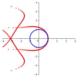
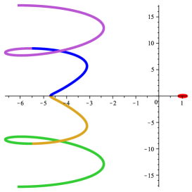
Figure 3: Approximate zeros of the denominator $P(z,e^{\mathbf{i}\theta})$ of $G_{Y}$ inside the rectangular region $[-4-4i,4+4i]$ (left), and the fives curves $\{\rho_{j}(1+0.2e^{\mathbf{i}\theta})\}_{j=-2}^{2}$ for $-\pi\leqslant\theta\leqslant\pi$ (left), where $\rho_{0}$ is the small red circle near unity.

From this approximation and by a direct Taylor expansion of $-(n+1)\log\rho(e^{s})+s+2\log(R_{0}(e^{s}))$ (and justified by the Quasi-Power Framework; see loc. cit.), we obtain the two dominant terms in (22) and (24) (with weaker error terms). Moreover, the same argument applies for higher central cumulants (or moments). In particular, the third and fourth cumulants are asymptotic to

$$\frac{e^{-3}}{8}\left(2e^{2}-17\right)n+c_{3},\quad\text{and}\quad\frac{e^{-4}}{8}\left(-12e^{3}+71\right)n+c_{4},$$

respectively, where ($\phi:=2\Phi(1)-1$)

$$c_{3} =\frac{e^{-3}}{16}\left((2\pi e)^{3/2}\phi^{3}+12\pi e\phi^{2}-\sqrt{2\pi e}\left(4e^{2}-15\right)\phi-64+4e^{2}\right)$$

$$\approx-0.01646\,99733\,69929\dots$$

$$c_{4} =\frac{e^{-4}}{16}\left(-3(e\pi)^{2}\phi^{4}-6(2\pi e)^{3/2}\phi^{3}+2\pi e(4e^{2}-21)\phi^{2}+4\sqrt{2\pi e}\left(4e^{2}-11\right)\phi+280-40e^{2}\right)$$

$$\approx 0.09122\,16766\,24710\dots$$

These expressions show the strength of the Quasi-Power approach. Although the direct approach used in Section 3 to compute the first two moments provides more precise error terms (factorial instead of exponential), the approach used here is computationally simpler, notably for the expressions of the constant terms of high-order central cumulants.

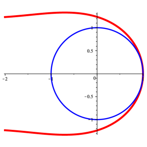
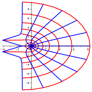
Figure 4: The curve $\rho(t)$ when $|t|=1$ (left), where the unit circle is also shown, and a conformal plot of $\rho(e^{w})$ (right).

For limit and approximation theorems, we are particularly interested in the behavior of the dominant term $\rho(t):=\rho_{0}(t)$ in the asymptotic expansion (35) when $|t|=1$. Note that $\rho(1)=1$ and all other $\rho_{k}(-e^{-1}(1-t)/(1+t))$’s tend to infinity when $t\to 1$. Also

$$\rho_{k}(e^{\mathbf{i}\theta})=e^{-\mathbf{i}\theta}\left(1+W_{k}\left(e^{-1}\frac{\sin\theta}{1+\cos\theta}\,\mathbf{i}\right)\right).$$

From (35), we have, when $|t|=1$

$$X_{n}(t)=tR(t)^{2}\rho(t)^{-n-1}+O\left(4^{-n}\right).$$ (41)

Theorem 3 (Central and local limit theorems).

Let $\mu:=1-e^{-2}/2$ and $\sigma=\sqrt{\frac{3}{4}}\,e^{-1}$. We have

$$\sup_{x\in\mathbb{R}}\left|\mathbb{P}\left(\frac{X_{n}-\mu n}{\sigma\sqrt{n}}\leqslant x\right)-\Phi(x)\right|=O\left(n^{-1/2}\right),$$ (42)

and, uniformly for $x=o(n^{1/6})$,

$$\mathbb{P}\left(X_{n}=\left\lfloor\mu n+x\sigma\sqrt{n}\right\rfloor\right)=\frac{e^{-x^{2}/2}}{\sqrt{2\pi n}\,\sigma}\left(1+O\left((1+|x|^{3})n^{-1/2}\right)\right).$$ (43)

Proof.

(Sketch) The convergence rate (42) follows from (41) and the classical Berry-Esseen inequality, and is part of the Quasi-Power Theorem (see loc. cit.). The local limit theorem is also straightforward by the corresponding Fourier integral representation once we have the uniform bound (41). Details are omitted. ∎

Note that the Berry-Esseen bound (42) with a rate of the form $n^{-1/2+\varepsilon}$ was established in [26]; their formulation is more general but with slightly less precise approximations.

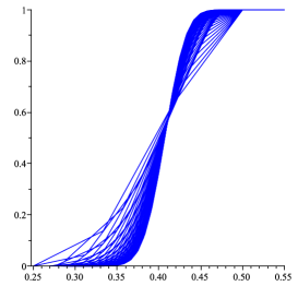
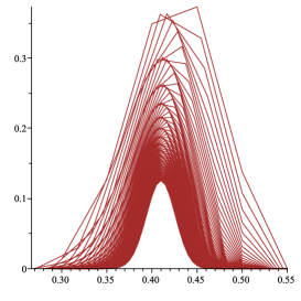
Figure 5: Exact distributions of $X_{n}$ for $n=6,\dots,60$: the distributions are plotted against $1/2n$.

6 Stochastic dominance

We clarify the following stochastic dominance relations in this section.

Theorem 4.

For $n\geqslant 1$

$$A_{n+1},B_{n+1}\geqslant X_{n}\geqslant A_{n-1}-2,B_{n-1}-2,$$ (44)

where we write $X\geqslant Y$ (in distribution) if for all $x$

$$\mathbb{P}(X\leqslant x)\leqslant\mathbb{P}(Y\leqslant x).$$

So the asymptotic normality of $X_{n}$ can be reduced to that of $A_{n}$ and $B_{n}$, which is easier because of the simpler recurrences or the closed-form expressions (19).

The sandwich approximation (44) seems intuitively clear but a rigorous proof is far from being obvious. Our proof given below is simple but messy. On the other hand, the “$-2$” factors in (44) are not optimal and might be replaced by “$-1$”; but our proof is somewhat too weak to justify this.

To prove (44), we establish the following dependence graph of stochastic dominance relations.

(i)

$$\text{(0a) }1+B_{n}\geqslant A_{n},\quad\text{(0b) }1+A_{n}\geqslant B_{n},$$

(ii)

$$\text{(1a) }A_{n}\geqslant A_{n-1},\quad\text{(1b) }B_{n}\geqslant B_{n-1},\quad\text{(1c) }Y_{n}\geqslant Y_{n-1},$$

$$\ \ \text{(2a) }A_{n}\geqslant Y_{n},\ \ \ \quad\text{(2b) }B_{n}\geqslant Y_{n},\quad\ \ \ \text{(2c) }Y_{n}\geqslant X_{n-1},$$

(iii)

$$\text{(3a) }1+B_{n-1}\geqslant A_{n},\quad\ \ \text{(3b) }1+A_{n-1}\geqslant B_{n},\quad\text{(3c) }1+Y_{n-1}\geqslant Y_{n},$$

$$\text{(4a) }1+A_{n-1}\geqslant Y_{n},\quad\ \ \ \text{(4b) }1+B_{n-1}\geqslant Y_{n},\quad\ \ \text{(4c) }1+Y_{n}\geqslant X_{n},$$

(iv)

$$\text{(5a) }1+Y_{n}\geqslant A_{n-1},\quad\ \ \text{(5b) }1+Y_{n}\geqslant B_{n-1},\quad\ \ \text{(5c) }1+X_{n}\geqslant Y_{n}.$$

Combining (2a), (2b) and (2c), we obtain the left-hand side of (44)

$$A_{n},B_{n}\geqslant X_{n-1};$$

on the other hand, combining (5a), (5b) and (5c) leads to

$$2+X_{n}\geqslant A_{n-1},B_{n-1}.$$

which is the right-hand side of (44).

The following directed graph indicates the implications of the diverse stochastic dominance relations. The symbol “A $\rightarrow$ B” means that the proof of B uses the induction hypothesis of A.

Our proof is based on the following properties of conditional probability, which remain true when replacing all “$\geqslant$” by “$\leqslant$”.

Lemma 4.

Assume that $\mathscr{E}_{i}$ are disjoint events of $X$ with $\sum_{i}\mathbb{P}(\mathscr{E}_{i})=1$. If $(X|\mathscr{E}_{i})\geqslant Y$ for all $i$, then $X\geqslant Y$.

Lemma 5.

Assume that $\mathscr{E}_{i},\mathscr{E}_{i}^{\prime}$ are disjoint events of $X,Y$ with $\mathbb{P}(\mathscr{E}_{i})=\mathbb{P}(\mathscr{E}_{i}^{\prime})$ and $\sum_{i}\mathbb{P}(\mathscr{E}_{i})=1$. If $(X|\mathscr{E}_{i})\geqslant(Y|\mathscr{E}_{i}^{\prime})$ for all $i$, then $X\geqslant Y$.

We apply induction for all proofs. The initial conditions in all cases can be readily checked. We assume that all the stochastic dominance relations from (0a) to (5c) hold for all indices up to $n-1$. We will then prove that they also hold when the indices are $n$.

Proof of (0a), (0b).

$1+B_{n}\geqslant A_{n},\ 1+A_{n}\geqslant B_{n}$.

We order each seat with a number from $1$ to $2n$ for $\mathscr{A}_{n}$ and $\mathscr{B}_{n}$ as follows.

and

Let $\mathscr{E}_{i},\mathscr{E}_{i}^{\prime}$ be the events of $A_{n},B_{n}$ in which the first diner occupies seat number $i$. Then

$$(A_{n}|\mathscr{E}_{i})\stackrel{{\scriptstyle d}}{{=}}B_{n-i}+1+A_{i-2},\quad(B_{n}|\mathscr{E}_{i}^{\prime})\stackrel{{\scriptstyle d}}{{=}}A_{n-i}+1+A_{i-2},$$

for $1\leqslant i\leqslant n$,

$$(A_{n}|\mathscr{E}_{i})\stackrel{{\scriptstyle d}}{{=}}A_{n-j-1}+1+B_{j-1},\quad(B_{n}|\mathscr{E}_{i}^{\prime})\stackrel{{\scriptstyle d}}{{=}}B_{n-j-1}+1+B_{j-1},$$

for $i=n+j,1\leqslant j\leqslant n-1$, and

$$(A_{n}|\mathscr{E}_{2n})\stackrel{{\scriptstyle d}}{{=}}1+B_{n-1},\quad(B_{n}|\mathscr{E}_{2n}^{\prime})\stackrel{{\scriptstyle d}}{{=}}1+A_{n-1}.$$

By the induction hypothesis of (0a) and (0b),

$$(1+B_{n}|\mathscr{E}_{i}^{\prime})\geqslant(A_{n}|\mathscr{E}_{i})\quad\text{and}\quad(1+A_{n}|\mathscr{E}_{i})\geqslant(B_{n}|\mathscr{E}_{i}^{\prime})$$

for $1\leqslant i\leqslant 2n$. By Lemma 5, we then prove the two relations $1+B_{n}\geqslant A_{n}$ and $1+A_{n}\geqslant B_{n}$.

Note that the proof uses only relations between $A_{\cdot}$ and $B_{\cdot}$; all other proofs will require the induction hypothesis from other dominance relations.

Proof of (1a), (1b).

$A_{n}\geqslant A_{n-1},B_{n}\geqslant B_{n-1}$.

We first show that $A_{n}\geqslant A_{n-1}$. Let $\mathscr{E}_{1},\mathscr{E}_{2}$ be the events of $A_{n}$ in which the first customer selects seat number $1$ and $2$, respectively. Let $\mathscr{E}_{c}$ be the event of $A_{n}$ in which the first customer selects seat other than numbers $1,2$.

$$\begin{array}[]{cccccccccccc}1&\bigcirc&\bigcirc&\bigcirc&\bigcirc&\bigcirc&\bigcirc&\dots&\bigcirc&\bigcirc&\bigcirc&\\ &2&\bigcirc&\bigcirc&\bigcirc&\bigcirc&\bigcirc&\bigcirc&\cdots&\bigcirc&\bigcirc&\bigcirc\end{array}$$

To apply Lemma 4, we need $(A_{n}|\mathscr{E}_{1}),(A_{n}|\mathscr{E}_{2}),(A_{n}|\mathscr{E}_{c})\geqslant A_{n-1}$. We have

$$(A_{n}|\mathscr{E}_{1})\stackrel{{\scriptstyle d}}{{=}}1+B_{n-1}\geqslant A_{n-1},$$

by the induction hypothesis of (0a), and

$$(A_{n}|\mathscr{E}_{2})\stackrel{{\scriptstyle d}}{{=}}B_{0}+1+A_{n-2}=2+A_{n-2}\geqslant 1+B_{n-1}\geqslant A_{n-1},$$

by the induction hypothesis of (3b) and (0a). Thus $(A_{n}|\mathscr{E}_{1}),(A_{n}|\mathscr{E}_{2})\geqslant A_{n-1}$.

To show that $(A_{n}|\mathscr{E}_{c})\geqslant A_{n-1}$, we consider $(A_{n}|\mathscr{E}_{c})$ and $A_{n-1}$ (defined on the same probability space) and apply Lemma 5. Let $\mathscr{E}_{j}^{\prime}$ be an event of $A_{n-1}$ in which the first customer sits on some seat. Similar to the proof of (0a) and (0b), we see that

$$((A_{n}|\mathscr{E}_{c})|\mathscr{E}_{j}^{\prime})\stackrel{{\scriptstyle d}}{{=}}B_{n-k}+1+A_{k-2}\quad\text{and}\quad(A_{n-1}|\mathscr{E}_{j}^{\prime})\stackrel{{\scriptstyle d}}{{=}}B_{n-k-1}+1+A_{k-2},$$

for some $1\leqslant k\leqslant n-1$, or

$$((A_{n}|\mathscr{E}_{c})|\mathscr{E}_{j}^{\prime})\stackrel{{\scriptstyle d}}{{=}}A_{n-k-1}+1+B_{k-1}\quad\text{and}\quad(A_{n-1}|\mathscr{E}_{j}^{\prime})\stackrel{{\scriptstyle d}}{{=}}A_{n-k-2}+1+B_{k-1},$$

for some $1\leqslant k\leqslant n-1$. By induction hypothesis of (1a) and(1b),

$$((A_{n}|\mathscr{E}_{c})|\mathscr{E}_{j}^{\prime})\geqslant(A_{n-1}|\mathscr{E}_{j}^{\prime})\quad\text{for all }j.$$

By Lemma 5, we obtain $(A_{n}|\mathscr{E}_{c})\geqslant A_{n-1}$. This proves that $A_{n}\geqslant A_{n-1}$. The proof for $B_{n}\geqslant B_{n-1}$ is similar.

The proofs for the other cases follow, mutatis mutandis, the same line of inductive arguments; details are straightforward and omitted here.

7 A combinatorial model

Instead of the sequential stochastic model considered in this paper, more static combinatorial models (sometimes referred to as hard-core mode) were also considered in the literature, where all possible unfriendly seating arrangements are equally likely. Such models turn out to be much simpler to analyze. Let $N_{n}$ denote the total number of distinct unfriendly seating arrangements under the initial configuration $\mathscr{Y}_{n}$ (see (16)). Then $N_{n}$ is given by the Fibonacci number

$$N_{n}=N_{n-1}+N_{n-2}\qquad(n\geqslant 2),$$

with $N_{0}=1$ and $N_{1}=1$. If we still denote by $X_{n}$ and $Y_{n}$ the number of occupied seats when starting with the initial configurations (10) and (16), respectively, as we studied above, then we have the simple recurrences for their probability generating functions

$$X_{n}(t)=tY_{n-1}(t),\quad\text{and}\quad Y_{n}(t)=\frac{tN_{n-1}}{N_{n}}\,Y_{n-1}(t)+\frac{tN_{n-2}}{N_{n}}\,Y_{n-2}(t),$$

with $Y_{0}(t)=1$ and $Y_{1}(t)=t$. This is easily solved and we have

$$X_{n}(t)=\frac{t}{N_{n-1}}\sum_{\left\lceil n/2\right\rceil\leqslant j\leqslant n-1}\binom{j}{n-1-j}t^{j}\qquad(n\geqslant 0),$$

which is the essentially sequences A102426 and A098925 in Sloane’s Encyclopedia of Integer Sequences (see also A092865). This is also connected to the number of parts in random compositions in which only $1$ and $2$ are used. A local limit theorem with optimal convergence rate can be derived by standard means; see [13, IX. 9]. The expected value is asymptotic to $\frac{2}{5-\sqrt{5}}\,n$ and the variance to $\frac{3(3-\sqrt{5})}{\sqrt{5}(5-\sqrt{5})^{2}}\,n$. Numerically, the jamming density is

$$\frac{1}{5-\sqrt{5}}\approx 0.36180\dots,$$

which is smaller than that in the sequential model; the variance constant is much smaller

$$\frac{3(3-\sqrt{5})}{\sqrt{5}(5-\sqrt{5})^{2}}\approx 0.08944\dots.$$

We conclude that the space utilization is better in the sequential model than in the combinatorial model. Such a property has already been observed in the statistical physics literature; see for example [1] (where the combinatorial model is referred to as the Hamiltonian system). Note that for the corresponding 1-row seat configuration, one has the jamming density ($\alpha:=\sqrt[3]{100+12\sqrt{69}}$)

$$\frac{(\alpha-2)(\alpha+2)^{2}(\alpha^{3}-192)}{4416}\approx 0.41149\dots,$$

and the variance constant

$$\frac{6}{529}\cdot\frac{3\alpha^{4}+17\alpha^{3}-184\alpha^{2}+68\alpha+48}{(\alpha^{2}-2\alpha+4)^{2}}\approx 0.008539\dots.$$

See [7, 19] for more information.