Discrete canonical analysis of three dimensional gravity with cosmological constant

Abstract

We discuss the interplay between standard canonical analysis and canonical discretization in three-dimensional gravity with cosmological constant. By using the Hamiltonian analysis, we find that the continuum local symmetries of the theory are given by the on-shell space-time diffeomorphisms, which at the action level, corresponds to the Kalb-Ramond transformations. At the time of discretization, although this symmetry is explicitly broken, we prove that the theory still preserves certain gauge freedom generated by a constant curvature relation in terms of holonomies and the Gauss’s law in the lattice approach.

I INTRODUCTION

The construction of a consistent theory of quantum gravity is a problem in theoretical physics that has so far defied all attempts at resolution. The problem of finding a consistent quantum theory of gravity is in part due to that general relativity is a very complicated mathematical non-linear field theory and furthermore, it’s a geometric theory of spacetime, and quantizing gravity means quantizing spacetime itself, and so far we do not know what this means Kuchar .

In order to overcome such difficulties, it is natural to look for simpler models that share, mathematically and physically, the important conceptual features of general relativity, while avoiding some of the computational difficulties. For quantum gravity, a model as such, is general relativity in three space-time dimensions. As a generally covariant field theory of space-time geometry, $(2+1)$-dimensional gravity possesses the same conceptual foundations as a realistic $(3+1)$-dimensional general relativity, since many of the fundamental issues of quantum gravity carry over to the lower dimensional setting Witten ,Carlip .

For understanding fundamental concepts: the nature of time, the construction of states and observables, the role of topology, and the relationships among different quantization approaches, the model has proven highly instructive Carlip . Classical solutions to the vacuum field equations turn out to be all locally diffeomorphic to spacetimes of constant curvature, that is, Minkowski, de Sitter, or anti-de Sitter spaces. This means that any solution of the field equations with a cosmological constant has constant curvature. Physically, a $(2+1)$-dimensional spacetime has no local degrees of freedom, i.e., there are no gravitational waves in the classical theory, and no propagating gravitons in the quantum theory.

One of the central problems generated by the application of the rules of quantum mechanics to a covariant field theory is the problem of the dynamics. When formulated canonically, general relativity has a vanishing Hamiltonian, which has to be implemented as a constraint. In the loop quantum gravity approach Rovelli , this has been achieved Thiemann , but to characterize the resulting theory in a way in which the dynamics of general relativity is explicit remains a challenge. In order to overpass these obstacles, there has long been the hope that lattice methods could be used as a non-perturbative approach to quantum gravity. This is in part based on the fact that lattice methods had been quite successful in the treatment of quantum chromodynamics (QCD), not only in making the theory finite, but also in making it computable. However, in lattice QCD there exist regularization methods that are gauge invariant, whilst in the gravitational context this is not the case Loll . As soon as one discretizes space-time one breaks the invariance under diffeomorphisms, then lattice methods in the gravitational setting face unique challenges.

To address these problems, it has been proposed a systematic canonical treatment for discretizing covariant field theories, both at a classical and quantum mechanical level. This methodology is related to a discretization technique called variational integrators Marsden , Lew ,Gambini1 ,Gambini2 . This method consists in discretizing the action of the theory and working from it the discrete equations of motion. Automatically, the latter are generically guaranteed to be consistent. The resulting discrete theories have unique features that distinguish them from the continuum theories, although a satisfactory canonical formulation can be found for them. The discrete theories do not have constraints associated with the space-time diffeomorphisms and as a consequence the quantities that in the continuum are the associated Lagrange multipliers become regular variables of the discrete theories whose values are determined by the equations of motion Gambini3 . Furthermore, the discretization breaks the initial gauge freedom and solutions to the discrete theory, that are different correspond, in the continuum limit, to the same solution of the continuum theory. Hence the discrete theory has more degrees of freedom. On the other hand, the lack of constraints makes the discretized theories very promising at the time of quantization, since most of the hard conceptual questions of quantum gravity are related to the presence of constraints in the theory Gambini4 ,Gambini5 .

Considering what is been stated, the purpose of this paper is to present a consistent discretization of $(2+1)$-gravity with cosmological constant, and discuss whether discretization leads to a breaking of the local symmetries of the theory. The organization of the paper is as follows: in section $2$, we study the Kalb-Ramond transformations at the Lagrange level, in section $3$ we develop an extended canonical analysis of the continuum theory by turning the quantities that play the role of Lagrange multipliers into dynamical variables. This extended version, although completely equivalent to the usual one, will allow us to make a cleaner conection with the discrete theory. In section $4$ we briefly review the consistent discretization technique, and in section $5$, we finally discuss $(2+1)$-gravity in a lattice. We end with a discussion and present some conclusions.

II Lagrangian formulation

Let us take the Lie group $SU(2)$ as our gauge group. This group is semisimple so there is an invariant non degenerate bilinear form, the so called, Cartan-Killing form. We take as our spacetime a 3-dimensional oriented smooth manifold $\mathcal{M}$ with $\mathcal{M}=\mathbb{R}\times\Sigma$, right by $\Sigma$ (which we take to be compact and without boundary) corresponding to Cauchy’s surfaces and $\mathbb{R}$ representing an evolution parameter (global hyperbolicity is imposed to exclude spacetimes with bad causality properties). Now choose a principal $SU(2)$-bundle $P$ over $M$. Due to the fact that $SU(2)$ is simply connected, this $SU(2)$-bundle admits a trivialization Baez-bf Cattaneo BF 3-4 dim . We can define the dynamical fields of our theory as follows

• A connection $A$ which is a $su(2)$-valued 1-form on $\mathcal{M}$, $A=A^{\ I}_{\mu}t_{I}dx^{\mu}$.

• A $su(2)$-valued 1-form field $e$ on $\mathcal{M}$, the dreibein, $e=e^{\ I}_{\mu}t_{I}dx^{\mu}$,

where we have defined $t_{I}$, with $I=1,2,3$, as the generators of the $su(2)$ Lie algebra in the adjoint representation. These generators satisfy

$$[t_{I},t_{J}]=2\epsilon_{IJ}^{\ \ \ K}t_{K}$$ (1)

where $\epsilon_{IJK}$ is the totally antisymmetric tensor, Levi-Civita tensor. The Cartan-Killing form is given by

$$\kappa_{IJ}=Tr(t_{I}t_{J})=\delta_{IJ}.$$ (2)

Then, the action principle is given by

$$S\left[e,A\right]=\int_{\mathcal{M}}\ Tr\bigg{[}e\wedge F+\frac{\Lambda}{3}\ e\wedge e\wedge e\bigg{]}=\int_{\mathcal{M}}e_{I}\wedge F^{I}+\frac{\Lambda}{3}\ \epsilon_{IJK}e^{I}\wedge e^{J}\wedge e^{K},$$ (3)

where $\Lambda$ is the cosmological constant and the strength tensor is a $su(2)$-valued 2-form which, as usual, it is taken as $F=dA+A\wedge A$.
The equations of motion from the action read

$$\delta_{A}S=0 \Rightarrow De^{I}=0,$$ (4)

$$\delta_{e}S=0 \Rightarrow F^{I}+\Lambda\ \epsilon^{IJK}e_{J}\wedge e_{K}=0,$$ (5)

where the covariant derivative is defined as, $D\xi^{I}=d\xi^{I}+[A,\xi]^{I}$, for an $su(2)$-valued k-form $\xi^{I}$. The spacetime is locally either flat ($\Lambda=0$), de Sitter ($\Lambda>0$), or anti-de Sitter ($\Lambda<0$).
The equation (4) is the zero-torsion condition, which let us write the connection as function of the dreibein, $A=A(e)$. Then when we use the last result back to the equation of motion (5), we obtain Riemannnian general relativity with cosmological constant Baez-bf , 4-dim BF Functor .
The action, (3), is invariant under $SU(2)$ transformations,

$$\delta_{\alpha}e=[e,\alpha]\qquad\delta_{\alpha}A=D\alpha.$$ (6)

Inspired in the Kalb-Ramond transformation and the transformation of the fields in Horowitz’s theory for the BF model Horowitz ,Broda ,Cattaneo BF 3-4 dim , we find that the action is invariant under field-dependent transformation parameters, defined as

$$\delta_{C}e = DC,$$ (7)

$$\delta_{C}A = \Lambda[C,e],$$ (8)

where $C$ are 0-form $su(2)$-valued transformation parameters. These parameters generate on-shell gauge transformations plus diffeomorphisms of the basic fields. In this manner, if we define the field-dependent parameters as $C^{I}=i_{v}e^{I}=v^{\mu}e^{\ I}_{\mu}$, the Kalb-Ramond transformations read

$$\delta_{v}e^{\ I}_{\nu} = D_{\nu}v^{\mu}\cdot e^{\ I}_{\mu}+v^{\mu}\cdot D_{\nu}e^{\ I}_{\mu},$$ (9)

$$\delta_{v}A^{\ I}_{\nu} = 2v^{\mu}(\Lambda\epsilon^{IJK}e_{\mu J}e_{\nu K}).$$ (10)

Considering the equations of motion (4), (5) and the Bianchi’s identity $DF=0$, we obtain

$$\delta_{v}e = \mathcal{L}_{v}e-\delta_{\alpha}e$$ (11)

$$\delta_{v}A = \mathcal{L}_{v}A-\delta_{\alpha}A$$ (12)

where we have taken the $SU(2)$ field-dependent transformation parameters as, $\alpha^{I}=v^{\rho}A_{\rho}^{\ I}$, and $\mathcal{L}_{v}$ is the usual Lie derivative along the vector field $v$. We can observe that these results coincide with the fact that the previous action, (3), is invariant under diffeomorphisms and internal gauge transformations by construction.
We now turn our attention to develop a canonical analysis of the theory in order to show that the symmetries, we have found in the Lagrangian formalism, are preserved at the Hamiltonian level.

III Canonical Analysis for the three dimensional gravity model

In this section, we carry out an extended canonical analysis of $(2+1)$-gravity; as we mentioned above, this analysis consists in turning the quantities that play the role of Lagrange multipliers into dynamical variables tesis , Berra1 ,Berra2 ,Escalante . This procedure, will allow us to make a cleaner contact with the discrete version, as in order to obtain a consistent discretization, some of the Lagrange multipliers get determined by the scheme, and the evolution is implemented by a canonical transformation, this means that the set of discrete equations that were formely incompatible can be solved simultaneously.

We start from the action (3), taking both $e$ and $A$ as dynamical variables. By performing the $2+1$ decomposition, we can write the action as

$$S\left[e,A\right]=\int_{\mathit{R}\times\Sigma}\eta^{ij}\left[e_{0I}F^{\ \ I}_{ij}-2e_{iI}F_{0j}^{\ \ I}+\Lambda\epsilon_{IJK}e^{\ I}_{0}e^{\ J}_{i}e^{\ K}_{j}\right],$$ (13)

where $\eta^{ij}=\epsilon^{0ij}$. From this action, we identify the Lagrangian density

$$\mathcal{L}=\eta^{ij}\left[e_{0I}F^{\ \ I}_{ij}-2e_{iI}F_{0j}^{\ \ I}+\Lambda\epsilon_{IJK}e^{\ I}_{0}e^{\ J}_{i}e^{\ K}_{j}\right].$$ (14)

By determining the set of dynamical variables, we need the definition of the momenta $\left(p^{\alpha}_{\ A},\pi^{\alpha}_{\ A}\right)$,

$$p^{\alpha}_{\ A}=\frac{\delta\mathcal{L}}{\delta\dot{e}^{\ A}_{\alpha}},\quad\quad\pi^{\alpha}_{\ A}=\frac{\delta\mathcal{L}}{\delta\dot{A}^{\ A}_{\alpha}},$$ (15)

canonically conjugate to $\left(e^{\ A}_{\alpha},A^{\ A}_{\alpha}\right)$. The matrix elements of the Hessian,

$$\frac{\partial^{2}{\mathcal{L}}}{\partial(\partial_{\mu}A_{\alpha}^{\ A})\partial(\partial_{\mu}A_{\beta}^{\ B})},\quad\frac{\partial^{2}{\mathcal{L}}}{\partial(\partial_{\mu}e^{\ A}_{\alpha})\partial(\partial_{\mu}A_{\beta}^{\ B})},\quad\frac{\partial^{2}{\mathcal{L}}}{\partial(\partial_{\mu}e^{\ A}_{\alpha})\partial(\partial_{\mu}e^{\ B}_{\beta})},$$ (16)

vanish, which means that the rank of the Hessian is equal to zero, so that, 18 primary constraints are expected. From the definition of the momenta, it is possible to identify the following 18 primary constraints:

$$\phi^{0}_{\ A} : p^{0}_{\ A}\approx 0,$$

$$\phi^{a}_{\ A} : p^{a}_{\ A}\approx 0,$$

$$\psi^{0}_{\ A} : \pi^{0}_{\ A}\approx 0,$$

$$\psi^{a}_{\ A} : \pi^{a}_{\ A}-2\eta^{ab}e_{bA}\approx 0.$$ (17)

By neglecting the terms on the frontier, the canonical Hamiltonian for the three dimensional gravity model is expressed as

$$H_{\rm c}=-\int_{\Sigma}d^{3}x\ \eta^{ij}\left[-e_{0I}F^{\ \ I}_{ij}-\Lambda\epsilon_{IJK}e^{\ I}_{0}e^{\ J}_{i}e^{\ K}_{j}\right]-A_{0}^{\ I}D_{i}\pi^{i}_{\ I}.$$ (18)

By adding the primary constraints to the canonical Hamiltonian, we obtain the primary Hamiltonian

$$H_{\rm P}=H_{\rm c}+\int_{\Sigma}d^{3}x\left[\lambda_{0}^{\ I}\phi^{0}_{\ I}+\lambda^{\ I}_{i}\phi^{i}_{\ I}+\rho^{\ I}_{0}\psi^{0}_{\ I}+\rho^{\ I}_{i}\psi^{i}_{\ I}\right],$$ (19)

where $\lambda^{\ I}_{0}$, $\lambda^{\ I}_{i}$, $\rho^{\ I}_{0}$ and $\rho^{\ I}_{i}$ are Lagrange multipliers enforcing the constraints. The non-vanishing fundamental Poisson brackets for the theory under study are given by

$$\{e^{\ A}_{\alpha}(x^{0},x),p^{\mu}_{\ I}(y^{0},y)\} = \delta^{\mu}_{\alpha}\delta^{A}_{I}\delta^{2}(x,y),$$

$$\{A^{\ A}_{\alpha}(x^{0},x),\pi^{\mu}_{\ I}(y^{0},y)\} = \delta^{\mu}_{\alpha}\delta^{A}_{I}\delta^{2}(x,y).$$ (20)

Now, we need to identify if the theory has secondary constraints. For this aim, we compute the $18\times 18$ matrix whose entries are the Poisson brackets among the primary constraints

$$\{\phi^{0}_{\ A}(x),\phi^{0}_{\ I}(y)\} = 0,\qquad\{\phi^{a}_{\ A}(x),\phi^{0}_{\ I}(y)\}=0$$

$$\{\phi^{0}_{\ A}(x),\phi^{i}_{\ I}(y)\} = 0,\qquad\{\phi^{a}_{\ A}(x),\phi^{i}_{\ I}(y)\}=0,$$

$$\{\phi^{0}_{\ A}(x),\psi^{0}_{\ I}(y)\} = 0,\qquad\{\phi^{a}_{\ A}(x),\psi^{0}_{\ I}(y)\}=0,$$

$$\{\phi^{0}_{\ A}(x),\psi^{i}_{\ I}(y)\} = 0,\qquad\{\phi^{a}_{\ A}(x),\psi^{i}_{\ I}(y)\}=-2\eta^{ai}\delta_{AI}\delta(x,y),$$

$$\{\psi^{0}_{\ A}(x),\phi^{0}_{\ I}(y)\} = 0,\qquad\{\psi^{a}_{\ A}(x),\phi^{0}_{\ I}(y)\}=0$$

$$\{\psi^{0}_{\ A}(x),\phi^{i}_{\ I}(y)\} = 0,\qquad\{\psi^{a}_{\ A}(x),\phi^{i}_{\ I}(y)\}=-2\eta^{ai}\delta_{AI}\delta(x,y),$$

$$\{\psi^{0}_{\ A}(x),\psi^{0}_{\ I}(y)\} = 0,\qquad\{\psi^{a}_{\ A}(x),\psi^{0}_{\ I}(y)\}=0,$$

$$\{\psi^{0}_{\ A}(x),\psi^{i}_{\ I}(y)\} = 0,\qquad\{\psi^{a}_{\ A}(x),\psi^{i}_{\ I}(y)\}=0.$$

This matrix has rank=12 and 6 linearly independent null-vectors, which implies that there are 6 secondary constraints to be determined by consistency conditions. By requiring consistency of the temporal evolution of the constraints and the 6 null vectors, 6 secondary constraints arise,

$$\dot{\phi}^{0}_{\ A} = \{\phi^{0}_{A},H_{P}\}\approx 0\quad\Rightarrow\quad D^{A}:=\eta^{ab}F_{ab}^{\ \ A}+\Lambda\eta^{bc}\epsilon^{A}_{\;\;BC}e^{\ B}_{b}e^{\ C}_{c}\approx 0,$$

$$\dot{\psi}^{0}_{\ A} = \{\psi^{0}_{A},H_{P}\}\approx 0\quad\Rightarrow\quad G_{A}:=D_{a}\pi^{a}_{\ A}\approx 0,$$ (22)

and the following Lagrange multipliers are fixed,

$$\dot{\phi}^{a}_{\ A} = \{\phi^{a}_{\ A},H_{P}\}\approx 0\quad\Rightarrow\quad\rho_{aA}=-\Lambda\epsilon_{ABC}e^{\ B}_{0}e^{\ C}_{a},$$

$$\dot{\psi}^{a}_{\ A} = \{\psi^{a}_{\ A},H_{P}\}\approx 0\quad\Rightarrow\quad\lambda^{\ A}_{a}=-D_{a}e^{\ A}_{0}+2\epsilon^{A}_{\;\;BC}A^{\ B}_{a}e^{\ C}_{0}-\frac{1}{2}\ \epsilon^{A}_{\;\;BC}A^{\ B}_{0}\pi_{a}^{\ C}.$$ (23)

This theory does not have terciary constraints. By following the method, we determine which of the constraints (primary and secondary) are first class and which are second class. To accomplish such a task we calculate the Poisson brackets between the primary and secondary constraints. To complete the constraint matrix, we add to the algebra shown in Eq. (III) the following expressions

$$\{\phi^{0}_{\ A}(x),G_{I}(y)\} = 0,\qquad\{\phi^{a}_{\ A}(x),G_{I}(y)\}=0$$

$$\{\phi^{0}_{\ A}(x),D^{I}(y)\} = 0,\qquad\{\phi^{a}_{\ A}(x),D^{I}(y)\}=2\Lambda\eta^{ab}\epsilon^{I}_{\ AB}e_{b}^{\ B}\delta(x,y),$$

$$\{\psi^{0}_{\ A}(x),G_{I}(y)\} = 0,\qquad\{\psi^{a}_{\ A}(x),G_{I}(y)\}=\epsilon_{AI}^{\;\;\;\;K}\pi^{a}_{\ K}(y)\delta(x,y)$$

$$\{\psi^{0}_{\ A}(x),D^{I}(y)\} = 0,\qquad\{\psi^{a}_{\ A}(x),D^{I}(y)\}=2\eta^{ai}\left[\delta^{I}_{A}\partial_{i}(y)+\epsilon_{A\;K}^{\;\;\;I}A^{\ K}_{i}(y)\right]\delta(x,y),$$

$$\{D^{A}(x),D^{I}(y)\} = 0,\qquad\{G_{A}(x),D^{I}(y)\}=\epsilon_{A}^{\;\ IC}D_{C}\delta(x,y)=0$$

$$\{G_{A}(x),G_{I}(y)\} = \epsilon_{AI}^{\;\;\;\;C}G_{C}\delta(x,y)=0.$$ (24)

The matrix formed by the Poisson brackets among all the constraints exhibited in Eqs. (III) and (III) has rank=18 and 6 null-vectors. The contraction of the null vectors with the matrix formed by the constraints results in 12 first class constraints:

$$\phi^{0}_{\ A} : p^{0}_{\ A},$$

$$\psi^{0}_{\ A} : \pi^{0}_{\ A},$$

$$G_{A} : D_{a}\pi^{a}_{\ A}+\epsilon_{AB}^{\;\;\;\;\;C}e^{\ B}_{a}p^{a}_{\ C},$$

$$D^{A} : \eta^{ab}F_{ab}^{\ \ A}-\Lambda\eta^{ab}\epsilon^{A}_{\;\;BC}e^{\ B}_{a}e^{\ C}_{b}+\Lambda\epsilon^{A\;C}_{\;B}e^{\ B}_{a}\pi^{a}_{\ C}+D_{a}p^{aA}.$$ (25)

On the other hand, we find 12 second class constraints:

$$\phi^{a}_{\ A} : p^{a}_{\ A},$$

$$\psi^{a}_{\ A} : \pi^{a}_{\ A}-\eta^{ab}e_{bA}.$$ (26)

After this analysis, we conclude the model has 18 canonical variables, 12 independent first class constraints and 12 independent second class constraints, which leads to determine, by performing a counting of the degrees of freedom Henneaux , that this model has none degrees of freedom per space-time point. Of course, by considering the second class constraints Eq. (III) as strong equations, the above relations are reduced to the usual constraints Witten , so that this analysis extends and completes the results in the literature.

By calculating the algebra among the constraints, we find that

$$\{\phi^{0}_{\ A}(x),\phi^{0}_{\ I}(y)\} = 0,\qquad\{\phi^{a}_{\ A}(x),\phi^{i}_{\ I}(y)\}=0,$$

$$\{\phi^{0}_{\ A}(x),\phi^{i}_{\ I}(y)\} = 0,\qquad\{\phi^{a}_{\ A}(x),\psi^{0}_{\ I}(y)\}=0,$$

$$\{\phi^{0}_{\ A}(x),\psi^{0}_{\ I}(y)\} = 0,\qquad\{\phi^{a}_{\ A}(x),\psi^{i}_{\ I}(y)\}=-2\eta^{ai}\delta_{AI}\delta(x,y),$$

$$\{\phi^{0}_{\ A}(x),\psi^{i}_{\ I}(y)\} = 0,\qquad\{\phi^{a}_{\ A}(x),G_{I}(y)\}=\epsilon_{AI}^{\;\;\;\;K}\phi^{a}_{\ K}\delta(x,y),$$

$$\{\phi^{0}_{\ A}(x),G_{I}(y)\} = 0,\qquad\{\phi^{a}_{\ A}(x),D^{I}(y)\}=0,$$

$$\{\phi^{0}_{\ A}(x),D^{I}(y)\} = 0,\qquad\{\psi^{a}_{\ A}(x),\psi^{i}_{\ I}(y)\}=0,$$

$$\{\psi^{0}_{\ A}(x),\psi^{0}_{\ I}(y)\} = 0,\qquad\{\psi^{a}_{\ A}(x),G_{I}(y)\}=\epsilon_{AI}^{\;\;\;\;\;K}\psi^{a}_{\ K}\delta(x,y),$$

$$\{\psi^{0}_{\ A}(x),\psi^{i}_{\ I}(y)\} = 0,\qquad\{\psi^{a}_{\ A}(x),D^{I}(y)\}=\epsilon_{A\;K}^{\;\;\;I}\phi^{a}_{\ K}\delta(x,y),$$

$$\{\psi^{0}_{\ A}(x),G_{I}(y)\} = 0,\qquad\{G_{A}(x),G_{I}(y)\}=\epsilon_{AI}^{\;\;\;\;C}G_{C}\delta(x,y),$$

$$\{\psi^{0}_{\ A}(x),D^{I}(y)\} = 0,\qquad\{G_{A}(x),D^{I}(y)\}=\epsilon_{A\;C}^{\;\;\;I}D^{C}\delta(x,y),$$

$$\{D^{A}(x),D^{I}(y)\} = 0,$$ (27)

from where we can appreciate that the constraints form a set of first and second class constraints, as expected. The determination of the nature of the constraints allow us to find the extended action. By employing the first class constraints, Eq. (III), the second class constraints, Eq. (III), and the Lagrange multipliers, Eq. (III), we find that the extended action takes the form

$$S_{E}[e,p,A,\pi,\lambda,\rho,\gamma,\xi]=\int\left[\dot{e}_{\alpha}^{\ A}p^{\alpha}_{\ A}+\dot{A}_{\alpha}^{\ A}\pi^{\alpha}_{\ A}-H-\lambda_{\alpha}^{\ A}\phi^{\alpha}_{\ A}-\rho^{\ A}_{\alpha}\psi^{\alpha}_{\ A}-\gamma^{A}G_{A}-\xi_{A}D^{A}\right]d^{3}x,$$ (28)

where $H$ is a linear combination of first class constraints, and is given by

$$H=-A_{0}^{\ A}G_{A}-e_{0A}D^{A}$$ (29)

and $\lambda_{\alpha}^{\ A}$ , $\rho_{\alpha}^{\ A}$ , $\gamma^{A}$ , $\xi_{A}$ are the Lagrange multipliers enforcing the first and second class constraints. We observe, by considering the second class constraints as strong equations, that the Hamiltonian shown in Eq. (29) is reduced to the usual expression found in the literature Witten , Carlip , which is defined on a reduced phase space context. From the extended action, we identify the extended Hamiltonian, $H_{\rm E}$, which is given by

$$H_{\rm E}=H-\lambda_{0}^{\ A}\phi^{0}_{\ A}-\rho^{A}_{0}\psi^{0}_{A}-\gamma^{A}G_{A}-\xi_{A}D^{A}.$$ (30)

By utilizing our expressions for the complete set of constraints, it is possible to obtain the gauge transformations acting on the full phase space. For this important step, we shall use the Castellani’s formalism Castellani , which allows us to define the following gauge generator in terms of the first class constraints:

$$G=\int_{\Sigma}\left[D_{0}\varepsilon_{0}^{\ A}\phi^{0}_{A}+D_{0}\zeta_{0}^{\ A}\psi^{0}_{\ I}+\varepsilon^{A}G_{A}+\zeta_{A}D^{A}\right]d^{3}x,$$ (31)

where $\varepsilon_{0}^{\ A}$, $\varepsilon^{\ A}$, $\zeta_{0}^{\ A}$ and $\zeta_{A}$ are arbitrary continuum real parameters. Thus, we find that the gauge transformations in the phase space are

$$\delta_{0}e_{0}^{\ A} = D_{0}\varepsilon_{0}^{\ A},$$

$$\delta_{0}e_{a}^{\ A} = \epsilon^{A}_{\;\;IJ}\varepsilon^{I}e^{\ J}_{a}-D_{a}\zeta^{A},$$

$$\delta_{0}A_{0}^{\ A} = D_{0}\zeta_{0}^{\ A},$$

$$\delta_{0}A_{a}^{\ A} = -D_{a}\varepsilon^{A}+\Lambda\epsilon^{AI}_{\;\;\;J}e^{\ J}_{a},$$

In order to recover the on-shell diffeomorphisms symmetry, one can redefine the gauge parameters as $-\varepsilon_{0}^{\ I}=\varepsilon^{I}=-v^{\alpha}A_{\alpha}^{\ I}$, and $-\zeta^{\ I}_{0}=\zeta^{I}=-v^{\alpha}e_{\alpha}^{\ I}$. By such an election, the gauge tranformations take the form

$$e_{\alpha}^{{}^{\prime}A} \longrightarrow e_{\alpha}^{A}+\mathcal{L}_{v}e^{A}_{\alpha}+\left(v\times De\right)^{\ A}_{\alpha},$$

$$A_{\alpha}^{{}^{\prime}A} \longrightarrow A_{\alpha}^{A}+\mathcal{L}_{v}A^{I}_{\alpha}+\left[v\cdot\left(F+\Lambda e\wedge e\right)\right]^{\ A}_{\alpha}.$$ (33)

Where ”$\times$”, and ”$\cdot$” denote the usual cross and dot product in the three dimensional space-time. By examining the constraints in the complete phase space, we have obtained, in an explicit form, the generators of the gauge transformations for all fields within the action, even if they behave like Lagrange multipliers in accordance with the on-shell Kalb-Ramond transformations found in the last section.

IV Consistent discretization of constrained theories

We illustrate the technique with a mechanical system for simplicity, the case of field theories is straightforward, since upon discretization the latter become mechanical systems Marsden ,Gambini1 ,Gambini2 . We assume we start from an action in the continuum, written in first-order form,

$$S=\int L(q,p)dt,$$ (34)

with

$$L(q,p)=p\dot{q}-H(q,p)-\lambda_{B}\phi^{B}(q,p),$$ (35)

where $\lambda_{B}$ are the Lagrange multipliers that enforce the constraints $\phi^{B}(q,p)=0$. The discretization of the action yields $S=\sum_{n=0}^{N}L(n,n+1)$, where

$$L(n,n+1)=p_{n}(q_{n+1}-q_{n})-\varepsilon H(q_{n},p_{n})-\lambda_{nB}\phi^{B}(q_{n},p_{n}),$$ (36)

where $\varepsilon=t_{n+1}-t_{n}$, and we have absorbed an $\varepsilon$ in the definition of the Lagrange multipliers. In the discrete setting, the Lagrangian can be seen has the generator of a type 1 canonical transformations between the instant $n$ and the instant $n+1$. In order to obtain a fully consistent theory, the equations of the discrete theory must be solved simultaneously, we will view $q_{n}$, $p_{n}$, $\lambda_{nB}$ and $q_{n+1}$, $p_{n+1}$, $\lambda_{n+1B}$ as configuration variables and will assign to each of them a canonically conjugate momentum, $P_{n}^{q}$, $P_{n}^{p}$, $P_{n}^{\lambda_{B}}$ and $P_{n+1}^{q}$, $P_{n+1}^{p}$, $P_{n+1}^{\lambda_{B}}$. If one explicitly computes the partial derivatives with the Lagrangian already given, one can obtain a more familiar-looking set of equations,

$$p_{n}-p_{n-1} = -\varepsilon\frac{\partial H(q_{n},p_{n})}{\partial q_{n}}-\lambda_{nB}\frac{\partial\phi^{B}(q_{n},p_{n})}{\partial q_{n}},$$

$$q_{n+1}-q_{n} = \varepsilon\frac{\partial H(q_{n},p_{n})}{\partial p_{n}}+\lambda_{nB}\frac{\partial\phi^{B}(q_{n},p_{n})}{\partial p_{n}},$$ (37)

$$\phi^{B}(q_{n},p_{n}) = 0.$$

These equations appear very similar to the ones one would obtain by first working out the equations of motion in the continuum and then discretizing them. A significant difference, however, is that when one solves this set of equations some of the Lagrange multipliers get determined, they are not free anymore as they are in the continuum Sigma . We therefore see that generically when one discretizes constrained theories one gets a different structure than in the continuum, in which some of the Lagrange multipliers get undetermined. The equations that in the continuum used to be constraints become upon discretization pseudo-constraints in that they relate variables at different instants of time and are solved by determining the Lagrange multipliers.

V The consistent discretization approach

In this section, we will apply the consistent discretization technique to the three-dimensional gravity with cosmological constant (3), defined on a lattice. We discretize the three dimensional gravity action as follows (see Figure 1),

$$L(n,n+1) =\sum_{v}Tr[e^{0}_{n,v}h^{1}_{n,v}h^{2}_{n,v+e_{1}}(h^{1}_{n,v+e_{2}})^{\dagger}(h^{2}_{n,v})^{\dagger}+e^{2}_{n,v}V_{n,v}h^{1}_{n+1,v}(V_{n,v+e_{1}})^{\dagger}(h^{1}_{n,v})^{\dagger}$$ (38)

$$-e^{1}_{n,v}V_{n,v}h^{2}_{n+1,v}(V_{n,v+e_{2}})^{\dagger}(h^{2}_{n,v})^{\dagger}+\rho_{n,v}(V_{n,v}(V_{n,v})^{\dagger}-1)+\lambda^{1}_{n,v}(h^{1}_{n,v}(h^{1}_{n,v})^{\dagger}-1)$$

$$+\lambda^{2}_{n,v}(h^{2}_{n,v}(h^{2}_{n,v})^{\dagger}-1)+\Lambda\ e^{0}_{n,v}e^{1}_{n,v}e^{2}_{n,v}].$$

By $h^{a}_{n,v}$ we mean the holonomy along the spatial direction of the elementary unit vector $e_{1},e_{2}$, starting from the lattice point labeled by the time step $n$ and the spatial point $v$ (which is labelled by a pair of indices as we are dealing with a three dimensional field theory). By the index $v+e_{a}$, we mean a lattice point coming from the spatial point $v$ in direction of $e_{a}$. The $e$ fields live in a one dimensional surface, dual to the plaquette on which we compute the holonomy representing the curvature field $F$, and hence, it is an element of $SU(2)$, i.e, an algebra valued one form. The symbol $V_{n,v}$ represents the vertical holonomies and are only labelled by the lattice point they start at. We will consider that the holonomies are matrices of the form $h=h^{A}t_{A},V=V^{A}t_{A}$, where $t^{0}=I/\sqrt{2}$ and $t^{I}=-i\sigma^{I}/\sqrt{2}$, and $\sigma^{I}$ are the well known Pauli matrices (In this section, we consider the capital latin letters from the beginning of the alphabet as labels of the gauge group $A,B,\ldots=\{0,I\}$ ). Finally, $\rho$ and $\lambda$ are Lagrange multipliers that enforce, the above defined holonomies are indeed elements of $SU(2)$.

The canonical variables of the theory are $h^{a,A}_{n,v}$, $V_{n,v}^{A}$, $e^{a,I}_{n,v}$, $e^{0,I}_{n,v}$, $\rho_{n,v}$ and $\lambda^{a}_{n,v}$ where $a=1,2$.

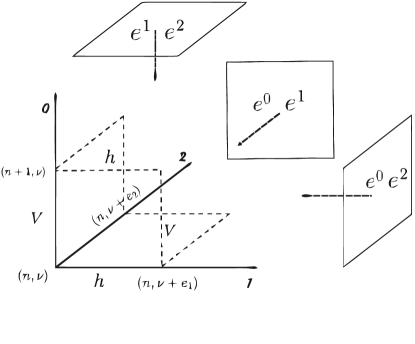
Figure 1: A elementary cell for a discrete description of 2+1 gravity.

The momenta associated for $\lambda^{a}_{n,v}$, are given by

$$\Pi^{\lambda^{a}}_{n+1,v} \equiv \frac{\partial L(n,n+1)}{\partial\lambda^{a}_{n+1,v}}=0,$$

$$\Pi^{\lambda^{a}}_{n,v} \equiv -\frac{\partial L(n,n+1)}{\partial\lambda^{a}_{n,v}}=-Tr\left[h^{a}_{n,v}(h^{a}_{n,v})^{\dagger}-1\right].$$ (39)

Consistency in time leads to the secondary class constraint:

$$Tr\left[h^{a}_{n,v}(h^{a}_{n,v})^{\dagger}-1\right]=0,$$ (40)

which, after time evolution, does not yield any new constraint. The momenta associated for $\rho_{v,n}$, are given by

$$\Pi^{\rho}_{n+1,v} \equiv \frac{\partial L(n,n+1)}{\partial\rho_{n+1,v}}=0,$$

$$\Pi^{\rho}_{n,v} \equiv -\frac{\partial L(n,n+1)}{\partial\rho_{n,v}}=-Tr\left[V_{n,v}(V_{n,v})^{\dagger}-1\right].$$ (41)

Consistency in time leads to the secondary class constraint

$$Tr\left[V_{n,v}(V_{n,v})^{\dagger}-1\right]=0,$$ (42)

which, again is preserved in time without generating any new constraint. Now, we consider the momenta associated to the fields $e^{a}_{n,v}$, which read

$$\Pi^{e^{a}}_{n+1,\nu} \equiv \frac{\partial L(n,n+1)}{\partial e^{a,I}_{n+1,v}}\ (T^{I})^{\dagger}=0,$$

$$\Pi^{e^{a}}_{n,\nu} \equiv -\frac{\partial L(n,n+1)}{\partial e^{a,I}_{n,v}}(T^{I})^{\dagger}=-Tr\left[h^{bc}_{n,v}T_{I}+\Lambda e_{n,v}^{b}e_{n,v}^{c}T_{I}\right](T^{I})^{\dagger},$$ (43)

where $\{a,b,c\}$ represents a cyclic permutation of $\{0,1,2\}$, and $h^{ab}_{n,v}$ stands for an holonomy starting from the point labelled by $n$, $v$, around the elementary plaquette in the plane $a-b$. On the other hand, $e_{n,v}^{a}e_{n,v}^{b}$, is the dual plaquette related to the $a-b$ holonomy, as shown in figure (1). Consistency in time of the constraint (V) leads to

$$Tr\left[h^{ab}_{n,v}T_{I}+\Lambda\ e_{n,v}^{a}e_{n,v}^{b}T_{I}\right]=0,$$ (44)

the most general solution for this equation is given by

$$h^{bc}_{n,v}=-\Lambda\ e^{b}_{n,v}e^{c}_{n,v}+\sigma^{bc}_{n,v}I$$ (45)

where $(h^{bc}_{n,v})^{{\dagger}}=h^{cb}_{n,v}$ and $\sigma^{ab}_{n,v}=\pm 1$, this sign is arbitrary and can change from plaquette to plaquette. The appearance of $\sigma$ is due that the solution is defined upon a traceless termGambini1 .
The expression for the momenta associated with the vertical holonomies, $V_{n,v}^{A}$, are

$$\Pi_{n+1,v}^{V} = \frac{\partial L(n,n+1)}{\partial V_{n+1,v}^{A}}(T^{A})^{\dagger}=0,$$

$$V_{n,v}\Pi_{n,v}^{V} = h^{01}_{n,v}e^{2}_{n,v}-h^{02}_{n,v}e^{1}_{n,v}-(h^{1}_{n,v-e_{1}})^{\dagger}h^{10}_{n,v-e_{1}}e^{2}_{n,v-e_{1}}h^{1}_{n,v-e_{1}}$$ (46)

$$+ (h^{2}_{n,v-e_{2}})^{\dagger}h^{20}_{n,v-e_{2}}e^{1}_{n,v-e_{2}}h^{2}_{n,v-e_{2}}+2\rho_{n,v}I.$$

Preserving in time the constraints (V) , together with (45), we obtain

$$2Tr(-\Lambda e^{0}_{n,v}e^{1}_{n,v}e^{2}_{n,v})+Tr(-\Lambda e^{0}_{n,v-e_{1}}e^{1}_{n,v-e_{1}}e^{2}_{n,v-e_{1}})+Tr(-\Lambda e^{0}_{n,v-e_{2}}e^{1}_{n,v-e_{2}}e^{2}_{n,v-e_{2}})=-4\rho_{n,v},$$ (47)

where we can notice, that all terms are the same three volume element, but evaluated at diferent points. Because the cells are all equivalent and they do not depend on the label attached to them, it is useful to define the trace of the volume element as $\mathcal{V}=Tr(e^{0}_{n,v}e^{1}_{n,v}e^{2}_{n,v})$. Taking this into account, consistency in time of the constraint (V), allow us to fix the multiplier, $\rho_{n,v}=\Lambda\mathcal{V}$. Then, the equation of motion associated to the vertical holonomies, $V_{n,v}$, reads

$$h^{01}_{n,v}e^{2}_{n,v}-h^{02}_{n,v}e^{1}_{n,v}-(h^{1}_{n,v-e_{1}})^{{\dagger}}h^{10}_{n,v-e_{1}}e^{2}_{n,v-e_{1}}h^{1}_{n,v-e_{1}}+(h^{2}_{n,v-e_{2}})^{{\dagger}}h^{20}_{n,v-e_{2}}e^{1}_{n,v-e_{2}}h^{2}_{n,v-e_{2}}=-2\Lambda\mathcal{V}I,$$ (48)

where $I$, denotes the identity matrix. In a similar fashion, and in accordance with the consistent discretization approach, the equation of motion associated to the spatial holonomy, $h^{1}_{n+1,v}$, defined at the point, $(n+1,v)$, is given by

$$h^{1}_{n+1,v}\Pi^{h^{1}}_{n+1,v}=(V_{n,v})^{{\dagger}}h^{01}_{n,v}e^{2}_{n,v}V_{n,v},$$ (49)

by using (45), we obtain the primary constraint

$$Tr(h^{1}_{n+1,v}\Pi^{h^{1}}_{n+1,v})=-\Lambda\mathcal{V}.$$ (50)

Furthermore, the equation of motion associated with the spatial holonomy, $h^{1}_{n,v}$, this time evaluated at the point $(n,v)$, leads to

$$h^{1}_{n,v}\Pi^{h^{1}}_{n,v}=h^{10}_{n,v}e^{2}_{n,v}-h^{12}_{n,v}e^{0}_{n,v}+(h^{2}_{n,v-e_{2}})^{{\dagger}}h^{21}_{n,v-e_{2}}e^{0}_{n,v-e_{2}}h^{2}_{n,v-e_{2}}+2\lambda^{1}_{n,v}I,$$ (51)

preserving in time this contraint, allows us to fix the Lagrange multiplier

$$\lambda^{1}_{n,v}=-\Lambda\mathcal{V}.$$ (52)

We proceed analogously for the variable $h^{2}_{n,v}$. The equation of motion associated with the spatial holonomy $h^{2}_{n+1,v}$, defined at the point $(n+1,v)$ is

$$h^{2}_{n+1,v}\Pi^{h^{2}}_{n+1,v}=-(V_{n,v})^{{\dagger}}h^{02}_{n,v}e^{1}_{n,v}V_{n,v},$$ (53)

from which we obtain the primary constraint

$$Tr(h^{2}_{n+1,v}\Pi^{h^{2}}_{n+1,v})=-\Lambda\mathcal{V},$$ (54)

and the equation of motion related to the spatial holonomy, $h^{2}_{n,v}$, at the point $(n,v)$, gives us

$$h^{2}_{n,v}\Pi^{h^{2}}_{n,v}=h^{21}_{n,v}e^{0}_{n,v}-h^{20}_{n,v}e^{1}_{n,v}-(h^{1}_{n,v-e_{1}})^{{\dagger}}h^{12}_{n,v-e_{1}}e^{0}_{n,v-e_{1}}h^{1}_{n,v-e_{1}}+2\lambda^{2}_{n,v}I,$$ (55)

which fix the corresponding Lagrange multiplier

$$\lambda^{2}_{n,v}=-\Lambda\mathcal{V}.$$ (56)

We now consider the variable, $E^{a}_{n,v}=h^{a}_{n,v}\Pi^{h^{a}}_{n,v}$ with $a\in\{1,2\}$, such combination of spatial holonomies and their associated conjugate momenta, play the role of an electric field, along the direction $e_{a}$ at the point $(n,v)$, in the study of non-abelian theories in the lattice approach. In our case, due to the constraints (50) and (54), we observe that the electric field $E^{a}_{n,v}$, is not an element of the algebra, this occurs because, a closed loop results modified by the presence of the cosmological constant

$$Tr(E^{a}_{n,v})=-\Lambda\mathcal{V}.$$ (57)

For our purposes, it is useful to define the electric field in the opposite direction. $-e_{a}$, evaluated at the point $\{n,v\}$, as

$$E^{\bar{a}}_{n,v}=h^{\bar{a}}_{n,v}\Pi^{h^{\bar{a}}}_{n,v}=(h^{a}_{n,v-e_{a}})^{{\dagger}}(\Pi^{h^{a}}_{n,v-e_{a}})^{{\dagger}}=(h^{a}_{n,v-e_{a}})^{{\dagger}}(E^{a}_{n,v-e_{a}})^{{\dagger}}h^{a}_{n,v-e_{a}}.$$ (58)

In order to calculate $(E^{a}_{n,v})^{\dagger}$, we make use of the following straightforward relations, which can be derived directly from the constraint (45):

$$h^{cb}_{n,v} = h^{bc}_{n,v}+\Lambda\ [e^{b}_{n,v},e^{c}_{n,v}]$$ (59)

$$e^{a}_{n,v}(h^{bc}_{n,v}) = (h^{bc}_{n,v})e^{a}_{n,v}+[e^{a}_{n,v},h^{bc}_{n,v}].$$ (60)

Therefore, the hermitian conjugate of the electric field is given by

$$(E^{a}_{n,v})^{{\dagger}}=-E^{a}_{n,v}+\Lambda\Xi^{a}_{n,v},$$ (61)

where, $\Xi^{a}_{n,v}$, is a linear combination, coming from different permutations of the three-volume element

$$\Xi^{a}_{n,v}=(-1)^{a}\left[e^{1}_{n,v}e^{2}_{n,v}\right]e^{0}_{n,v}+(-1)^{a}\left[e^{1}_{n,v},e^{0}_{n,v}e^{2}_{n,v}\right]+(-1)^{a}\left[e^{0}_{n,v}e^{1}_{n,v},e^{2}_{n,v}\right].$$ (62)

where $a\in\{1,2\}$. With all this at hand, the electric field along the opposite direction, evaluated at point (n,v) reads

$$E^{\bar{a}}_{n,v}=-(h^{a}_{n,v-e_{a}})^{{\dagger}}E^{a}_{n,v-e_{a}}(h^{a}_{n,v-e_{a}})+\Lambda\ (h^{a}_{n,v-e_{a}})^{{\dagger}}\Xi^{a}_{n,v-e_{a}}(h^{a}_{n,v-e_{a}}).$$ (63)

Using the constraints, (45), and the definition of the electric field, one can show that

$$E^{1}_{n+1,v} = +V_{n,v}^{{\dagger}}h^{01}_{n,v}e^{2}_{n,v}V_{n,v}$$ (64)

$$E^{2}_{n+1,v} = -V_{n,v}^{{\dagger}}h^{02}_{n,v}e^{1}_{n,v}V_{n,v}.$$ (65)

Finally, the above relations together with (63), allow us to prove that the equation (48), is equivalent to

$$E^{1}_{n+1,v}+E^{2}_{n+1,v}+E^{\bar{1}}_{n+1,v}+E^{\bar{2}}_{n+1,v}=0$$ (66)

This is, of course, the Gauss’s law defined on the lattice context. When the cosmological constant is present, we observe that the lattice version of $(2+1)$-gravity, preserves a remnant symmetry from the continuum theory, this local discrete symmetry is generated by the internal group thorough the Gauss’s law in its discrete version.
From equation (45), we noted that the holonomy along the spacial plaquettes is proportional to the cosmological constant, which depending on its value we will have (Anti)de Sitter solution or as it was considered at Sigma , flat solutions when the cosmological constant vanishes. But even more, the discrete theory admits more solutions than the continuum one, this is because there is one more term $\sigma^{bc}$ which depends on the plaquettes, in the sense that a possible solution would be a connection that makes the term $\sigma^{bc}$ be +1 on certain plaquettes and -1 on others.
The next step (it will be presented in a future work), will be to solve the discrete constraints as operators on a appropiate Hilbert space, and then construct unitary projectors of the discrete theory onto the physical space of the continuum theory. An useful idea for constructing the physical Hilbert space is to average states in an auxiliary Hilbert space over a suitable action of the gauge group raq1 , raq2 , raq3 . For a noncompact gauge group the averaging need not converge, but when the averaging is formulated within refined algebraic quantisation, convergence on a linear subspace will suffice. Within this formalism, and the nature of the discretization, it is possible to show that the group averaging provides considerable control over quantisation. On the other hand the discretization technique can be viewed as a new paradigm for dealing with cases where the continuum theory does not exist Gambini1 , Sigma .

VI Conclusions

In this paper we have presented a continuous and discrete canonical analysis of the $(2+1)$-dimensional gravity plus cosmological constant. At the lagrangian level we obtained that the gauge invariance generated by the space-time diffeomorphisms is given by the Kalb-Ramond transformations. Then, in order to make a clear-cut comparison with the discrete case, we carried-out an extended canonical analysis of the continuous theory, where all fields were considered as dynamical. Within this context, by examining the constraints in the complete phase space, we obtained in an explicit form, the generators of the gauge transformations for all fields present in the action, even if they behave as Lagrange multipliers, in accordance with the on-shell Kalb-Ramond transformations. Finally, we present a discrete canonical analysis based on the so called variational integrators method. Even though, the discretization breaks the initial gauge freedom, the theory preserves certain gauge invariance generated by the Gauss’s law, but in this case defined on the lattice context. In this manner, a quantisation scheme such as the refined algebraic quantisation will be of wide interest in the treatment of discrete gauge symmetries, whose implications will be the aim future investigations.

Acknowledgements
The authors acknowledges support from a CONACyT scholarship (México), J.E.R.Q. is supported by PROMEP postdoctoral grant.

References

• (1) K. Kuchar, Time and interpretations of quantum gravity, in “Proceedings of the 4th Canadian conference on general relativity and relativistic astro-physics”, G. Kunstatter, D. Vincent, J. Williams (editors), World Scientific, Singapore (1992), C.J. Isham and K.V. Kuchar, Ann. Phys. 164 (1985) 316-333.
• (2) E. Witten, Nucl. Phys. B 311 (1988) 46-78.
• (3) S. Carlip, Phys. Rev. D 42 (1990) 2647-2654.
• (4) A. Ashtekar, J. Lewandowski, Class. Quant. Grav. 21, R53 (2004) [arXiv:gr-qc/0404018],
• (5) Carlo Rovelli, Quantum Gravity, Cambridge University Press, Cambridge, U.K., (2004).
• (6) T. Thiemann, Class. Quan. Grav. 15 839; 875; 1207; 1249; 1281; 1463 (1998).
• (7) R. Loll, Living Rev. Rel. 1, 13 (1998).
• (8) J. Marsden, S. Shkoller, Comm. Math. Phys. 199 351-395 (1985).
• (9) A. Lew, J. Marsden, M. Ortiz,M. West, Finite element methods: 1970’s and beyond, L. Franca, T. Tezduyar, A. Masud, editors, CIMNE, Barcelona (2004).
• (10) C. Di Bartolo, R. Gambini and J. Pullin, Class. Quan. Grav. 19, 5275 (2002) [gr-qc/0205123].
• (11) C. Di Bartolo, R. Gambini,R. Porto and J. Pullin, J. Math. Phys. 46, 012901 (2005) [ gr-qc/0404052].
• (12) C. Di Bartolo, R. Gambini, R. Porto, J. Pullin, J. Math. Phys. 46, 012901 (2005) [gr-qc/0405131].
• (13) R. Gambini, J. Pullin, Gen. Relativity Gravitation 37, 1689–1694 (2005)[gr-qc/0505052].
• (14) M. Campiglia, C. Di Bartolo, R. Gambini, J. Pullin, Phys. Rev. D 74 124012, (2004) [gr-qc/0610023].
• (15) J. Baez, Lect. Notes Phys. 543 25-94, (2009) [gr-qc/9905087v1].
• (16) A. Cattaneo, P. Cotta-Ramusino, J. Fr$\ddot{o}$hlich and M. Martellini, J. Math. Phys. 36 6137-6160, (1995) [hep-th/9505027v2].
• (17) J. Baez, Lett. Math. Phys. 38 129-143, (1996) [arXiv:q-alg/9507006v1].
• (18) G. Horowitz, Commun. Math. Phys. 125 417-437, (1998).
• (19) B. Broda, BF system, Concise Encyclopedia of Supersymmetry And Noncommutative Structures in Mathematics and Physics, Duplij, S.; Siegel, Warren; Bagger, Jonathan (Eds.), (2005) pages 53-54.
• (20) J. Berra, Aplicaciones del formalismo de Dirac-Bergmann estricto a teorías de norma, PhD thesis, FCFM-BUAP, (2012).
• (21) A. Escalante, J. Berra, Int. J. Pure Appl. Math. 79 405-423, (2012) [arXiv:1301.0519].
• (22) A. Escalante, J. Berra, Int. J. Geom. Methods Mod. Phys. 10, 1350030, (2013) [arXiv:1310.3759].
• (23) A. Escalante, L. Carbajal, Annals Phys. 326, 323-339, (2011) [arXiv:1107.4023].
• (24) M. Henneaux, C. Teitelboim, Quantization of Gauge Systems, Princeton Univerity Press (1992).
• (25) L. Castellani, P. van Nieuwenhuizen, M. Pilati, Phys. Rev. D 26 (1982) 352367.
• (26) A. Ashtekar, J. Lewandowski, D Marolf, J. Mourao and T. Thiemann, J. Math. Phys. 36, 6456 (1995).
• (27) D. Giulini, D. Marolf, Class. Quantum Grav. 16, 2489 (1999).
• (28) D. Marolf, Refined algebraic quantization: Systems with a single constraint in: Symplectic Singularities and Geometry of Guague Fields (Banch Center Publications. Polish Academy of Sciences) Warsaw (1997).
• (29) B. Bahr, R. Gambini, J. Pullin, SIGMA 8 (2012), 002, 29 pages [arXiv:1111.1879].