Abstract

We investigate the interference pattern of the charm-resonances $\Psi(3370)$, $\Psi(4040)$, $\Psi(4160)$ and $\Psi(4415)$ with the electroweak penguin operator $O_{9}\propto\bar{b}\gamma_{\alpha}s_{L}\bar{\mu}\gamma^{\alpha}\mu$ in the branching fraction of $B^{+}\to K^{+}\mu\mu$. For this purpose we extract the charm vacuum polarisation via a standard dispersion relation from BESII-data on $e^{+}e^{-}\to{\rm hadrons}$. In the factorisation approximation (FA) the vacuum polarisation describes the interference fully non-perturbatively. The observed interference pattern by the LHCb collaboration is opposite in sign and and significantly enhanced as compared to the FA. A change of the FA-result by a factor of $-2.5$, which correspond to a $350\%$-corrections, results in a reasonable agreement with the data. This raises the question on the size of non-factorisable corrections which are colour enhanced but $\alpha_{s}/(4\pi)$-suppressed. In the parton picture it is found that the corrections are of relative size $\simeq-0.5$ when averaged over the open charm-region which is far below $-3.5$ needed to explain the observed effect. We present combined fits to the BESII- and the LHCb-data, testing for effects beyond the Standard Model (SM)-FA. We cannot find any significant evidence of the parton estimate being too small due to cancellations between the individual resonances. It seems difficult to accommodate the LHCb-result in the standard treatment of the SM or QCD respectively. In the SM the effect can be described in a $q^{2}$-dependent (lepton-pair momentum) shift of the Wilson coefficient combination $C^{\rm eff}_{9}+C^{{}^{\prime}\rm eff}_{9}$. We devise strategies to investigate the microscopic structure in future measurements. For example a determination of $C^{\rm eff}_{9}-C^{{}^{\prime}\rm eff}_{9}$, in the open charm-region, from $B\to K_{\rm longitudinal}^{*}\ell\ell$ or $B\to K_{0}^{*}\ell\ell$ differing from $C^{\rm eff}_{9}+C^{{}^{\prime}\rm eff}_{9}$ implies the presence of right-handed currents and physics beyond the SM. We show that the charm-resonance effects can accommodate the $B\to K^{*}\ell\ell$-anomalies (e.g. $P_{5}^{\prime}$) of the year 2013. Hence our findings indicate that the interpretation of the anomaly through a $Z^{\prime}$-boson, mediating between $bs$ and $\ell\ell$ fields, is disfavoured. More generally our results motivate (re)investigations into $b\to s\bar{c}c$-physics such as the $B\to(\bar{c}c)K^{(*)}$ decays.

I Introduction

We investigate the pronounced resonance-structure found by the LHCb-collaboration LHCb13_resonances in $B^{+}\to K^{+}\ell\ell$ in the open charm-region. The latter corresponds to high lepton pair momentum invariant mass $q^{2}$ (low recoil). In the factorisation approximation (FA), where no gluons are exchanged between the charm-loop and the decaying quarks $b\bar{q}\to s\bar{q}$, the charm-resonance contribution is exactly given by the charm vacuum polarisation. The latter can be extracted, to the precision allowed by the experiment, from the $e^{+}e^{-}\to{\rm hadrons}$ spectrum through first principles by a dispersion relation.

We find that the observed interference pattern has the wrong sign and in addition is more pronounced in the data! Non-factorisable corrections are assessed, following earlier work in the literature, by integrating out the charm quarks and expanding in $1/q^{2}$ for $q^{2}>14\,\mbox{GeV}^{2}$. The relevant contributions (leading to the local resonance structure) are the discontinuities in the amplitude integrated over a suitable duality interval. We find that the integrated effect amounts to a relative correction of $\sim-0.5$. We probe for possible cancelation effects, under the duality integral, by performing combined fits of the BESII- and LHCb-data. Cancellation effects, namely varying phases of the residues of the resonance poles, are not very pronounced. We are led to conclude that our approach to QCD cannot explain the excess of about a factor $\sim-3.5$ with respect to the FA.

In a second part we devise strategies to unravel the microscopic origin of the effect. A promising pathway is to measure the opposite parity combination of Wilson coefficients, that enters $B\to K\ell\ell$, in $B_{(s)}\to K^{*}(\phi)\ell\ell$ or $B\to K_{0}^{*}\ell\ell$ decays for instance. We also show that the effects can explain the $B\to K^{*}\ell\ell$-anomalies, of the year 2013, in the form factor insensitive observable $P_{5}^{\prime}$ below the charmonium threshold.

The paper is organised as follows. In section II we extract the charm vacuum polarisation from BESII-data. The FA in $B\to K\ell\ell$ is assed in section III and in section IV we perform combined fits to the LHCb- and BESII-data. The possible size of non-factorisable corrections are assessed, in some detail, in section V. Strategies to assess the microscopic origin of the effects are presented in section VI. Further it is shown that the effect can easily accommodate the LHCb-anomalies in the low $q^{2}$-region in $B\to K^{*}\ell\ell$. We end with summary and conclusions in section VII.

II Charm vacuum polarisation from BESII-data

We extract the charm vacuum polarisation $h_{c}(s)$ from the BESII data on $e^{+}e^{-}\to\text{hadrons}$. We refer the reader to the textbooks books for reference of the beginning of this section. By virtue of the optical theorem the imaginary part of the vacuum polarisation is related to the experimentally accessible $R$-function

$$R(s)\equiv\frac{\sigma(e^{+}e^{-}\to\text{hadrons})}{\sigma(e^{+}e^{-}\to\mu^{+}\mu^{-})}\;,$$ (1)

as follows

$$\frac{\pi}{3}R_{c}(s)=\frac{1}{2i}{\rm Disc}[h_{c}](s)={\rm Im}[h_{c}](s)\;.$$ (2)

${\rm Disc}[f](s)\equiv f(s+i0)-f(s-i0)$ denotes the discontinuity of the function $f$ at the point $s$. In the case at hand this discontinuity is related to the imaginary part by virtue of the Schwarz reflection principle. The variable $s\equiv q^{2}=E_{\rm cm}^{2}$ denotes the square of centre of mass energy of the $e^{+}e^{-}$-pair. The meaning of the superscript $c$ will be clarified in the next section. The vacuum polarisation $h(s)$ is obtained, through first principles, from the imaginary part (discontinuity) via a once subtracted dispersion relation,

$$h_{c}(s)=h_{c}(s_{0})+\frac{s-s_{0}}{2\pi i}P\int_{{s_{J/\Psi}}}^{\infty}\frac{dt}{t-s_{0}}\frac{{\rm Disc}[h_{c}](t)}{t-s-i0}\;,$$ (3)

where $s_{0}<{s_{J/\Psi}}$ and ${s_{J/\Psi}}=m_{J/\Psi}^{2}-\Delta$ where $\Delta>0$ is sufficiently large such that the tail of $J/\Psi$ is covered. In Eq. (3) $P$ stands for the Cauchy principal part value. The subtraction is necessary in order to regulate the logarithmic ultraviolet UV divergence of the vacuum polarisation. The subtraction constant is fixed by $h(s_{0})$ (which is real) by perturbative QCD to a very good approximation since it is far away from the $J/\Psi$-resonance. In summary given arbitrarily precise data on $R$ one can obtain the vacuum polarisation to arbitrary precision. This is a rather fortunate situation with clear potential for future improvement through more extensive experimental investigation.

II.1 Fitting $R_{c}(s)$ ($3.7\,\mbox{GeV}\leq\sqrt{s}\leq 5\,\mbox{GeV}$) from BESII-data

We redo the fit to the BESII-data ourselves in order to gain control over correlated errors. The uncertainty of the BESII-data is around $6.6\%$ and constitutes a significant improvement over previous experiments which we do not take into consideration. We refer the reader to the particle data group PDG for further reference. Below we describe the separation of the charm part from the light quark flavours, summarise the experimental uncertainties and briefly discuss the fit-model. We stress that in principle the fit-model is not important as far as this work is concerned since we do not aim at extracting resonance parameters such as mass, partial and total widths. Any good fit of the data gives $R_{c}(s)$ and by (3) the full vacuum polarisation. The fit-model is though important as the more realistic it is, the smaller the systematic uncertainty through model-bias.

We denote by $R_{x}$, the $R$-function in a world where the photon exclusively couples to the quark flavour(s) $x$. It is our goal to extract $R_{c}(s)$ since this is the quantity that enters into the factorisable charm contribution in decays of the $B\to K\ell\ell$-type. Neglecting interference between the $u$-, $d$- and $s$- current and the $c$-current implies that $R$ decomposes into $R(s)=R_{uds}(s)+R_{c}(s)$. $R_{uds}(s)$ is well-described by perturbative QCD in the region of interest. E.g. at $E_{\rm cm}=3.782\,\mbox{GeV}$ the theory prediction with uncertainty of about $1\%$ (four loop QCD KST07 ) is consistent with the BESII-data which comes with $~{}5\%$-uncertainty. Moreover $R_{uds}(s)\simeq 2.16$ is quasi-constant over the interval of interest as it is already close to its asymptotic parton-model value of $R_{uds}(s\to\infty)=N_{c}(Q_{u}^{2}+Q_{d}^{2}+Q_{s}^{2})=2$.

The origin of the data and uncertainties necessitate some explanation. The original measurement was published in 2002 in BES02 with statistical and systematic uncertainties as given in table III BES02 . As explained in BES02 the common systematic error is $3.3\%$ which we treat as $100\%$-correlated. The remaining statistical and systematic errors are treated as uncorrelated. In 2008 the BESII collaboration fitted the resonance parameters BES08 which in turn led to changes in the initial state radiation correction and results in slightly shifted values of the $R$-function c.f. Fig.2 BES08 . This shift is taken into account in our analysis.

We take the same fit function as BESII with the exception of the continuum background model for which we choose

$$R_{\rm con}(s)=R_{uds}+(1-z)(\Delta R_{c}+za)\;,\quad\Delta R_{c}\equiv R_{udsc}-R_{uds}\;,$$ (4)

with $z\equiv 4m_{D}^{2}/s$, $R_{uds}=2.16$, $R_{udsc}=3.6$ and $a$ a fit model parameter. The values $R_{uds}$ and $R_{udsc}$ correspond to $R(s_{1}\equiv(3.73\,\mbox{GeV})^{2})$ and $R(s_{2}\equiv(4.8\,\mbox{GeV})^{2})$ where predictions of perturbative QCD and BESII experimental data are in impressive agreement.

The transition amplitudes from resonance $r$ to final state $f$, related to the S-matrix as follows $S=1+i2T$, are modelled by a Breit-Wigner ansatz with energy dependent width and interference effects

$$T^{r\to f}(s)=\frac{m_{r}\sqrt{\Gamma^{r\to e^{+}e^{-}}\Gamma^{r\to f}(s)}}{s-m_{r}^{2}+im_{r}\Gamma_{r}(s)}e^{i\delta_{r}}\;.$$ (5)

The phase $\delta_{r}$ is the phase at the momentum of production of the resonance $r$. The phase due to $f$ does not need to be written since it cancels out in $R(s)$ on grounds of unitarity of the scattering matrix. Only single resonances with quantum numbers of the electromagnetic current ( $J^{\rm PC}=1^{--}$) contribute. In the relevant interval,

$$\text{fit-interval:}\quad 3.7\,\mbox{GeV}\leq\sqrt{s}\leq 5\,\mbox{GeV}\;,$$ (6)

the four $1^{--}$-resonances shown in table 2 are fitted for. The fit parameters are the interference phases $\delta_{r}$, the masses $m_{r}$, the width of the resonance into $e^{+}e^{-}$ as well as one normalisation factor for the width into the final states of $D\bar{D}$-type, based on a model by Eichten et al and experimental data, with appropriate thresholds taken into account. For further details on the modelling of $\Gamma^{r\to f}(s)$, which is rather standard throughout the literature, the reader is referred to the BES-paper BES08 .

$r$	$m_{r}[\,\mbox{GeV}]$	$\Gamma_{r}[\,\mbox{MeV}]$	$\!\!\!\phantom{x}{}^{2s+1}L_{J}$
$J/\Psi$	$3.097$	$0.0934(21)$	$\!\!\!\phantom{x}{}^{3}S_{1}$
$\Psi(2S)$	$3.686$	$0.337(13)$	$\!\!\!\phantom{x}{}^{3}S_{1}$
$\Psi(3370)$	$3.771$	$23.3$	$\!\!\!\phantom{x}{}^{3}D_{1}$
$\Psi(4040)$	$4.039$	$76.2$	$\!\!\!\phantom{x}{}^{3}S_{1}$
$\Psi(4160)$	$4.192$	$73.5$	$\!\!\!\phantom{x}{}^{3}D_{1}$
$\Psi(4415)$	$4.415$	$78.5$	$\!\!\!\phantom{x}{}^{3}S_{1}$

Table 1: $J^{\rm PC}=1^{--}$ charmonium resonances. The first two resonances are narrow and the uncertainties in the masses are negligible PDG . The last four resonances are above the $D\bar{D}$-threshold and as a consequence the width is much larger. We have taken our central fit values from table 5, where more details on the fit can be found. The uncertainty in the widths is considerable.

$r$	$m_{r}[\,\mbox{GeV}]$	$\Gamma_{r}[\,\mbox{MeV}]$
$G(3940)$	$3.943(21)$	$52(11)$
$Y(4008)$	$4.008^{(121)}_{(49)}$	$226(97)$
$Y(4260)$	$4.263(5)$	$108(14)$
$Y(4360)$	$4.353(11)$	$96(42)$

Table 2: $J^{\rm PC}=1^{--}$ exotic (non-charmonium) resonances currently not yet used in the fit. Relevant comments in the main text.

The fit function is given by

$$R_{\rm fit}(s)=R_{\rm res}(s)+R_{\rm con}(s)$$ (7)

with $R_{\rm con}$ as in (4) and the resonance part as given by

$$R_{\rm res}(s)=\frac{9}{\alpha^{2}}\sum_{f}|\sum_{r}T^{r\to f}(s)|^{2}\;.$$ (8)

The factor $9/\alpha^{2}$ comes from the normalisation $\sigma(e^{+}e^{-}\to\mu^{+}\mu^{-})=4\pi\alpha^{2}/(3s)$ where $\alpha$ is the QED fine structure constant. Since only relative phases are observable the first phase $\delta_{\Psi(3370)}\equiv 0$ is set to zero by convention. This amounts to a total number of $(4\times 4-1)_{\rm res}+1_{\rm con}=16$ fit parameters. We perform a $\chi^{2}$ minimisation and obtain a chi squared per degree of freedom (d.o.f.) $\nu=78-16-1=61$ of

$$\chi^{2}/{{\rm d.o.f.}}|_{\rm BESII-data}=1.015$$ (9)

which corresponds to a $p$-value of $44\%$ and is close to $\chi^{2}/{{\rm d.o.f.}}=1.08$ BES08 as should be the case since we employ the same data and a quasi identical model. The fit is shown in Fig. 1 (top) and the fit parameters are given in table 5 in appendix B.1. In agreement with BES08 we observe that $\chi^{2}/{{\rm d.o.f.}}\simeq 1.35$ when the interference phases $\delta_{r}$ are omitted from the ansatz (5).

To this end let us comment on the relevance of exotic charmonium resonances discovered throughout the last decade. The ones of interest for our purposes ($1^{--}$ states that located in the fit-interval) are are listed in table 2 with numbers taken from the review paper HQium-review .

Figure 1: (top) Imaginary part of of vacuum polarisation fitted to BESII data. In the plot we show the BESII error bars with systematic and statistical uncertainty added in quadrature. The $1\sigma$-error band is shown in cyan. (bottom) Real part of the vacuum polarisation obtained from (3) with error band as for the imaginary part.

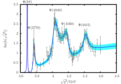
From the viewpoint of the dispersion relation (3), it is immaterial, whether the hadronic model is accurate as long as the fit is good which is measured by the low $\chi^{2}$ (9). It is conceivable that with more data the inclusion of these states would improve the fit. Another possible future improvement would be to extend the Breit-Wigner model into a K-matrix formalism.

II.2 Assembling $R_{c}(s)$ and the vacuum polarisation

The function $R_{c}(s)$ which we fitted in the interval (6) has to be completed below and above the fit-interbal in order to obtain ${\rm Re}[h_{c}]$ through (3). Fortunately this is no problem e.g. KS96a . Below the interval $R_{c}$ is well-approximated by a Breit-Wigner ansatz

$$R_{\text{narrow}}(s)=-\frac{9}{\alpha^{2}}{\rm Im}\Big{[}\sum_{r\in\{J/\Psi,\Psi(2S)\}}\frac{m_{r}\Gamma^{r\to\ell^{+}\ell^{-}}}{s-m_{r}^{2}+im_{r}\Gamma_{r}}\Big{]}\;,$$ (10)

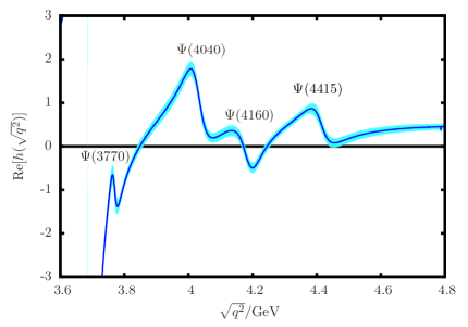
without interference effects since the $J/\Psi$ and $\Psi(2S)$ are narrow and sufficiently far apart from each other. It is noted that (10) relates to (5) through the optical theorem ${\rm Im}[T]=TT^{\dagger}$ when $f=\ell\ell$ and $\delta_{r}\to 0$. Above the fit-interval perturbative QCD provides an excellent approximation. Schwinger’s $O(\alpha_{s})$-interpolation result Schwinger , for $s>4m_{c}^{2}$, reads

$${\rm Im}[h_{c}](s) = {\rm Im}[h_{c}^{(0)}](s)+\alpha_{s}{\rm Im}[h_{c}^{(1)}](s)=\frac{2\pi}{9}(3-v(s)^{2})|v(s)|\Big{(}1+\frac{4}{3}\alpha_{s}\big{(}\frac{\pi}{2v(s)}-\left(\frac{3}{4}+\frac{v(s)}{4}\right)\left(\frac{\pi}{2}-\frac{3}{4\pi}\right)\big{)}\Big{)}\;,$$

where $v(s)\equiv\sqrt{1-4m_{c}^{2}/s}$ is proportional to the charm quark momentum in the centre of mass frame of the lepton pair. The well-known one loop result for real and imaginary part $h^{(0)}$ is given in Eq. (A.12) in the appendix.

III Factorisation gone topsy turvy

III.1 Effective Hamiltonian

In the SM the relevant effective Hamiltonian for $b\to s\ell^{+}\ell^{-}$ transitions reads

$$\mathcal{H}_{\mathrm{eff}}=\frac{G_{F}}{\sqrt{2}}\left(\sum_{i=1}^{2}(\lambda_{u}C_{i}\mathcal{O}_{i}^{u}+\lambda_{c}C_{i}\mathcal{\mathcal{O}}_{i}^{c})-\lambda_{t}\sum_{i=3}^{10}C_{i}\mathcal{O}_{i}\right)\;,\qquad\lambda_{i}\equiv V_{is}^{*}V_{ib}\;,$$ (11)

where the Wilson coefficients $C_{i}(\mu)$ and the operators $O_{i}(\mu)$ carry a dependence on the factorisation scale $\mu$ separating the UV from the infrared (IR) physics. The $b\to s$ unitarity relation reads $\lambda_{u}+\lambda_{c}+\lambda_{t}=0$. For the discussion in this paper we use the basisBuchalla:1995vs

$$\mathcal{O}_{1}^{q} =(\bar{s}_{i}q_{j})_{V-A}(\bar{q}_{j}b_{i})_{V-A} \mathcal{O}_{2}^{q} =(\bar{s}_{i}q_{i})_{V-A}(\bar{q}_{j}b_{j})_{V-A}$$

$$\mathcal{O}_{3} =(\bar{s}_{i}b_{i})_{V-A}\sum_{q}(\bar{q}_{j}q_{j})_{V-A} \mathcal{O}_{4} =(\bar{s}_{i}b_{j})_{V-A}\sum_{q}(\bar{q}_{j}q_{i})_{V-A}$$

$$\mathcal{O}_{5} =(\bar{s}_{i}b_{i})_{V-A}\sum_{q}(\bar{q}_{j}q_{j})_{V+A} \mathcal{O}_{6} =(\bar{s}_{i}b_{j})_{V-A}\sum_{q}(\bar{q}_{j}q_{i})_{V+A}$$

$$\mathcal{O}_{7} =-\frac{em_{b}}{8\pi^{2}}\bar{s}\sigma\cdot F(1+\gamma_{5})b \mathcal{O}_{8} =-\frac{g_{s}m_{b}}{8\pi^{2}}\bar{s}\sigma\cdot G(1+\gamma_{5})b$$

$$\mathcal{O}_{9} =\frac{\alpha}{2\pi}(\bar{\ell}\gamma^{\mu}\ell)(\bar{s}\gamma_{\mu}(1-\gamma_{5})b) \mathcal{O}_{10} =\frac{\alpha}{2\pi}(\bar{\ell}\gamma^{\mu}\gamma_{5}\ell)(\bar{s}\gamma_{\mu}(1-\gamma_{5})b)\;,$$ (12)

where $i,j$ are colour indices, $(\bar{s}b)_{V\pm A}=\bar{s}\gamma^{\mu}(1\pm\gamma_{5})b$, $e=\sqrt{4\pi\alpha}>0$ and $G_{F}$ is the Fermi constant.

Figure 2: Numerically leading contributions to the decay rate of $B\to K\ell\ell$ in the high $q^{2}$-region. (a) and (b) $O_{7}$ and $O_{9,10}$ short distance contributions. These contributions are proportional to the local (short distance) form factors. (c) long distance charm-loop contribution which in (naive) factorisation is proportional to the same form factor times the charm vacuum polarisation $h_{c}(q^{2})$. The charm bubble itself is the full non-perturbative vacuum polarisation since it is extracted directly from the data.

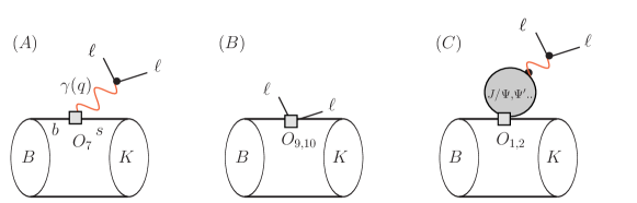
At high $q^{2}$, by which we mean above the narrow charmonium resonances, the numerically most relevant contributions to $B\to K\ell\ell$ are given by the form factor contributions $\mathcal{O}_{7}$ and $\mathcal{O}_{9,10}$ (c.f. Fig. 2AB as well as the tree-level four quark operators $\mathcal{O}^{c}_{1,2}$ which have sizeable Wilson coefficients.) In this section we employ the (naive) factorisation approximation (FA) for which,

$$\langle K|C_{1}\mathcal{O}_{1}^{c}+C_{2}\mathcal{O}_{2}^{c}|B\rangle|_{\rm FA}\propto(C_{1}+C_{2}/3)f^{B\to K}_{+}(q^{2})h_{c}(q^{2})\;,$$ (13)

the matrix element factorises into the charm vacuum polarisation $h_{c}$ times the short distance form factor as defined in Eq. (A.1). This contribution has got the same form factor dependence as $C_{9}$ and can therefore be absorbed into an effective Wilson coefficient $C_{9}^{\mathrm{eff}}$ (A.9) and (A.10). The combination $C_{1}+C_{2}/3$ is known as the “colour suppressed" combination of Wilson coefficients because of a substantial cancellation of the two Wilson coefficients (c.f. appendix A.3). This point will be addressed when we discuss the estimate of the ${\cal O}(\alpha_{s})$-corrections.

III.2 SM-$B\to K\ell\ell$ in factorisation

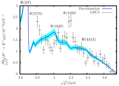
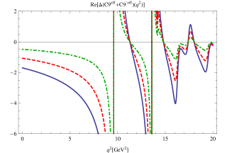
Our SM prediction with lattice form factors Lattice13 (c.f. appendix A.2 for more details), for the $B\to K\ell\ell$-rate are shown in Fig. 3 against the LHCb data LHCb13_resonances ; merci . It is apparent to the eye that the resonance effects, in (naive) factorisation, turn out to have the wrong sign! Not only that but they also seem more pronounced in the data which will be reflected in the fits to be described below.

Figure 3: $B\to K\ell\ell$ rate for high $E\equiv\sqrt{q^{2}}$ just above the $\Psi(3770)$-resonance up to the kinematic endpoint. The $40$ LHCb bins LHCb13_resonances ; merci are shown with grey crosses. The solid blue line corresponds to our SM prediction using FA (the non-factorisable corrections are discussed in chapter V). The cyan band is the theory error band. The mismatch between FA and the data is apparent to the eye.

IV Combined fits to BESII and LHCb data in and beyond factorisation

Before addressing the relevant issue of corrections to the SM-FA in section V, we present a series combined fits to the BESII and LHCb-data. We first describe the fit models before commenting on the results towards the end of the section. The number of fit parameters and the number of d.o.f., denoted by $\nu$, are given in brackets below. We take $78$ BESII data points and $39$ LHCb bins, excluding the last bin which has a negative entry, amounting to a total of $117$ data points.

• Normalisation of the rate, ($17=1_{{\eta_{\cal B}}}+16_{\rm res}$ fit-parameter ${\eta_{\cal B}}$, $\nu=117-17-1=99$)
  In the FA the normalisation of the rate is given by the form factors $f_{+,T}(q^{2})$. Since the latter are closely related in the high $q^{2}$-region by Isgur-Wise relation this amounts effectively to an overall normalisation. To be precise we parameterise the pre-factor, inserted into (A.1) with $m_{l}=0$ for the sake of illustration, as follows

  $$\frac{d\Gamma}{dq^{2}}^{B\to K\ell^{+}\ell^{-}}\propto\quad{\eta_{\cal B}}(|H^{V}|^{2}+|H^{A}|^{2})\;,$$ (14)

  where $V$ and $A$ refer to the lepton polarisation.

• Prefactor of $h_{c}(q^{2})$, ($18=2_{{\eta_{\cal B}},{\eta_{c}}}+16_{\rm res}$ fit parameters, $\nu=117-18-1=98$)
  In addition to the normalisation, we fit for a scale factor ${\eta_{c}}$ in front of the factorisable charm-loop $h_{c}(q^{2})$. More precisely:

  $$H^{V}=C_{9}^{\rm eff}\frac{(m_{B}+m_{K})}{2m_{b}}f_{+}(q^{2})+C_{7}^{\rm eff}f_{T}(q^{2})\;,$$

  $$C_{9}^{\rm eff}=(C_{9}+{\eta_{c}}a_{\rm{\rm fac}}h_{c}(q^{2})+...)$$ (15)

  where $C_{9}(\mu)\simeq 4$, $C_{7}^{\rm eff}(\mu)\simeq-0.3$, $a_{\rm{\rm fac}}(\mu)\simeq 0.6$ at $\mu\simeq m_{b}$ and $h_{c}(q^{2})$ is shown in Fig. 1. The dots stand for quark loops of other flavours.

In a next step we probe for non-factorisable corrections by letting the fit residues of the LHCb data take on arbitrary real (fit-c) and complex (fit-d) numbers. We would like to emphasise that in addition to non-factorisable effects new operators with $J^{PC}[\bar{c}\Gamma c]=1^{--}$, other than the vector current, can also lead to such effects. More discussion can be found later on.

For the charm vacuum polarisation the discontinuity ${\rm Disc}[h_{c}]$ is necessarily positive Eq. (8,2) and its relation to physical quantities is given (5). Hence we can test for physics beyond SM FA by the following replacement

$$|\sum_{r}T^{r\to f}(s)|^{2}\to(\sum_{r}\rho_{r}T^{r\to f}(s))(\sum_{r}T^{r\to f}(s))^{*}\;.$$ (16)

The scale factor $\rho_{r}$ roughly corresponds to ${\cal A}(B\to K\Psi)/f^{B\to K}_{+}(q^{2})$ and replaces ${\cal A}(\Psi\to\ell\ell)$ in (5).

For the fits c) and d) we are not going to put any background model to the LHCb-fit since with the current precision of the LHCb data it seems difficult to crosscheck for the correctness of any model. The background is essentially zero at the $\bar{D}D$-threshold and is expected to raise smoothly with kinks at the thresholds of various $D\bar{D}$-thresholds (with the two $D$’s being any of $D,D^{*},D_{s},D^{*},D_{1},\dots$) into the region where perturbation theory becomes accurate. In fact this is the essence behind the model ansatz (4). The branching fraction has just got the opposite behaviour to the background and this is the reason why it seems difficult to extract the background from the data. More data could, of course, improve the situation.

• Variable residues $\rho_{r}\in\mathbb{R}$, ($22=1_{{\eta_{\cal B}}}+5_{\rho_{r}}+16_{\rm res}$ fit parameters, $\nu=117-32-1=94$)
  We choose to keep ${\eta_{\cal B}}\equiv 1$ and parameterise $\rho_{\Psi(2S)}$ instead which is an equivalent procedure. The five parameters $\rho_{r}$ are constrained to be real.

• Variable residues $\rho_{r}\in\mathbb{C}$, ($27=1_{{\eta_{\cal B}}}+10_{\rho_{r}}+16_{\rm res}$ fit parameters, $\nu=117-27-1=89$)
  Idem but with $\rho_{r}\in\mathbb{C}$ allowing for dynamical phases, therefore introducing 5 new fit parameters.

Figure 4: LHCb-data LHCb13_resonances ; merci (grey crosses) versus the fits b) c) d) described in the main text.

The fits are shown in Fig. 4 and the values are given in table 3. Some more detail on the fit-procedure is described in appendix B.2. Below we comment on each of the fits.

• If the FA was a good approximation then the fit on the first line indicates that that the SM is excluded by a $p$-value of $\simeq 10^{-30}$. This is much more significant than $5\sigma$ (see appendix B.2 for a refined remark).

• Allowing for the charm-resonance prefactor ${\eta_{c}}$ to vary gives a (reasonable) $\chi^{2}$ per degree of freedom with a $p$-value of about $2.1\%$. Most noticeably ${\eta_{c}}=-2.55$ is rather large and negative. The nominal value of non-factorisable corrections correspond to a shift of $\Delta{\eta_{c}}\simeq-0.5$ and hence ${\eta_{c}}=-2.55$ would indicate an effect which is seven times larger. This statement is to be refined under fits c) and d) and the discussion in the next section.

• It is noticeable that there is no uniformity in the residues which in principle is a sign for contributions beyond the SM-FA. Yet there are two important points we would like to make, First the $\chi^{2}/$d.o.f.$\simeq 1.17$ and $1.12$ cannot be seen as a drastic improvement over $\chi^{2}/{\rm d.o.f.}_{\rm fit\;b)}\simeq 1.33$ and hence it is not clear how much one can read into these fits. Second the residues of $\Psi(2S)$ and $\Psi(3370)$ cannot be taken at face value since they essentially have opposite magnitude in fits c) and d). Yet, as can be inferred from plots in Fig. 4, the curves are hardly distinguishable in the relevant region. This is an issue that could be improved with further data points below $\sqrt{q^{2}}=3.770\,\mbox{GeV}$. On average the last three residues reflect the ${\eta_{\cal B}}=-2.55$ shift seen in fit-b).

Fit	${\eta_{\cal B}}$	${\eta_{c}}$	$\rho_{\Psi(2S)}$	$\rho_{\Psi(3370)}$	$\rho_{\Psi(4040)}$	$\rho_{\Psi(4160)}$	$\rho_{\Psi(4415)}$	$\chi^{2}/$d.o.f.	d.o.f.	pts	$p$-value
$a)$	$0.98$	$\equiv 1$	$\equiv 1$	$\equiv 1$	$\equiv 1$	$\equiv 1$	$\equiv 1$	$3.59$	$99$	$117$	$\simeq 10^{-30}$
$b)$	$1.08$	-$2.55$	$\equiv 1$	$\equiv 1$	$\equiv 1$	$\equiv 1$	$\equiv 1$	$1.334$	$98$	$117$	$1.5\%$
$c)$	$0.81$	$\equiv 1$	-$1.3$	-$7.2$	-$1.9$	-$4.6$	-$3.0$	$1.169$	$94$	$117$	$12\%$
$d)$	$1.06$	$\equiv 1$	$3.8$-$5.1i$	-$0.1$-$2.3i$	-$0.5$-$1.2i$	-$3.0$-$3.1i$	-$4.5$+$2.3i$	$1.124$	$89$	$117$	$20\%$
			$6.4e^{-i53.3^{\circ}}$	$2.0e^{-i92^{\circ}}$	$1.3e^{-i111^{\circ}}$	$4.3e^{-i135^{\circ}}$	$5.1e^{i153^{\circ}}$

Table 3: Combined fit to BESII and LHCb-data. The parameter ${\eta_{\cal B}}$ (14) is an overall normalisation factor, (b)) is the pre coefficient of $h_{c}(q^{2})$ and the meaning of $\rho_{\Psi}$ is given in (16). The prediction for the SM-FA is $({\eta_{\cal B}},{\eta_{c}},\rho_{\Psi})=(1,1,1)$. For fit-d) we have given the residues in cartesian polar complex coordinates. The background-model fit-parameter $a$ (4) for fits a) to d) is given by $a=(2.886,2.655,3.100,3.056)$ respectively. As explained in the text the background model is not applied to fits c) and d).

V Discussion on non-factorisable corrections

The size of non-factorisable corrections in $b\to s\bar{c}c$-transitions is a recurring question since the latter are not colour suppressed (c.f. appendix A.3 for a brief discussion) as opposed to the factorisable corrections. This raises the question of whether or not the non-factorisable contribution, being $\alpha_{s}$ suppressed, could dominate as a result of the colour enhancement (or colour non-suppression). Our investigation indicates that this is unlikely to be the case for $B\to K\ell\ell$ for $q^{2}>s_{D\!\bar{D}}$.

The section is organised as follows. First the sizeable corrections are identified in subsection V.1. In subsection V.2 the topic under investigation is elaborated on from the viewpoint of a dispersion relation, (non)-positivity and Breit-Wigner resonances. Finally the size of the correction are estimated through the partonic picture and through the actual data in subsections V.3 and V.4. This section consists of a lengthy, but important, chain of arguments. The casual reader might want to directly pass to the final message in subsection V.5.

V.1 Integrating out the charm quarks

To go beyond the FA, in the parton picture, one gluon exchanges between the charm-loop and the $B\to K$-transition need to assessed. This is a difficult task in principle. In the kinematic situation $q^{2}$ constitutes, fortunately, a large scale that can be taken advantage of by integrating out the virtual charm quarks in the loop. Using the external field method $\bar{b}D^{n}s$-operators, in increasing dimension ($3+n)$, are generated. The symbol $D^{n}$ represents $n$ covariant derivatives. This approach was suggested and investigated in GP04 within heavy quark effective theory. An analysis in QCD (without expanding in the $m_{b}$-mass) including modelling of duality violation effects was given in BBF11 . This framework has become known as the “high-$q^{2}$ operator product expansion (OPE)". The term OPE is a bit derived in the sense above since strictly speaking an OPE is a short distance expansion whereas the resonance region corresponds to a regime where hadrons propagate over long distances. Hence, unlike in the previous section we can not hope to resolve the corrections locally in $q^{2}$ (as shown in the plot in Fig. 3). Yet one can get an estimate of the effect on the helicity amplitudes by integrating over suitable, to be made more precise, duality intervals. It is this quantity that we compare to the FA integrated over the same interval.

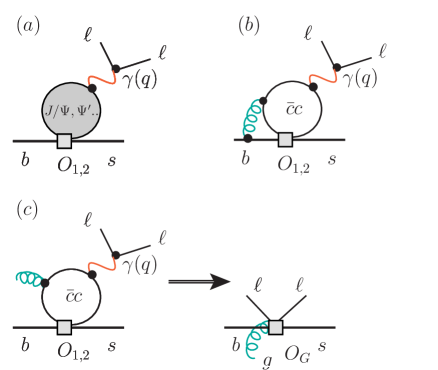
The correlation function that contributes to the helicity amplitude $H^{V}$ (b)) is given by

$$\Gamma_{\mu}=\sum_{k}C_{k}\int d^{4}xe^{iq\cdot x}\langle K(p)|Tj_{\mu}^{\rm em}(x)\mathcal{O}_{k}(0)|B(p_{B})\rangle=Q_{c}\Gamma^{(c)}_{\mu}+Q_{s}\Gamma^{(s)}_{\mu}+Q_{b}\Gamma^{(b)}_{\mu}\;,$$ (17)

where $\mathcal{O}_{k}$ is one of the four quark operators in (III.1) and $j_{\mu}^{\rm em}$ is the electromagnetic operator. In this work we are only interested in effects that contribute to a single resonant structure in the $\bar{c}c$-channel. Hence we restrict our attention to the electromagnetic charm current contribution $\Gamma^{(c)}_{\mu}$. Three typical contributions to $\Gamma^{(c)}_{\mu}$ are indicated in Fig. 5. Fig. 5a corresponds to the FA studied in section III. The contributions in Fig. 5bc are the kind of contributions whose size we intend to assess in this section.

To do so we extend $C_{7,9}^{\rm eff}$ to include the correction from GPS08

$$C_{9}^{\rm eff}=C_{9}+\delta C_{9}^{\rm{\rm fac}}+\delta C_{9}^{\rm{\rm cor}},\quad C_{7}^{\rm eff}=C_{7}+\delta C_{7}^{\rm{\rm cor}}\;,$$ (18)

where $\delta C_{9}^{\rm{\rm fac}}=a_{\rm{\rm fac}}h_{c}(q^{2})$ (Fig. 5a) was implicitly given in (b)) and $\delta C_{7}^{\rm{\rm fac}}=0$. The non-factorisable contributions (Figs.5bc) are denoted by $\delta C_{7,9}^{\rm{\rm cor}}$. The correction to Fig. 5b is given by $\delta C_{7,9}^{\rm{\rm cor}}|_{\rm Fig.\ref{fig:OPEc}b}=-\frac{\alpha_{s}}{4\pi}(C_{1}F_{1}^{(7,9)}(q^{2})+C_{2}F_{2}^{(7,9)}(q^{2}))-\alpha_{s}a_{\rm{\rm fac}}h_{c}^{(1)}$. We have subtracted the $\alpha_{s}$-corrections $h^{(1)}_{c}$ from the result $F_{i}^{j}$ given in GPS08 . The contribution $h^{(1)}$ corresponds to fig1e in GPS08 . In order to compare the relative size we introduce the ratio

$$x(s)=\frac{H^{V,{\rm cor}}(s)}{H^{V,{\rm fac}}(s)}=\frac{\delta C_{9}^{{\rm cor}}(s)+\delta C_{7}^{{\rm cor}}(s)\varphi(s)}{a_{\rm{\rm fac}}h_{c}(s)}\;.$$ (19)

The function $\varphi(s)=(2m_{b}f_{T}(s))/((m_{B}+m_{K})f_{+}(s))$ is the quotient of the $C_{7,9}^{\rm eff}$-prefactors in (b)) and is close to unity and slowly varying. Ideally we would like to know the function $x(q^{2})$ through the high $q^{2}$-region in which case we would simply incorporate it into the results. As emphasised above we cannot hope to do that since $H^{V,{\rm cor}}(s)$ only makes sense when integrated over a suitable (duality) interval.

Figure 5: Contributions to high-$q^{2}$ OPE. (a) dimension $3$ factorisable correction (b) dimension $3$ example of ${\cal O}(\alpha_{s})$-correction (c) dimension $5$ operator shown with loop and contracted loop.

• Diagram Fig 5B: vertex corrections
  These have been evaluated for the inclusive decay $b\to s\ell\ell$, in the high $q^{2}$-region, numerically GIHY03 and analytically GPS08 , in a well-converging expansion in $m_{c}^{2}/m_{b}^{2}$. Using the work of GPS08 ; merci2 we were able to extract the $\Gamma^{(c)}$-contribution. The subtraction of $h^{(1)}$ as described above leads to a sizeable enhancement of $H^{V,{\rm cor},b}$ at $\mu=m_{b}$. It is found that $|x(s)|\simeq 0.5$. Hence this contribution is sizeable. In section V.3 this estimate will be tested against cancellation effects under the duality integral.

• Diagram Fig 5C: $\bar{b}Gs$-corrections
  The correction in Fig. 5c results in a dimension five matrix element of the form $\langle K|\bar{s}_{L}\gamma_{\lambda}gG_{\alpha\beta}b|B\rangle/q^{2}f(4m_{c}^{2}/q^{2})$ with appropriate contractions of kinematical factors. The function $f$ originates from the charm-loop and has a form similar to $h^{(0)}_{c}(q^{2})$ (A.12) in leading order perturbation theory.

  The remaining gluon can either connect to the spectator $H^{V,\rm spec}$, the $K$-meson $H^{V,gK}$ or the $B$-meson $H^{V,gB}$. The first case has been evaluated in BBF11 within QCD factorisation. Comparing the latter with $H^{V,{\rm fac}}(q^{2}>s_{D\!\bar{D}})$ translates into $|x|_{Fig.~{}\ref{fig:OPEc}c}^{\rm spec}\simeq 0.02$. Even though QCD factorisation can only give a rough estimate in the region, as emphasised by the authors of BBF11 , this strongly indicates that this type of correction is negligible; especially as compared to the vertex corrections. Note this is also consistent with the hard spectator scattering contributions in Beneke:2001at being roughly $4\%$ (at $q^{2}=8\,\mbox{GeV}^{2}$) as compared to the leading order contributions. We have evaluated $H^{V,gK}$ in light-cone sum rules at $q^{2}\simeq s_{D\!\bar{D}}$ and find LZ14b $|x|_{Fig.~{}\ref{fig:OPEc}c}^{\rm gK}\simeq 0.02$. The contribution $H^{V,gB}$ has been assessed in KMPW10 in the low $q^{2}$-region and comparing with MXZ08 it is found that $|H^{V,gB}(0)|\simeq 2|H^{V,gK^{*}}(0)|$ which indicates that this contribution is negligible as well. We wish to emphasise that it might be worthwhile to check the size of the different contributions in one framework at $O(\alpha_{s})$ rather than gathering results from three different approaches.

In summary we have identified the vertex corrections Fig. 5b as the main source of corrections. Since we are really interested in the local $q^{2}$-behaviour of the corrections we need to go further and address the question in the hadron picture through quark hadron duality.

V.2 Dispersion relations, (non)-positivity and quark hadron duality

The canonical approach to quark hadron duality is based on dispersion relations e.g. PQW ; Shifman which follow from first principles. Dispersion relations are well established at the amplitude level and in essence just require knowledge of the analytic structure on the physical sheet. We assume that the helicity amplitude $H^{V,{\rm cor}}(q^{2})$ has the same analytic structure as $H^{V,{\rm fac}}(q^{2})$ ($h_{c}$ respectively) and therefore obeys the same dispersion relation (3)

$$H^{V,X}(s)=H^{V,X}(s_{0})+\frac{(s-s_{0})}{2\pi i}\int_{{s_{J/\Psi}}}^{\infty}\frac{dt}{t-s_{0}}\frac{{\rm Disc}[H^{V,X}](t)}{t-s-i0}\;,\quad X\in\{{\rm fac},{\rm cor}\}\;.$$ (20)

The local behaviour of $H^{V,X}(q^{2})$ near a resonance $r$ is well approximated by a Breit-Wigner resonance

$$H^{V,X}(q^{2}\simeq m_{r}^{2})\simeq\frac{-r^{X}_{r}}{q^{2}-m_{r}^{2}+im_{r}\Gamma_{r}}+..\;,$$ (21)

where we shall refer to $r^{X}_{r}$ as the residue. A first important point is that

$$r_{r}^{{\rm fac}} = a_{\rm{\rm fac}}\frac{3\pi}{\alpha^{2}}\Gamma^{r\to\ell\ell}m_{r}>0\;,\quad$$

$$r_{r}^{{\rm cor}} \in \mathbb{C}\;.$$ (22)

For $r_{r}^{\rm fac}$ we have quoted the result of the Breit-Wigner approximation. Positivity of ${\rm Disc}[H^{V,{\rm fac}}]/(2i)={\rm Im}[H^{V,{\rm fac}}]$ follows on more general grounds. First from the positivity of the cross section $R_{c}(s)>0$. Second from the positivity of the Källén-Lehmann spectral representation of a diagonal two point function. For $r_{r}^{{\rm cor}}$ there is no such constraint and $r_{r}^{{\rm cor}}$ is generally a complex number (as in fit-d) where the phase is associated with the scattering phase of the corresponding amplitudes (c.f. footnote 13). Hence the major pitfall we have to be concerned with is that due to non-positivity of the $r_{r}^{{\rm cor}}$ (or ${\rm Disc}[H^{V,{\rm cor}}]/(2\pi i))$ a global dispersion integral might majorly underestimate local or semi-local effects. The fact that all the residues in fit-c) come out with the same sign suggests that this is presumably not the case. On the other hand fit-d) indicates that there could be cancellations to some degree as the phase varies (mildly) as a function of $q^{2}$. For this reason we have to further pursue our investigation with some care and detail.

V.2.1 Intervals of duality in $B\to K\ell\ell$

Using that below the thresholds

$$H^{V,X}(s)^{\rm QCD}\simeq H^{V,X}(s)^{\rm pQCD}\;,\quad s\ll 4m_{c}^{2}\;,$$ (23)

fixes the problem of the subtraction point (20). Global quark hadron duality in (23,3) translates into

$$\langle{\rm Disc}[H^{V,X}]^{\rm QCD}\rangle_{\bar{\omega}}^{({s_{J/\Psi}},\infty)}\simeq\langle{\rm Disc}[H^{V,X}]^{\rm pQCD}\rangle_{\bar{\omega}}^{(4m_{c}^{2},\infty)}$$ (24)

provided the weighting function

$$\bar{\omega}(t)\equiv\frac{1}{(t-s_{0})(t-s-i0)}$$ (25)

is used under the integral average

$$\langle f\rangle^{(s_{1},s_{2})}_{\omega}\equiv\int_{s_{1}}^{s_{2}}dt\omega(t)f(t)\;.$$ (26)

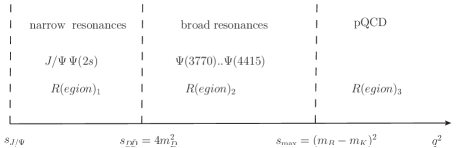
Relation Eq. (24) is precise up to the order $\alpha_{s}$ to which the right hand side is computed in perturbation theory. It is self understood that the variables $s$ and $s_{0}$ are sufficiently far away from the discontinuities. The crucial question, known as semi-global quark hadron duality e.g. Shifman , is then to what degree this equation still holds when the integration interval is split up into different regions. For our purposes the discussion naturally splits into three regions shown in Fig. 7: the lowest interval from $s_{J/\Psi}$ to the $D\bar{D}$-threshold $s_{D\!\bar{D}}\equiv 4m_{D}^{2}\simeq(3.73\,\mbox{GeV})^{2}$ (including the two narrow resonances $J/\Psi$ and $\Psi(2S)$), the interval therefrom to the kinematic endpoint $s_{\rm max}\equiv(m_{B}-m_{K})^{2}\simeq(4.75\,\mbox{GeV})^{2}$ and the third interval extending to infinity. We shall denote those three regions by $R_{1,2,3}$ respectively. In the interval $R_{3}$, not accessible in $B\to K$, the resonances are very broad and smoothly become a part of the continuum. This region is well described by perturbative QCD even locally. This can be inferred from the comparison with the BESII-data for ${\rm Disc}H^{V,{\rm fac}}$ KST07 . It therefore follows that

$$\langle{\rm Disc}[H^{V,X}]^{\rm QCD}\rangle_{\bar{\omega}}^{({s_{J/\Psi}},s_{\rm max})}\simeq\langle{\rm Disc}[H^{V,X}]^{\rm pQCD}\rangle_{\bar{\omega}}^{(4m_{c}^{2},s_{\rm max})}\;,$$ (27)

is a reasonable approximation (semi-global quark hadron duality). Whereas the local description of the narrow resonance region $R_{1}$ is particularly hopeless, the same is not true of the region $R_{2}$ where the $D\bar{D}$-threshold renders the resonances sufficiently broad such that perturbation theory becomes valid on average. This is at least true for ${\rm Disc}H^{V,{\rm fac}}=a_{\rm{\rm fac}}h_{c}$, as can be inferred from the plots of Fig. 6 or the equivalent plots of the $R$-function in PDG . Hence one ought to expect that

$$\langle{\rm Disc}[H^{V,X}]^{\rm QCD}\rangle_{\bar{\omega}}^{(s_{D\!\bar{D}},s_{\rm max})}\simeq\langle{\rm Disc}[H^{V,X}]^{\rm pQCD}\rangle_{\bar{\omega}}^{(s_{D\!\bar{D}},s_{\rm max})}$$ (28)

holds approximately. Eqs.  (24,27,28) are expected to hold for smooth smearing function $\omega$, other than $\bar{\omega}$ (25) PQW . For example for the penguin amplitude it interferes with in $B\to K\ell\ell$. Relation (28) is the basis of further investigations. We shall use (28) to put the previous quoted estimate $|x|\simeq 0.5$ on more solid grounds. In a second step apply it directly to the extracted fits to the LHCb-data.

Figure 6: Plots of the real (straight purple line) and imaginary part (dashed blue line) of the perturbative QCD $h^{(0)}$-function (thin lines) and the QCD $h_{c}$ (thick lines) as fitted from BES data. The latter are shown in Fig. 1. ${\rm Re}[h_{c}^{(0)}]$ is obtained through the dispersion integral (3).

Figure 7: Three regions in $q^{2}$, relevant to the charm-resonances: narrow resonance region which cannot be described by perturbative QCD (left), broad resonance region, of interest to this work, described by perturbative QCD on average (middle) and the third region which is even locally described by perturbative QCD (right).

V.3 The size of the SM vertex corrections over duality interval

The residue version of factorisable versus non-factorisable contribution (19) is given by

$$x_{r}=(\rho_{r}-1)=\frac{r_{r}^{{\rm cor}}}{r_{r}^{{\rm fac}}}\simeq\left.x_{D}(s)\right|_{s\simeq m_{r}^{2}}\;.$$ (29)

where

$$x_{D}(s)\equiv\frac{{\rm Disc}[H^{V,{\rm cor}}](s)}{{\rm Disc}[H^{V,{\rm fac}}](s)}\;.$$ (30)

The quantity $x_{D}$ is an improved version of $x$ (19) since it is does not depend on the subtraction constant for example which is immaterial to the shape in the region of interest. The contribution of the FA is given by ${\rm Disc}[H^{V,{\rm fac}}](s)=2i{\rm Im}[H^{V,{\rm fac}}](s)$ (2), whereas the function ${\rm Disc}[H^{V,{\rm cor},b}](s)$ does not obey such a simple relation since there are cuts below the charm threshold ${\rm Im}[H^{V,{\rm cor},b}]_{q^{2}<4m_{c}^{2}}\neq 0$. For example cuts in the variable $m_{b}^{2}\geq(2m_{c}+m_{s})^{2}$ in Fig. 1c in GPS08 . Using the results in AACW01 one can verify that ${\rm Im}[H^{V,{\rm cor},b}](4m_{c}^{2}-\Delta)/{\rm Im}[H^{V,{\rm cor},b}](4m_{c}^{2}+\Delta)$ (for $0<\Delta<2\,\mbox{GeV}^{2}$) is a very small quantity and hence those cuts are negligible in the region where $q^{2}>4m_{c}^{2}$. Hence we conclude that

$${\rm Disc}[H^{V,{\rm cor},b}](s)\simeq 2i{\rm Im}[H^{V,{\rm cor},b}](s)$$ (31)

is a good approximation. Once more we emphasise that only the vertex corrections proportional to $Q_{c}$ are to be considered. The procedure for obtaining them has been outlined under the first item in section V.1. The quantity $x_{D}^{b}\simeq-0.5$ throughout the relevant interval $s_{D\!\bar{D}}<q^{2}<s_{\rm max}$ for $\mu=4\,\mbox{GeV}$ and only slightly higher values for $\mu=2\,\mbox{GeV}$ as can be inferred from Fig. 13 in appendix A.4. The optimal choice of scale $\mu=m_{b}$, aimed at maximising the effect of the BESII-data, is discussed in appendix A.4. Hence the size of the vertex correction integrated over $R_{2}$ (c.f. Fig. 7) is approximately given by

$$(x_{D})^{\rm SM}_{R_{2}}=\frac{\langle{\rm Disc}[H^{V,{\rm cor}}]^{\rm QCD}\rangle^{(s_{D\!\bar{D}},s_{\rm max})}}{\langle{\rm Disc}[H^{V,{\rm fac}}]^{\rm QCD}\rangle^{(s_{D\!\bar{D}},s_{\rm max})}}\stackrel{{\scriptstyle\eqref{eq:d3}}}{{\simeq}}\frac{\langle{\rm Disc}[H^{V,{\rm cor}}]^{\rm pQCD}\rangle^{(s_{D\!\bar{D}},s_{\rm max})}}{\langle{\rm Disc}[H^{V,{\rm fac}}]^{\rm pQCD}\rangle^{(s_{D\!\bar{D}},s_{\rm max})}}\simeq-0.5\;,$$ (32)

for any reasonably smooth smearing function $\omega$. The last equality follows from the fact that $x_{D}(s)$ is nearly constant throughout the region $R_{2}$. This is estimate puts the previous estimate $|x|\simeq 0.5$ on more solid grounds and settles the effect of the sign in a more definite way. As previously mentioned a correction of $-0.5$ (32) is down by a factor of seven.

V.4 The local and semi-global charmonium excess over FA from LHCb-data

In this subsection we perform a similar analysis as before but comparing the actual discontinuity of the amplitudes that we extract from the fit. We would like to test whether (non)-positivity can lead to effects that are underestimated in duality integrals. An important aspect is that the fits c) and d) do not contain a background model, a problem we have commented on in section IV, and hence we can only extract the resonant contribution. The background is expected to be smooth and does therefore not influence the resonant shape in any significant way.

Hence the discontinuity of the resonant part beyond FA, as extracted from the fit, is given by

$${\rm Disc}[\delta H_{\rm res}^{V,\rm fit}]={\rm Disc}[H_{\rm res}^{V,\rm fit}]-{\rm Disc}[H_{\rm res}^{V,{\rm fac}}]\;,$$ (33)

where

$${\rm Disc}[H_{\rm res}^{V,{\rm fac}}]=a_{\rm{\rm fac}}\frac{6\pi i}{\alpha^{2}}\sum_{f}|\sum_{r}T^{r\to f}|^{2}\;,$$ (34)

$${\rm Disc}[H_{\rm res}^{V,\rm fit}]=a_{\rm{\rm fac}}\frac{6\pi i}{\alpha^{2}}\sum_{f}(\sum_{r}\rho_{r}T^{r\to f}(s))(\sum_{r}T^{r\to f}(s))^{*}\;,$$ (35)

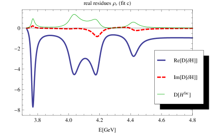
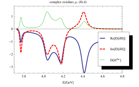
follow from Eqs. (1,2) and Eq. (16) respectively. Note that ${\rm Disc}[H_{\rm res}^{V,\rm fit}]$ is generally not real, even for real $\rho_{r}$. Plots of the various quantities, which can be reconstructed from the fit-data in table 3, are given in Fig. 8. For the fit-c) there are no significant signs of cancellation effects whereas for the fit-d) we can see that the imaginary part does cancel to some extent when integrated over the interval as an effect of the approximately $90^{\circ}$ phase shift between the residues $\rho_{\Psi(4160)}$ and $\rho_{\Psi(4415)}$. This shift might not be a solid feature since the model, in that region, does not result in a very good fit of the LHCb rate (c.f. Fig. 4). Finally we perform the averages of the duality interval to find

$$(x_{D})^{\rm res-data}_{R_{2}}=\frac{\langle{\rm Disc}[\delta H^{V,\rm fit}_{\rm res}]\rangle^{(s_{\rm th},s_{\rm max})}_{\omega=1}}{\langle{\rm Disc}[H_{\rm res}^{V,{\rm fac}}]\rangle^{(s_{\rm th},s_{\rm max})}_{\omega=1}}\simeq\begin{cases}4.0e^{-i176^{\circ}}\simeq 3.2e^{-i176^{\circ}}[\eta_{{\cal B},c}^{-1}]&\text{fit-c)}\\[2.84544pt] 2.5e^{-i152^{\circ}}\simeq 2.7e^{-i152^{\circ}}[\eta_{{\cal B},d}^{-1}]&\text{fit-d)}\end{cases}\;.$$ (36)

The numbers are robust under change of smooth smearing function, for example for $\omega(q^{2})=1/(q^{2}(q^{2}+8\,\mbox{GeV}^{2}))$ we get $4.1e^{-i177^{\circ}}$ and $2.5e^{-i147^{\circ}}$ for fit-c) and -d) respectively. The global scaling factor ${\eta_{\cal B}}$ (14) refers to the number in table 3 which has to be taken into account when comparing numbers between different fits. We observe a shift from $3.2$ to $2.5$ due to complex residues which is what one would expect by inspecting the graphs in Fig. 8. This corresponds to an effect below $25\%$ and can not be seen as very significant. The numbers $3.2[\eta_{{\cal B},c}^{-1}]$ and $2.5[\eta_{{\cal B},d}^{-1}]$ have to be compared with $|{\eta_{c}}-1|\simeq 3.5[\eta_{{\cal B},b}^{-1}]$ and are a bit but not really significantly lower. One has to keep in mind that, for fits-c) and -d), no background model has been used to fit the LHCb-data as previously explained. In this sense the relative closeness of the results of fit-c) and fit-d) are more important than the relative closeness to fit-b).

Figure 8: Plots of fits c) (top) and d) (bottom) with real and complex residues. The abbreviation in the plots stand for the following shorthands ${\rm Re}[D[\delta H]]+i{\rm Im}[D[\delta H]]=2ia_{\rm{\rm fac}}{\rm Disc}[\delta H_{\rm res}^{V,\rm fit}]$ (33) (thick blue and red dashed line for imaginary and real part) and $=D[H_{\rm res}^{\rm fac}]=2ia_{\rm{\rm fac}}{\rm Disc}[H_{\rm res}^{V,{\rm fac}}]$ (thin green line) with $a_{\rm{\rm fac}}(m_{b})\simeq 0.6$. The plots are a direct reflection of the fit-data given in table 3.

V.5 Summary of assessment of non-factorisable corrections

In assessing the non-factorisable contributions in the SM model we have made use of the large scale $q^{2}\geq s_{D\!\bar{D}}$ by integrating out the charm quarks. The vertex corrections in Fig. 5c were identified as sizeable. The relative size of corrections were found to be $-0.5$ with respect to the factorisable corrections when integrated over the duality region $R_{2}=[s_{D\!\bar{D}},s_{\rm max}]$. This is substantially below -$3.5$ as suggested by fit-b) in table 3. The conclusion remained robust under fits c) and d) when the residues were allowed to depart from the ratios dictated by the FA. The data does not suggest major cancellations, due to non-positivity of the duality integrand, in the case of complex residues c.f. (36). In our assessment we have not found any signs of sources within the SM that could give rise to such large corrections.

VI Consequences, strategies and speculations on the origin of the charmonium anomalies

In the previous section we have analysed whether or not the $B\to K\ell\ell$ charm-resonances can be accommodated within the dimension six effective Hamiltonian (11), commonly used to describe $b\to s\ell\ell$-transitions. We have found no indications that this is the case with current understanding. In subsection VI.1 we propose strategies to measure the effect in other $b\to s\ell\ell$ observables and or transitions. One of the main goals being to extract the opposite parity Wilson coefficient combination. In subsection VI.2 we investigate the connection to the $B\to K^{*}\ell\ell$-anomalies of the year 2013. This is not an obvious task since we do not have any precise knowledge of the microscopic effect that leads to the anomalous resonance behaviour. Finally in subsection VI.3 we briefly entertain speculations beyond the SM. The essence of the discussion is summarised in subsection VI.4.

VI.1 Strategies to disentangle the microscopic origin of the charm-resonance anomalies

First we note that, on grounds of parity, the $B\to K\ell\ell$-transition couples to the vector current and therefore to the $C_{+}\equiv C+C^{\prime}$-Wilson coefficient combination. Assuming that the $\ell\ell$-pair emerges through a photon the effect can be absorbed into the $C^{\rm eff}_{9+}\equiv C_{9}^{\rm eff}+C_{9}^{\rm eff}$ Wilson coefficient combination.

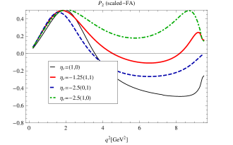
In order to assess the nature of the effect we are going to use fit-b) in table 3 as a template and simply scale the factorisable part by factors of ${\eta_{c}}$. We shall refer to this type as the ${\eta_{c}}$ scaled-FA. The effect on $C^{\rm eff}_{9+}$ is shown for real and imaginary part in Fig. 9. There are several reasons why we choose fit-b) over fits c) and d). First for fit-b) we, at least, have a microscopic (effective) theory at hand whereas for the other two fits this is not the case. In addition, and of course related, for fits c) and d) we did not incorporate a background model and a subtraction constant. As previously mentioned the drop in $\chi^{2}$ is not overwhelming c.f. Tab. 3 and this underlines the importance of the first remark. One has to keep in mind that only one observable, namely the high-$q^{2}$ $B\to K\ell\ell$-rate, was fitted for. With future data the situation would improve considerably. First one could hope to fit for a background model and a (real) subtraction constant in (27). Second the plethora of observables in $b\to s\ell\ell$ constrain the ${\rm Disc}[H^{V,X}]$ in (27) more severely. In essence the plots in this section should be seen as an illustration of the effect and we therefore, al least in this version, do not give uncertainties for the predictions. Yet the ${\eta_{c}}=(1,0)$ case corresponds to the SM-FA and can be discriminated against future experimental data.

Figure 9: Real and imaginary part of $\Delta C_{9}^{\rm eff}(q^{2})$ ($C_{9}^{\rm eff}(q^{2})\equiv C_{9}^{\rm eff,SM}(q^{2})+\Delta C_{9}^{\rm eff}(q^{2})$) for different values of ${\eta_{\cal B}}=-2.5,-1.2,0$. The value ${\eta_{c}}=-2.5$ corresponds to the fit-b) in section IV.

We list a few remarks relevant to $B\to K\ell\ell$ and $B\to K^{*}\ell\ell$ (and or $B_{s}\to\phi\ell\ell$). First $B\to K\ell\ell$:

• $C_{9+}$ decreases the $B\to K\ell\ell$ branching fraction in the low and high $q^{2}$-region which is in qualitative accordance with the recent LHCb analysis with larger binning $3{\rm fb}^{-1}$LHCb14Iso . For high $q^{2}$ this is of course only consistent with the finer binning result elaborated on in this work. For low $q^{2}$ the decrease arises through the decrease of $C_{9+}$.

• The shift of $C_{9+}$ on average is of the same order as demanded by the $P_{5}^{\prime}$-anomaly understanding ; AS13 ; latticepheno ; Beaujean:2013soa . There is though an important qualitative difference in that the shift, suggested by our work, is $q^{2}$-dependent rather than a uniform shift understanding ; AS13 ; latticepheno ; Beaujean:2013soa . More comments can be found in subsection VI.2.

• The two other angular observables in $B\to K\ell\ell$ (due to the opening angle of the lepton-pair), $F_{H}$ and $A_{\rm FB}$ are proportional to effects of ${\cal O}(m_{l})$ in the SM; e.g. BHP07 . It therefore seems, currently, difficult to extract sensible information in our framework. The LHCb-data at $3{\rm fb}^{-1}$LHCbBKllang is consistent with the tiny SM predictions. The two observables are of course of importance to set bounds on new physics operators.

For $B\to K^{*}\ell\ell$ matters are more complex which makes predictions in a first instance more complicated but in the long term allows to disentangle microscopic features of the interactions.

• Combination of Wilson coefficients
  Whereas $B\to K\ell\ell$ probes $C_{9+}$, in $B\to K^{*}\ell\ell$ both combinations $C_{9\pm}$ enter the decay rate, depending on the parity properties of the helicity amplitudes (e.g. HZ13 ),

  $$H_{\perp}\sim C_{9+}\;,\quad H_{0,\parallel}\sim C_{9-}\;.$$ (37)

  We will parameterise the effect, extending the parameterisation (b)), as follows

  $$C_{9}^{\rm eff}=(C_{9}+\eta_{c}a_{\rm{\rm fac}}h_{c}(q^{2})+...)\;,\quad C_{9}^{{}^{\prime}\rm eff}=(C^{\prime}_{9}+\eta^{\prime}_{c}a_{\rm{\rm fac}}h_{c}(q^{2})+...)\;,\quad{\eta_{c}}|_{K}\to(\eta_{c}+\eta^{\prime}_{c})_{K^{*}}\;.$$ (38)

  Hence with information from $B\to K\ell\ell$ only there is ambiguity in predicting $B\to K^{*}\ell\ell$. Conversely this ambiguity can be resolved with the aid of $B\to K^{*}\ell\ell$-observables. To get an idea of the qualitative nature of the effect we choose the following three scenarios:

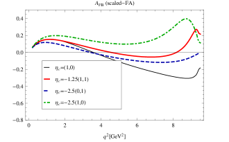
  $$(i)\;{\eta_{c}}\equiv(\eta_{c},\eta^{\prime}_{c})=-1.25(1,1)\;,\quad(ii)\;{\eta_{c}}=-2.5(0,1)\;,\quad(iii)\;{\eta_{c}}=-2.5(1,0)\;.$$ (39)

  An important general strategy is to find observables which are sensitive to $C_{9-}$. A sizeable difference in $C_{9+}-C_{9-}=2C_{9^{\prime}}$ is a direct sign of the presence of right-handed currents and structure beyond the SM.

  

  

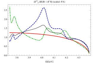
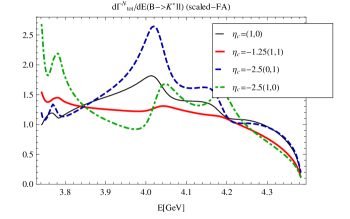
  Figure 10: Plots of the longitudinal and total decay rate in the high $q^{2}$ region for different values of ${\eta_{c}}=(\eta_{c},\eta^{\prime}_{c})$ in the scaled-FA. The normalisation is such that $d\Gamma^{N}/dq^{2}(q^{2}=14\,\mbox{GeV}^{2})=1$ for ${\eta_{c}}=(1,0)$. The plots are useful to distinguish between the three scenarios (39). Comments on the computation are the same as in the caption of Fig.11. The crossing of all four curves, just below the point $15\,\mbox{GeV}^{2}$ originates from $\Delta(C_{9}^{\rm eff}+C_{9}^{{}^{\prime}\rm eff})=0$ going through zero at the same point c.f. Fig. 9. The real part interpolates between a dip and a peak through zero and the imaginary part goes to zero since the resonances $\Psi(3370)$ and $\Psi(4040)$ are spaced widely enough from each other.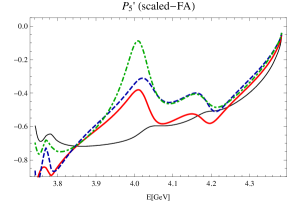

  

  

  

  

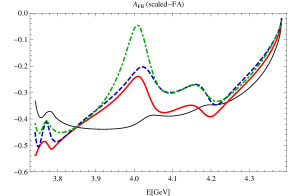
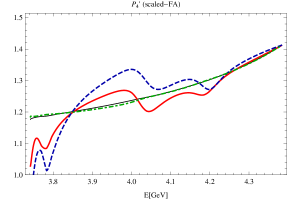
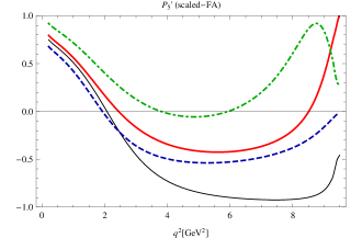
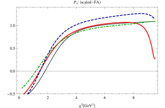
  Figure 11: Plots of $P_{5}^{\prime}$, $A_{\rm FB}$, $P_{4}^{\prime}$ and $F_{L}$ for different values of ${\eta_{c}}=(\eta_{c},\eta^{\prime}_{c})$ in the scaled-FA. The observables $P_{4}^{\prime}$ and $F_{L}$, in the ${\eta_{c}}$-scaled FA , are insensitive to changes in $\eta_{c}$ but sensitive to changes in $\eta^{\prime}_{c}$ and therefore right-handed currents. The exact endpoint predictions HZ13 are $P_{5}^{\prime}(s_{\rm max})=0$, $A_{\rm FB}(s_{\rm max})=0$, $P_{4}^{\prime}(s_{\rm max})=\sqrt{2}$ and $F_{L}(s_{\rm max})=1/3$ (with $s_{\rm max}=(m_{B}-m_{K^{*}})^{2}$). The similarity of $A_{\rm FB}$ and $P_{5}^{\prime}$ is no accident since their ratio $P_{5}^{\prime}/A_{\rm FB}(s_{\rm max})=\sqrt{2}$. It is noted that $F_{L}(s_{\rm max})\simeq 0.31$ in the actual plot and not $1/3$. This might be due to insufficient precision in digits of the lattice fits in latticeF as well as the fact that $A_{12}\to A_{1}$ at the endpoint is not exactly obeyed by the fits. The predictions are done using lattice form factors latticeF in the high $q^{2}$-region. Using the twist-3 ${\cal O}(\alpha_{s})$ LCSR form factors BZ04b , with updated values as in O8 ; HHSZ13 , we find that at $q^{2}\simeq 14\,\mbox{GeV}^{2}$ the observables differ typically by about $3-4\%$ which is well below the uncertainties of both approaches. No ${\cal O}(\alpha_{s})$ vertex corrections are included since they are partly contained in the fit.

• The high $q^{2}$ (low recoil) region

  • At high $q^{2}$ ($q^{2}>14\,\mbox{GeV}^{2}$) there is information on the behaviour of the charm-resonances and predictions seem most promising in this region. At the very endpoint the values of the angular observables, for the effective Hamiltonian (III.1), are exact and follow from Lorentz-covariance only HZ13 ; independent of approximations and values of the Wilson coefficients. For observables with finite value at the endpoint, LHCb-data in the last bin is, fortunately, found to be in agreement (c.f. table II HZ13 ) with the estimated average deviations of around $10$ - $15\%$. The reader is referred to the plots in Fig. 11 for illustration. In essence, with further data this approach can extract valuable model-independent information from the endpoint region. In the region away from the endpoint say $q^{2}<16-17\,\mbox{GeV}^{2}$ the predictions deviate from their endpoint pattern and become increasingly sensitive to the scenario c.f. Figs. 10,11.

    Strategy 1: the plots Figs. 10,11 indicate that the scenarios (39) can be determined from the total and longitudinal decay rate at a few $\,\mbox{GeV}^{2}$ away from the endpoint.

  • Polarisation dependent non-factorisable contributions versus right-handed currents
    Factorisable corrections do factorise into a charm-loop part and a form factor. In this case the polarisation dependence is solely encoded in the form factor and therefore the same as the leading contribution as emphasised and used in the appendix of HZ13 . Under the assumption of the absence of right-handed currents charm-loop contribution (in the FA and $m_{\ell}=0$), drop out (c.f. section C.1 HZ13 for a more precise formulation) in observables of the form

    $$\frac{H^{L}_{i}H^{L*}_{j}+H^{R}_{i}H^{R*}_{j}}{H^{L}_{l}H^{L*}_{k}+H^{R}_{l}H^{R*}_{k}}\;,\quad i,j,k,l=\perp,||,0\;.$$ (40)

    Examples are the longitudinal polarisation fraction $F_{L}$, $P_{2}\sim A_{T}^{(2)}$ and $P_{4}^{\prime}$. Hence:

    • Strategy 2a: in the absence of right-handed currents the observables $F_{L}$, $P_{2}$ and $P_{4}^{\prime}$ can be used to test for polarisation non-universality of the non-factorisable corrections. We emphasise whereas non-factorisable contributions can be non-universal they do not have to be. In a light-cone OPE approach non-universality enters through helicity dependence of the light-cone distribution amplitudes.

    • Strategy 2b: within the scaled-FA the observables $F_{L}$, $P_{2}$ and $P_{4}^{\prime}$ can be used to test for right-handed currents, i.e. $C^{\prime}$ Wilson coefficients. This feature is illustrated in Fig. 11 for $F_{L}$ and $P_{4}^{\prime}$. It is seen that the SM curve $(\eta_{c},\eta^{\prime}_{c})=(1,0)$ is identical to $(\eta_{c},\eta^{\prime}_{c})=-2.5(1,0)$ but qualitatively different from $(\eta_{c},\eta^{\prime}_{c})=-2.5(0,1)$.

    Strategy 2 is not capable of disentangling right-handed currents from the potential non-universality of non factorisable corrections. Right-handed currents can though be tested for in the $J_{3}$-angular variable (c.f. appendix A.5 for the definition) or in $B_{s}\to\phi\gamma$ MXZ08 for instance.

  • Strategy 3: The observable $\Gamma^{N}_{L}(q^{2})(B\to K^{*}\ell\ell)\sim(J_{1c}-J_{2c}/3)\sim|H_{0}^{V}|^{2}+|H_{0}^{A}|^{2}$ only depends on $C_{-}$ and not $C_{+}$. Hence for a measurement of comparable quality to the $B\to K\ell\ell$-rate one can fit for both $C_{9-}^{\rm eff}$ Alternatively $C_{9-}^{\rm eff}$ (or $\eta_{c}-\eta^{\prime}_{c}$) can be obtained from $B\to K^{*}_{0}(1430)\ell\ell$ since $J^{P}(K^{*}_{0})=0^{+}$ is a scalar of opposite parity to the $K$-meson.

VI.2 Connections to the 2013 LHCb-anomalies in $B\to K^{*}\ell\ell$ at $1{\rm fb}^{-1}$

The first set of measurement of angular observables at $1{\rm fb}^{-1}$LHCbfirst turned out to be broadly consistent with the SM. A refined analysis of observables LHCbanomaly , with reduced form factor dependence, gave rise deviations which received considerable attention understanding ; AS13 ; latticepheno ; DMVproc . In particular a $3.7\sigma$-deviation was observed in the observable $P_{5}^{\prime}$ in the $q^{2}=[4.30,8.68]\,\mbox{GeV}^{2}$-bin. All of the global fits analyses understanding ; AS13 ; latticepheno ; DMVproc at high and low $q^{2}$ find values of $-2<\Delta C_{9}<-0.5$. The possibility of $\Delta C_{9}^{\prime}\simeq 1$, driven by high $q^{2}$ and $B\to K\mu\mu$, was suggested in AS13 and later by BG13 ; Beaujean:2013soa ; latticepheno . On the other hand at low $q^{2}$, and in particular for $P_{5}^{\prime}$, $\Delta C_{9}^{\prime}\simeq-1$ DMVproc . As previously mentioned, inspection of Fig. 9, makes it clear that the anomaly in the charm-resonances leads to qualitatively similar effects. The crucial difference is though that we interpret the effect as new $\bar{b}s\bar{c}c$ rather than $O_{9}^{(^{\prime})}$- operators since the latter do not give rise to the pronounced $q^{2}$-behaviour in the open charm-region. Our viewpoint is not compatible, in a first instance, with the interpretation of the effects as coming from a $Z^{\prime}$-boson mediating between a $bs$ and $\ell\ell$-fields Zp ; BG13 .

For the computation at low $q^{2}$ we use the LCSR form factors BZ04b , with updated values as in O8 ; HHSZ13 . It is only for ${\eta_{c}}=(1,0)$ that we include the non-factorisable vertex-corrections from reference AACW01 as for the other cases this effect has been implicitly fitted for through the scale factor ${\eta_{c}}$. Hence an inclusion of AACW01 amounts to a degree of double counting which has to be avoided.

The plots are presented in Fig. 12 and binned observables are given in table 4. In particular the large deviations in $P_{5}^{\prime}$ can be accounted for without making any of the predictions substantially worse. We caution the reader that these numbers are meant for illustrative purposes only since there is a degree of model-dependence through the inference from high to low $q^{2}$ in the absence of a precise microscopic model. As previously explained it is for this reason that we have confined ourselves to fit-b) for illustrating the effects. Yet the ${\eta_{c}}=(1,0)$-computation shown in black in Fig. 12 is a good prediction in the SM-FA against which future experimental data can be discriminated against.

Table 4 indicates that the data favours scenario $(i)$ with ${\eta_{c}}=-1.25$ and ${\eta_{c}}^{\prime}=-1.25$. The only observable which is significantly worse than in the SM-FA approximation is $A_{\rm FB}$ in the $[4.30,8.68]$-bin. Inspecting the table it would seem that a mixture of scenarios (i) and (iii) could give the best fit. The experimental errors are too large to draw solid conclusions at this point. It is nevertheless worth to emphasise, once more, that the central value of this (mixed) scenario would correspond to a sizeable $\Delta C_{9}^{\prime}$-contribution which is a definite signal of new physics. It seems unlikely, though possible, that such findings would be significantly changed under a refinement of the fit model.

Figure 12: Plots for the same observables as in Fig. 11. The form factors are taken from the LCSR computation BZ04b , with updated values as in O8 ; HHSZ13 . From the figures one can anticipate the changes in the binned observables shown in table 4.

Observable	$q^{2}$	LHCb	SM	${\eta_{c}}=$-$1.25(1,1)$	-$2.5(0,1)$	-$2.5(1,0)$
$\langle P_{2}\rangle$	$[1.00,6.00]$	$0.33^{+0.11}_{-0.12}$	0.0085	0.16	-0.013	0.33
$\langle P_{2}\rangle$	$[2.00,4.30]$	$0.50^{+0.00}_{-0.07}$	0.15	0.25	0.067	0.39
$\langle P_{2}\rangle$	$[4.30,8.68]$	$-0.25^{+0.07}_{-0.08}$	-0.44	-0.05	-0.23	0.29
$\langle P_{2}\rangle$	$[14.18,16.00]$	$-0.50^{+0.03}_{-0.00}$	-0.42	-0.39	-0.36	-0.36
$\langle P_{2}\rangle$	$[16.00,19.00]$	$-0.32^{+0.08}_{-0.08}$	-0.34	-0.31	-0.25	-0.25
$\langle P_{4}^{\prime}\rangle$	$[1.00,6.00]$	$0.58^{+0.32}_{-0.36}$	0.57	0.66	0.8	0.64
$\langle P_{4}^{\prime}\rangle$	$[2.00,4.30]$	$0.74^{+0.54}_{-0.60}$	0.61	0.69	0.82	0.67
$\langle P_{4}^{\prime}\rangle$	$[4.30,8.68]$	$1.18^{+0.26}_{-0.32}$	1.0	1.0	1.2	0.98
$\langle P_{4}^{\prime}\rangle$	$[14.18,16.00]$	$-0.18^{+0.54}_{-0.70}$	1.2	1.2	1.2	1.2
$\langle P_{4}^{\prime}\rangle$	$[16.00,19.00]$	$0.70^{+0.44}_{-0.52}$	1.3	1.3	1.3	1.3
$\langle P_{5}^{\prime}\rangle$	$[1.00,6.00]$	$0.21^{+0.20}_{-0.21}$	-0.44	-0.15	-0.33	0.17
$\langle P_{5}^{\prime}\rangle$	$[2.00,4.30]$	$0.29^{+0.40}_{-0.39}$	-0.47	-0.17	-0.36	0.13
$\langle P_{5}^{\prime}\rangle$	$[4.30,8.68]$	$-0.19^{+0.16}_{-0.16}$	-0.88	-0.31	-0.44	0.26
$\langle P_{5}^{\prime}\rangle$	$[14.18,16.00]$	$-0.79^{+0.27}_{-0.22}$	-0.7	-0.66	-0.59	-0.61
$\langle P_{5}^{\prime}\rangle$	$[16.00,19.00]$	$-0.60^{+0.21}_{-0.18}$	-0.53	-0.49	-0.39	-0.38
$\langle A_{\mathrm{FB}}\rangle$	$[1.00,6.00]$	$0.17_{-0.06}^{+0.06}$	0.0026	0.054	-0.0033	0.14
$\langle A_{\mathrm{FB}}\rangle$	$[2.00,4.30]$	$0.20^{+0.08}_{-0.08}$	0.034	0.069	0.014	0.15
$\langle A_{\mathrm{FB}}\rangle$	$[4.30,8.68]$	$-0.16^{+0.05}_{-0.06}$	-0.21	-0.025	-0.098	0.19
$\langle A_{\mathrm{FB}}\rangle$	$[14.18,16.00]$	$-0.51^{+0.05}_{-0.07}$	-0.43	-0.40	-0.36	-0.37
$\langle A_{\mathrm{FB}}\rangle$	$[16.00,19.00]$	$-0.30_{-0.08}^{+0.08}$	-0.35	-0.33	-0.26	-0.26

Table 4: From left to right: LHCb-data, SM prediction and the three scenarios (39) for the four observables shown Fig. 12. The averaging procedure is described in appendix A.5. The result are given to two significant digits. We plan to give theory errors for the SM prediction in an updated version of this paper. Uncertainties are especially relevant in the $[1,6]\,\mbox{GeV}^{2}$-bin since many observables cross zero throughout this bin. Disregarding this bin we see that agreement with the experimental data is generically improved. In particular the $3.7\sigma$ deviation of $P_{5}^{\prime}$ in the $q^{2}=[4.30,8.68]\,\mbox{GeV}^{2}$-bin is much improved. We have commented on the high $q^{2}$ issue of $P_{4}^{\prime}$ in a previous footnote. An interesting possibility for future investigations is to fit for the parameters $\eta_{c}$ and $\eta^{\prime}_{c}$. Albeit see main text for comments.

VI.3 Brief discussion on origin and consequences of new $\bar{b}s\bar{c}c$-structures

The SM is a very successful theory in the sense that it passes many non-trivial tests. The addition of new structure is generally highly constrained. We intend to briefly discuss to what extent new operators of the form

$$\mathcal{O}_{\Gamma_{1}\Gamma_{2}}=\bar{c}\Gamma_{1}c\bar{b}\Gamma_{2}s\;,$$ (41)

are interesting and possibly constrained. The symbols $\Gamma_{1,2}$ stand for Dirac matrices or covariant derivatives in which case the operators are of higher dimension than the minimal four quark operators. We shall not discuss structures with colour since they do not contribute to the FA and are therefore generically $\alpha_{s}/(4\pi)$-suppressed. We collect a few observations below:

• Generically we expect the (CP-odd) weak phases of the operators close to the SM one since many of them would affect the extraction of the CKM angle $\sin(2\beta)$ through decays like $B\to J/\Psi K_{s}$.

• The current-current Wilson coefficient $C_{2}$ mixes into the penguin operators in a significant way. For example the agreement of $b\to s\gamma$ between experiment and theory (within errors) implies that $C_{7}^{\rm eff}(m_{b})$ has to be close to its SM-value. More precisely since $C_{7}^{\rm eff}(m_{b})|_{\rm SM}\simeq-0.3\simeq-0.14-0.16C_{2}(M_{W})$, $\Delta C_{2}(M_{W})\ll C_{2}(M_{W})=1$ is natural in the absence of systematic cancellations. Hence ${\eta_{c}}$ seems contrived from the viewpoint of electroweak-scale new physics.

• Ignoring this aspect there are are still constraints from the $b$-quark scale to be accounted for. Operators of the type (41) potentially contribute to $\Delta\Gamma_{s}$ through closed charm-loops. These observables are highly constrained by current data yet at ${\cal O}(\alpha_{s}^{0})$ the contribution can be avoided if $\langle 0|b\Gamma_{2}s|B_{s}\rangle=0$ which is the case for all Dirac structures $\Gamma_{2}$ except $\gamma_{5}$ and $\gamma_{\mu}\gamma_{5}$. We refer the reader to reference BsmixingBSM for a discussion of effects of new physics on $\Delta\Gamma_{s}$. In a low scale new physics scenario the study of higher dimensional operators seems imperative since the $m_{b}/m_{W}$-suppression argument does not apply. The renormalisation group evolution and classification of dimension 7 operators for $b\to s\ell\ell$ has been studied in Karls .

• A very important aspect is that for $\Gamma_{1}\neq\gamma_{\mu}$ the charm-loop in the FA is not described by a diagonal correlation function. This has two consequences: (i) the residues $r_{r}$ in (21) are not proportional to the residues in $e^{+}e^{-}\to\text{hadrons}$ (ii) the residues $r_{r}$ are generally not positive (note that (ii) implies (i)). Or in terms of a model independent statement: the discontinuity is not positive definite anymore. Hence the tendencies, although not compelling, seen in fits c) and d) in table 3 for scaled residues might be explained by either the presence of new operators in the FA or sizeable non-factorisable corrections.

• The quantitative description of $B\to(\bar{c}c)K^{(*)}$-decays has a long and problematic history. The situation is most pronounced for the $P$-wave charmonium states $\chi_{c}$. For example ${\cal B}(B\to\chi_{c0}K)=1.47(27)\cdot 10^{-4}$, ${\cal B}(B\to\chi_{c1}K)=3.93(27)\cdot 10^{-4}$ PDG where the former but not the latter vanishes in the FA. In the SM it is usually concluded that there have to be large non-factorisable corrections. In QCD factorisation non-factorisable corrections, which were shown to be free of endpoint divergences upon inclusion of colour octet operators BV08 , lead to a qualitative improvement in many aspects. On the quantitative level the essence of the analysis BV08 (c.f. figure 9 in that reference) seems to be that for very large charm masses the $\chi_{c0,c1}$ branching fractions can nearly be accommodated for but the smallness of ${\cal B}(B\to\chi_{c2}K)<1.5\cdot 10^{-5}$ PDG remains unresolved. With the current PDG numbers the mismatch is roughly a factor of five or higher. Even in the absence of a concrete approach to non-facorisable correction it seems difficult to explain why $\chi_{c2}$-rate is so small as compared to the $\chi_{c0}$-rate when both vanish in the FA. It is tempting to speculate that this puzzle is related to our findings. It might be possible to introduce operators which contribute at ${\cal O}(\alpha_{s}^{0})$ to $B\to\chi_{0}K$ but not to $B\to\chi_{2}K$.

VI.4 Summary of consequences and strategies

In this subsection we would like to address possible improvements and further steps of investigation. Without further data the basic directions are to analyse whether or not QCD can explain the excess and to investigate the effects of operators of the type (41) on all kinds of observables through computations and global fits. With the advent of new data there are, as usual, new possibilities. First, one can try to fit for $C_{9}-$ in the high $q^{2}$-region as outlined above. Second, deviations in the low $q^{2}$-region below the $J/\Psi$-resonance, where perturbation theory is trustworthy, are signals whose effects cannot be associated with resonance physics. Yet, based on our findings, we expect deviations to grow towards the $J/\Psi$ resonance region. Third, one could improve on the fit-model by a K-matrix formalism, including information on the $J/\Psi$, $\Psi(2S)$ and incorporating a background model for the discontinuity. Then one can use the dispersion relation (27) to obtain the amplitude and fit the real subtraction constant from the data.

VII Summary and conclusions

We investigated the interference effect of the open charm-resonances with the short distance penguins in the SM. The interference seen in the LHCb-data LHCb13_resonances shows a more pronounced structure with opposite sign as compared to the FA of the SM. The FA prediction follows from first principles from a dispersion relation through $e^{+}e^{-}\to\text{hadrons}$ (BESII-data). Whether or not the effect can be described within the SM depends on the size of non-factorisable correction. The latter are $\alpha_{s}$-suppressed but colour enhanced. A parton estimate indicates an average correction of a factor $\sim-0.5$ as compared to the FA which is too small a result by a factor of seven. By performing combined fits to the BESII- and LHCb-data we tested for cancellations under the duality-integral. We found no indications that the parton estimate falls shorts by a sizeable amount. In this first analysis, we have not found any signs that the SM or QCD respectively could account for the effect. Physics related to charm is known to be a notoriously difficult and further investigations are certainly highly desirable.

We have shown that the effect is presumably connected to the $B\to K^{*}\ell\ell$-anomalies found in 2013. Out of the three scenarios chosen, to resolve the ambiguity from passing to $C_{9+}\equiv C_{9}+C_{9}^{\prime}$ to $C_{9-}\equiv C_{9}-C_{9}^{\prime}$, the $B\to K^{*}\ell\ell$-data favours scenario (i) with $\Delta C_{9}=\Delta C_{9}^{\prime}$. The reader is referred to table 4 and section VI.2 for further remarks. We have devised strategies to test for the microscopic structure of the effect. For example the $B\to K^{*}\ell\ell$ and the $B\to K^{*}_{0}(1430)\ell\ell$ observables are sensitive to the opposite parity combination $C_{9-}$ of Wilson coefficients. The knowledge of both parity combinations would allow to infer on right-handed currents which cannot be explained by QCD interactions. In the last section we have given a brief outlook on consequences of the effect and how they could relate to other observables and old standing puzzles such as the non-leptonic $B\to(\bar{c}c)K^{(*)}$-decays.

One of the most important outcomes of our investigations are that the anomalous resonance-behaviour, the 2013 $B\to K^{*}\ell\ell$-anomalies and presumably the $B\to(\bar{c}c)K^{(*)}$-decays have the same roots. Whether it is new physics or aspects of strong interactions which we do not understand is the real question. We therefore feel that these new findings sharpen the quest for investigations into $b\to s\bar{c}c$-physics.

Appendix A Details of computation

A.1 The $B\to K\ell\ell$-decay rate

The $B\to K\ell\ell$ rate extended from LZ13 to include a transversal amplitude $H^{t}$ is given by

$$\frac{d\Gamma}{dq^{2}}^{B\to K\ell^{+}\ell^{-}}=\left[\frac{c_{F}\lambda_{K}^{3/2}\beta_{l}^{1/2}}{2(m_{B}+m_{K})^{2}}\right]\left(\frac{\alpha}{4\pi}\right)^{2}\,\Big{[}\frac{1+\beta_{l}^{2}/3}{2}(|H^{V}|^{2}+|H^{A}|^{2})+\frac{2m_{l}^{2}}{q^{2}}(|H^{V}|^{2}-|H^{A}|^{2})+|H^{t}|^{2}\Big{]}\;,$$ (A.1)

where $c_{F}\equiv(G_{F}^{2}|\lambda_{t}|^{2}m_{b}^{2}m_{B}^{3}/12\pi^{3})$ and the Källén-functions with normalised entries are

$$\lambda_{K}\equiv\lambda(1,m_{K}^{2}/m_{B}^{2},q^{2}/m_{B}^{2})\;,\quad\beta_{l}\equiv\lambda(1,m_{l}^{2}/q^{2},m_{l}^{2}/q^{2})=1-\frac{4m_{l}^{2}}{q^{2}}\;.$$ (A.2)

with $\lambda(x,y,z)\equiv((x+y)^{2}-z^{2})((x-y)^{2}-z^{2})$.

With regard to the notation in LZ13 we $h_{T}^{V,A}\to H^{V,A}$ to lighten the notation and avoid confusion. The helicity amplitude with axial coupling to the leptons is

$$H^{A}(q^{2})=C_{10}\frac{m_{B}+m_{K}}{2m_{b}}f_{+}(q^{2}),$$ (A.3)

the transversal amplitude squared is given by

$$|H^{t}|^{2}=|C_{10}\Big{(}\frac{m_{l}^{2}(m_{B}+m_{K})^{4}(m_{B}-m_{K})^{2}}{\lambda_{K}q^{2}m_{b}^{2}}\Big{)}f_{0}(q^{2})|^{2}$$ (A.4)

and the vectorial coupling is split into two parts $H^{V}=H^{V,0}+H^{V,q}$

$$H^{V,0}(q^{2}) =C_{9}^{\mathrm{eff}}(q^{2})\frac{m_{B}+m_{K}}{2m_{b}}f_{+}(q^{2})+C_{7}^{\mathrm{eff}}f_{T}(q^{2})\;,$$

$$H^{V,q}(q^{2}) =C_{8}^{\mathrm{eff}}G^{q}(q^{2})+W^{q}(q^{2})+S^{q}(q^{2})\;,$$ (A.5)

where $H^{V,0}$ are the numerically relevant ones for the rate. The function $f_{+,T}(q^{2})$ are the standard form factors are defined later on. The contributions to $H^{V,q}$ are the chromomagnetic $\mathcal{O}_{8}$ matrix elements $G^{q}$ O8 , weak annihilation $W^{q}$ and the spectator quark correction $S^{q}$ LZ13 which are important for the isospin asymmetries, in part because they depend on the spectator quark $q=u,d$. Their contribution to the SM-rate is rather small and can be neglected in a first assessment. The chirality-flipped operators ${\cal O^{\prime}}$ for $B\to K\ell\ell$ are included by replacing

$$C_{..7,8,9,10}\to C_{..7,8,9,10+}\equiv C_{..7,8,9,10}+C_{..7,8,9,10}^{\prime}$$ (A.6)

in the equations above by virtue of parity conservation of QCD. Hence $B\to K\ell\ell$ only constrains $C_{+}$ Wilson coefficients.

The standard form factors, using the notation HHSZ13 , are given by

$$\langle K(p)|\bar{s}iq_{\nu}\sigma^{\mu\nu}b|\bar{B}(p_{B})\rangle\; = \;P_{T}^{\mu}\,f_{T}(q^{2})\;,$$

$$\langle K(p)|\bar{s}\gamma^{\mu}b|\bar{B}(p_{B})\rangle\; = \;P_{T}^{\mu}\,v_{T}+q^{\mu}\frac{m_{B}^{2}-m_{K}^{2}}{q^{2}}f_{0}(q^{2})\;,$$ (A.7)

with projector $P_{T}^{\mu}=\{(m_{B}^{2}-m_{K}^{2})q^{\mu}-q^{2}(p+p_{B})^{\mu}\}/(m_{B}+m_{K})$ and $v_{s}$ and $v_{T}$ are given by:

$$v_{s}=\frac{m_{B}^{2}-m_{K}^{2}}{q^{2}}f_{0}(q^{2})\;,\qquad v_{T}=\frac{-(m_{B}+m_{K})}{q^{2}}\,f_{+}(q^{2})\;.$$ (A.8)

The effective Wilson coefficients read

$$C_{7}^{\mathrm{eff}}=C_{7}-\frac{4}{9}C_{3}-\frac{4}{3}C_{4}+\frac{1}{9}C_{5}+\frac{1}{3}C_{6}\;,\quad C_{8}^{\mathrm{eff}}=C_{8}+\frac{4}{3}C_{3}-\frac{1}{3}C_{5}\;,\quad C_{9}^{\mathrm{eff}}(q^{2})=C_{9}+Y(q^{2})\;,$$ (A.9)

with

$$\begin{split}Y(q^{2})=&a_{\rm{\rm fac}}h_{c}(q^{2})-\frac{h_{b}(q^{2})}{2}\left(4C_{3}+4C_{4}+3C_{5}+C_{6}\right)\\ &-h_{u}(q^{2})\left(\frac{\lambda_{u}}{\lambda_{t}}\left(3C_{1}+C_{2}\right)+\frac{1}{2}\left(C_{3}+3C_{4}\right)\right)+\frac{4}{27}\left(C_{3}+3C_{4}+8C_{5}\right)\;;\end{split}$$ (A.10)

For the purpose of the discussion of this paper we have split off

$$a_{\rm{\rm fac}}=\left(-\frac{\lambda_{c}}{\lambda_{t}}\left(3C_{1}+C_{2}\right)+3C_{3}+C_{4}+3C_{5}+C_{6}\right)\;.$$ (A.11)

In the literature the following notation is frequently used: $a_{\rm{\rm fac}}=3a_{\rm eff}$. The function $h_{f}(q^{2})^{(0)}$, to leading order in perturbation theory in naive dimensional regularisation and $\overline{MS}$-scheme, is given by

$$h_{f}^{(0)}(s)=\frac{4}{9}\left(\frac{5}{3}-v^{2}-\ln\frac{m_{f}^{2}}{\mu^{2}}\right)-\frac{4}{9}\,(3-v^{2})\,|v|\,\left\{\begin{array}[]{l}\,\arctan\displaystyle{\frac{1}{|v|}}\qquad\quad s<4m_{f}^{2}\\[11.38092pt] \,\frac{1}{2}(\ln\displaystyle{\frac{1+v}{1-v}}-i\pi)\quad s>4m_{f}^{2}\,,\end{array}\right.$$ (A.12)

with normalised $c$-quark momentum $v(s)\equiv\sqrt{1-4m_{f}^{2}/s}$.

A.2 Numerical input

For the $B\to K$ form factor in the high $q^{2}$ range we use the recent lattice QCD predictions of HPQCD with staggered fermions Lattice13 . The uncertainties are below $10\%$ in the relevant kinematic range $q^{2}>s_{D\!\bar{D}}$.

We compute the Wilson coefficients in the basis Chetyrkin:1996vx and transform them into the pseudo-BBL basis defined in (Beneke:2001at, , eq. 79), which is equivalent to the BBL basis at leading order in $\alpha_{s}$. The complete anomalous dimension matrix to three loops is taken from Czakon:2006ss , and the expressions for the Wilson coefficients $C_{i}$ at the electroweak scale are taken from Bobeth:1999mk for $C_{1-6}$ and $C_{9,10}$ and Misiak:2004ew for $C_{7,8}^{\mathrm{eff}}$. These are always employed at $\mu=M_{W}$ to set the initial conditions for the RG flow; that is to say the uncertainty owing to $\alpha_{s}$ terms at this scale is ignored, although uncertainty of the masses of the $W$ boson and top quark is accounted for. Since $\alpha_{s}(M_{W})\approx 0.11$ is small this should have a negligible effect on the overall uncertainty of our calculations. The values of the Wilson coefficients are given in table 8 of LZ13 .

A.3 Colour suppression

We briefly describe, in this little appendix, what is meant by colour suppression in the context of FA versus non-factorisable contributions. Let us introduced the two operators which are convenient for our discussion,

$$\mathcal{O}_{\bar{c}c}^{(1)}\equiv(\bar{c}c)_{V-A}(\bar{s}b)_{V-A}\;,\quad\mathcal{O}_{\bar{c}c}^{(8)}\equiv(\bar{c}T^{a}c)_{V-A}(\bar{s}T^{a}b)_{V-A}\l,$$ (A.13)

where we use the same notation as in (III.1) and $T_{a}$ are the colour $SU(3)$ Lie Algrebra generators normalised as ${\rm tr}[T_{a}T_{b}]=1/2\delta_{ab}$. These two operators are equivalent to the current-current four quark operator $\mathcal{O}_{2}^{c}$ and its colour partner $\mathcal{O}_{1}^{c}$

$$C_{1}\mathcal{O}_{1}^{c}+C_{2}\mathcal{O}_{2}^{c}=C_{\bar{c}c}^{(1)}\mathcal{O}_{\bar{c}c}^{(1)}+C_{\bar{c}c}^{(8)}\mathcal{O}_{\bar{c}c}^{(8)}\;.$$ (A.14)

The Wilson coefficients in the BBL basis Buchalla:1995vs and the CMM-basis Chetyrkin:1996vx read

$$C_{\bar{c}c}^{(1)}\; = \;C^{\rm BBL}_{1}+\frac{1}{3}C^{\rm BBL}_{2}\; = \;\frac{1}{3}\left(\frac{4}{3}C_{2}^{\rm CCM}+C_{1}^{\rm CCM}\right)\;,$$

$$C_{\bar{c}c}^{(8)}\; = \;2C^{\rm BBL}_{2}\; = \;\frac{1}{3}\left(-C_{1}^{\rm CCM}+6C_{1}^{\rm CCM}\right)$$ (A.15)

In these formulae we neglect contributions of the penguin four quark operators $\mathcal{O}_{3-6}$ in both bases, which is not consistent but satisfactory for the purpose of illustration. At the scale $\mu=m_{b}$, $C_{\bar{c}c}^{(1)}\simeq 0.2$ and $C_{\bar{c}c}^{(8)}\simeq 2$ and therefore colour suppression amounts to about an order of magnitude. With $\alpha_{s}(\mu)/(4\pi)\simeq 0.02$ the canonic estimate for an NLO calculation which is not colour suppressed is then $20\%$ ($10\cdot 0.02=0.2$). Of course this should be taken as a rough estimate as in actual calculation this is refined where many diagrams might contribute and the complexity of different scales might enter. Note, generally, only the ${\cal O}(\alpha_{s}^{0})$ terms are colour suppressed since all higher order corrections couple to the colour octet operator.

A.4 Scale dependence of $x_{D}$

The factorisable contribution comes with the colour suppressed (c.f. previous subsection) contribution of Wilson coefficients $a_{\rm{\rm fac}}=3C_{\bar{c}c}^{(1)}+..=3(C_{1}+C_{2}/3)+..$ (A.11,A.3) which is known to have a sizeable scale dependence due to cancellation effects. The very approach of integrating out the charm quark due to $q^{2}\gg 4m_{c}^{2}$ suggests that one should use a large scale $\mu\simeq m_{b}$. In the approach of the high $q^{2}$ OPE the amplitude factorises into the charm-bubble times a form factor (for the vertex) corrections and the low scale $m_{K}$ is only present in the form factor. This is the picture of factorisation into UV and IR physics. It might in principle be that in a full computation effects of $m_{K}$ would be visible but since $m_{K}$ is put to zero in $H^{V,{\rm cor}}$ it would also seem that this effect cannot be estimated by varying $\mu$ to a very low scale.

Moreover, it is clear that by varying there is a certain trading between the factorisable and non-factorisable contributions. The special circumstance that we have got $H^{V,{\rm fac}}$ from the data, which is more reliable and improvable with experimental data, suggests to choose the scale towards the direction where the factorisable contribution grows in relative size. This is the case towards a high scale.

From these viewpoints it seems that $\mu>m_{b}$ rather than the other way around gives a reasonable number. The scale dependence of $x_{D}(q^{2})$ (30) is shown in Fig. 13 for a few reference scales aimed to help the reader to form his or her own opinion.

Figure 13: The function $x_{D}^{b}$ (30) of vertex correction relative to facorisable corrections as a function of $q^{2}$ for three different reference scales $\mu=2,4,8\,\mbox{GeV}$. As argued in the main text a scale $\mu\simeq m_{b}$ is our preferred choice.

A.5 Angular observables in $B\to K^{*}\ell\ell$

A few of the angular observables used throughout the text with conventions as used in understanding (except for reversed sign og $A_{\rm FB}$),

$$P_{1} \;=\; \frac{J_{3}}{2J_{2s}}\;,\quad P_{2} \;=\; \frac{J_{6s}}{8J_{2s}}\;,$$ (A.16)

$$P_{4}^{\prime} \;=\; \frac{J_{4}}{\sqrt{-J_{2s}J_{2c}}}\;,\quad P_{5}^{\prime} \;=\; \frac{J_{5}}{2\sqrt{-J_{2s}J_{2c}}}\;,$$ (A.17)

$$P_{6}^{\prime} \;=\; \frac{J_{7}}{2\sqrt{-J_{2s}J_{2c}}}\;,\quad P_{8}^{\prime} \;=\; \frac{J_{8}}{2\sqrt{-J_{2s}J_{2c}}}\;,$$ (A.18)

$$A_{\rm FB} \;=\; \frac{J_{6s}+J_{6c}/2}{d\Gamma/dq^{2}}\;,\quad F_{L} \;=\; \frac{J_{1c}-1/3J_{2c}}{d\Gamma/dq^{2}}\;.$$ (A.19)

The $J_{i}$-functions appear in the differential distribution

$$\frac{8\pi}{3\kappa\kappa_{\ell}}\frac{d^{4}\Gamma}{dq^{2}\,d\!\cos{\theta_{\ell}}\,d\!\cos{\theta_{K}}\,d\phi}=(J_{1s}+J_{2s}\cos\!2{\theta_{\ell}}+J_{6s}\cos{\theta_{\ell}})\sin^{2}\!{\theta_{K}}+(J_{1c}+J_{2c}\cos\!2{\theta_{\ell}}+J_{6c}\cos{\theta_{\ell}})\cos^{2}\!{\theta_{K}}+$$

$$(J_{3}\cos 2\phi+J_{9}\sin 2\phi)\sin^{2}\!{\theta_{K}}\sin^{2}\!{\theta_{\ell}}+(J_{4}\cos\phi+J_{8}\sin\phi)\sin 2{\theta_{K}}\sin 2{\theta_{\ell}}+(J_{5}\cos\phi+J_{7}\sin\phi)\sin 2{\theta_{K}}\sin{\theta_{\ell}}\,,$$

and are of products of two helicity amplitudes. In (A.5) $\theta_{\ell}$ stands for the angle between the $\ell^{-}$ and $\bar{B}$ in the $(\ell^{+}\ell^{-})$ centre of mass system (cms), ${\theta_{K}}$ the angle between $\bar{B}$ and $K^{-}$ in the $(K^{-}\pi^{+})$ cms and $\phi$ the angle between the two decay planes , respectively. The variables $\kappa$ and $\kappa_{\ell}$ denote the momentum of the $K^{*}$ meson and the $\ell$ in the rest frame for the $B$-meson and the lepton pair respectively e.g. HZ13 .

The averages, reflect the fact that the in the experiment the $J_{i}$’s are fitted for in separate bins. For example for $P_{5}^{\prime}$ this amounts to,

$$\langle P_{5}^{\prime}\rangle_{[a,b]}=\frac{\langle J_{5}\rangle_{[a,b]}}{2\sqrt{-\langle J_{2s}\rangle_{[a,b]}\langle J_{2c}\rangle_{[a,b]}}}\quad\text{with}\quad\langle J_{5}\rangle_{[a,b]}\equiv\int_{a}^{b}dq^{2}J_{5}(q^{2})\;,$$ (A.20)

with all other cases being analogous.

Appendix B Details on fits

B.1 BESII-charmonium fit

The result of the 16 fit parameters to the BESII-data fit (7) is given in table 5.

$r$		$\psi(3770)$	$\psi(4040)$	$\psi(4160)$	$\psi(4415)$
$m_{r}$	BESBES08	3771.4(18)	4038.5(46)	4191.6(60)	4415.2(75)
(MeV/$c^{2}$)	our fit	3771.0(21)	4036.9(47)	4190.3(82)	4416.0(114)
$\Gamma_{r}$	BESBES08	25.4(65)	81.2(144)	72.7(151)	73.3(212)
(MeV)	our fit	23.3(51)	76.2(151)	73.5(429)	78.5(571)
$\Gamma^{r\to e^{+}e^{-}}$	BESBES08	0.22(5)	0.83(20)	0.48(22)	0.35(12)
(keV)	our fit	0.23(5)	0.76(15)	0.73(43)	0.79(57)
$\delta_{r}$ (degree)	BESBES08	0	133(68)	301(61)	246(86)
	our work	0	160(54)	337(57)	290(66)

Table 5: The resonance parameters for the fit ansatz (5) The total width $\Gamma_{r}=\Gamma_{r}(m_{r})$ in Eq. (5). The parameter of the background model (4) fit is $a=3.04$. Note there are some minor differences between the published version BES08 and the arXiv-version. We have taken the values from the published version. We get $\chi^{2}/$d.o.f.$=1.015$ whereas BESII quotes $\chi^{2}/$d.o.f.$=1.08$.

B.2 Combined BESII and LHCb fit

The main fit parameters, the ones relevant to the LHCb data, are given in table 3 in the main text. The remaining fit parameters of the charmonium data are now shown. Their values are very close to the ones given in table 5 since (i) the BESII-data has small uncertainties compared to the LHCb data (ii) the model (7) is a good ansatz. For this fit we have employed a $\chi^{2}$-minimisation on a logarithmic scale in order to avoid a systematic downwards shift. Since the LHCb errors essentially scale with the central value there is a benefit for the fit to shift downwards since the distance to higher points is larger in terms of uncertainty distance. This results in low ${\eta_{\cal B}}$-values. For example ${\eta_{\cal B}}\simeq 0.5$ for fit-a) which clearly is not sensible. Effectively the log-scale fit amounts to replacing

$$\chi^{2}=\frac{(x-y)^{2}}{\sigma^{2}}\quad\to\quad\chi^{2}=\frac{(\ln x-\ln y)^{2}}{(\sigma/y)^{2}}\;,$$ (B.1)

where $x$ is the model, $y$ the experimental data and $\sigma$ its associated uncertainty respectively. These two expressions are identical at leading order in $(x/y-1)$. As can be inferred from the table 3 the values of ${\eta_{\cal B}}$ are now centred around one which seems a more likely outcome. The $\chi^{2}/{\rm d.o.f.}$ of fits b),c) and d) only change minimally whereas $\chi^{2}/{\rm d.o.f.}|_{fit\;a)}=2.18$ as opposed to $3.59$. Yet we think at this level this does not have much meaning.

References

- (1) RAaij et al. [LHCb Collaboration], “Observation of a resonance in decays at low recoil,” Phys. Rev. Lett. 111 (2013) 11, 112003 [arXiv:1307.7595 [hep-ex]].
- (2) K. Melnikov and A. Vainshtein, “Theory of the muon anomalous magnetic moment,” Springer Tracts Mod. Phys. 216 (2006) 1. F. Jegerlehner, “The anomalous magnetic moment of the muon,” Springer Tracts Mod. Phys. 226 (2008) 1.
- (3) J. H. Kuhn, M. Steinhauser and T. Teubner, “Determination of the strong coupling constant from the CLEO measurement of the total hadronic cross section in E+ e- annihilation below 10.56 GeV,” Phys. Rev. D 76 (2007) 074003 [arXiv:0707.2589 [hep-ph]].
- (4) J. Z. Bai et al. [BES Collaboration], “Measurement of the total cross-section for hadronic production by e+ e- annihilation at energies between 2.6-GeV - 5-GeV,” Phys. Rev. Lett. 84 (2000) 594 [hep-ex/9908046].
- (5) J. Z. Bai et al. [BES Collaboration], “Measurements of the cross-section for at center-of-mass energies from 2-GeV to 5-GeV,” Phys. Rev. Lett. 88 (2002) 101802 [hep-ex/0102003].
- (6) M. Ablikim et al. [BES Collaboration], “Determination of the , , and resonance parameters,” eConf C 070805 (2007) 02 [Phys. Lett. B 660 (2008) 315] [arXiv:0705.4500 [hep-ex]].
- (7) N. Brambilla, S. Eidelman, B. K. Heltsley, R. Vogt, G. T. Bodwin, E. Eichten, A. D. Frawley and A. B. Meyer et al., “Heavy quarkonium: progress, puzzles, and opportunities,” Eur. Phys. J. C 71 (2011) 1534 [arXiv:1010.5827 [hep-ph]].
- (8) J. Beringer et al. [Particle Data Group Collaboration], “Review of Particle Physics (RPP),” Phys. Rev. D 86 (2012) 010001.
- (9) F. Kruger and L. M. Sehgal, “Lepton Polarization in the Decays and ,” Phys. Lett. B 380 (1996) 199 [arXiv:hep-ph/9603237].
- (10) J. S. Schwinger, “Particles, sources, and fields. Vol. 2,” Reading, USA: Addison-Wesley (1989) 306 p. (Advanced book classics series)
- (11) G. Buchalla, A. J. Buras and M. E. Lautenbacher, “Weak decays beyond leading logarithms,” Rev. Mod. Phys. 68 (1996) 1125 [hep-ph/9512380].
- (12) C. Bouchard, G. P. Lepage, C. Monahan, H. Na and J. Shigemitsu, “Rare decay B -> K ll form factors from lattice QCD,” Phys. Rev. D 88 (2013) 054509 [arXiv:1306.2384 [hep-lat]].
- (13) We are grateful to Ulrik Egede and Patrick Owen for making the data point available. The plot was originally shown by Nicola Serra at EPS’13.
- (14) E. C. Poggio, H. R. Quinn and S. Weinberg, “Smearing the Quark Model,” Phys. Rev. D 13 (1976) 1958.
- (15) M. A. Shifman, “Quark hadron duality,” In *Shifman, M. (ed.): At the frontier of particle physics, vol. 3* 1447-1494 [hep-ph/0009131].
- (16) B. Grinstein and D. Pirjol, “Exclusive rare -decays at low recoil: Controlling the long-distance effects,” Phys. Rev. D 70 (2004) 114005 [hep-ph/0404250].
- (17) M. Beylich, G. Buchalla and T. Feldmann, “Theory of decays at high : OPE and quark-hadron duality,” Eur. Phys. J. C 71 (2011) 1635 [arXiv:1101.5118 [hep-ph]].
- (18) A. Ghinculov, T. Hurth, G. Isidori and Y. P. Yao, “The Rare decay to NNLL precision for arbitrary dilepton invariant mass,” Nucl. Phys. B 685 (2004) 351 [hep-ph/0312128].
- (19) C. Greub, V. Pilipp and C. Schupbach, “Analytic calculation of two-loop QCD corrections to in the high region,” JHEP 0812 (2008) 040 [arXiv:0810.4077 [hep-ph]].
- (20) We are grateful to Christoph Greub and Volker Pilipp for making their Mathematica notebooks available to us.
- (21) H. H. Asatrian, H. M. Asatrian, C. Greub and M. Walker, “Two loop virtual corrections to in the standard model,” Phys. Lett. B 507 (2001) 162 [hep-ph/0103087].
- (22) J. Lyon and R. Zwicky, in preparation
- (23) A. Khodjamirian, T. .Mannel, A. A. Pivovarov and Y. -M. Wang, JHEP 1009 (2010) 089 [arXiv:1006.4945 [hep-ph]].
- (24) F. Muheim, Y. Xie and R. Zwicky, “Exploiting the width difference in ,” Phys. Lett. B 664 (2008) 174 [arXiv:0802.0876 [hep-ph]].
- (25) J. Lyon and R. Zwicky, “Isospin asymmetries in and in and beyond the Standard Model,” Phys. Rev. D 88 (2013) 094004 [arXiv:1305.4797 [hep-ph]].
- (26) G. Hiller and R. Zwicky, “(A)symmetries of weak decays at and near the kinematic endpoint,” JHEP 1403 (2014) 042 [arXiv:1312.1923 [hep-ph]].
- (27) M. Dimou, J. Lyon and R. Zwicky, “Exclusive Chromomagnetism in heavy-to-light FCNCs,” Phys. Rev. D 87 (2013) 7, 074008 [arXiv:1212.2242 [hep-ph]].
- (28) C. Hambrock, G. Hiller, S. Schacht and R. Zwicky, “ Form Factors from Flavor Data to QCD and Back,” arXiv:1308.4379 [hep-ph].
- (29) R. Aaij et al. [LHCb Collaboration], “Differential branching fractions and isospin asymmetries of decays,” arXiv:1403.8044 [hep-ex].
- (30) R. Aaij et al. [LHCb Collaboration], “Angular analysis of charged and neutral decays,” arXiv:1403.8045 [hep-ex].
- (31) C. Bobeth, G. Hiller and G. Piranishvili, “Angular distributions of anti-B —> K anti-l l decays,” JHEP 0712 (2007) 040 [arXiv:0709.4174 [hep-ph]].
- (32) S. Descotes-Genon, J. Matias and J. Virto, “Understanding the Anomaly,” Phys. Rev. D 88 (2013) 074002 [arXiv:1307.5683 [hep-ph]].
- (33) W. Altmannshofer and D. M. Straub, “New physics in ,” Eur. Phys. J. C 73 (2013) 2646 [arXiv:1308.1501 [hep-ph]].
- (34) R. R. Horgan, Z. Liu, S. Meinel and M. Wingate, “Calculation of and observables using form factors from lattice QCD,” arXiv:1310.3887 [hep-ph].
- (35) S. Descotes-Genon, J. Matias and J. Virto, “Optimizing the basis of B -> K* l+l- observables and understanding its tensions,” arXiv:1311.3876 [hep-ph].
- (36) R. R. Horgan, Z. Liu, S. Meinel and M. Wingate, “Lattice QCD calculation of form factors describing the rare decays and ,” arXiv:1310.3722 [hep-lat].
- (37) P. Ball and R. Zwicky, “ decay form-factors from light-cone sum rules revisited,” Phys. Rev. D 71 (2005) 014029 [hep-ph/0412079].
- (38) R. Aaij et al. [LHCb Collaboration], “Differential branching fraction and angular analysis of the decay ,” JHEP 1308 (2013) 131 [arXiv:1304.6325, arXiv:1304.6325 [hep-ex]].
- (39) RAaij et al. [LHCb Collaboration], “Measurement of form-factor independent observables in the decay ,” Phys. Rev. Lett. 111 (2013) 191801 [arXiv:1308.1707 [hep-ex]].
- (40) F. Beaujean, C. Bobeth and D. van Dyk, “Comprehensive Bayesian Analysis of Rare (Semi)leptonic and Radiative B Decays,” arXiv:1310.2478 [hep-ph].
- (41) A. J. Buras and J. Girrbach, “Left-handed Z’ and Z FCNC quark couplings facing new data,” JHEP 1312 (2013) 009 [arXiv:1309.2466 [hep-ph]].
- (42) A. Badin, F. Gabbiani and A. A. Petrov, “Lifetime difference in mixing: Standard model and beyond,” Phys. Lett. B 653 (2007) 230 [arXiv:0707.0294 [hep-ph]].
- (43) G. Chalons and F. Domingo, “Dimension 7 operators in the b to s transition,” Phys. Rev. D 89 (2014) 034004 [arXiv:1303.6515 [hep-ph]].
- (44) M. Beneke and L. Vernazza, “ decays revisited,” Nucl. Phys. B 811 (2009) 155 [arXiv:0810.3575 [hep-ph]].
- (45) R. Gauld, F. Goertz and U. Haisch, “On minimal Z’ explanations of the B->K*mu+mu- anomaly,” Phys. Rev. D 89 (2014) 015005 [arXiv:1308.1959 [hep-ph]]. R. Gauld, F. Goertz and U. Haisch, “An explicit Z’-boson explanation of the anomaly,” JHEP 1401 (2014) 069 [arXiv:1310.1082 [hep-ph]]. A. J. Buras, F. De Fazio and J. Girrbach, “331 models facing new data,” JHEP 1402 (2014) 112 [arXiv:1311.6729 [hep-ph], arXiv:1311.6729]. W. Altmannshofer, S. Gori, M. Pospelov and I. Yavin, “Dressing in Color,” arXiv:1403.1269 [hep-ph].
- (46) A. Datta, M. Duraisamy and D. Ghosh, Phys. Rev. D 89 (2014) 071501 [arXiv:1310.1937 [hep-ph]].
- (47) K. G. Chetyrkin, M. Misiak and M. Munz, “Weak radiative B meson decay beyond leading logarithms,” Phys. Lett. B 400 (1997) 206 [Erratum-ibid. B 425 (1998) 414] [hep-ph/9612313].
- (48) M. Beneke, T. Feldmann and D. Seidel, “Systematic approach to exclusive , V gamma decays,” Nucl. Phys. B 612 (2001) 25 [hep-ph/0106067].
- (49) M. Czakon, U. Haisch and M. Misiak, “Four-Loop Anomalous Dimensions for Radiative Flavour-Changing Decays,” JHEP 0703 (2007) 008 [hep-ph/0612329].
- (50) C. Bobeth, M. Misiak and J. Urban, “Photonic penguins at two loops and m(t) dependence of BR[B —> X(s) lepton+ lepton-],” Nucl. Phys. B 574 (2000) 291 [hep-ph/9910220].
- (51) M. Misiak and M. Steinhauser, “Three loop matching of the dipole operators for b —> s gamma and b —> s g,” Nucl. Phys. B 683 (2004) 277 [hep-ph/0401041].