Neutrino masses from SUSY breaking in radiative seesaw models

Abstract

Radiatively generated neutrino masses ($m_{\nu}$) are proportional to supersymmetry (SUSY) breaking, as a result of the SUSY non-renormalisation theorem. In this work, we investigate the space of SUSY radiative seesaw models with regard to their dependence on SUSY breaking (${\cancel{\text{SUSY}}}$). In addition to contributions from sources of ${\cancel{\text{SUSY}}}$ that are involved in electroweak symmetry breaking (${{\cancel{\text{SUSY}}}_{\text{EWSB}}}$ contributions), and which are manifest from $\langle F^{\dagger}_{H}\rangle=\mu\langle\bar{H}\rangle\neq 0$ and $\langle D\rangle=g\sum_{H}\langle H^{\dagger}\otimes_{H}H\rangle\neq 0$, radiatively generated $m_{\nu}$ can also receive contributions from ${\cancel{\text{SUSY}}}$ sources that are unrelated to EWSB (${{\cancel{\text{SUSY}}}_{\text{EWS}}}$ contributions). We point out that recent literature overlooks pure-${{\cancel{\text{SUSY}}}_{\text{EWSB}}}$ contributions ($\propto\mu/M$) that can arise at the same order of perturbation theory as the leading order contribution from ${{\cancel{\text{SUSY}}}_{\text{EWS}}}$.

We show that there exist realistic radiative seesaw models in which the leading order contribution to $m_{\nu}$ is proportional to ${{\cancel{\text{SUSY}}}_{\text{EWS}}}$. To our knowledge no model with such a feature exists in the literature. We give a complete description of the simplest model-topologies and their leading dependence on ${\cancel{\text{SUSY}}}$. We show that in one-loop realisations $LLHH$ operators are suppressed by at least $\mu\,m_{\text{soft}}/M^{3}$ or $m_{\text{soft}}^{2}/M^{3}$. We construct a model example based on a one-loop type-II seesaw. An interesting aspect of these models lies in the fact that the scale of soft-${\cancel{\text{SUSY}}}$ effects generating the leading order $m_{\nu}$ can be quite small without conflicting with lower limits on the mass of new particles.

CFTP 14-009

1 Introduction

The large hierarchy between neutrino masses ($m_{\nu}$) and the electroweak (EW) scale may be regarded a symptom of an hierarchy between the latter and a new mass scale ($M$) that holds lepton number ($L$-number) breaking. The simplest extensions to the Standard Model (SM) that implement this hypothesis (type-I seesaws [1, 2]) generate $LLHH$ [3] with the naively expected dimensionful suppression factor of $1/M$. Both direct [4] and indirect [5] bounds on $m_{\nu}$ suggest $M$ as heavy as $10^{15}~{}\text{GeV}$ if the underlying parameters are of order one and obey no special relations.

One can also conceive that additional mass scales are involved in the making of $LLHH$. If this is the case, a broader class of possibilities emerge that may turn out to yield $M$ within foreseeable experimental reach:

• the additional scale is the EW scale ($\sim v$). In this case $LLHH$ is not generated in perturbation theory, but higher dimensional operators are. This replaces the $1/M$ dimensionful suppression by $v^{n}/M^{n+1}$, where $5+n$ is the dimension of the leading order (LO) operator. See for example [7] for a model in which the LO contribution to $m_{\nu}$ comes from the dimension-7 operator $LLHHH^{\dagger}H$. See also [8] and references therein.

• the additional scale ($m$) is an intermediate scale between $m_{\nu}$ and $M$. In this case $LLHH$ is suppressed by some power of $m/M$. For example, in the inverse seesaw [9] $m$ is connected to some small ($\ll M$) $L$-number breaking scale that is transmitted to the actual leptons by dynamics at the scale $M$. In the type-II seesaw [2] $m$ could be the coupling scale of the scalar triplet to the Higgses. Both examples lead to a $m/M^{2}$ dimensionful suppression.

In addition, if $LLHH$ is radiatively generated [10, 11], loop factors and many coupling dependence may help bringing $M$ close to the TeV scale. This possibility arises naturally in models in which the sector holding $L$-number breaking is charged under a symmetry with respect to (w.r.t.) which $L$ and $H$ are neutral. Such a symmetry may find its motivation connected to the stability of dark matter, as discussed in [12, 13, 14, 15]. For studies in the space of one-loop seesaw models see [16, 17, 18].

Two new scales are introduced by supersymmetric (SUSY) extensions to the SM: the soft SUSY breaking (${\cancel{\text{SUSY}}}$) scale, $m_{\text{soft}}$; and the scale at which ${\cancel{\text{SUSY}}}$ takes place, $M_{X}$. Naive dimensional analysis gives us grounds to speculate that $M_{X}$ is much heavier than $m_{\text{soft}}$, since the strengths of hard- and soft-${\cancel{\text{SUSY}}}$ are related by powers of $m_{\text{soft}}/M_{X}$ (see for e.g. [19]). The minimal SUSY SM (MSSM) introduces yet another scale: the Higgs bilinear, $\mu$. Though, in general, correct EW symmetry breaking (EWSB) requires $\mu\sim m_{\text{soft}}$. Do any of these scales play any role in neutrino mass generation?

It has been contemplated in [20, 21, 22, 23] that hard-${\cancel{\text{SUSY}}}$ is the source of $L$-number violation, so that $m_{\text{soft}}/M_{X}\ll 1$ might be the reason for $m_{\nu}/v\ll 1$. For example, if ${\cancel{\text{SUSY}}}$ generates $\tilde{L}\tilde{L}H_{u}H_{u}$, then $LLH_{u}H_{u}$ arises at one-loop level via a EWino-slepton loop and is suppressed by $m_{\text{soft}}/M_{X}$ [20]. Another possible connection to ${\cancel{\text{SUSY}}}$ is in identifying the seesaw mediators with the mediators of ${\cancel{\text{SUSY}}}$ to the visible sector [24, 25, 26].

Holomorphy dictates that tree-level type-I and -III [16, 27] seesaws are superpotential operators that yield $LLH_{u}H_{u}$, whereas the tree-level type-II [28] gives, in addition to $LLH_{u}H_{u}$ from the superpotential, $LLH_{u}H^{\dagger}_{d}$ from the Kähler potential

$$\frac{1}{M^{2}_{\Delta}}LLF_{H_{d}}^{\dagger}H^{\dagger}_{d}\subset\frac{1}{M^{2}_{\Delta}}\int d^{4}\theta\,\hat{L}\hat{L}\hat{H}^{\dagger}_{d}\hat{H}^{\dagger}_{d}\subset\int d^{4}\theta\,\hat{\Delta}^{\dagger}\hat{\Delta}\,.$$ (1)

Hence, the Kähler contribution to neutrino masses is proportional to ${\cancel{\text{SUSY}}}$, since it requires $\langle F^{\dagger}_{H_{d}}\rangle\neq 0$. If the low energy Higgs sector coincides with that of the MSSM, then $\langle F^{\dagger}_{H_{d}}\rangle\simeq\mu\langle H_{u}\rangle$ which leads to a $LLH_{u}H^{\dagger}_{d}$ operator with a dimensionful suppression factor of $\mu/M^{2}$. Therefore, the Kähler operator is usually disregarded in favour of the superpotential operator which has a $1/M$ dependence. However, as they involve two different couplings, it is conceivable that the coupling enabling the superpotential operator is sufficiently suppressed so that the Kähler operator is the leading one. Kähler operators as leading contributions to $m_{\nu}$ have been studied in [29, 30].

Motivated by the SUSY non-renormalisation theorem, which asserts that radiative corrections are $D$-terms, we study how radiative seesaw models are sensitive to different sources of ${\cancel{\text{SUSY}}}$ (). Although $L$-number breaking can possibly arise from ${\cancel{\text{SUSY}}}$, i.e. from the VEV of an auxiliary rather than scalar field (see for e.g. [32]), in here we assume that they are broken separately so that the non-renormalisation theorem is the only bridge between $m_{\nu}$ and ${\cancel{\text{SUSY}}}$. We thus assume that the radiative seesaw models are realised in the superpotential at a $L$-number breaking scale $M$ that is higher than the scale of soft-${\cancel{\text{SUSY}}}$ effects involving the seesaw mediators. We classify the ${\cancel{\text{SUSY}}}$ contributions to neutrino mass operators w.r.t. their involvement in EWSB as follows: ${{\cancel{\text{SUSY}}}_{\text{EWSB}}}$ contributions are those which involve ${\cancel{\text{SUSY}}}$ vacuum expectation values (VEVs) of the form

$$\langle F^{\dagger}\rangle=\sum_{H}\mu_{H}\langle H\rangle+\sum_{H}\lambda_{H}\langle HH^{\prime}\rangle\neq 0~{}~{}\text{or}~{}~{}\langle D\rangle=g\sum_{H}\langle H^{\dagger}\otimes_{H}H\rangle\neq 0\,,$$ (2)

where $H$’s are fields whose VEVs break the EW symmetry (EWS); while ${{\cancel{\text{SUSY}}}_{\text{EWS}}}$ contributions correspond to those in which at least one ${\cancel{\text{SUSY}}}$ VEV is unrelated to EWSB. We apply the prefix “pure” to refer to a contribution in which all ${\cancel{\text{SUSY}}}$ VEVs have the same origin in the classification above. For example, the tree-level type-II seesaw Kähler operator is a pure-${{\cancel{\text{SUSY}}}_{\text{EWSB}}}$ contribution to neutrino masses.

In this context, it is interesting to note that if EWSB is almost SUSY, in the sense that there is a SUSY vacuum with EWSB [33], and so that only small ${\cancel{\text{SUSY}}}$ effects are responsible for lifting its degeneracy with EWS vacua, then ${{\cancel{\text{SUSY}}}_{\text{EWSB}}}$ contributions can be quite small due to $\langle F^{\dagger}\rangle_{\text{EWSB}}\approx 0$ and $\langle D\rangle_{\text{EWSB}}\approx 0$ (i.e. vanish up to possibly small ${\cancel{\text{SUSY}}}$ effects). However, in this work we focus on models with the low energy Higgs sector of the MSSM, and thus, in which ${{\cancel{\text{SUSY}}}_{\text{EWSB}}}$ contributions have the form

$$\begin{aligned} &\langle F^{\dagger}_{H_{u,d}}\rangle=\mu\langle H_{d,u}\rangle\,,\\ &\langle D_{U(1)_{Y}}\rangle=\frac{g^{\prime}}{2}\left(|\langle H_{u}\rangle|^{2}-|\langle H_{d}\rangle|^{2}\right)\,,~{}~{}~{}~{}\langle D^{3}_{SU(2)_{L}}\rangle=\frac{g}{2}\left(-|\langle H_{u}\rangle|^{2}+|\langle H_{d}\rangle|^{2}\right)\,.\end{aligned}$$ (3)

As we will see in Sec. 2, contributions to neutrino mass operators whose dependence on ${\cancel{\text{SUSY}}}$ arises entirely by means of ${\cancel{\text{SUSY}}}$ sources involved in EWSB are expected to be suppressed by some power of $\mu/M$ or be of dimension higher than $5$ and involve gauge couplings. Exploiting the power of the SUSY non-renormalisation in the space of radiative seesaw models, we then investigate if models exist in which the pure-${{\cancel{\text{SUSY}}}_{\text{EWSB}}}$ contribution to neutrino masses either vanishes or is subleading w.r.t. the contribution from ${{\cancel{\text{SUSY}}}_{\text{EWS}}}$ (Sec. 3). We catalogue one-loop model-topologies in which the leading contribution comes from soft-${{\cancel{\text{SUSY}}}_{\text{EWS}}}$ in Sec. 4. An explicit model example is presented in Sec. 5 and consists of a one-loop type-II seesaw in which the leading pure-${{\cancel{\text{SUSY}}}_{\text{EWSB}}}$ contribution is of dimension-7 – comprising contributions $\propto\mu/M$ and $\propto g^{2}$ –, whereas the leading contribution from ${{\cancel{\text{SUSY}}}_{\text{EWS}}}$ is of dimension-5 and has the dimensionful dependence $\mu\,m_{\text{soft}}/M^{3}$ or $m_{\text{soft}}^{2}/M^{3}$, the latter corresponding to pure-${{\cancel{\text{SUSY}}}_{\text{EWS}}}$ contributions.

Our analysis will be carried out using perturbation theory in superspace (supergraph techniques), as it renders the SUSY non-renormalisation theorem a very simple statement and its implications in terms of component fields easier to identify. Points of contact with results in terms of component fields will be established throughout. Another advantage is that perturbation theory in superspace is much simpler than the ordinary QFT treatment. For instance, aside from the algebra of the SUSY covariant derivatives ($D_{\alpha}$ and $\bar{D}_{\dot{\alpha}}$), supergraph calculations in a renormalisable SUSY model made of chiral scalar superfields resemble the Feynman diagrammatic approach to an ordinary QFT made of scalars with trilinear interactions. ${\cancel{\text{SUSY}}}$ can be parameterised in a manifestly supersymmetric manner by introducing superfields with constant $\theta$-dependent values (${\cancel{\text{SUSY}}}$ spurions). Thus, ${\cancel{\text{SUSY}}}$ effects will be conveniently taken into account in supergraph calculations by means of considering couplings to external ${\cancel{\text{SUSY}}}$ spurions [35]. This allows one to see the ${{\cancel{\text{SUSY}}}_{\text{EWS}}}$ contributions to neutrino masses as small ${\cancel{\text{SUSY}}}$ effects upon a fundamentally SUSY topology.

2 Radiative seesaws in SUSY

Let $\text{OP}_{\nu}$ be the set of operators that contribute to neutrino masses once the EW symmetry is broken and $\widehat{\text{OP}}_{\nu}$ be the set of superfield operators (superoperators) that yield at least an $\text{OP}\in\text{OP}_{\nu}$. If neutrino masses are radiatively generated the SUSY non-renormalisation theorem asserts that for every $\text{OP}\in\text{OP}_{\nu}$ there exists an $\widehat{\text{OP}}\in\widehat{\text{OP}}_{\nu}$ such that

$$\text{OP}\subset\int d^{4}\theta\,\widehat{\text{OP}}\,.$$ (4)

Hence, as any $\text{OP}\in\text{OP}_{\nu}$ is of the form $\text{OP}=LL\otimes\text{Higgses}$, every $\widehat{\text{OP}}\in\widehat{\text{OP}}_{\nu}$ belongs to one of two classes:

$$D^{2}(\hat{L}\hat{L}\hat{H}^{n})\otimes\hat{A}~{}~{}\text{or}~{}~{}\hat{L}\hat{L}\otimes\hat{B}\,,$$ (5)

with

$$\int d^{4}\theta\hat{A}\supset\text{Higgses}\,,~{}~{}~{}~{}\int d^{2}\bar{\theta}\hat{B}\supset\text{Higgses}\,,$$ (6)

and where $n=0,1,...$ stands for conceivable insertions of superfields that yield Higgses at $\theta=0$ (a limit hereafter denoted by $\left.\right|$). Class A superoperators are naturally generated in radiative type-II seesaws in which the one-particle reducible (1PR) propagator does not undergo a chirality flip (i.e. is of the form $\hat{\Phi}\hat{\Phi}^{\dagger}$), whereas class B arise in radiative type-I and -III seesaws, radiative type-II seesaws with a chirality flip and one-particle irreducible (1PI) seesaws. See Fig. 1. We note that type-I and -III without a chirality flip do not yield an $\text{OP}\in\text{OP}_{\nu}$ (even in the presence of ${\cancel{\text{SUSY}}}$) because

$$\int d^{4}\theta\,D^{2}(\hat{L}\hat{H}\,\widehat{\text{OP}}_{X})\,\widehat{\text{OP}}~{}\cancel{\supset}~{}LL\,...\,,$$ (7)

where $\widehat{\text{OP}}$ is any superoperator containing one $\hat{L}$ and $\widehat{\text{OP}}_{X}$ accounts for conceivable insertions of ${\cancel{\text{SUSY}}}$ spurions. In terms of component fields this can be seen to follow from the fact that, without a chirality flip in the 1PR spinor line, the result is always proportional to external momenta ($p_{\text{ext}}$). To illustrate this, consider a model in which $\hat{L}\hat{H}_{u}\hat{N}$ and $\hat{N}\hat{N}^{\prime}$ are superpotential terms and $\hat{N}^{\dagger}\hat{L}\hat{H}_{u}\hat{\rho}$ is radiatively generated. (The coupling $\hat{L}\hat{H}_{u}\hat{N}^{\prime}$ can be forbidden by $L$-number conservation, which is spontaneously broken by $\langle\rho\rangle\neq 0$.) In such a model, the type-I (or -III) diagram without a chirality flip arises from the $NN^{\dagger}$ propagator in conjunction with the terms

$$LH_{u}N\subset\int d^{2}\theta\,\hat{L}\hat{H}_{u}\hat{N}~{}~{}\text{and}~{}~{}N^{\dagger}pLH_{u}\subset\int d^{4}\theta\,\hat{N}^{\dagger}\hat{L}\hat{H}_{u}\langle\hat{\rho}\rangle\,,$$ (8)

and leads to $LLH_{u}H_{u}$ with an overall dependence on $p_{\text{ext}}^{2}$ or, more precisely, $-\Box(LH_{u})LH_{u}$. In terms of supergraphs this result follows from

$$-\Box(LH_{u})LH_{u}\subset\int d^{4}\theta\,D^{2}(\hat{L}\hat{H}_{u})\hat{L}\hat{H}_{u}\langle\hat{\rho}\rangle\,,$$ (9)

which should be compared with Eq. (7). Moreover, ${\cancel{\text{SUSY}}}$ insertions into $\hat{L}\hat{N}\hat{H}_{u}$ and/or $\hat{N}^{\dagger}\hat{L}\hat{H}_{u}\hat{\rho}$ do not change this structure.

Figure 1: Characteristic examples of supergraph topologies for radiative seesaws: type-II without a chirality flip (class A), type-I and -III, type-II with a chirality flip and 1PI seesaw, respectively.

To proceed we assume that only scalar and gauge vector superfields exist. We can then write

$$\begin{aligned} &\hat{A}\in\hat{a}\otimes\left\{\hat{H},\hat{H}^{\dagger},D^{2}\hat{Z},\bar{D}^{2}\hat{Z}^{\dagger},D^{2}\bar{D}^{2}\hat{V}\right\}^{n}\,,\\ &\hat{B}\in{\hat{b}}^{\dagger}\otimes\left\{\hat{H},\hat{H}^{\dagger},D^{2}\hat{Z},\bar{D}^{2}\hat{Z}^{\dagger},D^{2}\bar{D}^{2}\hat{V}\right\}^{n}\,,\end{aligned}$$ (10)

where $n=0,1,...$ stands for arbitrary insertions of superfields within the given set (denoted by curly braces), though constrained by internal symmetries. $\hat{a}$ and $\hat{V}~{}\text{(mod $\hat{H}^{\dagger},\hat{H}$)}$ ($\hat{b}^{\dagger}$ and $\hat{Z}^{\dagger}~{}\text{(mod $\hat{H}^{\dagger}$)}$) are real (anti-chiral) scalar superfields whose $D$ ($F$) component is a constant or a product of Higgses.

2.1 Pure-${{\cancel{\text{SUSY}}}_{\text{EWSB}}}$ contributions

Superoperators that lead to pure-${{\cancel{\text{SUSY}}}_{\text{EWSB}}}$ contributions are those in which $\hat{a}$ is a gauge vector superfield $\hat{V}$ of any symmetry under which Higgses are charged or the real product of $\hat{b}$ ($\hat{b}^{\dagger}\hat{b}$), and $\hat{b}^{\dagger}$ is the anti-chiral projection of $\hat{V}$ ($D^{2}\hat{V}$), so that

$$\left.\bar{D}^{2}D^{2}\hat{V}\right|=D\supset gH^{\dagger}\otimes H\,,$$ (11)

or any anti-chiral scalar superfield $\hat{Z}^{\dagger}$ that has a bilinear with an Higgs or a trilinear with two Higgses, so that

$$\left.\bar{D}^{2}\hat{Z}^{\dagger}\right|=F^{\dagger}_{Z}\supset\mu H~{}\text{or}~{}\lambda H\otimes H^{\prime}\,.$$ (12)

Similarly, $\hat{V}~{}\text{(mod $\hat{H}^{\dagger},\hat{H}$)}$ and $\hat{Z}^{\dagger}~{}\text{(mod $\hat{H}^{\dagger}$)}$ in Eq. (10) satisfy Eq. (11) and Eq. (12), respectively.

Under the phenomenologically reasonable assumption of a superpotential mass term for $\hat{Z}$, the contribution of a trilinear with two Higgses adds up to an overall derivative term of the form $\Box(HH^{\prime})$, as we show in Appendix A. Moreover,

$$\langle F^{\dagger}_{Z}\rangle=\mu_{Z}\langle{\overline{Z}}\rangle+\lambda\langle HH^{\prime}\rangle=0\,,$$ (13)

up to ${\cancel{\text{SUSY}}}$ effects. Hence, and from $\mu_{Z}\gg m_{\text{soft}}$, one expects the $\langle F^{\dagger}_{Z}\rangle$ contribution to be small due to the cancellation between leading terms. To be precise, one can estimate it as (cf. Eq. (70) of Appendix A)

$$\langle F^{\dagger}_{Z}\rangle\simeq\frac{(m_{\text{soft}}^{2})_{\overline{Z}}}{|\mu_{Z}|^{2}}\lambda\langle HH^{\prime}\rangle\,.$$ (14)

Now, one expects that the EWSB vacuum is not disturbed by ${\cancel{\text{SUSY}}}$ effects involving $Z$ or $\overline{Z}$, since $H$’s operators generated by integrating out $Z$ and $\overline{Z}$ are suppressed by $m_{\text{soft}}/\mu_{Z}\ll 1$ or $\mu/\mu_{Z}\ll 1$. Therefore, the $\langle F^{\dagger}_{Z}\rangle\neq 0$ contribution that arises from a trilinear with two Higgses is more appropriately classified as a ${{\cancel{\text{SUSY}}}_{\text{EWS}}}$ contribution.

Since $D$ is a hypercharge singlet, operators that come from a gauge vector superfield have mass dimension higher than $5$. The least is a dimension-6 operator

$$\int d^{4}\theta\left\{\hat{V}D^{2}(\hat{L}\hat{L})\,,D^{2}\hat{V}\hat{L}\hat{L}\right\}\otimes\hat{H}^{\prime}\supset LLH^{\dagger}HH^{\prime}\,,$$ (15)

that is conceivable if there exists a hypercharge $+1$ Higgs ($H^{\prime}$). On the other hand, if the low energy Higgs sector coincides with that of the MSSM, the leading pure-${{\cancel{\text{SUSY}}}_{\text{EWSB}}}$ contributions that are independent of $\langle F^{\dagger}_{Z}\rangle$ correspond to the dimension-7 operators

$$LL\otimes\left\{H_{u}H_{u}\,,H_{u}H^{\dagger}_{d}\,,H^{\dagger}_{d}H^{\dagger}_{d}\right\}\otimes\left\{H^{\dagger}_{u}H_{u}\,,H^{\dagger}_{d}H_{d}\right\}\,.$$ (16)

Since realistic SUSY models have Higgs bilinears, be them dynamically generated or otherwise, it is conceivable that in general models there are pure-${{\cancel{\text{SUSY}}}_{\text{EWSB}}}$ contributions to $LLHH$. Indeed, in Sec. 2.2 we analyse models in the recent literature whose authors missed to identify the presence of such contributions.

We then set up to ask a different question. Do Higgs bilinears imply the existence of a pure-${{\cancel{\text{SUSY}}}_{\text{EWSB}}}$ contribution to $m_{\nu}$? Or are there models in which this implication does not hold? We show that there is always a pure-${{\cancel{\text{SUSY}}}_{\text{EWSB}}}$ contribution (Sec. 3.1), however, models exist in which the LO contribution to $m_{\nu}$ is proportional to ${{\cancel{\text{SUSY}}}_{\text{EWS}}}$ (Sec. 4), as we exemplify in Sec. 5.

2.2 Models in the literature

We analyse three recent models [36, 37, 38]. The first model is a one-loop type-II seesaw and its superpotential ($\mathcal{W}^{\prime}$) is defined in Eq. (5) of [36]. $\mathcal{W}^{\prime}$ has two continuous Abelian symmetries independent of the hypercharge, and which can be identified with baryon and lepton numbers, and an $R$-symmetry. Once the scalar component of the gauge singlet superfield $\hat{\sigma}$ acquires a VEV, $L$-number is broken. We will shift the vacuum accordingly by working with the superpotential

$$\mathcal{W}^{\prime}+M_{Q^{\prime}}\hat{Q}^{\prime c}\hat{Q}^{\prime}\,.$$ (17)

As some suitable definition of $L$-number is recovered in the limit in which any coupling of the set $\{f,f_{q},\lambda,y_{u}\}$ goes to zero, the LO superoperator that breaks $L$-number is a $\hat{\Delta}$-mediated type-II seesaw (without a chirality flip, cf. Fig. 1) by means of the one-loop coupling

$$a\int d^{4}\theta\,\hat{\Delta}^{\dagger}\hat{H}_{u}\hat{H}^{\dagger}_{d}\supset a|\mu_{H}|^{2}\Delta^{\dagger}H_{u}H^{\dagger}_{d}\,,$$ (18)

as generated by the supergraph of Fig. 2. ($a$ is some mass dimension $-1$ coefficient whose form will be given below.) On the rightmost diagram we illustrate by means of using auxiliary fields ($F$, depicted by a dotted line with an arrowhead) that the diagram is holomorphy compliant and has an external $F^{\dagger}-F$ pair. Therefore, a non-vanishing coefficient for that operator is in agreement with the SUSY non-renormalisation theorem.

Figure 2: Leading order supergraph that contributes to the three-scalar coupling $\Delta^{\dagger}H_{u}H^{\dagger}_{d}$ in the model of [36].

For external neutral Higgses and at $p_{\text{ext}}=0$, $a$ is given by

$$a=-\frac{y_{u}^{ii}f^{ji*}_{q}\lambda^{ji*}}{16\pi^{2}M_{Q^{\prime}_{j}}}\left(\frac{-1+x^{2}_{ij}-\log x^{2}_{ij}}{(1-x^{2}_{ij})^{2}}\right)\,,~{}~{}~{}~{}~{}~{}x_{ij}:=\frac{m_{\tilde{u}_{i}}}{M_{Q^{\prime}_{j}}}\,,$$ (19)

and hence, the pure-${{\cancel{\text{SUSY}}}_{\text{EWSB}}}$ contribution to neutrino masses is

$$\mathbf{m_{\nu}^{{\cancel{\text{SUSY}}}_{\text{EWSB}}}}\simeq-\frac{\mathbf{f}vc_{\beta}}{8\pi^{2}}\left(\frac{|\mu_{H}|^{2}}{M^{2}_{\Delta}}\right)\left(\frac{m_{t}}{M_{Q_{i}}}f^{i3*}_{q}\lambda^{i3*}\right)\left(\frac{-1+x^{2}_{3i}-\log x^{2}_{3i}}{(1-x^{2}_{3i})^{2}}\right)\,.$$ (20)

At the same order of perturbation theory other holomorphy compliant diagrams for $\Delta^{\dagger}H_{u}H^{\dagger}_{d}$ can be drawn but none has an external $F^{\dagger}-F$ pair. Thus, in the $p_{\text{ext}}\to 0$ limit the diagrams in such a set add up to zero as mandated by the SUSY non-renormalisation theorem. (This will be better illustrated in the discussion surrounding Fig. 11.) ${\cancel{\text{SUSY}}}$ insertions lift this delicate cancellation, thus leading to $\mu_{H}$-independent contributions to $m_{\nu}$. Under the common assumption of $\mu_{H}\sim m_{\text{soft}}$, the two contributions are comparable.

The second model is a one-loop 1PI seesaw. Its superpotential is given in Eq. (1) of [37] and we reproduce here the part involved in the generation of $LLHH$:

$$\frac{M_{N}}{2}\hat{N}\hat{N}+\mu_{L}\hat{H}_{u}\hat{H}_{d}+\mu_{L2}\hat{\eta}_{L1}\hat{\eta}_{L2}+\frac{\mu_{s3}}{2}\hat{\zeta}_{3}\hat{\zeta}_{3}+f_{9}\hat{H}_{d}\hat{\eta}_{L2}\hat{\zeta}_{3}+f_{10}\hat{H}_{u}\hat{\eta}_{L1}\hat{\zeta}_{3}+f_{16}\hat{L}\hat{N}\hat{\eta}_{L2}\subset\mathcal{W}\,,$$ (21)

where we have made the identifications $\Phi_{L1}\to H_{d}$, $\Phi_{L2}\to H_{u}$, $\psi\to L$ and chose a different normalisation for the mass terms. $SU(2)_{L}$ contractions are defined as in Eq. (86), except for an overall minus sign in $\mu_{L}$ and $f_{9}$ terms.

At (leading) one-loop order three supergraphs with external $\hat{L}\hat{L}\hat{H}\hat{H}$ are generated, as shown in Fig. 3. By doing the D-algebra we see that the third supergraph vanishes, while the others give the following contribution to the effective Lagrangian:

$$\frac{f_{9}^{*}}{16\pi^{2}}\int d^{4}\theta\,\left(\frac{1}{2}f^{*}_{9}\mu_{s3}\hat{H}^{\dagger}_{d}+f_{10}\mu_{L2}\hat{H}_{u}\right)\hat{H}^{\dagger}_{d}\big{(}\hat{L}\boldsymbol{\kappa}\hat{L}\big{)}\supset\frac{f^{*}_{9}\mu_{L}}{16\pi^{2}}\left(f_{9}^{*}\mu_{s3}H^{\dagger}_{d}+f_{10}\mu_{L2}H_{u}\right)H_{u}\big{(}L\boldsymbol{\kappa}L\big{)}\,.$$ (22)

Figure 3: Leading order supergraphs for superoperators $\hat{L}\hat{L}\hat{H}\hat{H}$ in the model of [37]. The third supergraph vanishes.

In the $p_{\text{ext}}\to 0$ limit $\boldsymbol{\kappa}$ is given by

$$\boldsymbol{\kappa}_{ik}=(\mathbf{f_{16}})_{ij}M_{N_{j}}D_{0}(0,0,0,0,0,0,M^{2}_{N_{j}},\mu^{2}_{L2},\mu^{2}_{s3},\mu^{2}_{L2})(\mathbf{f^{T}_{16}})_{jk}\,,$$ (23)

where $D_{0}$ is the scalar one-loop 4-point integral [39]. Hence, upon EWSB the following pure-${{\cancel{\text{SUSY}}}_{\text{EWSB}}}$ contribution to neutrino masses is obtained

$$\mathbf{m_{\nu}^{{\cancel{\text{SUSY}}}_{\text{EWSB}}}}\simeq-\frac{\mathbf{f_{16}}\mathbf{f_{16}^{T}}f^{*}_{9}}{48\pi^{2}}\left(\frac{\mu_{L}v^{2}}{M_{N}^{2}}\right)\left(f^{*}_{9}c_{\beta}+f_{10}s_{\beta}\right)s_{\beta}\,,$$ (24)

where we have taken the simplifying limit $M_{N_{i}}=\mu_{s3}=\mu_{L2}=M_{N}$.

In order to recover this same result working with component fields, we note that the holomorphy of the superpotential dictates that at one-loop order the only possible contributions to $LLHH$ are those displayed in Fig. 4. For each diagram we display on the right-hand side its equivalent with auxiliary fields. Contrary to the previous model, in this model all LO holomorphy compliant diagrams have an external $F^{\dagger}-F$ pair: the $F$ is $LL$ and the $F^{\dagger}$ is $F^{\dagger}_{H_{d}}$. The three-scalar interactions involved can be read from

$$\begin{aligned} &-f^{*}_{9}\mu_{L}H_{u}\eta^{\dagger}_{L2}\zeta^{\dagger}_{3}\subset-f^{*}_{9}F^{\dagger}_{H_{d}}\eta^{\dagger}_{L2}\zeta^{\dagger}_{3}\subset\mathcal{L}\,,\\ &-f^{*}_{9}\mu_{s3}H^{\dagger}_{d}\eta^{\dagger}_{L2}\zeta_{3}\subset-f^{*}_{9}H^{\dagger}_{d}\eta^{\dagger}_{L2}F^{\dagger}_{\zeta_{3}}\subset\mathcal{L}\,,\\ &-f_{10}\mu^{*}_{L2}H_{u}\eta^{\dagger}_{L2}\zeta_{3}\subset-f_{10}H_{u}F_{\eta_{L1}}\zeta_{3}\subset\mathcal{L}\,,\end{aligned}$$ (25)

and by means of standard calculations one can confirm the supergraph derivation.

Figure 4: Leading order diagrams generating operators $LLH_{u}H^{\dagger}_{d}$ (upper row) and $LLH_{u}H_{u}$ (lower row) in the model of [37].

Besides overlooking the pure-${{\cancel{\text{SUSY}}}_{\text{EWSB}}}$ contribution to $m_{\nu}$, the authors of [37] estimate the ${{\cancel{\text{SUSY}}}_{\text{EWS}}}$ contribution as having the dimensionful dependence (cf. Eq. (3) of [37])

$$\mathbf{m_{\nu}^{{\cancel{\text{SUSY}}}_{\text{EWS}}}}\propto\frac{v^{2}m_{\text{soft}}^{2}}{M^{3}_{N}}\,,$$ (26)

where we have taken the freedom to identify what they call the $\tilde{N}\tilde{N}$ $B$-term by $m_{\text{soft}}^{2}$, $m_{\text{soft}}$ being an overall scale for the soft-${\cancel{\text{SUSY}}}$ parameters. If this were indeed the LO contribution from ${{\cancel{\text{SUSY}}}_{\text{EWS}}}$, then $\mathbf{m_{\nu}^{{\cancel{\text{SUSY}}}_{\text{EWSB}}}}\gg\mathbf{m_{\nu}^{{\cancel{\text{SUSY}}}_{\text{EWS}}}}$ under the common assumption of $\mu_{L}\sim m_{\text{soft}}$. However, the authors have missed the dominant ${{\cancel{\text{SUSY}}}_{\text{EWS}}}$ contribution and which proceeds from the $\eta_{L2}\zeta_{3}H_{d}$ $A$-term, as can be seen in Fig. 5. To be specific, at LO the $A$-terms lead to

$$\mathbf{m_{\nu}^{{\cancel{\text{SUSY}}}_{\text{EWS}}}}=\frac{1}{t_{\beta}}\left(\frac{A^{*}_{9}}{\mu_{L}}\right)\mathbf{m_{\nu}^{{\cancel{\text{SUSY}}}_{\text{EWSB}}}}\,,$$ (27)

where $A_{9}$ is defined by $f_{9}A_{9}\eta_{L2}\zeta_{3}H_{d}\subset-\mathcal{L}_{\text{soft}}$. (Conventions regarding the soft-${\cancel{\text{SUSY}}}$ potential are explained at the beginning of Appendix B.) On dimensional grounds one would naively expect that, indeed, a dependence of $m_{\text{soft}}/M^{2}$ for $LLHH$ would be found, since the underlying, i.e. $\int d^{4}\theta\,\hat{L}\hat{L}\hat{H}\hat{H}$, has mass dimension $6$.

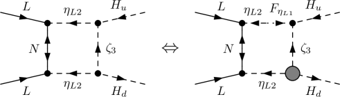
Figure 5: Leading order $A$-term (grey blobs) contribution to $LLHH$ in the model of [37]. We do not display $LLH_{u}H_{u}$ since it is subleading as it requires a $B_{\eta_{L}}$ insertion.

A thorough evaluation of soft-${{\cancel{\text{SUSY}}}_{\text{EWS}}}$ contributions to $LLHH$ up to order $2$ and in the simplifying limit $M_{N_{i}}=\mu_{s3}=\mu_{L2}=M_{N}$ is given in Appendix D.

To end this section let us briefly mention the model of [38]. It is also a one-loop 1PI seesaw and contains a Higgs bilinear. The model’s low-energy superpotential comprises Eq. (10) and Eq. (12) of [38], in addition to MSSM Yukawa couplings. In addition to baryon number, this superpotential has a continuous Abelian symmetry independent of the hypercharge and which is defined by

$$\begin{aligned} &\hat{L}\to e^{i\phi_{L}}\hat{L}\,,~{}~{}~{}~{}~{}~{}\hat{E}^{c}\to e^{-i\phi_{L}}\hat{E}^{c}\,,~{}~{}~{}~{}~{}~{}\hat{\zeta}/\hat{\eta}\to e^{\pm i\phi_{L}}\hat{\zeta}/\hat{\eta}\,,\\ &\hat{\Phi}_{u,d}\to e^{\mp i\phi_{L}}\hat{\Phi}_{u,d}\,,~{}~{}~{}~{}~{}~{}\hat{\Omega}^{\pm}\to e^{\mp i\phi_{L}}\hat{\Omega}^{\pm}\,,\end{aligned}$$ (28)

i.e. a $L$-number symmetry. The soft-${\cancel{\text{SUSY}}}$ potential of their model (cf. Eq. (11) of [38]) contains the terms

$$m^{2}_{\zeta\eta}\eta^{\dagger}\zeta+\frac{B^{2}_{\zeta}}{2}\zeta^{2}+\frac{B^{2}_{\eta}}{2}\eta^{2}+\text{H.c.}\subset-\mathcal{L}_{\text{soft}}\,,$$ (29)

which explicitly break the $U(1)_{L}$. (It is noteworthy that these terms are absent from their earlier works [40].) It is thus not surprising that in their model all $LLHH$ operators come from ${{\cancel{\text{SUSY}}}_{\text{EWS}}}$. If one adds to the superpotential the analogue of $\zeta^{2}$ and $\eta^{2}$ ${\cancel{\text{SUSY}}}$-terms, i.e.

$$\frac{M_{\zeta}}{2}\hat{\zeta}^{2}+\frac{M_{\eta}}{2}\hat{\eta}^{2}\,,$$ (30)

so that $U(1)_{L}$ breaking becomes independent of ${\cancel{\text{SUSY}}}$, one finds a pure-${{\cancel{\text{SUSY}}}_{\text{EWSB}}}$ contribution to $LLH_{u}H^{\dagger}_{d}$ and $LLH_{u}H_{u}$ in striking resemblance to the previous model: $\hat{\Phi}_{u,d}$ play the role of $\hat{\eta}_{L2,L1}$, while $\hat{\zeta}$ (and its the mixture with $\hat{\eta}$) plays the role of $\hat{\zeta}_{3}$ in the generation of $LLH_{u}H^{\dagger}_{d}$ (and $LLH_{u}H_{u}$, respectively).

3 ${{\cancel{\text{SUSY}}}_{\text{EWS}}}$ contributions

In the presence of $F$- or $D$-term ${\cancel{\text{SUSY}}}$, any operator that comes from ${{\cancel{\text{SUSY}}}_{\text{EWS}}}$ is contained in the union of the following cases:

$$\begin{aligned} &\text{a)}~{}\int d^{4}\theta\,\hat{X}\,\widehat{\text{OP}}\,;\\ &\text{b)}~{}\int d^{4}\theta\,\hat{X}^{\dagger}\,\widehat{\text{OP}}\,;\\ &\text{c)}~{}\int d^{4}\theta\,\hat{Y}\,\widehat{\text{OP}}\,;\end{aligned}$$ (31)

modulo $D^{2}\hat{X}$, $\bar{D}^{2}\hat{X}^{\dagger}$ and $D^{2}\bar{D}^{2}\hat{Y}$ insertions, and where $\hat{X}$ and $\hat{Y}$ are $F$- and $D$-term ${\cancel{\text{SUSY}}}$ spurions, respectively. Under the common assumption that ${\cancel{\text{SUSY}}}$ is blind to the internal symmetries of the visible sector, it is conceivable the existence of models in which both $\{\hat{X},\hat{X}^{\dagger},\hat{Y}\}\widehat{\text{OP}}$ (cases a, b and c, respectively) and $\widehat{\text{OP}}$ are generated up to some order in perturbation theory. We can now ask ourselves which instances of $\widehat{\text{OP}}\in\widehat{\text{OP}}_{\nu}$ do not yield an $\text{OP}\in\text{OP}_{\nu}$ in the absence of ${\cancel{\text{SUSY}}}$ spurions. The general answer is:

$$\begin{aligned} &\text{1.}~{}\widehat{\text{OP}}=D^{2}(\hat{L}\hat{L}\hat{H}^{n})\otimes\Big{(}\text{a superoperator whose $D$-term is zero at $p_{\text{ext}}=0$}\Big{)}\,;\\ &\text{2.}~{}\widehat{\text{OP}}=\hat{L}\hat{L}\otimes\Big{(}\text{a superoperator whose $F^{\dagger}$-term is zero at $p_{\text{ext}}=0$}\Big{)}\,.\end{aligned}$$ (32)

In the following, let $\hat{Z}^{\dagger}$ and $\hat{V}$ denote any superfields whose $\hat{Z}^{\dagger}~{}\text{(mod $\hat{H}^{\dagger}$)}$ and $\hat{V}~{}\text{(mod $\hat{H},\hat{H}^{\dagger}$)}$ parts satisfy Eq. (12) and Eq. (11), respectively. Type-1 superoperators that only give $\text{OP}\in\text{OP}_{\nu}$ from ${{\cancel{\text{SUSY}}}_{\text{EWS}}}$ according to a, b and c, are:

$$\begin{aligned} &\text{1.a)}~{}D^{2}(\hat{L}\hat{L}\hat{H}^{n})\otimes\left\{\hat{Z}^{\dagger},D^{2}\hat{V}\right\}\otimes\left\{\hat{H}^{\dagger},\bar{D}^{2}\hat{Z}^{\dagger},D^{2}\hat{Z},D^{2}\bar{D}^{2}\hat{V}\right\}^{n^{\prime}}\,;\\ &\text{1.b)}~{}D^{2}(\hat{L}\hat{L}\hat{H}^{n})\otimes\left\{\hat{Z},\bar{D}^{2}\hat{V}\right\}\otimes\left\{\hat{H},\bar{D}^{2}\hat{Z}^{\dagger},D^{2}\hat{Z},D^{2}\bar{D}^{2}\hat{V}\right\}^{n^{\prime}}\,;\\ &\text{1.c)}~{}D^{2}(\hat{L}\hat{L}\hat{H}^{n})\otimes\left\{(\hat{H}^{\dagger})^{k},(\hat{H})^{k}\right\}\otimes\left\{\bar{D}^{2}\hat{Z}^{\dagger},D^{2}\hat{Z},D^{2}\bar{D}^{2}\hat{V}\right\}^{n^{\prime}}\,;\end{aligned}$$ (33)

where $n,n^{\prime},k=0,1,...$ stand for any number of insertions, though constrained by internal symmetries. Type-2 $\widehat{\text{OP}}$’s that only give $\text{OP}\in\text{OP}_{\nu}$ from ${{\cancel{\text{SUSY}}}_{\text{EWS}}}$ can only proceed from b:

$$\begin{aligned} &\text{2.b)}~{}\hat{L}\hat{L}\otimes\left\{\hat{H},D^{2}\hat{Z},\bar{D}^{2}\hat{Z}^{\dagger},D^{2}\bar{D}^{2}\hat{V}\right\}^{n}\,.\end{aligned}$$ (34)

If at low energy the only Higgses are MSSM’s, then the superoperators of lowest dimension that only give $\text{OP}\in\text{OP}_{\nu}$ from ${{\cancel{\text{SUSY}}}_{\text{EWS}}}$ are

$$\begin{aligned} &\text{1.a)}~{}D^{2}(\hat{L}\hat{L})\hat{H}^{\dagger}_{d}\otimes\left\{\hat{H}^{\dagger}_{d},\bar{D}^{2}\hat{H}^{\dagger}_{d},D^{2}\hat{H}_{u}\right\}\cup D^{2}(\hat{L}\hat{L}\hat{H}_{u})\hat{H}^{\dagger}_{d}\,;\\ &\text{1.b)}~{}D^{2}(\hat{L}\hat{L})\hat{H}_{u}\otimes\left\{\hat{H}_{u},\bar{D}^{2}\hat{H}^{\dagger}_{d},D^{2}\hat{H}_{u}\right\}\cup D^{2}(\hat{L}\hat{L}\hat{H}_{u})\hat{H}_{u}\,;\\ &\text{1.c)}~{}D^{2}(\hat{L}\hat{L})\otimes\begin{aligned} \Big{\{}&D^{2}\hat{H}_{u}\otimes\left\{D^{2}\hat{H}_{u},\bar{D}^{2}\hat{H}^{\dagger}_{d}\right\},\bar{D}^{2}\hat{H}^{\dagger}_{d}\bar{D}^{2}\hat{H}^{\dagger}_{d},\\ &D^{2}(\hat{H}_{u}\hat{H}_{u}),\bar{D}^{2}(\hat{H}^{\dagger}_{d}\hat{H}^{\dagger}_{d})\Big{\}}\cup D^{2}(\hat{L}\hat{L}\hat{H}_{u}\hat{H}_{u})\cup\text{1.a}\cup\text{1.b}\,;\end{aligned}\\ &\text{2.b)}~{}\hat{L}\hat{L}\otimes\begin{aligned} \Big{\{}&\hat{H}_{u}\otimes\left\{\hat{H}_{u},D^{2}\hat{H}_{u},\bar{D}^{2}\hat{H}^{\dagger}_{d}\right\},D^{2}\hat{H}_{u}\otimes\left\{D^{2}\hat{H}_{u},\bar{D}^{2}\hat{H}^{\dagger}_{d}\right\},\\ &\bar{D}^{2}\hat{H}^{\dagger}_{d}\bar{D}^{2}\hat{H}^{\dagger}_{d},D^{2}(\hat{H}_{u}\hat{H}_{u}),\bar{D}^{2}(\hat{H}^{\dagger}_{d}\hat{H}^{\dagger}_{d})\Big{\}}\,.\end{aligned}\end{aligned}$$ (35)

3.1 Are there models in which the pure-${{\cancel{\text{SUSY}}}_{\text{EWSB}}}$ subset of $\text{OP}_{\nu}$ is empty?

Since every $\widehat{\text{OP}}\in\widehat{\text{OP}}_{\nu}$ has $U(1)_{Y}$ and $SU(2)_{L}$ charges flowing in internal lines, one might be tempted to think that this alone suffices to show that the subset is always non-empty. Indeed, as insertions of external $\hat{V}_{U(1)_{Y}}$ and $\hat{V}^{\alpha}_{SU(2)_{L}}$ into internal lines are allowed, and in particular into loop lines, it is conceivable that any $\widehat{\text{OP}}\in\widehat{\text{OP}}_{\nu}$ can be promoted to a superoperator that yields a pure-${{\cancel{\text{SUSY}}}_{\text{EWSB}}}$ $\text{OP}\in\text{OP}_{\nu}$ by means of judicious appendages of gauge vector superfields $\hat{V}$ and their chiral projections $D^{2}\hat{V}$ and $\bar{D}^{2}\hat{V}$. An example of this that we will encounter in Sec. 5 is

$$D^{2}(\hat{L}\hat{L})\hat{H}_{u}\hat{H}_{u}\to D^{2}(\hat{L}\hat{L})\hat{H}_{u}\hat{H}_{u}\hat{V}\,,$$ (36)

which yields dimension-7 operators of the form

$$LLH_{u}H_{u}H^{\dagger}H\in\text{OP}_{\nu}\,.$$ (37)

However, even though supergraphs with any given number of external $\hat{V}$’s can be constructed from any underlying $\widehat{\text{OP}}\in\widehat{\text{OP}}_{\nu}$, the so obtained $\widehat{\text{OP}}\in\widehat{\text{OP}}_{\nu}$ may vanish as the supergraphs add up to zero. In fact, this happens whenever all charge carrying internal lines undergo a chirality flip that is symmetric w.r.t. the local symmetry of which $\hat{V}$ is the gauge superfield. More generally, $\hat{V}$’s insertions can be seen to correspond to terms in the $\hat{V}$-expansion of gauge completed superoperators.

Regarding models in which there exists a Higgs bilinear. Pick a $\widehat{\text{OP}}\in\widehat{\text{OP}}_{\nu}$. Each supergraph contributing to $\widehat{\text{OP}}$ belongs to one of the following two classes:

• at least one external Higgs $\hat{H}$ (or $\hat{H}^{\dagger}$) is locally connected to loop superfields, i.e. at least one external Higgs is 1PI;

• all external Higgses are connected to the loop(s) by means of 1PR propagators, i.e. all external Higgses are 1PR.

Without loss of generality, say that for a particular supergraph belonging to class-a the vertex is $\hat{H}\hat{X}_{1}\hat{X}_{2}$, where $\hat{X}$’s are loop superfields. One can then see (cf. Fig. 6) that an insertion of $\hat{H}^{\dagger}$ ($\hat{H}$) followed by an insertion of $\hat{H}$ ($\hat{H}^{\dagger}$) leads to a supergraph for the superoperator

$$\hat{H}^{\dagger}\hat{H}\,\widehat{\text{OP}}\,.$$ (38)

Figure 6: A $\hat{H}\hat{X}_{1}\hat{X}_{2}$ vertex (leftmost diagram) implies a non-vanishing $\hat{H}\hat{H}^{\dagger}\hat{H}\hat{X}_{1}\hat{X}_{2}$ interaction that is local in $\theta$, i.e. “a vertex” from the D-algebra point of view (rightmost diagram).

Each class-b supergraph can also be transformed into a supergraph for $\hat{H}^{\dagger}\hat{H}\,\widehat{\text{OP}}$, as we proceed to show. Choose some 1PR leg. To be completely general, we take the Higgses along that leg to be $\hat{H}$, $\hat{H}^{\prime}$, …, where $\hat{H}$ is attached to the loop(s) by one 1PR propagator, $\hat{H}^{\prime}$ by two, and so on along the leg, and the chiralities are left unspecified (for e.g. $\hat{H}$ and $\hat{H}^{\prime}$ need not have the same chirality, and $\hat{H}$ can be either chiral or anti-chiral). This is depicted in the left-hand side supergraph of Fig. 7. Let $\hat{H}\hat{\Phi}\hat{\Phi}^{\prime}$ be the vertex that connects $\hat{H}$ to the leg, and where $\hat{\Phi}$ is the superfield that connects $\hat{H}$ to the loop(s) (depicted by a circle) by either a $\hat{\Phi}\hat{\Phi}^{\dagger}$ or a $\hat{\Phi}\hat{\overline{\Phi}}$ propagator. Now, in the same way as a $\hat{H}^{\dagger}\hat{H}$ insertion is performed in Fig. 6, one can make an insertion of $\hat{\Phi}^{\dagger}\hat{\Phi}$ (or $\hat{\overline{\Phi}}{}^{\dagger}\hat{\overline{\Phi}}$, depending on how $\hat{\Phi}$ is connected to the loop(s)) in the the loop line to which $\hat{\Phi}^{\dagger}$ (or $\hat{\overline{\Phi}}$) is locally connected. Then, take $\hat{\Phi}^{\dagger}$ (or $\hat{\overline{\Phi}}$) to propagate via $\hat{\Phi}\hat{\Phi}^{\dagger}$ (or $\hat{\Phi}\hat{\overline{\Phi}}$) to $\hat{\Phi}^{\prime}\hat{H}$, so that the insertion leads to two additional legs: one with $\hat{\Phi}^{\prime}\hat{H}$ and the other with $\hat{\Phi}^{\prime\dagger}\hat{H}^{\dagger}$, as shown in the middle supergraph of Fig. 7. Now, by contracting $\hat{\Phi}^{\prime}$ with $\hat{\Phi}^{\prime\dagger}$ we arrive at a supergraph (see right-hand side of Fig. 7) for the superoperator $\hat{H}^{\dagger}\hat{H}\,\widehat{\text{OP}}$.

Figure 7: Schematic of a procedure to go from a class-b supergraph for $\widehat{\text{OP}}$ (leftmost diagram) to a supergraph for $\hat{H}^{\dagger}\hat{H}\,\widehat{\text{OP}}$ (rightmost diagram) by means of a double insertion in the loop line to which the 1PR leg is attached (middle diagram). The dot at which the lines of $\hat{\Phi}^{\dagger}$ and the two $\hat{\Phi}$’s meet is a vertex in the sense of Fig. 6. In order to describe all conceivable assignments of chiralities to external and internal superfields, the chiralities of $\hat{H}$, $\hat{H}^{\prime}$, $\hat{\Phi}$ and $\hat{\Phi}^{\prime}$ are left unspecified. However, $\hat{H}$, $\hat{\Phi}$ and $\hat{\Phi}^{\prime}$ have the same chirality, as is implied by the vertex. Moreover, and so that all conceivable propagators are described, we also do not specify how $\hat{\Phi}$ is connected to the loop(s) (depicted by the circle), nor how $\hat{\Phi}^{\prime}$ is connected to $\hat{H}^{\prime}$.

The procedures described above can be applied to each class-a or -b supergraph of the set contributing to $\widehat{\text{OP}}$ up to any given order of perturbation theory. Hence, if class-a or -b supergraphs for superoperator $\widehat{\text{OP}}$ do not add up to zero, the transformed ones do not add up to zero for $\hat{H}^{\dagger}\hat{H}\,\widehat{\text{OP}}$ either. Now, if there exists a Higgs bilinear, $\hat{H}^{\dagger}\hat{H}\,\widehat{\text{OP}}$ yields a pure-${{\cancel{\text{SUSY}}}_{\text{EWSB}}}$ $\text{OP}\in\text{OP}_{\nu}$ regardless of $\widehat{\text{OP}}\in\widehat{\text{OP}}_{\nu}$. We will illustrate this for a particular model in Sec. 5.

On dimensional grounds one expects that the strength of a pure-${{\cancel{\text{SUSY}}}_{\text{EWSB}}}$ $\text{OP}\in\text{OP}_{\nu}$ obtained from $\widehat{\text{OP}}$ by an insertion of $\hat{V}$ compares to the strength of a pure-${{\cancel{\text{SUSY}}}_{\text{EWSB}}}$ $\text{OP}^{\prime}\in\text{OP}_{\nu}$ obtained from the same superoperator by an insertion of $\hat{H}^{\dagger}\hat{H}$ as

$$g^{2}:\lambda^{2}\left(\frac{\mu}{M_{X}}\right)^{2~{}\text{or}~{}1}\,,$$ (39)

for class A or B superoperators, respectively, and where $\lambda$ is the coupling strength of $\hat{H}$’s to the loop(s). Moreover, if the leading supergraphs for $\widehat{\text{OP}}$ are of class-b, and the model is such that the only feasible $\hat{H}^{\dagger}\hat{H}$ insertion is by means of the procedure described in Fig. 7, then the $\propto\mu/M$ contribution comes with an additional loop suppression factor.

4 Models in which the leading order subset of $\text{OP}_{\nu}$ is proportional to ${{\cancel{\text{SUSY}}}_{\text{EWS}}}$

A possible strategy to construct models of this kind is the following. Pick a set of superoperators that cannot yield a pure-${{\cancel{\text{SUSY}}}_{\text{EWSB}}}$ $\text{OP}\in\text{OP}_{\nu}$ (cf. Eq. (33) and Eq. (34)). Choose the LO topologies at which these operators appear. Write the necessary superfields and couplings. As a final step, pick an internal symmetry group that precludes, at least up to the same order of perturbation theory, all superoperators that yield a pure-${{\cancel{\text{SUSY}}}_{\text{EWSB}}}$ $\text{OP}\in\text{OP}_{\nu}$. In particular, it is essential that the “wrong” Higgs does not communicate (at least up to the same order as the “right” Higgs) to the sector that holds $L$-number breaking. To illustrate this, consider for example the one-loop realisation of 1PI $\hat{L}\hat{L}\hat{H}_{u}\hat{H}_{u}$. $\hat{H}_{u}$ couples to, say, $\hat{X}_{1}\hat{X}_{2}$, where $\hat{X}_{1,2}$ have mass terms. Without loss of generality let the mass terms be $\hat{\overline{X}}_{i}\hat{X}_{i}$. Hence, $\hat{\overline{X}}_{1}\hat{\overline{X}}_{2}\hat{H}_{d}$ is invariant under non-$R$-symmetries in this phase. If such a term exists in the superpotential, this same model generates the supergraph topology shown in the middle panel of Fig. 3, leading to $\hat{L}\hat{L}\hat{H}_{u}\hat{H}^{\dagger}_{d}$ which yields a pure-${{\cancel{\text{SUSY}}}_{\text{EWSB}}}$ $\text{OP}\in\text{OP}_{\nu}$.

We cannot think of any serious obstruction that would compromise this procedure for constructing general models of this kind. In fact, in the next section we give a proof of existence based on a one-loop type-II seesaw, also showing that this kind of models need not be complicated.

Under the assumption of a standard set of Higgses ($\hat{H}_{u,d}$), the simplest models of this kind are those that generate, at the one-loop order, superoperators that were identified in Eq. (35). From D-algebra considerations, and relegating topologies with self-energies to Appendix C, one obtains the following list of possibilities:

• $D^{2}(\hat{L}\hat{L})\hat{H}_{u}\hat{H}_{u}$, $\hat{L}\hat{L}D^{2}(\hat{H}_{u}\hat{H}_{u})$, $D^{2}(\hat{L}\hat{L})\hat{H}^{\dagger}_{d}\hat{H}^{\dagger}_{d}$ and $\hat{L}\hat{L}\bar{D}^{2}(\hat{H}^{\dagger}_{d}\hat{H}^{\dagger}_{d})$
  – type-II without a chirality flip;

• $\hat{L}\hat{L}\hat{H}_{u}\hat{H}_{u}$ (1PR)
  – type-II with a chirality flip, type-I and -III;

• $\hat{L}\hat{L}\hat{H}_{u}\hat{H}_{u}$ (1PI).

The corresponding supergraph topologies are depicted in Fig. 8. Notice that we populate the supergraphs with $D$’s in a manner that makes the non-trivial 1PI part separable. Moreover, when doing the D-algebra, we integrate by parts the $D$’s in a way that avoids crossing over the non-trivial 1PI part. The usefulness of this procedure is in allowing to associate superoperators to whole 1PR supergraphs, even when the result of some of their 1PI parts is zero in the SUSY limit. This works by extending the $d^{4}\theta$ integration of the non-trivial 1PI part to a $d^{4}\theta$ integration that encompasses all external superfields. To illustrate what we mean, consider the second supergraph topology, and let $\hat{\Phi}\hat{\Phi}^{\dagger}$ be the 1PR propagator. If, after doing the loop’s D-algebra, we integrated by parts the $D^{2}$ that lies over the 1PR line to the right, we would obtain $\hat{L}\hat{L}D^{2}(\hat{H}^{\dagger}_{d}\hat{H}^{\dagger}_{d})=0$. However, as we integrate it to the left, we end up with $D^{2}(\hat{L}\hat{L})\hat{H}^{\dagger}_{d}\hat{H}^{\dagger}_{d}$. With this procedure the zero of the non-trivial 1PI part, i.e. $\int d^{4}\theta\,\hat{\Phi}^{\dagger}\hat{H}^{\dagger}_{d}\hat{H}^{\dagger}_{d}=0$, is transferred to $\int d^{4}\theta\,D^{2}(\hat{L}\hat{L})\hat{H}^{\dagger}_{d}\hat{H}^{\dagger}_{d}=0$.

Figure 8: One-loop supergraph topologies that are identified in the text. From left to right: $D^{2}(\hat{L}\hat{L})\hat{H}_{u}\hat{H}_{u}$ or $\hat{L}\hat{L}D^{2}(\hat{H}_{u}\hat{H}_{u})$, $D^{2}(\hat{L}\hat{L})\hat{H}^{\dagger}_{d}\hat{H}^{\dagger}_{d}$, $\hat{L}\hat{L}\bar{D}^{2}(\hat{H}^{\dagger}_{d}\hat{H}^{\dagger}_{d})$, $\hat{L}\hat{L}\hat{H}_{u}\hat{H}_{u}$ (1PR) and $\hat{L}\hat{L}\hat{H}_{u}\hat{H}_{u}$ (1PI).

The subcase $\hat{L}\hat{L}D^{2}(\hat{H}_{u}\hat{H}_{u})$ of the first topology, i.e. in which $\hat{H}_{u}\hat{H}_{u}$ is coupled to the 1PR propagator (say $\hat{\Phi}\hat{\Phi}^{\dagger}$), contains an example of the trilinear case discussed in Sec. 2.1. To be precise, its non-trivial 1PI part gives

$$\frac{1}{M}\int d^{4}\theta\hat{L}\hat{L}\hat{\Phi}^{\dagger}\supset\frac{1}{M}LLF^{\dagger}_{\Phi}\,,$$ (40)

and since (cf. Eq. (70) and let $\lambda$ be the $\hat{\Phi}\hat{H}_{u}\hat{H}_{u}$ superpotential coupling)

$$\langle F^{\dagger}_{\Phi}\rangle=\frac{m_{\text{soft}}^{2}}{M_{\Phi}^{2}}\lambda\langle H_{u}H_{u}\rangle+\frac{\lambda B^{*}}{M_{\Phi}^{3}}\left(A\langle H_{u}H_{u}\rangle+2\mu^{*}\langle H_{u}H^{\dagger}_{d}\rangle\right)+\mathcal{O}\left(\frac{m_{\text{soft}}^{4}}{M^{4}_{\Phi}}\right)\,,$$ (41)

it effectively generates $LLH_{u}H_{u}$ and $LLH_{u}H^{\dagger}_{d}$.

To study how ${\cancel{\text{SUSY}}}$ effects upon these topologies can generate an $\widehat{\text{OP}}$ which yields an $\text{OP}\in\text{OP}_{\nu}$, we include soft-${\cancel{\text{SUSY}}}$ in supergraph calculations by means of the following non-chiral vertices with ${\cancel{\text{SUSY}}}$ spurions ($\hat{X}\sim M_{X}^{2}\theta^{2}$):

$$\begin{aligned} &\lambda A\phi_{1}\phi_{2}\phi_{3}=\lambda\int d^{4}\theta\left(\frac{X^{\dagger}X}{M_{X}^{3}}\right)_{A}\hat{\Phi}_{1}\hat{\Phi}_{2}\hat{\Phi}_{3}\,,\\ &B\phi_{1}\phi_{2}=\int d^{4}\theta\left(\frac{X^{\dagger}X}{M_{X}^{2}}\right)_{B}\hat{\Phi}_{1}\hat{\Phi}_{2}\,,\\ &m_{\text{soft}}^{2}\phi_{1}^{\dagger}\phi_{1}=\int d^{4}\theta\left(\frac{X^{\dagger}X}{M_{X}^{2}}\right)_{m_{\text{soft}}^{2}}\hat{\Phi}_{1}^{\dagger}\hat{\Phi}_{1}\,.\end{aligned}$$ (42)

We note that this form for $A$- and $B$-terms is equivalent to (d) and (b) of [35], respectively, since $\int d^{4}\theta\hat{X}^{\dagger}\hat{X}\,\widehat{\text{OP}}\sim\int d^{2}\theta\hat{X}\,\widehat{\text{OP}}$ (). The complete list of ${\cancel{\text{SUSY}}}$ insertions that yield an $\text{OP}\in\text{OP}_{\nu}$ reads

$$\begin{aligned} &\int d^{4}\theta\left[D^{2}(\hat{X}^{\dagger}\hat{X})~{}\text{or}~{}\hat{X}^{\dagger}\hat{X}\right]\left\{D^{2}\bar{D}^{2}(\hat{X}^{\dagger}\hat{X})\right\}^{n}D^{2}(\hat{L}\hat{L})\hat{H}_{u}\hat{H}_{u}\,,\\ &\int d^{4}\theta\,\left\{D^{2}\bar{D}^{2}(\hat{X}^{\dagger}\hat{X})\right\}^{n}\hat{L}\hat{L}\,\Big{\{}\begin{aligned} &D^{2}(\hat{X}^{\dagger}\hat{X}\hat{H}_{u}\hat{H}_{u}),\\ &D^{2}(\hat{X}^{\dagger}\hat{X})\left[D^{2}(\hat{H}_{u}\hat{H}_{u})~{}\text{or}~{}D^{2}(\hat{H}_{u}\hat{H}_{u}\bar{D}^{2}(\hat{X}^{\dagger}\hat{X}))\right]\Big{\}}\,,\end{aligned}\\ &\int d^{4}\theta\left[\bar{D}^{2}(\hat{X}^{\dagger}\hat{X})~{}\text{or}~{}\hat{X}^{\dagger}\hat{X}\right]\left\{D^{2}\bar{D}^{2}(\hat{X}^{\dagger}\hat{X})\right\}^{n}D^{2}(\hat{L}\hat{L})\hat{H}_{d}^{\dagger}\hat{H}_{d}^{\dagger}\,,\\ &\int d^{4}\theta\,D^{2}(\hat{X}^{\dagger}\hat{X})\left\{D^{2}\bar{D}^{2}(\hat{X}^{\dagger}\hat{X})\right\}^{n}\hat{L}\hat{L}\left[\bar{D}^{2}(\hat{H}_{d}^{\dagger}\hat{H}_{d}^{\dagger})~{}\text{or}~{}\bar{D}^{2}(\hat{H}_{d}^{\dagger}\hat{H}_{d}^{\dagger}D^{2}(\hat{X}^{\dagger}\hat{X}))\right]\,,\\ &\int d^{4}\theta\,D^{2}(\hat{X}^{\dagger}\hat{X})\left\{D^{2}\bar{D}^{2}(\hat{X}^{\dagger}\hat{X})\right\}^{n}\hat{L}\hat{L}\hat{H}_{u}\hat{H}_{u}\,,\end{aligned}$$ (43)

where $n=0,1,...$ stands for the number of insertions of $D^{2}\bar{D}^{2}(\hat{X}^{\dagger}\hat{X})$.

A soft-${\cancel{\text{SUSY}}}$ insertion into a (anti-)chiral vertex, i.e. an $A$-term, introduces an extra $\hat{X}$ ($\hat{X}^{\dagger}$, respectively) factor in the corresponding supergraph. Hence, D-algebra considerations reveal that a single soft-${\cancel{\text{SUSY}}}$ insertion of an $A$-term can generate an $\text{OP}\in\text{OP}_{\nu}$ only in the case of a type-II seesaw without a chirality flip, i.e. the first topology of Fig. 8, and which leads to

$$\frac{A^{*}\mu^{*}}{M^{3}}LLH_{u}H^{\dagger}_{d}\subset\frac{1}{M^{3}}\int d^{4}\theta\,D^{2}\left(\frac{\hat{X}^{\dagger}\hat{X}}{M_{X}^{3}}\right)_{A^{*}}\left[D^{2}(\hat{L}\hat{L})\hat{H}_{u}\hat{H}_{u}~{}\text{or}~{}\hat{L}\hat{L}D^{2}(\hat{H}_{u}\hat{H}_{u})\right]\,.$$ (44)

For a detailed catalogue up to order $3$ in the scale of soft-${\cancel{\text{SUSY}}}$ ($m_{\text{soft}}$) see Appendix B. It is important to notice that ${\cancel{\text{SUSY}}}$-insertions into the supergraph underlying the superoperator $\hat{L}\hat{L}D^{2}(\hat{H}_{u}\hat{H}_{u})$ do yield the $\langle F^{\dagger}_{\Phi}\rangle$ contribution mentioned in Eq. (41). Indeed, the terms in Eq. (41) correspond respectively to the following entries of Tab. 5: the 5th row of the second table and the 4th and 1st rows of the first table.

From the tables in Appendix B three different kinds of leading dimensionful suppression factors are found:

• $\mu\,m_{\text{soft}}/M^{3}$ or $m_{\text{soft}}^{2}/M^{3}$ – $D^{2}(\hat{L}\hat{L})\hat{H}_{u}\hat{H}_{u}$ and $\hat{L}\hat{L}D^{2}(\hat{H}_{u}\hat{H}_{u})$;

• $\mu\,m_{\text{soft}}^{2}/M^{4}$ or $m_{\text{soft}}^{3}/M^{4}$ – $\hat{L}\hat{L}\bar{D}^{2}(\hat{H}^{\dagger}_{d}\hat{H}^{\dagger}_{d})$;

• $m_{\text{soft}}^{2}/M^{3}$ – $D^{2}(\hat{L}\hat{L})\hat{H}^{\dagger}_{d}\hat{H}^{\dagger}_{d}$ and $\hat{L}\hat{L}\hat{H}_{u}\hat{H}_{u}$ (both 1PR and 1PI).

The absence of a contribution linear in $m_{\text{soft}}$ for some topologies is most easily seen to stem from the fact that one-loop topologies for $\hat{L}\hat{L}\hat{H}_{u}\hat{H}_{u}$, as well as the one-loop 1PI parts of $D^{2}(\hat{L}\hat{L})\hat{H}^{\dagger}_{d}\hat{H}^{\dagger}_{d}$ and $\hat{L}\hat{L}\bar{D}^{2}(\hat{H}^{\dagger}_{d}\hat{H}^{\dagger}_{d})$, use vertices of a single chirality. Moreover, and in regard to $\hat{L}\hat{L}\bar{D}^{2}(\hat{H}^{\dagger}_{d}\hat{H}^{\dagger}_{d})$, the leading contributions from the $\bar{D}^{2}(\hat{H}^{\dagger}_{d}\hat{H}^{\dagger}_{d})$ piece are $\mu H_{u}H^{\dagger}_{d}$ and $A^{*}H^{\dagger}_{d}H^{\dagger}_{d}$.

In Appendix C, where we conduct a similar analysis for one-loop realisations with self-energies, we find that these too have leading dimensionful suppression factors that range from $\mu\,m_{\text{soft}}/M^{3}$ or $m_{\text{soft}}^{2}/M^{3}$ to $\mu\,m_{\text{soft}}^{2}/M^{4}$ or $m_{\text{soft}}^{3}/M^{4}$.

If we take $\mu\sim m_{\text{soft}}$, we can conclude that in one-loop models of this kind $LLHH$ operators have a dimensionful suppression of at least $m_{\text{soft}}^{2}/M^{3}$. This result is naively expected for type-II seesaws without a chirality flip, since $\int d^{4}\theta D^{2}(\hat{L}\hat{L})\hat{H}\hat{H}$ has mass dimension $7$. For other realisations this dependence is not trivial, since for an underlying superoperator $\hat{L}\hat{L}\hat{H}\hat{H}$ one in general expects a $m_{\text{soft}}/M^{2}$ dependence, as was indeed found in Sec. 2.2.

The dimensionful suppression $\mu\,m_{\text{soft}}/M^{3}$ or $m_{\text{soft}}^{2}/M^{3}$ does not hold at higher loops. For instance, consider $\hat{L}\hat{L}\hat{H}_{u}\hat{H}_{u}$ generated by the 1PI two-loop topology shown in the left-hand side of Fig. 9. A single $A$-term insertion (depicted as a grey blob, on the right) leads to

$$\frac{1}{M^{2}}\int d^{4}\theta\,D^{2}\left(\frac{\hat{X}^{\dagger}\hat{X}}{M_{X}^{3}}\right)_{A^{*}}\hat{L}\hat{L}\hat{H}_{u}\hat{H}_{u}\supset\frac{A^{*}}{M^{2}}LLH_{u}H_{u}\,.$$ (45)

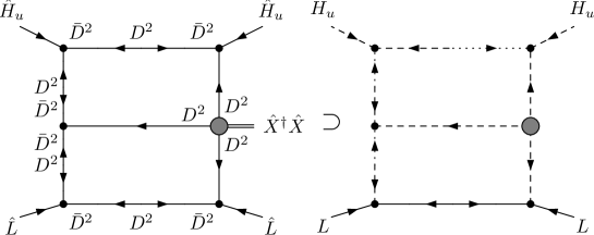
Figure 9: Example of a two-loop supergraph for superoperator $\hat{L}\hat{L}\hat{H}_{u}\hat{H}_{u}$ (left) which yields an $\text{OP}\in\text{OP}_{\nu}$ by means of a single $A$-term insertion (right).

5 A model example

Looking at the one-loop topology for $D^{2}(\hat{L}\hat{L})\hat{H}_{u}\hat{H}_{u}$ (cf. Fig. 8) we see that the most general set of scalar superfields and superpotential terms involved is $7$ and $5$ ($4$ trilinears and $1$ bilinear), respectively. The subset of $U(1)^{7}$ (acting independently on each scalar superfield) under which the $5$ terms are invariant consists of the hypercharge and a new $U(1)_{X}$ charge carried by the superfields in the loop (say $\hat{X}$’s). These are responsible for communicating $L$-number breaking to the SM leptons via the exchange of a type-II seesaw mediator, $\hat{\Delta}$.

Since $\hat{\Delta}$ must be massive, the only way by which the coupling $\hat{\Delta}^{\dagger}\hat{H}_{u}\hat{H}_{u}$ can be made to be genuinely radiative is by linking it to the VEV of a superoperator of at least dimension $4$ in superfields. One simple example is

$$\hat{\rho}^{\dagger}\hat{\Delta}^{\dagger}\hat{H}_{u}\hat{H}_{u}\to\langle\rho^{\dagger}\rangle\hat{\Delta}^{\dagger}\hat{H}_{u}\hat{H}_{u}+\hat{\rho}^{\dagger}\hat{\Delta}^{\dagger}\hat{H}_{u}\hat{H}_{u}\,.$$ (46)

This is similar to the procedure described in [18] to prevent a 1PR seesaw from having a tree-level contribution and which in an ordinary QFT only works for type-I and -III topologies. It can be successfully applied to the type-II topology in a SUSY setting because renormalisable four-scalar interactions can be genuinely radiative in SUSY (see Appendix E). To understand this result, we note the following. In order for the $\chi\chi\phi$ interaction to be genuinely radiative, and thus realise a radiative type-I or -III seesaw, it must arise from some symmetric operator that is not present at tree-level in the UV complete model. Only non-renormalisable operators satisfy this criterion. Thus, if one builds a model in which $\chi\chi\phi\phi^{\prime}$ is not generated at tree-level (this can always be done) and $\phi^{\prime}$ gets a symmetry breaking VEV, in the broken phase we obtain the so desired radiative coupling. (The way by which this is done in [18] is to consider that $\phi^{\prime}$ is attached to an internal spinor line of an underlying 1PI one-loop topology for $\chi\chi\phi\phi^{\prime}$.) In an ordinary QFT this cannot work for a target $\phi^{3}$ from a symmetric $\phi^{3}\phi^{\prime}$ because $\phi^{3}\phi^{\prime}$, being renormalisable, must be present at tree-level in the UV complete model.

We will assume that this is achieved by a $U(1)$ $L$-number symmetry that is broken by the VEV of the scalar component of $\hat{\rho}$. Since $L$-number breaking is communicated by $X$’s, the simplest choice is to consider that they couple directly to $\hat{\rho}$. We remain agnostic as to what drives $\langle\rho\rangle\neq 0$. Furthermore, the simplest holomorphy compliant choice is to make a $\hat{\rho}^{\dagger}$ insertion in the loop line where chirality flips, so that the mass term originates from $L$-number breaking. We thus arrive at the left-hand side diagram of Fig. 10. Even though the topology does not require $\hat{X}_{1}$ and $\hat{X}_{2}$ to have mass terms, we will assume that they do have $\hat{X}\hat{\overline{X}}$ mass terms already at the $L$-number symmetric phase.

Figure 10: Leading order subset of $\widehat{\text{OP}}_{\nu}$ in the model example.

The model is thus summarised in Tab. 1 and its most general renormalisable superpotential reads

$$\mathcal{W} := \mathcal{W}_{\text{MSSM}}+M_{\Delta}\hat{\Delta}\hat{\overline{\Delta}}+\sum_{i=1}^{2}M_{X_{i}}\hat{X}_{i}\hat{\overline{X}}_{i}+\lambda\hat{\rho}\hat{X}_{3}\hat{\overline{X}}_{3}$$ (47)

$$+\hat{H}_{u}\left(\lambda_{1}\hat{X}_{1}\hat{\overline{X}}_{3}+\lambda_{2}\hat{X}_{2}\hat{X}_{3}\right)+\hat{\Delta}\left(\lambda_{L}\hat{L}\hat{L}+\lambda_{X}\hat{X}_{1}\hat{X}_{2}\right)+\bar{\lambda}_{X}\hat{\overline{\Delta}}\,\hat{\overline{X}}_{1}\hat{\overline{X}}_{2}\,.$$

(Conventions regarding $SU(2)_{L}$ contractions are given in Appendix F.) In the absence of the last term the model acquires the $R$-symmetry shown in the last column of Tab. 1. This term allows for a chirality flipped type-II seesaw of superoperator $\hat{L}\hat{L}\hat{H}_{u}\hat{H}_{u}$, as shown in the right-hand side supergraph of Fig. 10. The broken $L$-number phase corresponds to

$$\lambda\hat{\rho}\hat{X}_{3}\hat{\overline{X}}_{3}\to M_{X_{3}}\hat{X}_{3}\hat{\overline{X}}_{3}+\lambda\hat{\rho}\hat{X}_{3}\hat{\overline{X}}_{3}\,,~{}~{}~{}M_{X_{3}}:=\lambda\langle\rho\rangle\,.$$ (48)

	$SU(2)_{L}\otimes U(1)_{Y}$	$U(1)_{X}$	$U(1)_{L}$	$U(1)_{R}$
$\hat{\Delta}$	$(\mathbf{3},1)$	$0$	$-2$	$4$
$\hat{\rho}$	$(\mathbf{1},0)$	$0$	$2$	$0$
$\hat{X}_{1}$	$(\mathbf{2},-1/2)$	$1$	$1$	$-2$
$\hat{X}_{2}$	$(\mathbf{2},-1/2)$	$-1$	$1$	$0$
$\hat{X}_{3}$	$(\mathbf{1},0)$	$1$	$-1$	$0$
$\hat{\overline{X}}_{3}$	$(\mathbf{1},0)$	$-1$	$-1$	$2$

Table 1: Extension of the MSSM in the model example. We omitted the conjugates of $\hat{\Delta}$ and $\hat{X}_{1,2}$. $U(1)_{R}$ stands for an $R$-symmetry that is acquired as $\bar{\lambda}_{X}\to 0$.

It is now convenient to notice that, as any coupling in $\{\lambda_{1},\lambda_{2},\lambda_{L}\}$, or both $\lambda_{X}$ and any in $\{\bar{\lambda}_{X},M_{\Delta},M_{X_{1}},M_{X_{2}}\}$, goes to zero the model recovers a $L$-number symmetry, any superoperator that breaks $L$-number must be proportional to

$$\mathbf{a}:=\lambda_{1}\lambda_{2}\boldsymbol{\lambda_{L}}\lambda_{X}^{*}~{}~{}\text{or}~{}~{}M_{\Delta}M_{X_{1}}M_{X_{2}}\,\mathbf{b}:=\lambda_{1}\lambda_{2}\boldsymbol{\lambda_{L}}\bar{\lambda}_{X}M_{\Delta}M_{X_{1}}M_{X_{2}}\,.$$ (49)

Hence, the set of LO (w.r.t. perturbation theory only, i.e. disregarding hypothetical hierarchies among couplings or masses) superoperators that break $L$-number proceed from the two supergraphs of Fig. 10 (and no others) and are

$$D^{2}(\hat{L}\hat{L})\hat{H}_{u}\hat{H}_{u}\,,~{}~{}~{}\hat{L}\hat{L}\hat{H}_{u}\hat{H}_{u}\,.$$ (50)

In the $p_{\text{ext}}\to 0$ limit the LO coefficients are given by

$$-\left(\frac{\mathbf{a}M_{X_{3}}}{32\pi^{2}M_{\Delta}^{2}}\right)C_{0}\,,~{}~{}~{}~{}\left(\frac{\mathbf{b}M_{X_{3}}M_{X_{1}}M_{X_{2}}}{32\pi^{2}M_{\Delta}}\right)D_{0,0}\,,$$ (51)

respectively, and where $C_{0}$ and $D_{0}$ are abbreviations of scalar one-loop 3- and 4-point integrals, respectively, as defined in Appendix F. In the SUSY limit LO $L$-number breaking is thus

$$\int d^{4}\theta\,D^{2}(\hat{L}\hat{L})\hat{H}_{u}\hat{H}_{u} = -\Box(\tilde{L}\tilde{L})\left[\tilde{H}_{u}\tilde{H}_{u}+2F_{H_{u}}H_{u}\right]-\Box(H_{u}H_{u})\left[LL+2F_{L}\tilde{L}\right]$$ (52)

$$+4\,(p_{L}+p_{\tilde{L}})^{2}\,L\tilde{H}_{u}\tilde{L}H_{u}\,,$$

while $\int d^{4}\theta\hat{L}\hat{L}\hat{H}_{u}\hat{H}_{u}=0$. Hence, we see that there is no pure-${{\cancel{\text{SUSY}}}_{\text{EWSB}}}$ contribution to neutrino masses. An equivalent way to arrive at this conclusion is the following. Of the two supergraphs, only the first has a non-vanishing (non-trivial) 1PI part. It reads

$$\int d^{4}\theta\,\hat{\Delta}^{\dagger}\hat{H}_{u}\hat{H}_{u}=2\tilde{\Delta}^{\dagger\dot{\alpha}}(p_{\tilde{H}_{u}}+p_{H_{u}})_{\beta\dot{\alpha}}{\tilde{H}}_{u}^{\beta}H_{u}+F^{\dagger}_{\Delta}\left(\tilde{H}_{u}\tilde{H}_{u}+2F_{H_{u}}H_{u}\right)-\Delta^{\dagger}\Box(H_{u}H_{u})\,.$$ (53)

Then, by adding to the classical Lagrangian these operators, one sees that $\langle F_{H_{u}}\rangle=\mu^{*}\langle H^{\dagger}_{d}\rangle\neq 0$ generates a tadpole contribution to $F^{\dagger}_{\Delta}\supset M_{\Delta}{\overline{\Delta}}$. Thus, ${\overline{\Delta}}$ acquires a VEV. However, as there is no mixing between ${\overline{\Delta}}$ and $\Delta$, this VEV is inconsequential for neutrino masses. On the other hand, when ${{\cancel{\text{SUSY}}}_{\text{EWS}}}$ contributions are considered, $\langle{\overline{\Delta}}\rangle\neq 0$ will give a contribution to neutrino masses by means of the soft-${\cancel{\text{SUSY}}}$ term $B_{\Delta}\Delta{\overline{\Delta}}$. We will comment on this below.

It is instructive to illustrate in terms of component fields why there is no pure-${{\cancel{\text{SUSY}}}_{\text{EWSB}}}$ contribution to $LLHH$. In order to yield $LLHH$, the first supergraph of Fig. 10 necessitates the three-scalar coupling $\Delta^{\dagger}H_{u}H_{u}$. There are three topologies contributing to this coupling at LO: two with scalars in the loop and the other with spinors (see Fig. 11). In the $p_{\text{ext}}\to 0$ limit the latter cancels the former exactly. Another way to look at this result is the following. If one draws diagrams for $\Delta^{\dagger}H_{u}H_{u}$ using auxiliary fields – so that holomorphy becomes more transparent – one concludes that there does not exist a single diagram that is simultaneously holomorphy compliant and has at least an external $F^{\dagger}-F$ pair. Moreover, all such diagrams that are holomorphy compliant can be paired in sets in such a way that a set with scalar loops is matched to a set with spinor loops and an exact cancellation in the $p_{\text{ext}}\to 0$ limit is operative. Regarding the second supergraph, it necessitates $F_{\overline{\Delta}}H_{u}H_{u}$ but no holomorphy compliant diagram for $F_{\overline{\Delta}}H_{u}H_{u}$ can be drawn.

Figure 11: Leading order diagrams for $\Delta^{\dagger}H_{u}H_{u}$ in the model example.

By recalling the discussion in Sec. 3.1, one can see that the pure-${{\cancel{\text{SUSY}}}_{\text{EWSB}}}$ subset of $\text{OP}_{\nu}$ comprises at LO the dimension-7 operators generated by the supergraphs depicted in Fig. 12. (Insertions of gauge vector superfields into the second supergraph of Fig. 10 have been omitted as they add up to zero, cf. Sec. 3.1.) They generate the superoperators

$$D^{2}(\hat{L}\hat{L})\hat{H}_{u}\hat{H}_{u}\hat{V}_{U(1)_{Y}}\,,~{}~{}D^{2}(\hat{L}\hat{L})\hat{H}_{u}\hat{H}_{u}\hat{V}_{SU(2)_{L}}\,,~{}~{}D^{2}(\hat{L}\hat{L})\hat{H}_{u}\hat{H}_{u}\hat{H}^{\dagger}_{u}\hat{H}_{u}\,,~{}~{}\hat{L}\hat{L}\hat{H}_{u}\hat{H}_{u}\hat{H}_{u}^{\dagger}\hat{H}_{u}\,,$$ (54)

with LO coefficients

$$\begin{aligned} &\frac{g^{\prime}\mathbf{a}M_{X_{3}}C_{0}}{32\pi^{2}M_{\Delta}^{2}}\,,~{}~{}~{}~{}\frac{g\mathbf{a}M_{X_{3}}C_{0}}{16\pi^{2}M_{\Delta}^{2}}\,,\\ &-\frac{\mathbf{a}M_{X_{3}}}{32\pi^{2}M_{\Delta}^{2}}\sum_{i=1}^{2}|\lambda_{i}|^{2}\left(D_{0,3}+M_{X_{i}}^{2}E_{0,i}\right)\,,~{}~{}~{}~{}\frac{\mathbf{b}M_{X_{3}}M_{X_{1}}M_{X_{2}}}{32\pi^{2}M_{\Delta}}\sum_{i=1}^{2}|\lambda_{i}|^{2}E_{0,i}\,,\end{aligned}$$ (55)

respectively. More explicit expressions are given in Appendix F.1, in particular Eq. (89) and Eq. (91). Hence, the LO pure-${{\cancel{\text{SUSY}}}_{\text{EWSB}}}$ subset of $\text{OP}_{\nu}$ is

$$-\frac{1}{64\pi^{2}M_{\Delta}^{2}M_{X}}\Bigg{(} \mathbf{a}\Bigg{[}\begin{aligned} &\frac{g^{2}}{2c_{w}^{2}}\left(LH_{u}\right)\left(LH_{u}\right)H^{\dagger}_{u}H_{u}+\left(\frac{g^{2}c_{2w}}{2c_{w}^{2}}+\frac{|\mu|^{2}(|\lambda_{1}|^{2}+|\lambda_{2}|^{2})}{6M_{X}^{2}}\right)\left(LH_{u}\right)\left(LH_{u}\right)H^{\dagger}_{d}H_{d}\\ &+\left(g^{2}-\frac{|\mu|^{2}(|\lambda_{1}|^{2}+|\lambda_{2}|^{2})}{3M_{X}^{2}}\right)\left(LH_{u}\right)\left(H_{u}H_{d}\right)H^{\dagger}_{d}L\Bigg{]}\end{aligned}$$

$$+\frac{\mathbf{b}M_{\Delta}\mu\,(|\lambda_{1}|^{2}+|\lambda_{2}|^{2})}{6M_{X}^{2}}\left(LH_{u}\right)\left(LH_{u}\right)\left(H_{u}H_{d}\right)\Bigg{)}\,,$$ (56)

where we have taken the simplifying limit $M_{X_{1,2,3}}=M_{X}$ (cf. Eq. (90) and Eq. (92)). From this expression we can see that the gauge couplings’ contribution to neutrino masses, which reads

$$\mathbf{m^{{\cancel{\text{SUSY}}}_{\text{EWSB}}}_{\nu}}\supset-\frac{g^{2}\mathbf{a}}{64\pi^{2}c_{w}^{2}}\frac{v^{4}}{M_{\Delta}^{2}M_{X}}c_{2\beta}s_{\beta}^{2}\,,$$ (57)

vanishes at $v_{u}=v_{d}$. This agrees with the fact that the contribution is $\propto\langle D\rangle$ since $v_{u}=v_{d}$ corresponds to the $D$-flat direction of the scalar potential.

Figure 12: Leading order supergraphs for the pure-${{\cancel{\text{SUSY}}}_{\text{EWSB}}}$ subset of $\text{OP}_{\nu}$ in the model example.

To understand, in terms of component fields, how these insertions are enablers of contributions to $\text{OP}_{\nu}$ consider the following. As the insertion of an external auxiliary component of a gauge vector superfield ($D$) into a scalar line preserves chirality (or, diagrammatically, the arrowhead’s direction), any holomorphy compliant diagram with a $D$ attached has a corresponding (underlying) holomorphy compliant diagram without that $D$. Since in our example we are considering a single $D$ insertion, the LO underlying diagrams are the ones depicted in Fig. 11, and no others. Once an external $D$ is attached to an internal scalar line, the spinor loop diagram does not contribute and the sum of the others need not vanish anymore to respect the SUSY non-renormalisation theorem. Regarding the $\hat{H}^{\dagger}_{u}\hat{H}_{u}$ insertion, one can see that it allows for holomorphy compliant diagrams with an external $F^{\dagger}-F$ pair by means of attaching $F^{\dagger}_{H_{u}}$ and $F_{H_{u}}$ to the scalar loop.

The LO subset of $\text{OP}_{\nu}$ is composed of dimension-5 operators that come from ${{\cancel{\text{SUSY}}}_{\text{EWS}}}$. Complete expressions for these operators up to order $3$ in $m_{\text{soft}}$ are given in Appendix F.2. Here we take the simplifying limits $M_{X_{1,2,3}}=M_{X}$, $(m_{\text{soft}}^{2})_{X_{1,2,3}}=(m_{\text{soft}}^{2})_{\overline{X}_{1,2,3}}=m_{\text{soft}}^{2}$, $A_{1,2}=A$ and $B_{X_{1,2,3}}=B_{X}$. Eq. (93) then reads

$$\frac{1}{64\pi^{2}M_{\Delta}^{2}}\left(\mathbf{a}\left[\frac{2m_{\text{soft}}^{2}}{M_{X}}+\frac{2A}{M_{X}}\left(A^{*}_{X}-\frac{B_{\Delta}}{M_{\Delta}}\right)-\frac{A^{*}_{X}B_{X}}{M_{X}^{2}}\right]+\mathbf{b}M_{\Delta}\frac{B_{X}}{M_{X}^{2}}\right)LLH_{u}H_{u}$$

$$-\frac{\mathbf{a}}{32\pi^{2}M_{\Delta}^{2}}\left(\frac{\mu^{*}}{M_{X}}\right)\left[A^{*}_{X}\left(1-\frac{m_{\text{soft}}^{2}}{M_{X}^{2}}-\frac{(m_{\text{soft}}^{2})_{\Delta}}{M_{\Delta}^{2}}\right)-\frac{B_{\Delta}}{M_{\Delta}}\right]LLH_{u}H^{\dagger}_{d}$$

$$-\frac{\mathbf{a}}{192\pi^{2}M_{\Delta}^{2}}\left(\frac{\mu^{*}}{M_{X}}\right)^{2}\frac{A^{*}_{X}B_{X}}{M_{X}^{2}}LLH_{d}^{\dagger}H^{\dagger}_{d}\,.$$ (58)

The discussion surrounding Fig. 11 already suggested that one type of ${\cancel{\text{SUSY}}}$ contribution would come from the mass splittings within components of chiral scalar superfields, as induced by $m_{\text{soft}}^{2}$ and $B_{X}$, since they introduce a mismatch in the cancellation between spinor and scalar loops. However, unlike $m_{\text{soft}}^{2}$, $B$ insertions reverse chirality. Thus, while a single chirality flip in a scalar line makes holomorphy compliant diagrams for $F_{\overline{\Delta}}H_{u}H_{u}$ possible – and that is why there is a $B_{X}$-term contribution from the second supergraph (identified by the $\mathbf{b}$ dependence in the expression above) –, a single ${\cancel{\text{SUSY}}}$ insertion of a $B_{X}$ disables holomorphy compliant diagrams for $\Delta^{\dagger}H_{u}H_{u}$ and hence the absence of a single $B_{X}$-term contribution proportional to $\mathbf{a}$ for $LLH_{u}H_{u}$ (cf. Eq. (93)). For $LLH_{u}H^{\dagger}_{d}$ such a contribution can be holomorphy compliant due to an external $F$ ($F_{H_{u}}\to\mu^{*}H^{\dagger}_{d}$). Concerning contributions proportional to $B_{\Delta}$, they rely on the fact that EWSB induces, at the one-loop level, a VEV for ${\overline{\Delta}}$ which, through $B_{\Delta}$, induces a VEV for $\Delta$ and hence $LL\langle\Delta\rangle\subset\int d^{2}\theta\,\mathcal{W}$. In fact, one can confirm that the dependence of $LLH_{u}H^{\dagger}_{d}$ on $B_{\Delta}$ is what one obtains from $LL\langle\Delta\rangle$, where $\langle\Delta\rangle$ is computed by following the route

$$\langle H\rangle\xrightarrow[\int d^{4}\theta\,\hat{\Delta}^{\dagger}\hat{H}_{u}\hat{H}_{u}]{}\langle{\overline{\Delta}}\rangle\xrightarrow[B_{\Delta}\Delta{\overline{\Delta}}]{}\langle\Delta\rangle\,.$$ (59)

In order to obtain the $B_{\Delta}$ dependence of $LLH_{u}H_{u}$, one must take into account the shift in $\langle{\overline{\Delta}}\rangle$ induced by ${\cancel{\text{SUSY}}}$. To leading order, this shift is proportional to $A_{1}+A_{2}$.

6 Conclusions

While the smallness of $m_{\nu}$ points towards an high seesaw scale $M$, the resolution of the hierarchy problem suggests that the scale of soft-${\cancel{\text{SUSY}}}$ should lie close to the TeV scale. It is then tempting to conceive that $m_{\text{soft}}/M$ is partially responsible for $m_{\nu}\ll v$. Since in the SUSY limit there are no radiative corrections to the superpotential, models in which neutrino masses arise at the loop level provide a scenario in which such a connection is natural. How $m_{\nu}$ is proportional to ${\cancel{\text{SUSY}}}$ depends on the particular radiative seesaw model or, more specifically, on the form of the leading $L$-number breaking superoperators.

By classifying the dependence on ${\cancel{\text{SUSY}}}$ according to their involvement in EWSB, we identified a subset of model-topologies in which the leading contributions to $m_{\nu}$ depend on ${\cancel{\text{SUSY}}}$ sources that are not involved in EWSB. In a first stage, we argued in favour of this by showing that, of all superoperators that can possibly contribute to neutrino masses, there is a subset which does it only by means of insertions of ${\cancel{\text{SUSY}}}$ spurions. Then, in a second stage, we gave a complete description of the simplest model-topologies in which all leading superoperators were of this type, and calculated their dependence on soft-${\cancel{\text{SUSY}}}$ up to order $3$. We found that all one-loop realisations generated $LLHH$ operators with a leading dimensionful dependence that ranged from $\mu\,m_{\text{soft}}/M^{3}$ or $m_{\text{soft}}^{2}/M^{3}$ to $\mu\,m_{\text{soft}}^{2}/M^{4}$ or $m_{\text{soft}}^{3}/M^{4}$.

Even though the majority of all conceivable model-topologies do in fact generate contributions to $m_{\nu}$ proportional to ${{\cancel{\text{SUSY}}}_{\text{EWS}}}$, we pointed out that all models in the literature that we are aware of generate at least one leading topology that gives a contribution in which all ${\cancel{\text{SUSY}}}$ sources are involved in EWSB. To serve as a proof of existence of models in which $m_{\nu}$ is proportional to ${{\cancel{\text{SUSY}}}_{\text{EWS}}}$ at leading order, we built a model in which the leading neutrino mass operators were of dimension-5 and came from ${{\cancel{\text{SUSY}}}_{\text{EWS}}}$, whereas the pure-${{\cancel{\text{SUSY}}}_{\text{EWSB}}}$ ones had dimension-7.

One phenomenologically interesting aspect of these models is that soft-${\cancel{\text{SUSY}}}$ effects generating the leading order $m_{\nu}$ can be quite small without conflicting with lower limits on the mass of new particles. This is due to the fact that these effects involve states that can possess superpotential mass terms in the EWS phase, as we have seen in the model example. This is in contrast with models that contain pure-${{\cancel{\text{SUSY}}}_{\text{EWSB}}}$ contributions to $m_{\nu}$ at leading order, because $\mu$ and the soft-${\cancel{\text{SUSY}}}$ effects driving EWSB provide the dominant contribution to the mass of the corresponding states, and are therefore severely constrained by present lower limits on sparticle masses.

If one conceives the leading order $m_{\nu}$ to be small as a result of some small scale (say $m$) in the underlying soft-${\cancel{\text{SUSY}}}$ effects, its explanatory value for the smallness of $m_{\nu}$ must be confronted with the size of next-to-leading order contributions that are insensitive to $m$. These next-to-leading contributions do appear at the same loop level in the form of operators of higher dimension, but can also appear as higher-loop contributions to operators of leading dimension. For instance, in the model example the former were dimension-7 operators proportional to $\mu/M$ or $g^{2}$, whereas the latter arise as two-loop contributions to dimension-5 operators. These are proportional to:

• $\mu^{2}/M^{2}$ (and $\mu A^{*}_{\ell}/M^{2}$), due to superpotential terms involving the “wrong” Higgs. To be specific, $\hat{L}\hat{L}\hat{H}_{u}\hat{H}^{\dagger}_{d}$ is generated by a 1PI two-loop topology that is constructed from the 1-loop topology in the left-hand side of Fig. 10 by means of the coupling $Y_{\ell}\hat{L}\hat{e}^{c}\hat{H}_{d}\subset\mathcal{W}$ ;

• $m_{\widetilde{\text{\tiny EW}}}/M$, due to topologies with internal EW gauge vector superfields in which a EWino mass term ($m_{\widetilde{\text{\tiny EW}}}$) is inserted.

In this particular model, and taking $\mu\sim 2~{}\text{TeV}$, one can obtain $0.1~{}\text{eV}\lesssim m_{\nu}\lesssim 1~{}\text{eV}$ with seesaw mediators ($\hat{\Delta}$’s and $\hat{X}$’s) lying at $\sim 10~{}\text{TeV}$ and order $0.1$ couplings, provided $m\lesssim 100~{}\text{GeV}$.

The parameter space of these models is quite rich as there are many couplings and masses involved in the generation $m_{\nu}$. From a qualitative point of view, one can identify two overlapping regions of parameter space of potential phenomenological interest. An interesting region is the one in which both $\mu$ and $m$ are particularly small w.r.t. $M$, while higher-order contributions to $m_{\nu}$ that are independent of both $\mu$ and $m$ remain subleading. In this region a small $m_{\nu}/v$ can be generated with even larger couplings and/or lighter seesaw mediators. Since $m_{\nu}$ is sensitive to at least the fourth power of couplings involved in $L$-number breaking, another possibly interesting region comprises a lighter $M$ at the expense of slightly weaker couplings. For instance, in the model of Sec. 5, decreasing all the couplings by a factor of $1/2$ allows to decrease $M_{X}$ by a factor of $1/10$ while keeping $m_{\nu}$ fixed. A detailed phenomenological analysis of this model will be presented in a future publication.

To summarise, we have shown that there exist radiative seesaw models in which $m_{\nu}/v\ll 1$ can be explained by $m_{\text{soft}}/M\ll 1$ with $M$ not very far above the EW scale. Under the assumption of $L$-number breaking at the superpotential level and low $M$, this explanation can be regarded to be more natural than that of tree-level seesaws in the sense that it does not require very small superpotential couplings (as canonical seesaws do) nor does it require two very different superpotential mass scales (as inverse seesaws do).

Appendix A Trilinear with two Higgses

Let $\hat{Z}$ be involved in a trilinear with two Higgses ($\hat{H},\hat{H}^{\prime}$) and $\hat{\overline{Z}}$ be the conjugate of $\hat{Z}$, as specified by the following superpotential terms

$$\lambda\hat{Z}\hat{H}\hat{H}^{\prime}+\mu_{Z}\hat{Z}\hat{\overline{Z}}\,.$$ (60)

Now suppose that the $F^{\dagger}_{Z}$ component of $\hat{Z}^{\dagger}$ is involved in the generation of some operator OP, i.e.

$$\text{OP}\,F^{\dagger}_{Z}\subset\int d^{4}\theta\,\widehat{\text{OP}}\,\hat{Z}^{\dagger}\,,$$ (61)

for some suitable $\widehat{\text{OP}}$. The terms of the effective Lagrangian involving $F_{Z}$ or ${\overline{Z}}$ are then

$$-{\overline{Z}}^{\dagger}\Box Z+F_{Z}^{\dagger}F_{Z}-\left(-\text{OP}^{\dagger}F_{Z}+\lambda F_{Z}HH^{\prime}+\mu_{Z}F_{Z}{\overline{Z}}+\text{H.c.}\right)\,,$$ (62)

apart from other possible interactions involving $F_{Z}$ or ${\overline{Z}}$ that are not relevant for the following. Using the equations of motion for $F_{Z}$ gives

$$-{\overline{Z}}^{\dagger}\Box{\overline{Z}}-\left|-\text{OP}^{\dagger}+\lambda HH^{\prime}+\mu_{Z}{\overline{Z}}\right|^{2}\subset\mathcal{L}_{\text{eff}}\,.$$ (63)

Now, by using the equations of motion for ${\overline{Z}}$ one sees that the terms involving $\lambda\,\text{OP}\,HH^{\prime}$ add up as follows

$$\text{OP}\,\lambda HH^{\prime}+\text{OP}\,\frac{|\mu_{Z}|^{2}}{-\Box-|\mu_{Z}|^{2}}\lambda HH^{\prime}=\lambda\,\text{OP}\frac{-\Box}{-\Box-|\mu_{Z}|^{2}}HH^{\prime}\subset\mathcal{L}_{\text{eff}}\,,$$ (64)

as we wanted to show. An easier way to obtain this result is by evaluating the supergraph depicted in Fig. 13. One finds,

$$\lambda\int d^{4}\theta\,\widehat{\text{OP}}\,\frac{1}{-\Box-|\mu_{Z}|^{2}}D^{2}(\hat{H}\hat{H}^{\prime})\supset\lambda\,\text{OP}\,\frac{-\Box}{-\Box-|\mu_{Z}|^{2}}(HH^{\prime})\,.$$ (65)

Figure 13: Supergraph containing the trilinear contribution ($F^{\dagger}_{Z}\supset\lambda HH^{\prime}$) to $\text{OP}\otimes\text{Higgses}$.

We now note that ${\overline{Z}}$ is an Higgs in its own right, since $\langle HH^{\prime}\rangle\neq 0$ gives a tadpole for ${\overline{Z}}$. Thus, it seems that there is a contribution to $\text{OP}\otimes\text{Higgses}$ which is non-derivative in Higgses

$$\text{OP}\,\left(\mu_{Z}{\overline{Z}}+\lambda HH^{\prime}\right)=\text{OP}\,F^{\dagger}_{Z}\,.$$ (66)

However, $\langle\mu_{Z}{\overline{Z}}+\lambda HH^{\prime}\rangle=0$ up to ${\cancel{\text{SUSY}}}$ effects. In the following we evaluate the effects of soft-${\cancel{\text{SUSY}}}$ on $\langle F^{\dagger}_{Z}\rangle\neq 0$, and, as a result, on the generation of a non-derivative $\text{OP}\otimes\text{Higgses}$ which upon EWSB yields OP.

We take the VEVs of $H$’s to be, for all practical purposes, fixed. Then, $\langle F^{\dagger}_{Z}\rangle$ is proportional to the shift in $\langle{\overline{Z}}\rangle$ induced by soft-${\cancel{\text{SUSY}}}$ terms involving $Z$ or ${\overline{Z}}$. The relevant part of the scalar potential reads

$$m^{2}_{Z}|Z|^{2}+m^{2}_{\overline{Z}}|{\overline{Z}}|^{2}+\left(B_{Z}Z{\overline{Z}}+\lambda AZHH^{\prime}+\text{H.c.}\right)$$

$$+\left(\lambda\mu_{Z}^{*}HH^{\prime}{\overline{Z}}^{\dagger}+\text{H.c.}\right)+|\lambda|^{2}\left(|H|^{2}+|H^{\prime}|^{2}\right)|Z|^{2}$$

$$+\left(\lambda\mu^{*}ZH^{\prime}{\overline{H}}^{\dagger}+\lambda\mu^{\prime*}ZH{\overline{H}}^{\prime\dagger}+\text{H.c.}\right)\subset\mathcal{V}\,,$$ (67)

where $\mu$ and $\mu^{\prime}$ are conceivable $\hat{H}\hat{\overline{H}}$ and $\hat{H}^{\prime}\hat{\overline{H}}{}^{\prime}$ superpotential bilinears, and

$$m^{2}_{Z,{\overline{Z}}}:=|\mu_{Z}|^{2}+(m_{\text{soft}}^{2})_{Z,{\overline{Z}}}\,.$$ (68)

One then finds

$$\langle F^{\dagger}_{Z}\rangle=\lambda\langle HH^{\prime}\rangle\left(1+\frac{\mu_{Z}\left(AB_{Z}^{*}-m^{\prime 2}_{Z}\mu_{Z}^{*}\right)}{m^{\prime 2}_{Z}m^{2}_{\overline{Z}}-|B_{Z}|^{2}}\right)+\lambda\mu_{Z}B_{Z}^{*}\left(\frac{\mu^{*}\langle{\overline{H}}^{\dagger}H^{\prime}\rangle+\mu^{\prime*}\langle H{\overline{H}}^{\prime\dagger}\rangle}{m^{\prime 2}_{Z}m^{2}_{\overline{Z}}-|B_{Z}|^{2}}\right)\,,$$ (69)

where $m^{\prime 2}_{Z}:=m^{2}_{Z}+|\lambda|^{2}\left(|\langle H\rangle|^{2}+|\langle H^{\prime}\rangle|^{2}\right)$. Expanding this expression up to order $3$ in $m_{\text{soft}}$ gives

$$\langle F^{\dagger}_{Z}\rangle\simeq\frac{(m_{\text{soft}}^{2})_{\overline{Z}}}{|\mu_{Z}|^{2}}\lambda\langle HH^{\prime}\rangle+\frac{\lambda\mu_{Z}B_{Z}^{*}}{|\mu_{Z}|^{4}}\left(A\langle HH^{\prime}\rangle+\mu^{*}\langle{\overline{H}}^{\dagger}H^{\prime}\rangle+\mu^{\prime*}\langle H{\overline{H}}^{\prime\dagger}\rangle\right)\,.$$ (70)

Appendix B Soft SUSY breaking insertions

Our conventions regarding soft-${\cancel{\text{SUSY}}}$ are the following. For superpotential bilinears normalised as

$$M\hat{\Phi}_{1}\hat{\Phi}_{2}\,,~{}\frac{M}{2}\hat{\Phi}^{2}\subset\mathcal{W}\,,$$ (71)

so that $M$ are canonical tree-level masses, the corresponding soft-${\cancel{\text{SUSY}}}$ bilinears are

$$(m_{\text{soft}}^{2})_{i}\Phi_{i}^{\dagger}\Phi_{i}+\Big{(}B\Phi_{1}\Phi_{2}+\text{H.c.}\Big{)}\,,~{}m_{\text{soft}}^{2}\Phi^{\dagger}\Phi+\left(\frac{B}{2}\Phi^{2}+\text{H.c.}\right)\subset-\mathcal{L}\,.$$ (72)

Regarding holomorphic soft-${\cancel{\text{SUSY}}}$ trilinears, for each superpotential trilinear

$$\lambda\hat{\Phi}_{1}\hat{\Phi}_{2}\hat{\Phi}_{3}\subset\mathcal{W}\,,$$ (73)

we define the so-called $A$-terms by factoring out $\lambda$, i.e.

$$\lambda A\Phi_{1}\Phi_{2}\Phi_{3}\subset-\mathcal{L}\,.$$ (74)

Gaugino mass terms are not relevant to our analysis. Regarding non-holomorphic soft-${\cancel{\text{SUSY}}}$ trilinears, we disregard them as they are expected to be very suppressed w.r.t. the others. As to mass terms for the spinor component of chiral scalar superfields, they can be reabsorbed into a redefinition of superpotential mass terms, $m_{\text{soft}}^{2}$ and non-holomorphic trilinears.

Soft-${\cancel{\text{SUSY}}}$ effects are taken into account in supergraph calculations by means of considering the vertices given in Eq. (42). As perturbation theory in superspace is simpler than the ordinary QFT treatment, this approach is preferable as long as $m_{\text{soft}}/M$ is small.

Soft-${\cancel{\text{SUSY}}}$ insertions have the following diagrammatic representation. An $A$-term insertion is vertex of definite chirality promoted to a grey blob. $m_{\text{soft}}^{2}$- and $B$-terms are grey blobs inserted into propagators. For each type of propagator ($\hat{\Phi}\hat{\overline{\Phi}}$ and $\hat{\Phi}\hat{\Phi}^{\dagger}$) there are two possibilities as we proceed to explain. A (anti-)chiral $B$-term introduces either a $\bar{D}^{2}$ ($D^{2}$) or a $D^{2}$ ($\bar{D}^{2}$) and two $\bar{D}^{2}$ ($D^{2}$), corresponding to the replacement of a $\hat{\Phi}^{\dagger}\hat{\overline{\Phi}}{}^{\dagger}$ ($\hat{\Phi}\hat{\overline{\Phi}}$) propagator by a $B$-term blob or to an insertion into a $\hat{\Phi}\hat{\Phi}^{\dagger}$ propagator by adjoining a $\hat{\Phi}\hat{\overline{\Phi}}$ ($\hat{\Phi}^{\dagger}\hat{\overline{\Phi}}{}^{\dagger}$) propagator, respectively. The insertion of $m_{\text{soft}}^{2}$ introduces a $D^{2}$ and a $\bar{D}^{2}$ or two $\bar{D}^{2}D^{2}$, corresponding to a simple insertion or an insertion adjoined by propagators $\hat{\Phi}\hat{\overline{\Phi}}$ and $\hat{\Phi}^{\dagger}\hat{\overline{\Phi}}{}^{\dagger}$. All these possibilities are summarised in Fig. 14.

Figure 14: $B$ and $m_{\text{soft}}^{2}$ insertions into $\hat{\Phi}\hat{\overline{\Phi}}$ (up row) and $\hat{\Phi}\hat{\Phi}^{\dagger}$ (down row) propagators.

In the following tables we list the soft-${\cancel{\text{SUSY}}}$ insertions up to order $3$ in $m_{\text{soft}}$ for the topologies identified in Fig. 8. For each insertion set we give the D-algebra result – abbreviating ${\cancel{\text{SUSY}}}$ spurions by

$$\hat{K}:=\hat{X}^{\dagger}\hat{X}$$ (75)

– and whether it yields an $\text{OP}\in\text{OP}_{\nu}$ – if yes, we identify the operator and its dependence on soft-${\cancel{\text{SUSY}}}$. We have simplified the D-algebra results by taking advantage of the fact that $\hat{K}$’s are pure-spurions, i.e. $\hat{K}\sim\theta^{2}\bar{\theta}^{2}$. In particular, and since the result is local in $\theta$, expressions with too many $\theta$’s from $\hat{K}$’s vanish. An unassigned D-algebra result (denoted by an horizontal line) differs from a zero in the sense that it vanishes even if $\hat{K}$’s are not pure-spurions.

We do not display insertions that are redundant due to some symmetry of the supergraph. For example, consider the topology analysed in Tab. 2. Since this supergraph topology is symmetric under the interchange of the two chiral vertices of the triangle, the insertion of an $A$-term into the upper chiral vertex leads to the same result as an insertion into the lower chiral vertex.

We also do not display insertions into the 1PR propagator when the non-trivial 1PI part has a definite chirality, as in this case the result is trivially zero up to order $3$ in $m_{\text{soft}}$. Thus, the only topology whose insertions into the 1PR propagator we display is the one underlying both $D^{2}(\hat{L}\hat{L})\hat{H}_{u}\hat{H}_{u}$ and $\hat{L}\hat{L}D^{2}(\hat{H}_{u}\hat{H}_{u})$ (see Tab. 5).

To see that the results in the following tables agree with Eq. (43), we note that

$$\begin{aligned} &\int d^{4}\theta\,D^{2}\hat{K}\bar{D}^{2}\hat{K}\,\widehat{\text{OP}}=\int d^{4}\theta\,\hat{K}D^{2}\bar{D}^{2}\hat{K}\,\widehat{\text{OP}}\,,\\ &\int d^{4}\theta\,\bar{D}^{2}\hat{K}D^{2}\hat{K}\left\{D^{2}\widehat{\text{OP}}~{}\text{or}~{}\bar{D}^{2}\widehat{\text{OP}}\right\}=\int d^{4}\theta\,\left\{D^{2}\hat{K}~{}\text{or}~{}\bar{D}^{2}\hat{K}\right\}D^{2}\bar{D}^{2}\hat{K}\,\widehat{\text{OP}}\,.\end{aligned}$$ (76)

Supergraph D-algebra result $\text{OP}\in\text{OP}_{\nu}$ $D^{2}\hat{K}$ $(A^{*}\mu^{*})$ $LLH_{u}H_{d}^{\dagger}$ $\bar{D}^{2}\hat{K}$ —– $D^{2}(\bar{D}^{2}\hat{K}\hat{A}\hat{A})$ —– $D^{2}\hat{K}\bar{D}^{2}\hat{K}$ i: $(A^{*}A)$ $LLH_{u}H_{u}$ $0$ —–

Supergraph D-algebra result $\text{OP}\in\text{OP}_{\nu}$ $\bar{D}^{2}\hat{K}D^{2}(\bar{D}^{2}\hat{K}\hat{A}\hat{A})$ —– $D^{2}\hat{K}D^{2}(\bar{D}^{2}\hat{K}\hat{A}\hat{A})$ ii: $(A^{*}A)$ $LLH_{u}H_{u}$ $0$ —– $0$ —– $D^{2}\hat{K}\bar{D}^{2}\hat{K}D^{2}(\bar{D}^{2}\hat{K}\hat{A}\hat{A})$ —–

Table 2: $A$-term insertions up to order $3$ in the soft-${\cancel{\text{SUSY}}}$ scale for the one-loop topology underlying both $D^{2}(\hat{L}\hat{L})\hat{H}_{u}\hat{H}_{u}$ (“i”) and $\hat{L}\hat{L}D^{2}(\hat{H}_{u}\hat{H}_{u})$ (“ii”) superoperators. $\hat{A}$ is given by $\hat{L}$ or $\hat{H}_{u}$, depending on whether the superoperator under evaluation is “i” or “ii”, respectively. When a given $\text{OP}\in\text{OP}_{\nu}$ entry stands for only one of the superoperators, we identify it by starting with “i” or “ii”.

Supergraph D-algebra result $\text{OP}\in\text{OP}_{\nu}$ $\underline{D^{2}\hat{K}}$ (*) $(B^{*}\mu^{*})$ $D^{2}\hat{B}\bar{D}^{2}D^{2}\hat{K}$ $LLH_{u}H_{d}^{\dagger}$ $D^{2}\hat{B}D^{2}\bar{D}^{2}\hat{K}D^{2}\hat{K}$ i: $(A^{*}B^{*}(\mu^{*})^{2})$ $LLH^{\dagger}_{d}H^{\dagger}_{d}$ $\underline{\bar{D}^{2}\hat{K}D^{2}\hat{K}}$ (*) i: $(AB^{*})$ $D^{2}(\hat{B}\bar{D}^{2}\hat{K})\bar{D}^{2}D^{2}\hat{K}$ $LLH_{u}H_{u}$ $\{\text{\text@underline{$D^{2}\hat{K}$}},D^{2}\hat{B}\bar{D}^{2}D^{2}\hat{K}\}$ ii: $(AB^{*})$ $\times D^{2}(\bar{D}^{2}\hat{K}\hat{A}\hat{A})$ (*) $LLH_{u}H_{u}$ $\bar{D}^{2}\hat{K}$ —– $D^{2}\hat{K}\bar{D}^{2}\hat{K}$ i: $(A^{*}B)$ $LLH_{u}H_{u}$ $0$ —– $\bar{D}^{2}\hat{K}D^{2}(\bar{D}^{2}\hat{K}\hat{A}\hat{A})$ —–

Supergraph D-algebra result $\text{OP}\in\text{OP}_{\nu}$ $D^{2}\hat{K}$ $(B^{*}\mu^{*})$ $LLH_{u}H_{d}^{\dagger}$ $0$ —– $D^{2}\hat{K}\bar{D}^{2}\hat{K}$ i: $(AB^{*})$ $LLH_{u}H_{u}$ $D^{2}\hat{K}\bar{D}^{2}\hat{K}$ i: $(AB^{*})$ $LLH_{u}H_{u}$ $D^{2}\hat{K}D^{2}(\bar{D}^{2}\hat{K}\hat{A}\hat{A})$ ii: $(AB^{*})$ $LLH_{u}H_{u}$ $\bar{D}^{2}\hat{K}$ —– $D^{2}\hat{K}\bar{D}^{2}\hat{K}$ i: $(A^{*}B)$ $LLH_{u}H_{u}$ $0$ —– $0$ —– $\bar{D}^{2}\hat{K}D^{2}(\bar{D}^{2}\hat{K}\hat{A}\hat{A})$ —–

Table 3: Same as in Tab. 2 but now for insertions of $B$ and $A\times B$ into the non-trivial 1PI part. $\hat{B}$ is given by $\hat{H}_{u}$ or $\hat{L}$, depending on whether the superoperator under evaluation is $D^{2}(\hat{L}\hat{L})\hat{H}_{u}\hat{H}_{u}$ (“i”) or $\hat{L}\hat{L}D^{2}(\hat{H}_{u}\hat{H}_{u})$ (“ii”), respectively. When the D-algebra returns several results, we underline the one which yields an $\text{OP}\in\text{OP}_{\nu}$. (*) stands for omitted terms that vanish as $p_{\text{ext}}\to 0$.

Supergraph D-algebra result $\text{OP}\in\text{OP}_{\nu}$ $\underline{\hat{K}}$ (*) i: $(m_{\text{soft}}^{2})$ $D^{2}\hat{B}\bar{D}^{2}\hat{K}$ $LLH_{u}H_{u}$ $D^{2}\hat{B}\bar{D}^{2}\hat{K}D^{2}\hat{K}$ i: $(A^{*}m_{\text{soft}}^{2}\mu^{*})$ $LLH_{u}H_{d}^{\dagger}$ $D^{2}\bar{D}^{2}\hat{K}\bar{D}^{2}\hat{K}$ —– $\{\hat{K},D^{2}\hat{B}\bar{D}^{2}\hat{K}\}$ —– $\times D^{2}(\bar{D}^{2}\hat{K}\hat{A}\hat{A})$ (*) $\underline{\hat{K}}$ (*) i: $(m_{\text{soft}}^{2})$ $D^{2}\hat{B}\bar{D}^{2}\hat{K}$ $LLH_{u}H_{u}$ $D^{2}\hat{B}\bar{D}^{2}\hat{K}D^{2}\hat{K}$ i: $(A^{*}m_{\text{soft}}^{2}\mu^{*})$ $LLH_{u}H_{d}^{\dagger}$ $0$ —– $\{\hat{K},D^{2}\hat{B}\bar{D}^{2}\hat{K}\}$ —– $\times D^{2}(\bar{D}^{2}\hat{K}\hat{A}\hat{A})$ (*)

Supergraph D-algebra result $\text{OP}\in\text{OP}_{\nu}$ $\underline{\hat{K}}$ (*) i: $(m_{\text{soft}}^{2})$ $D^{2}\bar{D}^{2}\hat{K}$ $LLH_{u}H_{u}$ $D^{2}\hat{K}D^{2}\bar{D}^{2}\hat{K}$ $(A^{*}m_{\text{soft}}^{2}\mu^{*})$ $LLH_{u}H_{d}^{\dagger}$ $\bar{D}^{2}\hat{K}D^{2}\bar{D}^{2}\hat{K}$ —– $\bar{D}^{2}\hat{K}D^{2}\bar{D}^{2}\hat{K}$ —– $\{\hat{K},D^{2}\bar{D}^{2}\hat{K}\}$ —– $\times D^{2}(\bar{D}^{2}\hat{K}\hat{A}\hat{A})$ (*) $\hat{K}$ i: $(m_{\text{soft}}^{2})$ $LLH_{u}H_{u}$ $0$ —– $0$ —– $0$ —– $\hat{K}D^{2}(\bar{D}^{2}\hat{K}\hat{A}\hat{A})$ —–

Table 4: Same as in Tab. 3 but now for insertions of $m_{\text{soft}}^{2}$ and $A\times m_{\text{soft}}^{2}$.

Supergraph D-algebra result $\text{OP}\in\text{OP}_{\nu}$ $D^{2}\hat{K}$ $(B^{*}\mu^{*})$ $LLH_{u}H^{\dagger}_{d}$ $0$ —– $D^{2}\hat{K}\bar{D}^{2}\hat{K}$ i: $(AB^{*})$ $LLH_{u}H_{u}$ $D^{2}\hat{K}D^{2}(\bar{D}^{2}\hat{K}\hat{A}\hat{A})$ ii: $(AB^{*})$ $LLH_{u}H_{u}$ $D^{2}(\bar{D}^{2}\hat{K}\hat{A}\hat{A})$ —– $D^{2}\hat{K}D^{2}(\bar{D}^{2}\hat{K}\hat{A}\hat{A})$ —– $\bar{D}^{2}\hat{K}D^{2}(\bar{D}^{2}\hat{K}\hat{A}\hat{A})$ —– $0$ —–

Supergraph D-algebra result $\text{OP}\in\text{OP}_{\nu}$ $D^{2}\bar{D}^{2}(D^{2}(\hat{A}\hat{A})\hat{K})$ —– $D^{2}\hat{K}D^{2}\bar{D}^{2}(D^{2}(\hat{A}\hat{A})\hat{K})$ $(A^{*}m_{\text{soft}}^{2}\mu^{*})$ $LLH_{u}H^{\dagger}_{d}$ $\bar{D}^{2}\hat{K}D^{2}\bar{D}^{2}(D^{2}(\hat{A}\hat{A})\hat{K})$ —– $D^{2}\bar{D}^{2}(D^{2}(\bar{D}^{2}\hat{K}\hat{A}\hat{A})\hat{K})$ —– $D^{2}(\hat{K}\hat{A}\hat{A})$ ii: $(m_{\text{soft}}^{2})$ $LLH_{u}H_{u}$ $0$ —– $\bar{D}^{2}\hat{K}D^{2}(\hat{K}\hat{A}\hat{A})$ —– $0$ —–

Table 5: Same as in Tab. 3 and Tab. 4 but now for $B$ and $m_{\text{soft}}^{2}$ insertions into the 1PR propagator.

Supergraph D-algebra result $\text{OP}\in\text{OP}_{\nu}$ —– —– —– —– —– —–
Supergraph D-algebra result $\text{OP}\in\text{OP}_{\nu}$ $\bar{D}^{2}\hat{K}$ $(B\mu)$ $LLH_{u}H^{\dagger}_{d}$ $D^{2}\hat{K}\bar{D}^{2}\hat{K}$ $(A^{*}B)$ $LLH^{\dagger}_{d}H^{\dagger}_{d}$ $D^{2}\hat{K}\bar{D}^{2}\hat{K}$ $(A^{*}B)$ $LLH^{\dagger}_{d}H^{\dagger}_{d}$ —– —– —– —– —– —–	Supergraph D-algebra result $\text{OP}\in\text{OP}_{\nu}$ $\hat{K}$ $(m_{\text{soft}}^{2})$ $LLH_{d}^{\dagger}H^{\dagger}_{d}$ $0$ —– $0$ —– $\hat{K}$ $(m_{\text{soft}}^{2})$ $LLH_{d}^{\dagger}H^{\dagger}_{d}$ $0$ —– $0$ —–

Table 6: Soft-${\cancel{\text{SUSY}}}$ insertions up to order $3$ in the soft-${\cancel{\text{SUSY}}}$ scale for one-loop $D^{2}(\hat{L}\hat{L})\hat{H}_{d}^{\dagger}\hat{H}_{d}^{\dagger}$.

Supergraph D-algebra result $\text{OP}\in\text{OP}_{\nu}$ —– —– $\bar{D}^{2}(D^{2}\hat{K}\hat{H}^{\dagger}_{d}\hat{H}^{\dagger}_{d})$ —– —– —–
Supergraph D-algebra result $\text{OP}\in\text{OP}_{\nu}$ $D^{2}\hat{K}$ $(B^{*}\mu)$ $LLH_{u}H^{\dagger}_{d}$ $\bar{D}^{2}\hat{K}D^{2}\hat{K}$ —– $D^{2}\hat{K}\bar{D}^{2}(D^{2}\hat{K}\hat{H}^{\dagger}_{d}\hat{H}^{\dagger}_{d})$ $(A^{*}B^{*})$ $LLH^{\dagger}_{d}H^{\dagger}_{d}$ —– —– —– —– —– —–	Supergraph D-algebra result $\text{OP}\in\text{OP}_{\nu}$ $\hat{K}$ —– $0$ —– $\hat{K}\bar{D}^{2}(D^{2}\hat{K}\hat{H}^{\dagger}_{d}\hat{H}^{\dagger}_{d})$ —– $\hat{K}$ —– $0$ —– $\hat{K}\bar{D}^{2}(D^{2}\hat{K}\hat{H}^{\dagger}_{d}\hat{H}^{\dagger}_{d})$ —–

Table 7: Soft-${\cancel{\text{SUSY}}}$ insertions up to order $3$ in the soft-${\cancel{\text{SUSY}}}$ scale for one-loop $\hat{L}\hat{L}\bar{D}^{2}(\hat{H}_{d}^{\dagger}\hat{H}_{d}^{\dagger})$.

Supergraph D-algebra result $\text{OP}\in\text{OP}_{\nu}$ —– —– —– —– —– —–	Supergraph D-algebra result $\text{OP}\in\text{OP}_{\nu}$ $\bar{D}^{2}\hat{K}$ —– $0$ —–
Supergraph D-algebra result $\text{OP}\in\text{OP}_{\nu}$ $D^{2}\hat{K}$ $(B^{*})$ $LLH_{u}H_{u}$ $D^{2}\hat{K}\bar{D}^{2}\hat{K}$ —– $D^{2}\hat{K}\bar{D}^{2}\hat{K}$ —– $D^{2}\hat{K}\bar{D}^{2}\hat{K}$ —– —– —– —– —– —– —– —– —–	Supergraph D-algebra result $\text{OP}\in\text{OP}_{\nu}$ $\hat{K}$ —– $0$ —– $0$ —– $0$ —– $\hat{K}$ —– $0$ —– $0$ —– $0$ —–

Table 8: Soft-${\cancel{\text{SUSY}}}$ insertions up to order $3$ in the soft-${\cancel{\text{SUSY}}}$ scale for one-loop 1PR $\hat{L}\hat{L}\hat{H}_{u}\hat{H}_{u}$.

Supergraph D-algebra result $\text{OP}\in\text{OP}_{\nu}$ —– —–	Supergraph D-algebra result $\text{OP}\in\text{OP}_{\nu}$ —– —– —– —–
Supergraph D-algebra result $\text{OP}\in\text{OP}_{\nu}$ $D^{2}\hat{K}$ $(B^{*})$ $LLH_{u}H_{u}$ $D^{2}\hat{K}\bar{D}^{2}\hat{K}$ —– $D^{2}\hat{K}\bar{D}^{2}\hat{K}$ —– —– —– —– —– —– —–	Supergraph D-algebra result $\text{OP}\in\text{OP}_{\nu}$ $\hat{K}$ —– $0$ —– $0$ —– $\hat{K}$ —– $0$ —– $0$ —–

Table 9: Soft-${\cancel{\text{SUSY}}}$ insertions up to order $3$ in the soft-${\cancel{\text{SUSY}}}$ scale for one-loop 1PI $\hat{L}\hat{L}\hat{H}_{u}\hat{H}_{u}$.

Appendix C One-loop topologies with self-energies

The topologies presented in this appendix are superficially divergent. Our assumption is that in an actual model they are finite, so that $m_{\nu}$ is genuinely radiative. One way by which such models can be constructed for any given topology is to postulate a spontaneously broken symmetry that forbids the superficially divergent term at a more fundamental level. For example, suppose that a given topology requires a $\hat{\Phi}^{\dagger}_{1}\hat{\Phi}_{2}$ self-energy, then the postulated symmetry should forbid $\hat{\Phi}^{\dagger}_{1}\hat{\Phi}_{2}$ but may allow, say, $\hat{\Phi}^{\dagger}_{1}\hat{\Phi}_{2}\hat{\rho}$, where $\langle\rho\rangle\neq 0$ spontaneously breaks the symmetry. Now, suppose that $\hat{\Phi}^{\dagger}_{1}\hat{\Phi}_{2}\hat{\rho}$ can arise only at loop level and is 1PI, then in the broken phase we have a radiative $\hat{\Phi}^{\dagger}_{1}\hat{\Phi}_{2}$ which is necessarily convergent because $\int d^{4}\theta\,\hat{\Phi}^{\dagger}_{1}\hat{\Phi}_{2}\langle\hat{\rho}\rangle$ has mass dimension 5. In order to construct genuine radiative models based on self-energy topologies it may be necessary to consider more complicated models, as the simplest models in which a symmetry forbids $\hat{\Phi}^{\dagger}_{1}\hat{\Phi}_{2}$ but allows $\hat{\Phi}^{\dagger}_{1}\hat{\Phi}_{2}\hat{\rho}$ may also generate a tree-level contribution by allowing a superpotential term of the form $\hat{\overline{\Phi}}_{1}\hat{\Phi}_{2}\hat{\rho}$. The simplest of these more complicated models are those in which the self-energy topology is based on a dimension-4 superoperator that yields a self-energy once $L$-number is broken. For example, $\hat{\Phi}^{\dagger}_{1}\hat{\Phi}_{2}\hat{\rho}_{i}$ may be forbidden because $\hat{\Phi}^{\dagger}_{1}\hat{\Phi}_{2}$ carries $L$-number $+2$ while the superfields whose scalar component break $L$-number, $\hat{\rho}_{1,2}$, carry an $L$-number different from $-2$. Now, if $\hat{\rho}_{1}\hat{\rho}_{2}$ carries $L$-number $-2$, $\hat{\Phi}^{\dagger}_{1}\hat{\Phi}_{2}\hat{\rho}_{1}\hat{\rho}_{2}$ is allowed. Then, if $\hat{\rho}$’s can only interact with $\hat{\Phi}$’s by means of superfields charged under an unbroken symmetry to which the actual leptons and $\hat{\Phi}$’s are blind (as the $U(1)_{X}$ of the model example of Sec. 5), $\hat{\Phi}^{\dagger}_{1}\hat{\Phi}_{2}\hat{\rho}_{1}\hat{\rho}_{2}$ is necessarily radiative and leads to a $\hat{\Phi}^{\dagger}_{1}\hat{\Phi}_{2}$ self-energy once $L$-number is broken.

We start by considering tree-level 4-point supergraph topologies that are holomorphy compliant. There are only two of such topologies, and which can be identified by the superoperators $\hat{A}\hat{B}\hat{C}\hat{D}$ and $\hat{A}\hat{B}\hat{C}^{\dagger}\hat{D}^{\dagger}$. Next, we consider self-energy insertions. These can be of four types: $\hat{\Phi}\hat{\overline{\Phi}}$, its H.c., $\hat{\Phi}\hat{\Phi}^{\dagger}$ and its H.c.. A self-energy can be inserted into the propagator or into an external line. We will regard an insertion into $\hat{C}^{\dagger}$ as equivalent to an insertion into $\hat{D}^{\dagger}$, since one can be obtained from the other by relabelling the external lines. Similarly, an insertion into $\hat{A}$ is regarded equivalent to an insertion into $\hat{B}$, $\hat{C}$ or $\hat{D}$. Hence, there are $20$ one-loop 4-point topologies made with self-energies: $8$ based on $\hat{A}\hat{B}\hat{C}\hat{D}$ and $12$ on $\hat{A}\hat{B}\hat{C}^{\dagger}\hat{D}^{\dagger}$.

Equipped with these topologies, we identify two external lines to be a pair of $\hat{L}$’s, while the other two to be Higgses. In principle, the Higgses can be any of the following configurations: $\hat{H}_{u}\hat{H}_{u}$, $\hat{H}_{u}\hat{H}^{\dagger}_{d}$ and $\hat{H}^{\dagger}_{d}\hat{H}^{\dagger}_{d}$. We discard $3$ topologies that cannot yield an $\text{OP}\in\text{OP}_{\nu}$:

• Of the four topologies based on $\hat{A}\hat{B}\hat{C}^{\dagger}\hat{D}^{\dagger}$ in which the self-energy insertion is into an external chiral line (say $\hat{A}$), only two have an external pair of chiral lines. Since these chiral lines will be identified with a pair of $\hat{L}$’s, we can label the two topologies according to the type of self-energy insertion performed: $\hat{L}\hat{A}^{\dagger}$ and $\hat{L}\hat{A}$. Now, of these two topologies only “$\hat{L}\hat{A}$” can yield an $\text{OP}\in\text{OP}_{\nu}$ because ${\cancel{\text{SUSY}}}$ does not change the fact that the spinor projection of “$\hat{L}\hat{A}^{\dagger}$”, i.e. $L\tilde{A}^{\dagger}$, is proportional to external momenta.

Of the $17$ surviving topologies we further discard the following $3$

$$\begin{aligned} \hat{A}\hat{B}\hat{C}^{\dagger}\hat{D}^{\dagger}&:&&\hat{L}\hat{L}\hat{H}^{\dagger}_{d}\hat{H}^{\dagger}_{d}\,,\\ \hat{A}\hat{B}\hat{C}^{\dagger}\hat{D}&:&&\hat{L}\hat{L}\hat{H}^{\dagger}_{d}\hat{H}_{u}~{}\text{and}~{}\hat{L}\hat{H}_{u}\hat{H}^{\dagger}_{d}\hat{L}\,,\\ \hat{A}\hat{B}D^{2}\hat{C}\hat{D}^{\dagger}&:&&\hat{L}\hat{L}D^{2}\hat{H}_{u}\hat{H}^{\dagger}_{d}\,,\end{aligned}$$ (77)

since they yield a pure-${{\cancel{\text{SUSY}}}_{\text{EWSB}}}$ $\text{OP}\in\text{OP}_{\nu}$. The first is based on $\hat{A}\hat{B}\hat{C}^{\dagger}\hat{D}^{\dagger}$ with a $\hat{\Phi}\hat{\Phi}^{\dagger}$ self-energy insertion into the propagator by adjoining two chirality flips. The second is based on $\hat{A}\hat{B}\hat{\Phi}\hat{D}$ with a $\hat{\overline{\Phi}}\hat{C}^{\dagger}$ self-energy insertion into the external line $\hat{\Phi}-\hat{C}^{\dagger}$ by adjoining the chirality flip $\hat{\Phi}\hat{\overline{\Phi}}$. The third is based on $\hat{A}\hat{B}\hat{\Phi}^{\dagger}\hat{D}^{\dagger}$ with a $\hat{\overline{\Phi}}{}^{\dagger}\hat{C}$ self-energy insertion into the $\hat{\Phi}^{\dagger}-\hat{C}$ line by adjoining the chirality flip $\hat{\Phi}^{\dagger}\hat{\overline{\Phi}}{}^{\dagger}$.

The surviving $7$ topologies in which the self-energy insertion is performed on the propagator are depicted in the first column of Tab. 10. We note that the third row accounts for two topologies. The $7$ in which the insertion is on the external line are listed in Tab. 11. Notice that there are only two topologies with a self-energy insertion into an $\hat{L}$’s line: the 2nd and last rows of Tab. 11.

In the second column we show the corresponding superoperator(s), obtained by integrating by parts the $D$’s in a way that avoids crossing the self-energy insertion. With this procedure, we are able to associate superoperators to topologies made with self-energies that are identically zero in the SUSY limit (specifically, $\hat{\Phi}\hat{\overline{\Phi}}$ and its H.c.). In the third column we identify the subset of $\widehat{\text{OP}}_{\nu}$ of each topology and in fourth column we list the corresponding $LLHH$ operators and their schematic dependence on soft-${\cancel{\text{SUSY}}}$, up to order $3$ in $m_{\text{soft}}$. In order to obtain the fourth column, we considered soft-${\cancel{\text{SUSY}}}$ insertions as in Sec. B. Particularly useful for this task was the catalogue of soft-${\cancel{\text{SUSY}}}$ insertions into the one-loop self-energies $\hat{\Phi}^{\dagger}\hat{\overline{\Phi}}{}^{\dagger}$ and $\hat{\Phi}^{\dagger}\hat{\Phi}$ given in Tab. 12 and Tab. 13, respectively.

Supergraph	Superoperator(s)		$\text{OP}\in\text{OP}_{\nu}$
	$D^{2}(\hat{A}\hat{B})D^{2}(\hat{C}\hat{D})$	$D^{2}(\hat{L}\hat{L})D^{2}(\hat{H}_{u}\hat{H}_{u})$ (type-II w/o)	$(m_{\text{soft}}^{2}\mu^{*})LLH_{u}H^{\dagger}_{d}$
			$(AB^{*}\mu^{*})LLH_{u}H^{\dagger}_{d}$
			$(Am_{\text{soft}}^{2})LLH_{u}H_{u}$
	$\hat{A}\hat{B}\hat{C}\hat{D}$	$\hat{L}\hat{L}\hat{H}_{u}\hat{H}_{u}$ (type-II w/)	$(B^{*})LLH_{u}H_{u}$
		$\hat{L}\hat{H}_{u}\hat{L}\hat{H}_{u}$ (type-I and -III)
	$D^{2}(\hat{A}\hat{B})\hat{C}\hat{D}$	$D^{2}(\hat{L}\hat{L})\hat{H}_{u}\hat{H}_{u}$ (type-II w/o)	$(A^{*}\mu^{*})LLH_{u}H^{\dagger}_{d}$
		$D^{2}(\hat{H}_{u}\hat{H}_{u})\hat{L}\hat{L}$ (type-II w/o)	$(B^{*}\mu^{*})LLH_{u}H^{\dagger}_{d}$
			$(A^{*}m_{\text{soft}}^{2}\mu^{*})LLH_{u}H^{\dagger}_{d}$
			$(A^{*}A)LLH_{u}H_{u}$
			$(AB^{*})LLH_{u}H_{u}$
			$(A^{*}B)LLH_{u}H_{u}$
			$(m_{\text{soft}}^{2})LLH_{u}H_{u}$
	$D^{2}(\hat{A}\hat{B})\hat{C}^{\dagger}\hat{D}^{\dagger}$	$D^{2}(\hat{L}\hat{L})\hat{H}^{\dagger}_{d}\hat{H}^{\dagger}_{d}$ (type-II w/o)	$(B\mu)LLH_{u}H^{\dagger}_{d}$
			$(A^{*}B)LLH^{\dagger}_{d}H^{\dagger}_{d}$
			$(m_{\text{soft}}^{2})LLH^{\dagger}_{d}H^{\dagger}_{d}$
	$\hat{A}\hat{B}\bar{D}^{2}(\hat{C}^{\dagger}\hat{D}^{\dagger})$	$\hat{L}\hat{L}\bar{D}^{2}(\hat{H}^{\dagger}_{d}\hat{H}^{\dagger}_{d})$ (type-II w/o)	$(B^{*}\mu)LLH_{u}H^{\dagger}_{d}$
			$(A^{*}B^{*})LLH^{\dagger}_{d}H^{\dagger}_{d}$
	$D^{2}(\hat{A}\hat{B})\bar{D}^{2}(\hat{C}^{\dagger}\hat{D}^{\dagger})$	$D^{2}(\hat{L}\hat{L})\bar{D}^{2}(\hat{H}^{\dagger}_{d}\hat{H}^{\dagger}_{d})$ (type-II w/o)	$(A^{*}A\mu)LLH_{u}H^{\dagger}_{d}$
			$(AB^{*}\mu)LLH_{u}H^{\dagger}_{d}$
			$(A^{*}B\mu)LLH_{u}H^{\dagger}_{d}$
			$(A^{*}B^{*}\mu)LLH_{u}H^{\dagger}_{d}$
			$(AB\mu)LLH_{u}H^{\dagger}_{d}$
			$(m_{\text{soft}}^{2}\mu)LLH_{u}H^{\dagger}_{d}$
			$(A^{*}A^{*}A)LLH^{\dagger}_{d}H^{\dagger}_{d}$
			$(A^{*}AB^{*})LLH^{\dagger}_{d}H^{\dagger}_{d}$
			$(A^{*}A^{*}B)LLH^{\dagger}_{d}H^{\dagger}_{d}$
			$(A^{*}m_{\text{soft}}^{2})LLH^{\dagger}_{d}H^{\dagger}_{d}$

Table 10: One-loop supergraph topologies made with self-energy insertions into the propagator, and that only yield ${{\cancel{\text{SUSY}}}_{\text{EWS}}}$ contributions to $LLHH$. The external superfields in first column’s supergraphs are labelled as follows: $\hat{A}$ ($\hat{C}$) and $\hat{B}$ ($\hat{D}$) are upper-left (-right) and lower-left (-right) external lines. In the second column we display the corresponding superoperators, and where we have integrated by parts the $D$’s in a way that avoids crossing over the self-energy insertions (see text). In the third column we identify the corresponding $\widehat{\text{OP}}\in\widehat{\text{OP}}_{\nu}$ superoperators and their underlying seesaw type, and where “type-II w/” and “type-II w/o” stand for a type-II seesaw with and without a chirality flip, respectively. This column is identified with the other columns by a map in which the left-to-right order by which superfields are written corresponds to the alphabetic $\hat{A}$ to $\hat{D}$ sequence. In the fourth column we list the $LLHH$ operators, and their dependence on soft-${\cancel{\text{SUSY}}}$, that the third column’s superoperators generate up to order $3$ in $m_{\text{soft}}$.

Supergraph	Superoperator(s)		$\text{OP}\in\text{OP}_{\nu}$
	$D^{2}(\hat{A}\hat{B}\hat{D})\hat{C}^{\dagger}$	$D^{2}(\hat{L}\hat{L}\hat{H}_{u})\hat{H}^{\dagger}_{d}$ (type-II w/)	$(B\mu)LLH_{u}H_{u}$
		$D^{2}(\hat{L}\hat{H}_{u}\hat{L})\hat{H}^{\dagger}_{d}$ (type-I and -III)	$(A^{*}B)LLH_{u}H^{\dagger}_{d}$
			$(m_{\text{soft}}^{2})LLH_{u}H^{\dagger}_{d}$
	$\hat{A}\hat{B}\hat{C}\hat{D}$	$\hat{L}\hat{L}\hat{H}_{u}\hat{H}_{u}$, $\hat{H}_{u}\hat{H}_{u}\hat{L}\hat{L}$ (type-II w/)	$(B^{*})LLH_{u}H_{u}$
		$\hat{L}\hat{H}_{u}\hat{L}\hat{H}_{u}$, $\hat{L}\hat{H}_{u}\hat{H}_{u}\hat{L}$ (type-I and -III)
	$D^{2}(\hat{A}\hat{B}\hat{D})\hat{C}$	$D^{2}(\hat{L}\hat{L}\hat{H}_{u})\hat{H}_{u}$ (type-II w/)	$(A^{*}\mu^{*})LLH_{u}H^{\dagger}_{d}$
		$D^{2}(\hat{L}\hat{H}_{u}\hat{L})\hat{H}_{u}$ (type-I and -III)	$(B^{*}\mu^{*})LLH_{u}H^{\dagger}_{d}$
			$(A^{*}m_{\text{soft}}^{2}\mu^{*})LLH_{u}H^{\dagger}_{d}$
			$(A^{*}A)LLH_{u}H_{u}$
			$(AB^{*})LLH_{u}H_{u}$
			$(A^{*}B)LLH_{u}H_{u}$
			$(m_{\text{soft}}^{2})LLH_{u}H_{u}$
			only for type-II:
			$(A^{*}B^{*}(\mu^{*})^{2})LLH^{\dagger}_{d}H^{\dagger}_{d}$
	$\bar{D}^{2}(D^{2}(\hat{A}\hat{B})\hat{D}^{\dagger})\hat{C}$	$D^{2}(\hat{L}\hat{L})\bar{D}^{2}\hat{H}_{d}^{\dagger}\hat{H}_{u}$ (type-II w/o)	$(AB^{*}\mu)LLH_{u}H_{u}$
			$(m_{\text{soft}}^{2}\mu)LLH_{u}H_{u}$
			$(B^{*}|\mu|^{2})LLH_{u}H^{\dagger}_{d}$
			$(A^{*}m_{\text{soft}}^{2})LLH_{u}H^{\dagger}_{d}$
			$(A^{*}B^{*}\mu^{*})LLH^{\dagger}_{d}H^{\dagger}_{d}$
	$D^{2}(\hat{A}\hat{B})\hat{C}^{\dagger}\hat{D}^{\dagger}$	$D^{2}(\hat{L}\hat{L})\hat{H}^{\dagger}_{d}\hat{H}^{\dagger}_{d}$ (type-II w/o)	$(B\mu)LLH_{u}H^{\dagger}_{d}$
			$(A^{*}B)LLH^{\dagger}_{d}H^{\dagger}_{d}$
			$(m_{\text{soft}}^{2})LLH^{\dagger}_{d}H^{\dagger}_{d}$
	$\bar{D}^{2}(D^{2}(\hat{A}\hat{B})\hat{D}^{\dagger})\hat{C}^{\dagger}$	$D^{2}(\hat{L}\hat{L})\bar{D}^{2}\hat{H}^{\dagger}_{d}\hat{H}^{\dagger}_{d}$ (type-II w/o)	$\mu(A^{*}A)LLH_{u}H^{\dagger}_{d}$
			$(AB^{*}\mu)LLH_{u}H^{\dagger}_{d}$
			$(A^{*}B\mu)LLH_{u}H^{\dagger}_{d}$
			$(m_{\text{soft}}^{2}\mu)LLH_{u}H^{\dagger}_{d}$
			$(A\mu^{2})LLH_{u}H_{u}$
			$(B\mu^{2})LLH_{u}H_{u}$
			$(Am_{\text{soft}}^{2}\mu^{2})LLH_{u}H_{u}$
			$(A^{*}A^{*}A)LLH^{\dagger}_{d}H^{\dagger}_{d}$
			$(A^{*}m_{\text{soft}}^{2})LLH^{\dagger}_{d}H^{\dagger}_{d}$
			$(A^{*}A\mu)LLH_{u}H^{\dagger}_{d}$
			$(A^{*}B\mu)LLH_{u}H^{\dagger}_{d}$
	$\hat{A}\hat{B}\bar{D}^{2}(\hat{C}^{\dagger}\hat{D}^{\dagger})$	$\hat{L}\hat{L}\bar{D}^{2}(\hat{H}^{\dagger}_{d}\hat{H}^{\dagger}_{d})$ (type-II w/o)	$(B^{*}\mu)LLH_{u}H^{\dagger}_{d}$
			$(A^{*}B^{*})LLH^{\dagger}_{d}H^{\dagger}_{d}$

Table 11: Same as in Tab. 10 but now for self-energy insertions into external lines.

Supergraph D-algebra result —– —– Supergraph D-algebra result $\bar{D}^{2}\hat{K}$ $\bar{D}^{2}\hat{K}D^{2}\hat{K}$ —– —–

Supergraph D-algebra result $\hat{K}$ $0$ $0$ $\hat{K}$ $0$ $0$

Table 12: ${\cancel{\text{SUSY}}}$ insertions up to order $3$ in the soft-${\cancel{\text{SUSY}}}$ scale for one-loop $\hat{\Phi}^{\dagger}\hat{\overline{\Phi}}{}^{\dagger}$.

Supergraph D-algebra result $D^{2}\hat{K}$ $\bar{D}^{2}\hat{K}$ $D^{2}\hat{K}\bar{D}^{2}\hat{K}$
Supergraph D-algebra result $D^{2}\hat{K}$ $0$ $D^{2}\hat{K}\bar{D}^{2}\hat{K}$ $\bar{D}^{2}\hat{K}$ $\bar{D}^{2}\hat{K}D^{2}\hat{K}$ $0$	Supergraph D-algebra result $D^{2}\bar{D}^{2}\hat{K},\hat{K}$ (*) $D^{2}\hat{K}D^{2}\bar{D}^{2}\hat{K}$ $\bar{D}^{2}\hat{K}D^{2}\bar{D}^{2}\hat{K}$ $\hat{K}$ $0$ $0$

Table 13: ${\cancel{\text{SUSY}}}$ insertions up to order $3$ in the soft-${\cancel{\text{SUSY}}}$ scale for one-loop $\hat{\Phi}^{\dagger}\hat{\Phi}$. (*) stands for an omitted term that vanishes as $p_{\text{ext}}\to 0$.

Appendix D Soft SUSY breaking insertions in the model of [37]

The soft-${\cancel{\text{SUSY}}}$ potential is parameterised according to the conventions set at the beginning of Appendix B and having Eq. (21) as the superpotential of reference.

We have made a thorough calculation of soft-${{\cancel{\text{SUSY}}}_{\text{EWS}}}$ contributions to $LLHH$ up to order $2$ in the soft-${\cancel{\text{SUSY}}}$ scale. This allowed us to confirm that the only type of soft-${\cancel{\text{SUSY}}}$ insertions into $\hat{L}\hat{L}\hat{H}_{u}\hat{H}_{u}$ – which can be identified by their dependence on $f_{10}^{2}$ in the expression given below – that yielded an $LLHH$ were $B$-terms, in agreement with Tab. 9. In the simplifying limit of $M_{N_{i}}=\mu_{s3}=\mu_{L2}=M_{N}$ we find that the effective Lagrangian contains

$$\frac{1}{384\pi^{2}M_{N}^{3}}\Bigg{[} -f_{10}^{2}\Bigg{(}B_{N}+\left(1+\left(\frac{f^{*}_{9}}{f_{10}}\frac{\mu_{L}}{M_{N}}\right)^{2}\right)B_{\zeta_{3}}+2B_{\eta_{L}}+\frac{4f^{*}_{9}}{f_{10}}\frac{\mu_{L}}{M_{N}}\bigg{(}(m_{\text{soft}}^{2})_{\zeta_{3}}+(m_{\text{soft}}^{2})_{\eta_{L2}}\bigg{)}\Bigg{)}H_{u}H_{u}\Bigg{.}$$

$$+2f^{*}_{9}f_{10}\Bigg{(}2A^{*}_{9}M_{N}+B_{N}-B_{\zeta_{3}}-\frac{|\mu_{L}|^{2}}{M_{N}^{2}}B_{\eta_{L}}-\frac{2f^{*}_{9}}{f_{10}}\frac{\mu_{L}}{M_{N}}\bigg{(}(m_{\text{soft}}^{2})_{\zeta_{3}}+(m_{\text{soft}}^{2})_{\eta_{L2}}\bigg{)}\Bigg{)}H_{u}H^{\dagger}_{d}$$

$$+(f^{*}_{9})^{2}\Bigg{(}4A^{*}_{9}M_{N}+B_{N}-B_{\zeta_{3}}-2B_{\eta_{L}}\Bigg{)}H^{\dagger}_{d}H^{\dagger}_{d}\Bigg{.}\Bigg{]}\,L\,\mathbf{f_{16}}\mathbf{f^{T}_{16}}\,L\,.$$ (78)

A fortuitous cancellation in the all masses equal limit prevents a $\mu_{L}$-independent $B_{\eta_{L}}$-term contribution to $LLH_{u}H_{d}^{\dagger}$ from appearing. This cancellation happens between the diagram with a $B_{\eta_{L}}$ inserted into the $L\to H^{\dagger}_{d}$ line and the diagram with a $B_{\eta_{L}}$ inserted into the $L\to H_{u}$ line, as shown in Fig. 15.

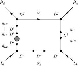
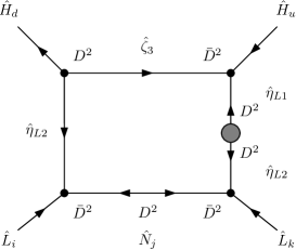
Figure 15: Supergraphs for leading order $B_{\eta_{L}}$-term (grey blobs) contribution to $LLH_{u}H_{d}^{\dagger}$.

To be precise, the $\mu_{L}$-independent $B_{\eta_{L}}$-term contributions coming from the first and second supergraphs add up to

$$\lim_{M_{N}=\mu_{L2}=\mu_{s3}}\Big{(}M_{N}\mu_{L2}^{2}E_{0}+M_{N}\Big{[}D_{0}+\mu_{L2}^{2}E_{0}\Big{]}\Big{)}\int d^{4}\theta\,D^{2}\left(\frac{\hat{X}^{\dagger}\hat{X}}{M^{2}_{X}}\right)_{B_{\eta_{L}}}\hat{L}\hat{L}\hat{H}_{u}\hat{H}_{d}^{\dagger}=0\,,$$ (79)

respectively, and where $D_{0}$ and $E_{0}$ are the following scalar one-loop integrals evaluated at $p_{\text{ext}}=0$: $D_{0}(...,M_{N}^{2},\mu_{L2}^{2},\mu_{s3}^{2},\mu_{L2}^{2})$ and $E_{0}(...,M_{N}^{2},\mu_{L2}^{2},\mu_{L2}^{2},\mu_{s3}^{2},\mu_{L2}^{2})$, respectively. $\hat{X}^{\dagger}\hat{X}$ is a ${\cancel{\text{SUSY}}}$ spurion insertion (cf. Eq. (42)). The remainder of the second supergraph generates the $\mu_{L}$-dependent $B_{\eta_{L}}$-term contribution:

$$M_{N}E_{0}\int d^{4}\theta\,\bar{D}^{2}D^{2}\left(\frac{\hat{X}^{\dagger}\hat{X}}{M^{2}_{X}}\right)_{B_{\eta_{L}}}\hat{L}\hat{L}D^{2}\hat{H}_{u}\hat{H}^{\dagger}_{d}\supset|\mu_{L}|^{2}B_{\eta_{L}}M_{N}E_{0}\,LLH_{u}H^{\dagger}_{d}\,.$$ (80)

Appendix E Radiative renormalisable couplings in SUSY

In this appendix we show that, by relying just on the renormalisability of the superpotential, some four-scalar couplings can be genuinely radiative.

Let $\hat{X}_{i}$ be a chiral scalar superfield of components $\phi_{i}$, $\chi_{i}$ and $F_{i}$. In each statement we increase $i$ whenever a field/superfield is introduced that does not need to have the identity of a previously introduced field/superfield. For instance, when an $F_{i}$ is used, we say that it contains some $\phi$’s labelled by increasing the counter $i$. In this way no a priori assumption is made regarding the form of the superpotential.

The only radiative possibility for renormalisable spinor-scalar interactions is (schematically)

$$\frac{1}{M}\int d^{4}\theta\,\hat{X}^{\dagger}_{1}\hat{X}_{2}\hat{X}_{3}\supset\frac{1}{M}F^{\dagger}_{1}\chi_{2}\chi_{3}\supset\phi_{4}\chi_{2}\chi_{3}\,.$$ (81)

This means that $\hat{X}_{2}\hat{X}_{3}\hat{X}_{4}$ is symmetric and, since it is renormalisable, allowed in the superpotential. Thus, there is a tree-level contribution to $\phi_{4}\chi_{2}\chi_{3}$. Regarding three-scalar interactions, the possibilities are

$$\begin{aligned} &\int d^{4}\theta\,\hat{X}^{\dagger}_{1}\hat{X}_{2}\supset F^{\dagger}_{1}F_{2}\supset M\phi_{3}\phi_{4}\phi^{\dagger}_{5}\,,\\ &\frac{1}{M}\int d^{4}\theta\,\hat{X}^{\dagger}_{1}\hat{X}_{2}\hat{X}_{3}\supset\frac{1}{M}F^{\dagger}_{1}F_{2}\phi_{3}\supset M\phi_{4}\phi^{\dagger}_{5}\phi_{3}\,,\end{aligned}$$ (82)

where both say that $\hat{X}_{2}\hat{X}_{3}\hat{X}_{4}$ is symmetric, and thus allowed in the superpotential. In addition, the first necessitates $\hat{X}_{1}\hat{X}_{3}\hat{X}_{4},\hat{X}_{2}\hat{X}_{5}\subset\mathcal{W}$, while the second necessitates $\hat{X}_{2}\hat{X}_{5},\hat{X}_{1}\hat{X}_{4}\subset\mathcal{W}$. Hence, in both cases there is a tree-level contribution to $\phi_{3}\phi_{4}\phi^{\dagger}_{5}$ once $F_{2}$ is integrated out. Regarding four-scalar interactions, we have

$$\begin{aligned} \text{(a)}&&&\int d^{4}\theta\,\hat{X}^{\dagger}_{1}\hat{X}_{2}\supset\phi_{3}\phi_{4}\phi^{\dagger}_{5}\phi^{\dagger}_{6}\,,\\ \text{(b)}&&&\frac{1}{M}\int d^{4}\theta\,\hat{X}^{\dagger}_{1}\hat{X}_{2}\hat{X}_{3}\supset\phi_{4}\phi^{\dagger}_{5}\phi^{\dagger}_{6}\phi_{3}\,,\\ \text{(c)}&&&\frac{1}{M}\int d^{4}\theta\,\hat{X}^{\dagger}_{1}\hat{X}_{2}\hat{X}_{3}\supset\phi_{4}\phi_{5}\phi^{\dagger}_{6}\phi_{3}\,,\\ \text{(d)}&&&\frac{1}{M^{2}}\int d^{4}\theta\,\hat{X}^{\dagger}_{1}\hat{X}_{2}\hat{X}_{3}\hat{X}_{4}\supset\phi_{5}\phi^{\dagger}_{6}\phi_{3}\phi_{4}\,,\\ \text{(e)}&&&\frac{1}{M^{2}}\int d^{4}\theta\,\hat{X}^{\dagger}_{1}\hat{X}_{2}\hat{X}^{\dagger}_{3}\hat{X}_{4}\supset\phi_{5}\phi^{\dagger}_{6}\phi^{\dagger}_{3}\phi_{4}\,.\end{aligned}$$ (83)

(a) and (b) entail a tree-level contribution. (c) and (d) have tree-level contributions if and only if there exists a representation $\hat{Y}\sim\hat{X}_{2}$ such that $\hat{Y}\hat{X}_{3}\hat{X}_{4}\hat{X}_{5}$ is generated at tree-level; in the case of (c), this happens if $\hat{X}_{1}$ is massive. (e) has a tree-level contribution if and only if the model contains a representation $\hat{Y}$ such that

$$\hat{Y}\hat{X}_{4}\hat{X}_{5},\hat{Y}\hat{X}_{3}\hat{X}_{6}\subset\mathcal{W}~{}~{}\text{or}~{}~{}\hat{Y}\hat{X}_{1}\hat{X}_{3},\hat{Y}\hat{X}_{2}\hat{X}_{4}\subset\mathcal{W}\,,$$ (84)

corresponding to the tree-level exchange of $F_{Y}$ or $\phi_{Y}$, respectively. If former’s case $\hat{Y}$ has a mass term, there is also a contribution due to an exchange of $\bar{\phi}_{Y}$ and the sum of the two gives

$$\phi^{\dagger}_{3}\phi^{\dagger}_{6}\frac{-\Box}{-\Box-M^{2}_{Y}}(\phi_{4}\phi_{5})\,.$$ (85)

For an easier understanding of the “only if” part of these assertions, we show in Fig. 16 all possible realisations of tree-level $\phi^{\dagger}\phi^{3}$ and $(\phi^{\dagger}\phi)^{2}$ under the assumption of a renormalisable superpotential. We use auxiliary fields, shown as dotted lines with an arrowhead, to make clear the holomorphy of the superpotential.

Figure 16: All possible tree-level topologies of $\phi^{\dagger}\phi^{3}$ and $(\phi^{\dagger}\phi)^{2}$ under the assumption of a renormalisable superpotential. Exchanges of $F_{Y}$, $\bar{\phi}_{Y}$ ($F_{Y}$-induced) and $\phi_{Y}$, as mentioned in the text, correspond to the last three diagrams.

To conclude, four-scalar couplings coming from (c), (d) or (e) are possible radiative couplings in a supersymmetric setting.

Appendix F Model example

Our conventions regarding $SU(2)_{L}$ contractions in the superpotential of Eq. (47) are fully specified by the following. Reading each term from left to right, let $\hat{A}$ be the first doublet superfield and $\hat{B}$ the second, and let $\epsilon_{12}=1$ be the totally anti-symmetric tensor. Then,

$$\begin{aligned} \mathbf{3}\otimes\mathbf{2}\otimes\mathbf{2}\supset\mathbf{1}:&~{}~{}&&\hat{\Delta}\hat{A}\hat{B}:=\hat{\Delta}^{\alpha}\underline{\hat{A}}{}^{a}T^{\alpha}_{ab}\hat{B}^{b}=\hat{\Delta}^{\alpha}\hat{A}^{a}(\epsilon T^{\alpha})_{ab}\hat{B}^{b}\,,\\ &&&(\hat{\Delta}\hat{A}\hat{B})^{\dagger}:=\hat{\Delta}^{\dagger\alpha}\hat{B}^{\dagger a}T^{\alpha}_{ab}\underline{\hat{A}^{\dagger}}{}^{b}=\hat{\Delta}^{\dagger\alpha}\hat{B}^{\dagger a}(-T^{\alpha}\epsilon)_{ab}\hat{A}^{\dagger b}\,,\\ \mathbf{3}\otimes\mathbf{3}\supset\mathbf{1}:&&&\hat{\Delta}\hat{\overline{\Delta}}:=2\hat{\Delta}^{\alpha}\hat{\overline{\Delta}}{}^{\beta}\text{Tr}\left[T^{\alpha}T^{\beta}\right]\,,\\ \mathbf{2}\otimes\mathbf{2}\supset\mathbf{1}:&&&\hat{A}\hat{B}:=(\hat{A}\hat{B}):=\hat{A}^{a}\epsilon_{ab}\hat{B}^{b}\,,\end{aligned}$$ (86)

where $\underline{\hat{A}}{}^{a}:=-\epsilon_{ab}\hat{A}^{b}$.

Useful identities are

$$\begin{aligned} \left[\hat{L}^{a}_{i}(\epsilon T^{\alpha})_{ab}\hat{L}^{b}_{j}\right]\left[\hat{H}_{u}^{c}(\epsilon T^{\alpha})_{cd}\hat{H}_{u}^{d}\right]&=-\frac{1}{2}\left(\hat{L}_{i}\hat{H}_{u}\right)\left(\hat{L}_{j}\hat{H}_{u}\right)\,,\\ \left[\hat{L}^{a}_{i}(\epsilon T^{\alpha})_{ab}\hat{L}^{b}_{j}\right]\left[H_{u}^{c}(\epsilon T^{\beta}T^{\alpha})_{cd}H_{u}^{d}\right]&=\frac{1}{2}\left(\hat{L}_{(i}\hat{H}_{u}\right)\left[\hat{H}_{u}^{a}(\epsilon T^{\beta})_{ab}\hat{L}_{j)}^{b}\right]\,,\\ \left[\hat{L}^{a}_{i}(\epsilon T^{\alpha})_{ab}\hat{L}^{b}_{j}\right]\left[\hat{H}_{u}^{c}(\epsilon T^{\beta}T^{\alpha})_{cd}\hat{H}_{u}^{d}\right]\left[\hat{H}^{\dagger e}T^{\beta}_{ef}\hat{H}^{f}\right]&=\begin{aligned} &\frac{1}{4}\left(\hat{L}_{(i}\hat{H}_{u}\right)\left(\hat{H}_{u}\hat{H}\right)\hat{H}^{\dagger}\hat{L}_{j)}\\ &+\frac{1}{8}\left(\hat{L}_{i}\hat{H}_{u}\right)\left(\hat{L}_{j}\hat{H}_{u}\right)\hat{H}^{\dagger}\hat{H}\,,\end{aligned}\end{aligned}$$ (87)

where indices within $(~{})$ are symmetrised in a normalised way.

We define the following abbreviations for scalar one-loop integrals [39] evaluated at $p_{\text{ext}}=0$:

$$\begin{aligned} &C_{0}:=C_{0}(0,0,0,M^{2}_{X_{1}},M^{2}_{X_{2}},M^{2}_{X_{3}})\,,\\ &D_{0,0}:=D_{0}(0,0,0,0,0,0,M^{2}_{X_{1}},M^{2}_{X_{2}},M^{2}_{X_{3}},0)\,,\\ &D_{0,i}:=D_{0}(0,0,0,0,0,0,M^{2}_{X_{1}},M^{2}_{X_{2}},M^{2}_{X_{3}},M^{2}_{X_{i}})\,,\\ &E_{0,i}:=E_{0}(0,0,0,0,0,0,0,0,0,0,M^{2}_{X_{1}},M^{2}_{X_{2}},M^{2}_{X_{3}},M^{2}_{X_{3}},M^{2}_{X_{i}})\,,\end{aligned}$$ (88)

where $i=1,2,3$.

F.1 Dimension-7 $\text{OP}\in\text{OP}_{\nu}$

The supergraphs of Fig. 12 involving each of the $SU(2)_{L}\otimes U(1)_{Y}$ gauge vector superfields turn out to add up to an overall dependence in which all $M_{X_{i}}^{2}$ are equally weighed. This is due to a partial cancellation between upper and lower diagrams. Hence, the possibility of attaching $\hat{V}_{SU(2)_{L}}$ to either $\hat{X}_{1}/\hat{\overline{X}}_{1}$ or $\hat{X}_{2}/\hat{\overline{X}}_{2}$ simplifies to a multiplicative factor of $2$. We thus find that the effective Kähler potential contains

$$\frac{\mathbf{a}M_{X_{3}}C_{0}}{32\pi^{2}M_{\Delta}^{2}}D^{2}(\hat{L}^{a}\hat{L}^{b})\hat{H}_{u}^{c}\hat{H}_{u}^{d}\left[g^{\prime 2}\hat{V}_{U(1)_{Y}}\epsilon_{ac}\epsilon_{bd}+2g^{2}\hat{V}^{\alpha}_{SU(2)_{L}}\epsilon_{ac}(\epsilon T^{\alpha})_{db}\right]\,.$$ (89)

Hence, the effective Lagrangian contains

$$\frac{g^{2}\mathbf{a}M_{X_{3}}C_{0}}{32\pi^{2}M_{\Delta}^{2}}\left(\frac{1}{2c_{w}^{2}}\left(LH_{u}\right)\left(LH_{u}\right)\left[H^{\dagger}_{u}H_{u}+c_{2w}H^{\dagger}_{d}H_{d}\right]+\left(LH_{u}\right)\left(H_{u}H_{d}\right)H^{\dagger}_{d}L\right)\,.$$ (90)

The other supergraphs give

$$\begin{aligned} &-\frac{\mathbf{a}M_{X_{3}}}{32\pi^{2}M^{2}_{\Delta}}\sum_{i=1}^{2}|\lambda_{i}|^{2}(D_{0,3}+M^{2}_{X_{i}}E_{0,i})\int d^{4}\theta\,D^{2}(\hat{L}^{a}_{i}\hat{L}^{b}_{j})\hat{H}_{u}^{c}\hat{H}_{u}^{d}\hat{H}_{u}^{\dagger e}\hat{H}_{u}^{f}\epsilon_{ac}\epsilon_{bd}\delta_{ef}\\ &+\frac{\mathbf{b}M_{X_{3}}M_{X_{1}}M_{X_{2}}}{32\pi^{2}M_{\Delta}}\sum_{i=1}^{2}|\lambda_{i}|^{2}E_{0,i}\int d^{4}\theta\left(\hat{L}_{i}\hat{H}_{u}\right)\left(\hat{L}_{j}\hat{H}_{u}\right)\hat{H}^{\dagger}_{u}\hat{H}_{u}\end{aligned}$$ (91)

$$\begin{aligned} &&\supset&-\frac{\mathbf{a}M_{X_{3}}|\mu|^{2}}{16\pi^{2}M^{2}_{\Delta}}\sum_{i=1}^{2}|\lambda_{i}|^{2}(D_{0,3}+M^{2}_{X_{i}}E_{0,i})\left[\frac{1}{2}\left(LH_{u}\right)\left(LH_{u}\right)H^{\dagger}_{d}H_{d}-\left(LH_{u}\right)\left(H_{u}H_{d}\right)H^{\dagger}_{d}L\right]\\ &&&+\frac{\mathbf{b}M_{X_{3}}M_{X_{1}}M_{X_{2}}\mu}{32\pi^{2}M_{\Delta}}\sum_{i=1}^{2}|\lambda_{i}|^{2}E_{0,i}\left(LH_{u}\right)\left(LH_{u}\right)\left(H_{u}H_{d}\right)\,.\end{aligned}$$ (92)

F.2 Dimension-5 $\text{OP}\in\text{OP}_{\nu}$

Inspection of Tab. 2, Tab. 3, Tab. 4, Tab. 5 and Tab. 8 reveals that, up to order $3$ in soft-${\cancel{\text{SUSY}}}$, there are $22$ terms contributing to $LLH_{u}H_{u}$ ($3$ of them proportional to $\bar{\lambda}_{X}$), $10$ terms to $LLH_{u}H^{\dagger}_{d}$ and $1$ to $LLH_{d}^{\dagger}H_{d}^{\dagger}$. To be specific, their contribution to the effective Lagrangian reads

$$-\frac{\lambda_{1}\lambda_{2}}{32\pi^{2}M_{\Delta}^{2}}\Bigg{(}\Bigg{[} \lambda^{*}_{X}M_{X_{3}}\Bigg{(}\begin{aligned} &\sum_{i=1}^{2}\left[(m_{\text{soft}}^{2})_{X_{i}}(C_{0}+M_{X_{i}}^{2}D_{0,i})+(m_{\text{soft}}^{2})_{\overline{X}_{i}}M_{X_{i}}^{2}D_{0,i}\right]\Bigg{.}\Bigg{.}\Bigg{.}\\ &+\left[(m_{\text{soft}}^{2})_{X_{3}}+(m_{\text{soft}}^{2})_{\overline{X}_{3}}\right](C_{0}+M_{X_{3}}^{2}D_{0,3})+A^{*}_{X}(A_{1}+A_{2})C_{0}\Bigg{)}\end{aligned}$$

$$-\bar{\lambda}_{X}M_{\Delta}\Bigg{(}M_{X_{3}}(B_{X_{1}}M_{X_{2}}D_{0,1}+B_{X_{2}}M_{X_{1}}D_{0,2})+B_{X_{3}}M_{X_{1}}M_{X_{2}}D_{0,3}\Bigg{)}$$

$$+\lambda^{*}_{X}(A_{1}+A_{2})\Bigg{(}M_{X_{3}}\sum_{i=1}^{2}B_{X_{i}}M_{X_{i}}D_{0,i}+B_{X_{3}}(C_{0}+M_{X_{3}}^{2}D_{0,3})-\frac{M_{X_{3}}B_{\Delta}C_{0}}{M_{\Delta}}\Bigg{)}$$

$$+\lambda^{*}_{X}A^{*}_{X}\Bigg{(}M_{X_{3}}\sum_{i=1}^{2}B_{X_{i}}M_{X_{i}}D_{0,i}+B_{X_{3}}M_{X_{3}}^{2}D_{0,3}\Bigg{)}\Bigg{]}H_{u}H_{u}$$

$$-2\mu^{*}\lambda^{*}_{X}\Bigg{[}\begin{aligned} &M_{X_{3}}\left(A^{*}_{X}C_{0}+\sum_{i=1}^{2}M_{X_{i}}B_{X_{i}}D_{0,i}-\frac{B_{\Delta}C_{0}}{M_{\Delta}}\right)+B_{X_{3}}\left(C_{0}+M_{X_{3}}^{2}D_{0,3}\right)\\ &+A^{*}_{X}M_{X_{3}}\Bigg{(}\begin{aligned} &\sum_{i=1}^{2}(m_{\text{soft}}^{2})_{X_{i}}D_{0,i}+\frac{1}{2}\left[(m_{\text{soft}}^{2})_{X_{3}}+(m_{\text{soft}}^{2})_{\overline{X}_{3}}\right]D_{0,3}\\ &-\frac{(m_{\text{soft}}^{2})_{\Delta}C_{0}}{M_{\Delta}^{2}}\Bigg{)}\Bigg{]}H_{u}H^{\dagger}_{d}\end{aligned}\end{aligned}$$

$$+(\mu^{*})^{2}\lambda^{*}_{X}A^{*}_{X}B_{X_{3}}D_{0,3}\,H^{\dagger}_{d}H^{\dagger}_{d}\Bigg{)}L\,\boldsymbol{\lambda_{L}}L\,.$$ (93)

These results have been confirmed by standard means of calculation, and further checked against algorithmic evaluations with FeynArts/FormCalc [41]. To generate the necessary model files we have used to our advantage FeynRule’s [42] support for superfields.

References

- [1] P. Minkowski, Phys. Lett. B 67 (1977) 421; M. Gell-Mann, P. Ramond and R. Slansky, “The Family Group in Grand Unified Theories,” in Sanibel Conference (1979), CALT-68-700, reprinted in hep-ph/9809459; M. Gell-Mann, P. Ramond and R. Slansky, in Complex Spinors and Unified Theories eds. P. Van. Nieuwenhuizen and D. Z. Freedman, Supergravity (North-Holland, Amsterdam, 1979), p.315 [Print-80-0576 (CERN)], reprinted in arXiv:1306.4669; T. Yanagida, in Proceedings of the Workshop on the Unified Theory and the Baryon Number in the Universe, eds. O. Sawada and A. Sugamoto (KEK, Tsukuba, 1979), p.95; S. L. Glashow, in Quarks and Leptons, eds. M. Lévy et al. (Plenum Press, New York, 1980), p.687; R. N. Mohapatra and G. Senjanović, Phys. Rev. Lett. 44 (1980) 912.
- [2] J. Schechter and J. W. F. Valle, Phys. Rev. D 22 (1980) 2227; R. N. Mohapatra and G. Senjanovic, Phys. Rev. D 23 (1981) 165; G. Lazarides, Q. Shafi and C. Wetterich, Nucl. Phys. B 181 (1981) 287; C. Wetterich, Nucl. Phys. B 187 (1981) 343; J. Schechter and J. W. F. Valle, Phys. Rev. D 25 (1982) 774.
- [3] S. Weinberg, Phys. Rev. Lett. 43 (1979) 1566.
- [4] V. N. Aseev et al. [Troitsk Collaboration], Phys. Rev. D 84 (2011) 112003 [arXiv:1108.5034 [hep-ex]].
- [5] M. Moresco, L. Verde, L. Pozzetti, R. Jimenez and A. Cimatti, JCAP 1207 (2012) 053 [arXiv:1201.6658 [astro-ph.CO]]; S. Riemer-Sorensen, C. Blake, D. Parkinson, T. M. Davis, S. Brough, M. Colless, C. Contreras and W. Couch et al., Phys. Rev. D 85 (2012) 081101 [arXiv:1112.4940 [astro-ph.CO]]; J. -Q. Xia, B. R. Granett, M. Viel, S. Bird, L. Guzzo, M. G. Haehnelt, J. Coupon and H. J. McCracken et al., JCAP 1206 (2012) 010 [arXiv:1203.5105 [astro-ph.CO]].
- [6] C. H. Lee, P. S. Bhupal Dev and R. N. Mohapatra, Phys. Rev. D 88 (2013) 9, 093010 [arXiv:1309.0774 [hep-ph]].
- [7] K. S. Babu, S. Nandi and Z. Tavartkiladze, Phys. Rev. D 80 (2009) 071702 [arXiv:0905.2710 [hep-ph]].
- [8] F. Bonnet, D. Hernandez, T. Ota and W. Winter, JHEP 0910 (2009) 076 [arXiv:0907.3143 [hep-ph]].
- [9] R. N. Mohapatra, Phys. Rev. Lett. 56 (1986) 561; R. N. Mohapatra and J. W. F. Valle, Phys. Rev. D 34 (1986) 1642; M. C. Gonzalez-Garcia and J. W. F. Valle, Phys. Lett. B 216 (1989) 360.
- [10] A. Zee, Phys. Lett. B 93 (1980) 389 [Erratum-ibid. B 95 (1980) 461]; A. Pilaftsis, Z. Phys. C 55 (1992) 275 [hep-ph/9901206]; P. S. B. Dev and A. Pilaftsis, Phys. Rev. D 86 (2012) 113001 [arXiv:1209.4051 [hep-ph]].
- [11] K. S. Babu, Phys. Lett. B 203 (1988) 132.
- [12] L. M. Krauss, S. Nasri and M. Trodden, Phys. Rev. D 67 (2003) 085002 [hep-ph/0210389]; K. Cheung and O. Seto, Phys. Rev. D 69 (2004) 113009 [hep-ph/0403003].
- [13] E. Ma, Phys. Rev. D 73 (2006) 077301 [hep-ph/0601225].
- [14] M. Aoki, S. Kanemura and O. Seto, Phys. Rev. Lett. 102 (2009) 051805 [arXiv:0807.0361 [hep-ph]]; M. Aoki, S. Kanemura and O. Seto, Phys. Rev. D 80 (2009) 033007 [arXiv:0904.3829 [hep-ph]].
- [15] M. Gustafsson, J. M. No and M. A. Rivera, Phys. Rev. Lett. 110 (2013) 21, 211802 [arXiv:1212.4806 [hep-ph]].
- [16] E. Ma, Phys. Rev. Lett. 81 (1998) 1171 [hep-ph/9805219].
- [17] P. Fileviez Perez and M. B. Wise, Phys. Rev. D 80 (2009) 053006 [arXiv:0906.2950 [hep-ph]].
- [18] F. Bonnet, M. Hirsch, T. Ota and W. Winter, JHEP 1207 (2012) 153 [arXiv:1204.5862 [hep-ph]].
- [19] S. P. Martin, Phys. Rev. D 61 (2000) 035004 [hep-ph/9907550].
- [20] J. M. Frere, M. V. Libanov and S. V. Troitsky, Phys. Lett. B 479 (2000) 343 [hep-ph/9912204].
- [21] N. Arkani-Hamed, L. J. Hall, H. Murayama, D. Tucker-Smith and N. Weiner, Phys. Rev. D 64 (2001) 115011 [hep-ph/0006312].
- [22] J. M. Frere and E. Ma, Phys. Rev. D 68 (2003) 051701 [hep-ph/0305155].
- [23] D. A. Demir, L. L. Everett and P. Langacker, Phys. Rev. Lett. 100 (2008) 091804 [arXiv:0712.1341 [hep-ph]].
- [24] F. R. Joaquim and A. Rossi, Phys. Rev. Lett. 97 (2006) 181801 [hep-ph/0604083]; F. R. Joaquim and A. Rossi, Nucl. Phys. B 765 (2007) 71 [hep-ph/0607298].
- [25] R. N. Mohapatra, N. Okada and H. -B. Yu, Phys. Rev. D 78 (2008) 075011 [arXiv:0807.4524 [hep-ph]].
- [26] P. Fileviez Perez, H. Iminniyaz, G. Rodrigo and S. Spinner, Phys. Rev. D 81 (2010) 095013 [arXiv:0911.1360 [hep-ph]].
- [27] R. Foot, H. Lew, X. G. He and G. C. Joshi, Z. Phys. C 44 (1989) 441.
- [28] A. Rossi, Phys. Rev. D 66 (2002) 075003 [hep-ph/0207006].
- [29] J. A. Casas, J. R. Espinosa and I. Navarro, Phys. Rev. Lett. 89 (2002) 161801 [hep-ph/0206276].
- [30] A. Brignole, F. R. Joaquim and A. Rossi, JHEP 1008 (2010) 133 [arXiv:1007.1942 [hep-ph]].
- [31] L. E. Ibanez, Phys. Lett. B 117 (1982) 403; A. B. Lahanas and D. Wyler, Phys. Lett. B 122 (1983) 258.
- [32] F. Borzumati, G. R. Farrar, N. Polonsky and S. D. Thomas, Nucl. Phys. B 555 (1999) 53 [hep-ph/9902443].
- [33] P. Batra and E. Ponton, Phys. Rev. D 79 (2009) 035001 [arXiv:0809.3453 [hep-ph]].
- [34] S. J. Gates, M. T. Grisaru, M. Rocek and W. Siegel, Front. Phys. 58 (1983) 1 [hep-th/0108200].
- [35] L. Girardello and M. T. Grisaru, Nucl. Phys. B 194 (1982) 65.
- [36] R. Franceschini and R. N. Mohapatra, Phys. Rev. D 89 (2014) 055013 [arXiv:1306.6108 [hep-ph]].
- [37] S. Bhattacharya, E. Ma and D. Wegman, Eur. Phys. J. C 74 (2014) 2902 [arXiv:1308.4177 [hep-ph]].
- [38] S. Kanemura, N. Machida, T. Shindou and T. Yamada, Phys. Rev. D 89 (2014) 1, 013005 [arXiv:1309.3207 [hep-ph]].
- [39] G. Passarino and M. J. G. Veltman, Nucl. Phys. B 160 (1979) 151; A. Denner, Fortsch. Phys. 41 (1993) 307 [arXiv:0709.1075 [hep-ph]]; R. Mertig, M. Bohm and A. Denner, Comput. Phys. Commun. 64 (1991) 345; We follow the conventions of: T. Hahn and M. Perez-Victoria, Comput. Phys. Commun. 118 (1999) 153 [hep-ph/9807565].
- [40] S. Kanemura, T. Shindou and T. Yamada, Phys. Rev. D 86 (2012) 055023 [arXiv:1206.1002 [hep-ph]]; S. Kanemura, E. Senaha, T. Shindou and T. Yamada, JHEP 1305 (2013) 066 [arXiv:1211.5883 [hep-ph]].
- [41] T. Hahn, Comput. Phys. Commun. 140 (2001) 418 [hep-ph/0012260].
- [42] A. Alloul, N. D. Christensen, C. Degrande, C. Duhr and B. Fuks, “FeynRules 2.0 - A complete toolbox for tree-level phenomenology,” arXiv:1310.1921 [hep-ph].