Uncovering Multiple Populations with Washington Photometry:
I. The Globular Cluster NGC 1851
Abstract
The analysis of multiple populations (MPs) in globular clusters (GCs) has become a forefront area of research in astronomy. Multiple red giant branches (RGBs), subgiant branches (SGBs), and even main sequences (MSs) have now been observed photometrically in many GCs, while broad abundance distributions of certain elements have been detected spectroscopically in most, if not all, GCs. UV photometry has been crucial in discovering and analyzing these MPs, but the Johnson U and the Stromgren and Sloan u filters that have generally been used are relatively inefficient and very sensitive to reddening and atmospheric extinction. In contrast, the Washington C filter is much broader and redder than these competing UV filters, making it far more efficient at detecting MPs and much less sensitive to reddening and extinction. Here we investigate the use of the Washington system to uncover MPs using only a 1-meter telescope. Our analysis of the well-studied GC NGC 1851 finds that the C filter is both very efficient and effective at detecting its previously discovered MPs in the RGB and SGB. Remarkably, we have also detected an intrinsically broad MS best characterized by two distinct but heavily overlapping populations that cannot be explained by binaries, field stars, or photometric errors. The MS distribution is in very good agreement with that seen on the RGB, with 30% of the stars belonging to the second population. There is also evidence for two sequences in the red horizontal branch, but this appears to be unrelated to the MPs in this cluster. Neither of these latter phenomena have been observed previously in this cluster. The redder MS stars are also more centrally concentrated than the blue MS. This is the first time MPs in a MS have been discovered from the ground, and using only a 1-meter telescope. The Washington system thus proves to be a very powerful tool for investigating MPs, and holds particular promise for extragalactic objects where photons are limited.
1. Introduction:
Globular clusters (GCs) have historically been considered quintessential Simple Stellar Populations, but a rapidly growing body of both spectroscopic and photometric work has shown that most, if not all, GCs are composed of multiple populations (MPs), with distinct chemical compositions and ages. For decades, low-resolution spectroscopy of limited samples in GCs has shown evidence for CN and CH abundance variations within some GCs (e.g., Hesser et al. 1976; Hesser et al. 1982), but establishing that these were MPs and not simply effects of stellar evolution required much more detailed evidence. MPs have now been observed photometrically in a large number of GCs including Omega Cen (Bedin et al. 2004), NGC 2808 (Piotto et al. 2007), NGC 1851 (Milone et al. 2008, hereafter M08; Han et al. 2009, hereafter H09; and Lee et al. 2009, hereafter L09), NGC 104, NGC 362, NGC 5286, NGC 6388, NGC 6656, NGC 6715 and NGC 7089 (Piotto et al. 2012), and M4 (Marino et al. 2008). In these clusters multiple red giant branches (RBGs), sub giant branches (SGBs), or even main sequences (MSs) have been detected. Additionally, using 8-meter class telescopes with multi-object spectrographs, studies of large samples of GC stars at high resolution and signal to noise are now common and show that GCs have intrinsically broad abundance ranges in many elements (e.g., Carretta et al. 2011a for NGC 1851). The Na:O anticorrelation is the best studied characteristic of GC abundance spreads, and it has been found in virtually all clusters that have been observed with high-quality spectra of large samples of stars (Carretta et al. 2010). However, recent observations of Ruprecht 106 (Villanova et al. 2013), traditionally regarded as a GC due to its mass, age, metallicity, etc., found that it is the first such object that does NOT exhibit an anticorrelation or even an abundance spread in Na or O, or indeed any other element, although the sample size is small and more stars are needed to consolidate this result.
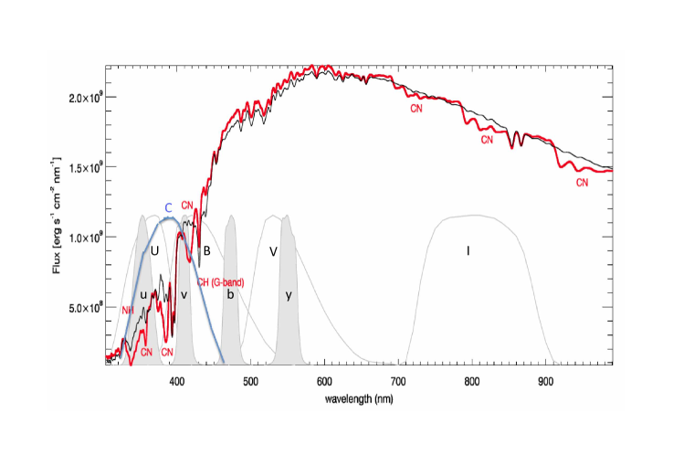
The interplay between good photometric and spectroscopic data has been crucial in uncovering MPs. Clearly, spectroscopic data are superior when there exists a large enough sample of stars observed at high resolution and signal to noise, enabling the determination of detailed abundances for a variety of elements. However, this technique is large-telescope-time intensive. Photometry enjoys a hefty advantage in this respect, allowing much larger samples covering a wider range of evolutionary stages. Furthermore, it provides the atmospheric parameters required for follow up determination of spectroscopic abundances. In order to properly identify MPs photometrically, the choice of filters is paramount. To date, the key has been using a combination of filters that include a UV bandpass. Several studies, especially Sbordone et al. (2011) and Carretta et al. (2011b), have now shown that realistic abundance differences in the CNO elements, as expected between MPs, greatly affect UV filter bandpasses because of the strong CN, CH, and NH molecular bands present (Figure 1). In contrast, the redder optical filters are much less affected. Because these elements and their variations are representative of MPs, a UV filter is now considered crucial in order to detect MPs. The Johnson U, Stromgren u, or Sloan u filters have been used for all previous ground-based detections of MPs with UV photometry, but all of these filters suffer serious limitations. They are notoriously inefficient and are confined to a wavelength range that is very sensitive to both interstellar and atmospheric extinction. Therefore, they require a significant amount of large telescope time to observe most GCs well, giving up a large part of the efficiency advantage that photometry enjoys over spectroscopy.
The Washington photometric system (Canterna 1976) was designed (Wallerstein & Helfer 1966) to derive an accurate photometric temperature and metallicity for late-type giant stars using broad band filters. The and (Temperature) filters are very similar to , providing a temperature index given by the color which is very similar to . The M (Metallicity) filter, centered near 5000 Å, combined with an appropriate comparison bandpass such as , yields a metallicity indicator. Finally, at the time the system was being setup, the phenomenon of CN and CH variations within GCs was being discovered (e.g. Hesser et al. 1976) and it was realized that the addition of another filter designed to measure the CN/CH strength independently of the metallicity would be of great use in disentangling these two abundances. Thus, the C (Carbon) filter was introduced, specifically to search for MPs. To our knowledge, this was the first and still only such filter so designed. In order to maintain the broadband characteristics of the system, the filter needed to cover a wide wavelength range that included significant CN and CH bands. A design goal was to include both the UV CN band near 3600 Å as well as the CH G-band near 4300 Å. As shown in Figure 1, the Washington C filter covers the same bandpasses and molecular bands as the other UV filters used to uncover MPs, and in fact more of these latter than any other competitor. It is also both much broader (FWHM 1000 Å) and centered significantly redward (3900 Å) of the other filters (see Table 1), making it much more efficient and less reddening and extinction sensitive. It even includes some sensitivity to the NH band at 3360 Å. Note that C has a very similar blue response as Johnson U but is centered 300 Å redder and retains significant sensitivity to beyond 4500 Å, far beyond the red cutoff of U. The peak transmission is also higher in C than the other filters. It is thus much faster (typically 3 times faster at obtaining the same S/N) than U and is many times more efficient than Stromgren or Sloan u, especially in red giants.
| Filter | Central | FWHM () | Peak Transmission | Source |
| Johnson U | 3570 | 650 | 72.47% | 1 |
| Washington C | 3850 | 1075 | 83% | 1 |
| SDSS u | 3600 | 400 | 65.49% | 1 |
| Stromgren u | 3537 | 278 | 38% | 2 |
The Washington system has been used for a wide variety of studies. Originally (Canterna 1976), metallicity determinations were based on a mean of the abundances derived from both the M and C filters as long as they were in good agreement. If there was a significant difference, the M metallicity was used and the star was labeled as having a CN/CH excess. This led to the discovery of a number of such stars, including the first extragalactic example (Canterna and Schommer 1978). Subsequently, Geisler (1986) discovered that the metallicity sensitivity of the C filter was superior to that of the M filter and recommended that future studies preferentially utilize the C filter for measuring metallicity. Indeed, this filter is sensitive to both CN/CH as well as traditional metal abundance because the bandpass also includes such features as the Ca II H and K lines and a series of strong Fe I lines spanning from 3400 to 4400 Å. Thus, the ability of the system to search for MPs was never fully exploited, despite its clear advantages in terms of efficiency and specific design for uncovering MPs.
Recently, a C-filter equivalent, F390W, has been added to the WFC3 filter complement aboard HST. This filter has indeed been utilized in MP studies, e.g. Bellini et al. 2013, and proven quite successful in this regard. However, such studies have not recognized or treated this as the Washington C filter. To our knowledge, the only relevant study to test this filter as the Washington C filter is a very recent one by Ross et al. (2014), where they tested the ability of various HST/WFC3 filters to derive photometric metallicities in five well studied galactic star clusters. They found the F390W filter is both the most efficient and also provides the second-best metallicity index after the F390M filter, which is unfortunately 4.5 times narrower. This study proves that the C filter is indeed very metallicity sensitive but does not demonstrate its potential for the MP phenomenon. Likewise, there have been no ground-based studies with the Washington system investigating its utility in this regard.
Given the above, we felt an initial ground-based study to investigate the ability of the Washington system to uncover MPs in Galactic GCs was well-motivated. Our initial target is NGC 1851. NGC 1851 is a particularly interesting cluster in many respects. Photometrically, it displays two RGBs (H09) and SGBs (M08; H09), and it has both a red horizontal branch (RHB) and a blue horizontal branch (BHB), which is not commonly seen in GCs. A great advantage for studying this cluster is its very low reddening of E(B-V) = 0.02 (Harris 1996), meaning that the potential complicating effects of variable reddening can be ignored (NB: ). Spectroscopically, the two RGBs observed in NGC 1851 typically exhibit different abundances in a variety of elements, most strikingly in Na, Ba, and N (Villanova et al. 2010, hereafter V10; Carretta et al. 2011a, hereafter Ca11; Carretta et al. 2014, hereafter Ca14), and the two SGBs appear to correspond to high and low Ba abundances (Gratton et al. 2012a). Therefore, abundance differences likely play an important if not dominant role in creating the separate sequences. The details for several of these key abundance differences are still debated. For example, V10 find that in 15 RGB stars the total C+N+O content shows no significant variation, while in a more limited sample of 4 giants Yong et al. (2009) find that the C+N+O content may vary by up to a factor of 4. Additionally, it has been argued that these two populations show evidence of different radial distributions by Zoccali et al. (2009) and Ca11, but both Milone et al. (2009) and Olszewski et al. (2009) have argued that there are still two sequences in the SGB at large radii with no statistically significant variations in the number ratios of the two populations with increasing radii. A further intriguing property of NGC 1851 is that it is one of the few GCs that possesses an apparent real spread in the heavy elements (e.g., Fe), not just in the light elements (Ca11). Theories to explain the MPs in NGC 1851 include: 1) an initial population formed and ejecta from its high-mass stars, including SNe, polluted the remaining gas. Soon after (1 Gyr), a second population formed from the polluted gas that was not expelled from the cluster (see M08, Ventura et al. 2009, and Joo & Lee 2013). 2) There was a merger of two GCs of slightly different age and composition (see Ca11).
This paper is the first in our survey of a sample of southern GCs using the Washington filters to investigate MPs. It is organized as follows: In Section 2 we discuss our observed data and methods of analysis. In Section 3 we discuss our photometric results and analyze in general what can be accomplished with them for studying multiple stellar populations in GCs using relatively little telescope time. In Section 4 we search for multiple MSs using our photometry. In section 5 we discuss in more detail the structure we observed in the red HB. In Section 6 we analyze potential differences in the radial distributions of the two populations. Lastly, in Section 7 we summarize our results and conclusions, and we point in several interesting directions for future analysis.
2. Observations and Analysis:
In order to demonstrate the efficiency of the Washington system in MP studies, we decided to use a 1-meter class telescope. Our observations of NGC 1851 were performed at the SWOPE 1-meter telescope at Las Campanas Observatory using the SITe#3 detector with 2048x3150 pixels at 0.435”/pixel and a field of view of 14.9x22.8 arcminutes. Both the R and T2 observations were performed during grey time on October 21, 2011 with one short C image taken that night before the Moon rose, and the remainder of the C observations were performed before the Moon rose on October 25, 2011. Note that Geisler (1996) has shown that the filter is an accurate and much more efficient substitute for the Washington filter. Both nights were determined to be photometric based on a series of observations of Geisler (1996) standard star fields. All of the R and T2 observations plus the single C image from October 21, 2011 had a FWHM of 0.95” to 1.05”, while the remaining C observations from October 21, 2011 had a FWHM of 1.5” to 1.95”. A total of 2 short C (300 seconds each), 9 long C (1200 seconds each), 1 short R (100 seconds), 3 long R (400 seconds each), 1 short T2 (300 seconds), and 3 long T2 (1200 seconds each) images were obtained, giving a total of 11,400 seconds for C, 1300 seconds for R, and 3900 seconds for I. In comparison, the Johnson UVI observations of H09 had a total exposure time of 5239 seconds on the Blanco 4-meter telescope (versus our 1-meter). Scaling the total exposure times by the aperture of the telescopes gives that this is effectively 5 times more telescope time. In comparison to the Stromgren observations of Lee et al. (2009), they had a total exposure time of 49,710 seconds (nearly 14 hours) on the SMARTS 1-meter telescope, which is 3 times more telescope time.
Standard IRAF tasks were used to process the data. Based on the detailed tests from Hamuy et al. (2006), we have adopted their non-linearity corrections for SITe#3. We also took a series of images to test for shutter corrections of the detector, but we found that if we corrected the shutter test images for the adopted non-linearity of the detector, no significant shutter correction was necessary. Since the NGC 1851 field is crowded, DAOPHOT was first applied independently in each image to a sample of bright and isolated stars to determine a first approximation for a quadratically-varying PSF. This initial PSF was then applied to subtract all neighboring stars from a larger sample of PSF stars (200 stars), which were used to determine a final quadratically-varying PSF (Stetson 1987). These final PSFs were applied with ALLFRAME to self-consistently measure the photometry of all images simultaneously (Stetson 1994). Aperture corrections were determined by comparing the PSF photometry of bright (but unsaturated) stars to their aperture photometry after all nearby-neighbor stars had been subtracted. Stars spanning the entire field were used to test for spatial dependence of the correction, but it was found to be uniform across the field in all filters. Additionally, several cuts were applied to the photometry based on the magnitude error, the chi-squared, and the sharpness value output by ALLFRAME. Individual star measurements with a magnitude error greater than 0.15, a chi-squared greater than 2.5, or an absolute value of sharpness greater than 1 were cut from the results. Lastly, the brightest stars that were affected by non-linearity of the detector, determined by where magnitude errors began to sharply increase with increasing brightness, were also cut.
The individual high-quality C, R and T2 magnitudes from ALLFRAME were first combined using DAOMASTER to create final C, R, and T2 instrumental magnitudes, which were then matched and combined to create a final list of stars with 2 to 3 of these filter magnitudes. The observations were transformed to the standard Washington system based on our observations of the standard star fields published in Geisler (1996), where the R magnitudes have been transformed to T1. For each night we had 8 standard observations in all 3 filters from 5 different standard fields. This gave a total of 79 standard stars in C, 70 in T1, and 69 in T2 that covered a broad range in UT, airmass, magnitude, and color. The RMS of the standardization was 0.024 for C, 0.016 and 0.017 for T1 when using a T1-T2 color term and a C-T1 color term, respectively, and 0.013 for T2, indicating both nights were of excellent photometric quality. Both C and T2 were well behaved and only required linear color terms. T1 required a quadratic color term both nights, but this quadratic color term has consistently been found across multiple nights of photometric observations and is likely due to the difference in the width, but similar centers, of the T1 and R filters.
Due to the large pixel scale of the SITe#3 camera (0.435”/pixel), we found that the very good seeing on October 21, 2011 produced stars with FWHMs of only 2.1 pixels. This created minor undersampling issues with our PSF measurements that increased the errors of the R and T2 observations, which were all obtained on that night. Using in DAOPHOT and ALLFRAME a fitting radius 0.4 pixels smaller than the measured FWHM was shown to moderately improve the errors, so we have used those measurements to produce our R and T2 instrumental magnitudes. Conversely, the C observations that were predominantly performed on October 25 had FWHMs of 3 to 4 pixels, so the C photometry was not affected by the large pixels.
Spatial variations of the photometric zero-point are a common problem that can be caused, for example, by focus variations across the field, and to derive higher precision photometry we have corrected them. By generating a variety of color magnitude diagrams using our C, T1, and T2 photometry and the B and V photometry acquired through private communication with Momany Y. (observed at the 2.2m ESO with WFI camera), we have used the RGB and the upper MS to fit fiducials and test for spatial variations in the relative color distributions. This method is similar to that typically applied for correcting differential reddening, but we do not apply a reddening law. We can assume that all color variations are due to true photometric variations and not variable reddening because NGC 1851 has a very small reddening of only 0.02 (see Section 1). Comparisons between our own C, T1, and T2 photometry show that there are meaningful spatial variations with respect to each other while the comparisons of B and V show no significant spatial variations with respect to each other. Therefore, to determine the variations in our magnitudes we have used V as the reference magnitude by creating colors with our filters versus their V and have only used their V for our magnitude axis. We can assume that all resulting spatial variations in color are due to our photometry and correct it by fitting the smooth spatial variations and apply this correction directly to our magnitudes.
The magnitude of the final corrections in each filter are typically or order 0.015 in C and 0.02 in both T1 and T2 and symmetric around zero. The corrections are comparable in magnitude across a majority of the field, but it should be noted that near only the northern edge of the image the corrections quickly become larger in all filters, being of order 0.06 in C and 0.05 in both T1 and T2. This variation at the northern edge is not of major concern considering the detector spans nearly 23 arcminutes along this axis and members of the centrally placed NGC 1851 will be very sparse near this edge. The independently corrected C and T1 magnitudes are both self-consistent with each other and show consistency in all magnitude ranges across the full field of view. However, the T2 magnitudes show spatial variations that are moderately inconsistent between the brighter and the fainter stars. We have chosen to correct these spatial variations differently for the brighter (T218) and fainter stars (T218) in T2. The source for these inconsistencies at differing magnitudes is uncertain, but it is possibly related to the minor fringing that occurs only in the T2 images. We did not have appropriate reference images to fully correct this minor fringing, but our spatial corrections will have also corrected its largest effects while the small scale fluctuations will have only introduced minor but not insignificant additional T2 errors. With this greater photometric uncertainty, we will still present our T2 photometry in this paper, but will also supplement our photometry with the B and V photometry of Momany Y. (private communication) to provide additional non-UV magnitudes. As a further constraint, we will not base any conclusions on characteristics seen only in color-magnitude diagrams (CMDs) containing T2, and will show that all characteristics observed using the T2 magnitudes are qualitatively consistent with the other comparable filter combinations.
For our final photometry, see Table 2 for an example, we have also applied a strict cut of our data near the core because both the spatial variations of the errors and our measurement tests of artificial stars show that crowding begins to affect an increasingly large fraction of the stars that are within 2 arcminutes of the center. The effects of crowding are not reliably represented by the ALLFRAME determined photometric error but are better represented by the resulting of the multiple measurements of each star. Therefore, each star near the center has been cut unless it has been measured multiple times in each filter and the resulting of the multiple measurements is 0.02 in both filters. This removes stars affected by crowding without removing the bright and centrally concentrated RGB stars that are still well measured near the center. Additionally, because we only have one available short T1 image, no stars brighter than a T1 of 15 will have multiple T1 detections. Therefore, for these stars we only require that they have multiple C detections and a resulting of less than 0.02. This effect from crowding in the core prevents us from having any overlap in our final sample and the proper motion sample of M08, where they looked at the SGB and MS in the central 2.7 arcminutes. However, their analysis does demonstrate that for NGC 1851 the field-star contamination is quite minor, as expected from its galactic latitude of -35 degrees.
| ID | X | Y | C | C Err | C Disp | T1 | T1 Err | T1 Disp | T2 | T2 Err | T2 Disp | C Count | T1 Count | T2 Count |
| 16798 | 1330.59 | 1083.73 | 15.971 | 0.005 | 0.004 | 12.833 | 0.016 | 0 | - | - | - | 4 | 1 | 0 |
| 16928 | 1274.17 | 1675.08 | 16.861 | 0.005 | 0.008 | 15.738 | 0.015 | 0.006 | - | - | - | 4 | 3 | 0 |
| 6984 | 633.17 | 1725 | 17.868 | 0.004 | 0.014 | 16.304 | 0.007 | 0.007 | 15.811 | 0.012 | 0.013 | 11 | 4 | 4 |
| 2832 | 1295.54 | 1435.55 | 18.55 | 0.004 | 0.017 | 17.228 | 0.01 | 0.009 | 16.728 | 0.014 | 0.012 | 10 | 4 | 4 |
| 6953 | 1349.92 | 1721.71 | 18.757 | 0.005 | 0.013 | 17.831 | 0.017 | 0.008 | 17.41 | 0.023 | 0 | 11 | 4 | 2 |
| 6345 | 1194.57 | 1673.08 | 19.48 | 0.007 | 0.019 | 18.469 | 0.022 | 0.044 | 18.087 | 0.025 | 0.014 | 11 | 3 | 3 |
| 3760 | 1622.07 | 1513.54 | 19.657 | 0.004 | 0.015 | 18.664 | 0.009 | 0.002 | 18.26 | 0.012 | 0.006 | 11 | 4 | 4 |
3. Multiple Populations in the Red Giant Branch and Subgiant Branch:
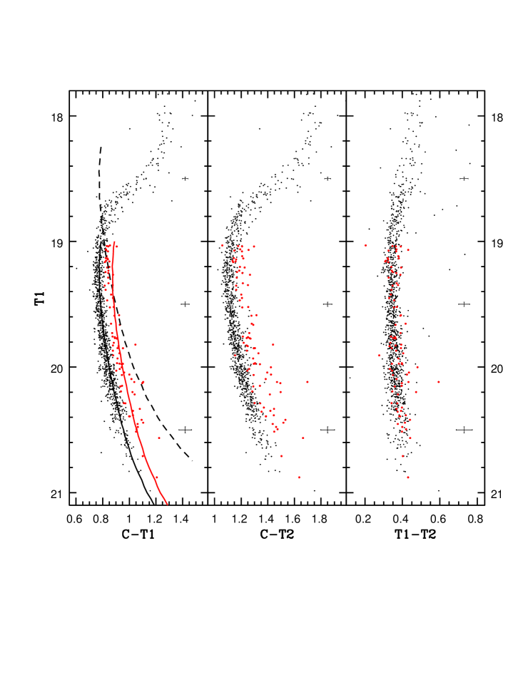
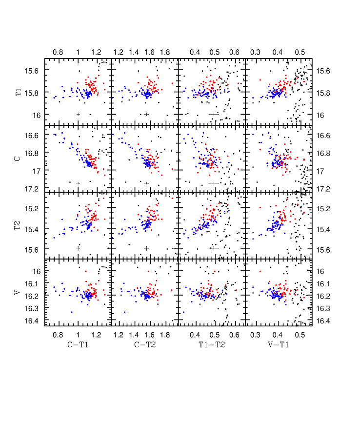
Figure 2 shows 4 CMDs from our final photometry. We show representative error bars on the side placed at each magnitude. These errors have been determined by both types of errors output by DAOMASTER: the combined photometric measurement error output by ALLFRAME and the based directly on the observational scatter across the multiple images. We typically find the photometric error dominates in the brightest stars but the observational scatter dominates in the fainter stars, and for each magnitude we take the largest of these two errors to be the better representation of its final error. For errors in color we add in quadrature the final errors from each input magnitude. Lastly, the representative errors shown in Figure 2 are found by taking the median error of all stars in a 1 magnitude range.
The brightest giants are saturated in our observations, so we have expanded our sample by taking advantage of the short photometric observations of NGC 1851 in C and T1 by Geisler & Sarajedini (1999) and the I observation from Momany Y. (private communication). Detailed comparisons of our observations to those of Geisler & Sarajedini (1999) show that their magnitudes are systematically brighter than ours by 0.006 in C and 0.029 in T1. Therefore, we have offset their results to be consistent and have used x symbols in the lower-right and upper-right panels of Figure 2 to distinguish their data. For expanding our T2 magnitudes, we have used the brightest 1000 stars (14.4T218.5) that have both our T2 and I from Momony to create a transformation relation. Because of the strong similarities between these two filters the relation is linear across this full magnitude range with little scatter, which allows us to extrapolate to stars brighter than T2=14.4 without likely introducing significant systematics. Using this relation we transform the I magnitudes for the brightest stars (T215) not in our sample to T2, and we mark this data in red in the upper-left and lower-left panels of Figure 2.
In the T1-T2 CMD (upper-left panel of Figure 2) there are no clear, separate branches visible, and the widths of the RGB and MS are similar to the representative errors displayed. This is consistent with previous ground-based studies that have shown that colors without a UV filter do not show either multiple branches or even a significantly broadened RGB. In contrast, things are very different in all CMDs including the C filter. We plot the C-T1 color both against T1 (upper right) and C (lower right). In both CMDs we see that in addition to the primary population there is a smaller but still significant population of SGB stars that are fainter than the primary SGB and a population of RGB stars that are redder than the primary RGB. The SGBs are shown more clearly in the insets. In Figure 3 we focus on the RGB and SGB in C-T1 versus C and for clarity color the two RGB branches. Both the fainter SGB and the redder RGB appear to be related and to create a continuous branch, a second population. These observations of a second population are similar to those of H09 using Johnson U and I. In direct comparison to H09, it should be noted that our second population stars do not appear to create as distinct or as well defined of a sequence as found in H09. They also appear to be less well defined than our primary population stars, suggesting that this is not the result of our observations having larger errors. Therefore, we cannot argue that in C the second population creates a photometrically distinct sequence from the primary SGB and RGB. Similar to C, however, the Stromgren observations in L09 also do not show a distinct second population sequence in the RGB.
In further comparison to the U-I versus U observations of H09, the mean color separation of the red and blue RGBs are quite similar to ours. Above the observed RGB bump, where the separation is the largest, both their observations and ours in C-T1 versus C show color separations of 0.25. In the lower RGB, while our color separation is more difficult to define here, we both find a color separation of 0.15. This significant change in color separation between the two populations between the upper and lower RGB is of interest. In our observations this change is more appropriately analyzed in C-T1 versus T1 (upper-right panel of Figure 2) because here the two populations are shifted in color but not magnitude. We see in C-T1 versus T1, in comparison to C-T1 versus C, that the true change in color separation between the upper and lower RGB is smaller but still is of significance. We expect a color separation increase, however, because the brighter giants are also increasingly cooler, leading to stronger molecular bands, giving that identical CNO variations will produce greater C magnitude differences.
Comparing the numbers of our red and blue RGB stars marked in Figure 3 gives that the number of the clearly distinct red RGB stars is only 13.6% of the total RGB population. This is significantly smaller than the 30% typically found for the second population when performing observations using Johnson filters (M08; H09), where the second populations in the SGB and RGB appear more distinctly separated. Therefore, this may be related to the more diffuse nature of this second population in our observations. This discrepancy and the second population’s color distribution will be discussed in more detail in Section 4.2. For simplicity we will refer to these distributions from now on as the red and the blue RGB branches, and the bright and the faint SGB branches.
In the C-T2 CMD we can still clearly see the separate branches of both the SGB and the RGB, but it is of interest that in this color we can no longer clearly detect the separate RHB branches observed with C-T1. Additionally, the two SGB and RGB branches are less defined. These differences may more be related to the increased errors for T2, rather than differing characteristics between T1 and T2, but these factors and the significantly shorter exposure times required for the T1 filter gives a clear advantage for the T1 over the T2 filter. Therefore, C-T1 will be our primary color for our analysis in the rest of this paper. But it remains ideal to still observe both T1 and T2 to verify the observed populations with both filters versus C and to compare these colors to the narrow RGB that is shown only in T1-T2.
We have further analyzed the significance of these photometric features in the RGB by comparing the color errors of the stars to their color differences from the RGB fiducial. We do this in 1 magnitude bins based on the median values of these parameters. Table 3 shows our results. In T1-T2, the ratio of width to errors ranges from 0.83 to 1.18, so the color errors are comparable to the observed width of the RGB and further strengthens our finding that there is no meaningful broadening in T1-T2. We perform a similar comparison for C-T1 using C-T1 versus T1. Across the full range of magnitudes the RGB appears to be intrinsically broad. In all 5 magnitude bins the width to error ratio is meaningfully larger than that seen in T1-T2, ranging from 1.5 to almost 3 . The comparison for C-T2 versus T2 also shows that on the RGB the width is significantly larger than the error, at 1.3 to 2.6 . The width of the broadened RGBs is the least significant in the faintest (hottest) RGB stars where the molecular bands will be the weakest. However, even at their weakest the RGB in C-T1 or C-T2 is still broader than that observed for T1-T2.
| Magnitude Range | Median Width | Median Error | Width to Error Ratio |
| RGB in T1-T2 versus T1 | |||
| 15-16 | 0.018 | 0.022 | 0.83 |
| 16-17 | 0.023 | 0.020 | 1.18 |
| 17-18 | 0.019 | 0.019 | 1.04 |
| RGB in C-T1 versus T1 | |||
| 13-14 | 0.035 | 0.023 | 1.50 |
| 14-15 | 0.042 | 0.016 | 2.69 |
| 15-16 | 0.039 | 0.014 | 2.77 |
| 16-17 | 0.032 | 0.017 | 1.95 |
| 17-18 | 0.028 | 0.018 | 1.55 |
| RGB in C-T2 versus T2 | |||
| 14.4-15 | 0.056 | 0.022 | 2.59 |
| 15-16 | 0.035 | 0.021 | 1.64 |
| 16-17 | 0.034 | 0.020 | 1.70 |
| 17-17.9 | 0.027 | 0.021 | 1.34 |
Figure 4 shows 4 additional CMDs based on combinations of our photometry and the B and V photometry. In the upper-left panel we look at V-T1 versus T1, which as expected is very similar to the T1-T2 versus T1 CMD from Figure 2. The more limited errors given for the B and V magnitudes do not allow us to create a detailed and consistent presentation of representative errors, but similar to what is seen in T1-T2 the RGB does not present multiple branches or appear meaningfully broadened in this color. In the lower-right panel we look at C-V versus C, and this CMD shares many similarities with both the C-T1 and C-T2 versus C CMDs from Figure 2. In particular, the RGB is heavily broadened with a more populous blue RGB and a sparser red RGB, and a faint SGB branch is also seen. The upper-right panel shows the very interesting B-T1 versus T1 figure. While the color does not involve the key C filter, the Johnson B filter overlaps with the C filter and still contains some of the important CN and CH bands (see Figure 1) that are believed to create the C magnitude variations. Consistent with this, the B-T1 versus T1 CMD exhibits a less significant but detectable population of red RGB stars that are similar to that seen in C-T1 versus T1. This leads us to the lower-left panel, which analyzes the C and B magnitudes using C-B versus C. Consistent with the previous observations, the RGB still is broadened, but less so than that observed in C-V. This is because both the C and B magnitudes are affected by the CNO variations, leading to a weaker but still detectable color difference between the two populations.
4. Multiple Populations on the Main Sequence:
4.1. Outer Annulus Analysis:
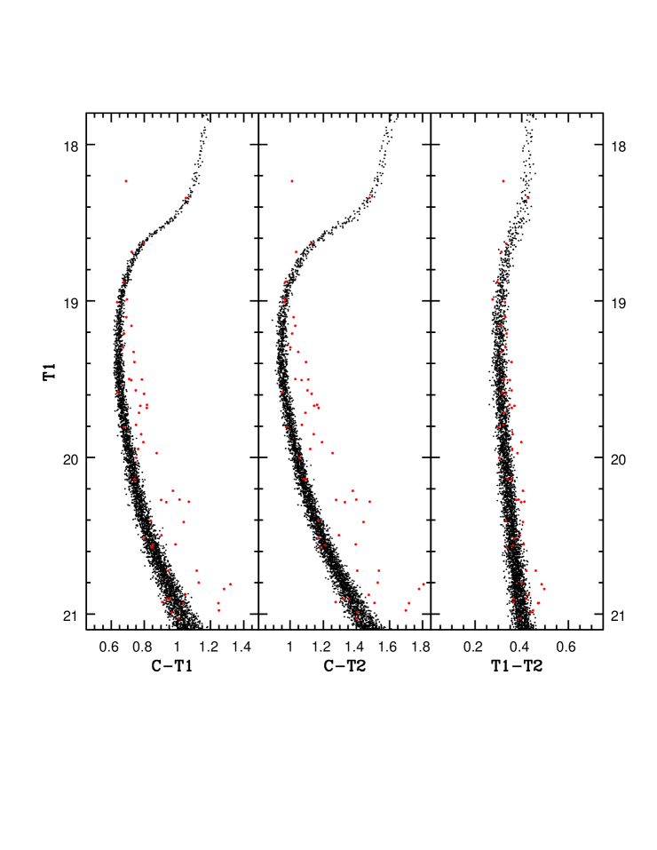
We can also search for MPs on the MS of NGC 1851, which have never been detected before, despite even being searched for in HST data (see M08). To limit our errors, we will first concentrate on stars well outside of the dense core but not apply too strict of an error cut or we will lose the faint MS stars. In Figure 5 we only show stars that have a C-T1 color error of 0.05 and that are in an annulus around the cluster center from 4 to 6.5 arcminutes. The half-mass radius from Harris (1996) is 0.52 arcminutes, giving that this is 7.7 to 12.5 half-mass radii from the center. Additionally, the representative error bars shown have been updated based on this subsample. We have plotted all of the colors versus T1 to increase the color difference between two potential populations. If we plotted versus C, a second redder population would also be shifted fainter, partly parallel with the MS, and decrease the apparent color difference at constant magnitude. Remarkably, in the left panel of Figure 5 we see clear signs for a broad MS with a substantial wing extending to the red that is not seen to the blue. This moderately redder MS population follows the same general shape as the primary population. Additionally, at the primary population’s turnoff this red population maintains its color separation and does not simply merge into the turnoff. Indeed, it appears to transition into the faint SGB that we have previously identified. To help illustrate this second population we have colored its likely members red in Figure 5, where we have based this solely on C-T1 and for stars with T119.
We must further analyze this red branch to test if it is a true second population or is simply a binary sequence, but we must also consider if it is a combination of both. In the left panel of Figure 5 we first characterize the primary MS with a solid-black line. We also illustrate a corresponding equal-mass binary sequence with a black-dashed line, which characterizes where the upper envelope of the binary sequence would be. This shows that the binaries would merge into the primary turnoff and then have their own turnoff at a brighter magnitude. Comparing to our data we find at the primary turnoff, even when considering errors, our observed second population still remains distinct and moderately red, and at fainter magnitudes the observed stars are increasingly too blue to be consistent with a binary sequence. Furthermore, there are a negligible number of stars that are consistent with a second brighter turnoff of binaries.
In Figure 6 we further illustrate the characteristics of a binary sequence using population synthesis of a population with a binary fraction of 3% using the TRILEGAL code (Girardi et al. 2005). We have input errors in this population synthesis based on our observed relation between photometric error and magnitude. To help distinguish the binaries in Figure 6 we have colored red all binaries with a mass fraction 0.6, while binaries of lower mass fraction will not be photometrically distinguishable from single stars. This population synthesis in C-T1 further shows that the binaries will appear relatively very red at fainter magnitudes, quickly begin to converge in color at brighter magnitudes and merge into the primary turnoff, and then have their own weakly populated turnoff at brighter magnitudes. In contrast to this, a true second population would be shifted redder in C-T1 but have no meaningful change in T1 magnitude. The median C-T1 color difference between these two branches is 0.096, and in Figure 5 the solid-red line demonstrates that this color shift is more comparable to the red MS stars. That the brighter stars are moderately bluer and the fainter stars moderately redder than this uniform color shift is further consistency with the two populations in the RGB stars (see Figure 2), which also exhibited changing color separations. In both cases the cooler stars, which will have stronger molecular bands, will create increased color separations at equivalent CNO abundance variations.
In the center and right panels of Figure 5 we will now analyze this observed second MS branch in other colors by taking the selected sample from C-T1 (colored red) and also coloring them red in these CMDs. In C-T2 (center panel of Figure 5) we see there is still a prominent redder population that is primarily composed of the same red stars observed in C-T1. The scatter of the two populations appears larger in this color, but this is consistent with T2’s moderately greater error. The median C-T2 color difference between the marked black and red populations is 0.109 (similar to the 0.096 in C-T1), and similarly shows the color difference between the two populations moderately increases in the fainter (cooler) stars. Comparing to the population synthesis for C-T2 (center panel of Figure 6), we see the same binary characteristics found in C-T1 and the same differences when compared to our observed second branch in C-T2. However, there is one key difference between the MS in C-T1 in comparison C-T2 that becomes readily apparent in their synthetic binary sequences: across the same T1 magnitude range the MS changes color in C-T2 more rapidly with decreasing magnitude, which greatly increases the apparent color separation between the single and binary sequences. Therefore, the greater observed color dispersion in the red branch of C-T2 (center panel of Figure 5) may be indicative of at least minor binary contamination, but overall because the color difference between the two populations in C-T1 and C-T2 are in agreement, this suggests that this is predominantly a true second population created by a shift in C magnitude.
We now mark these observed red-population stars in T1-T2 (right panel of Figure 5) and see that in this color there is no clear difference. The red-population stars observed in both C-T1 and C-T2 are distributed remarkably uniformly within this single sequence, and the median T1-T2 color difference is insignificant at 0.014. In contrast to this, the right panel of Figure 6 shows that in T1-T2 the binaries will still remain meaningfully redder than the single-star sequence. However, in our T1-T2 observations we do note a small number of color outliers are still seen in both populations. The total T1-T2 color distribution has a of 0.026 and we define the outliers as stars more than 2.5 from the central sequence. 2.6% of the primary population (black stars) are T1-T2 color outliers, with 1.1% being blue outliers and 1.5% being red outliers. In comparison a more significant 10.4% of the red population are outliers, but with only 2.3% being blue outliers and a much larger fraction of 8.1% being red outliers. Therefore, based on the small number statistics, in the primary population there is a comparable number of red and blue outliers, which are also comparable with the number of blue outliers in the red population. This suggests that 3-4% of both populations are true photometric outliers, non-members, or stars with abnormally large errors, which will approximately be distributed evenly between red and blue outliers. Correcting for this there remains an additional 6-7% of the red population that are red outliers in T1-T2. This small fraction of the red population (0.65% of the total population) may be true binaries that have a large mass ratio and will appear to be redder than the primary single-star population in all colors, while 93-94% of the red population remains strongly consistent with a second population of differing C magnitude.
If this second population of stars is not caused by a binary sequence, why do we not see a meaningful population of binaries in this outer annulus of NGC 1851? The recent definitive analysis of binary populations in GCs by Milone et al. (2012a) may provide an answer. They observed the MS in the central region (2.5 arcminutes from the center) with ACS/WFC in F606W and F814W, very similar to T1 and T2, giving a color that should make our two purported populations virtually indistinguishable in the MS. They observed that NGC 1851 only has a binary fraction of 0.80.3% for binaries with a mass ratio of greater than 0.5. Binaries with mass fractions of less than 0.5 were not able to be differentiated from single stars with their observations. Based on their models they estimate that NGC 1851 has a total binary fraction of only 1.60.6% in the observed central region. This is one of the lowest binary fractions of the 59 GCs they analyzed. Furthermore, their observations find that a majority of the observed GCs, including NGC 1851, have decreasing binary fractions at increasing distance from their center. This is consistent with expectations that binary systems, which dynamically act like a single star with mass equal to the sum of the binary components, will over time become more centrally concentrated in comparison to the less massive single stars. All of these factors suggest that in our observations of this outer annulus from 4 to 6.5 arcminutes, the binaries that would meaningfully contribute to a binary sequence (mass ratio0.5) is less than 1% of the total population. This is remarkably similar to our estimate from Figure 5 that in this outer annulus only 0.65% of our MS stars are consistent with large-mass-ratio binaries.
The number ratio for the red population shown in Figure 5 is 9.5%, which is comparable to the 13.6% found for the red RGB in comparison to the blue RGB in Section 3. Additionally, a comparable analysis of the SGB subsample shown in Figure 5 gives that the faint branch of the SGB is 12.7% of the total population. The agreement of the number ratios in all 3 regions of the CMD further strengthens the conclusion that this extended red population in the MS is a second population consistent with the one observed in both the SGB and RGB. However, it should be noted again that these number ratios are based on the photometrically distinct red stars, and more reliable color distributions and population ratios will be discussed in Section 4.2.
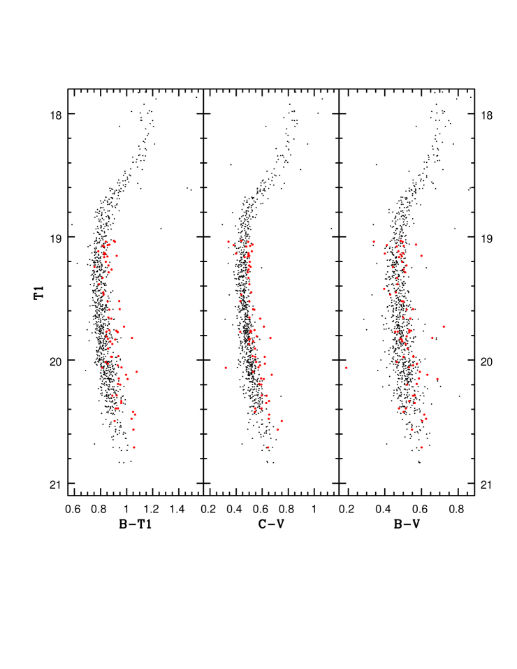
To further broaden our analysis, we can use the available B and V magnitudes. In Figure 7 we show the same sample of stars from Figure 5 (when B and V are available) using C-V, B-T1, and B-V. As in Figure 5 we again have marked the red population from C-T1 in all 3 CMDs. In the left panel of Figure 7 we see that in B-T1 the red MS population is not as distinct as in C-T1 or C-T2, but it is still significantly redder than the primary MS by 0.076. This is similar to what was seen with the RGB in B-T1 (Figure 4), which illustrated that in this color the two populations still exhibit a significant but smaller color difference to that seen in colors with C. As with the RGB, this is expected since CNO variations will also cause moderate differences in B magnitudes. The C-V color in the central panel is more surprising because even though the red MS still is consistently redder than the primary sequence, the difference is comparably weak at only 0.052. Lastly, in B-V we see that while there is not a large difference in color between the two populations, the red MS is still moderately redder than the primary MS by 0.030. This is relatively a minor difference but it is not insignificant. Both the central and right panels of Figure 7 suggest that for these two MS populations there may also be a weak difference in V magnitude, which results in a weaker than expected color difference when comparing to both C and B. Could this apparent difference in V magnitude for these two populations be indicative of additional effects beyond CNO variations for the two populations, e.g., possible differences in helium abundance, metallicity, or a large total C+N+O difference between these two populations?
This red MS population is very unlikely to be due to field stars, as it is centrally concentrated (see Section 6), and the field contamination is shown to be relatively minor in the proper motion analysis by M08. Stars photometrically consistent with binaries appear to only represent a minor portion (6-7%) of this red MS, consistent with this cluster’s small binary population (Milone et al 2012a). Furthermore, the effects of photometric error and crowding do not seem to be artificially creating this second branch (see the Appendix for detailed discussion of this). Therefore, Figures 5 to 7 provide strong evidence that these two MS branches are predominantly two populations of differing C magnitude with no meaningful difference in either T1 or T2, qualitatively consistent with the second population observed in both the SGB and RGB.
4.2. Full Field Analysis:
With strong evidence for two MS populations found in an outer annulus subsample of 1000 main-sequence stars, it is of great interest to look at a larger sample covering nearly the full field. Beginning with all stars from our original sample shown in Figure 2, which only placed a stringent error cut on the stars within 2 arcminutes of the center, we will focus on the 3162 MS stars with T119 and C-T1 color errors 0.05. With this large of a sample it is more informative to analyze the color distribution by taking a MS fiducial and creating a histogram of the color residuals in C-T1 versus T1. The left panel of Figure 8 shows this color distribution with bin sizes of 0.02, and we see that there is a significant sample of broadly distributed stars in the red wing that are not seen in the blue wing. A KMM mixture modeling test (Ashman et al. 1994) indicates that the probability this distribution is only a single Gaussian and not a bimodal distribution is essentially null. Initial attempts to fit these two possible populations using two offset Gaussians of equal sigma were not satisfactory. While the central peak is fit well by a Gaussian with a of 0.033, attempting to fit the redder population with a similarly narrow does a poor job of matching both the extended red wing and the blue wing.
Based on the analysis of synthetic CNO variations and abundances by Carretta et al. (2011b) and Ca11, they find that in colors involving Stromgren u the two RGB populations in NGC 1851 are not distinct sequences, similar to our C observations. In these papers they argue that the redder population is significantly broader in color than the blue population and the two populations are heavily overlapped, where the full redder population extends nearly as blue as the primary population. This suggests that our observed redder population may also only be the reddest wing of a broadly distributed population. Our synthetic analysis of the effects of CNO variations on the C magnitude, which will be discussed in detail in Cummings et al. (in prep.), shows the C filter also creates two heavily overlapping populations with a broader population extending well into the red. The left panel of Figure 8 shows our fit of the color distribution when assuming these population characteristics, with a large but narrow population with =0.031 and a smaller but significantly broader population with =0.075. This second population extends as blue as the first but also extends significantly redder creating the second population in the red wing. A clear advantage of this fit is that both the extremely blue and red stars are in agreement with the two Gaussians, which was not the case when using two slightly overlapping Gaussians of equal . For clarification this broad second population has partly been broadened further in this color distribution because its relative color difference between the primary population increases in the fainter (cooler) stars, so at any given magnitude its breadth will be smaller than 0.075 but still more significant than the narrow population with of only 0.031.
The peak heights and values of the blue and red distribution Gaussians are 556 and 0.031 and 99 and 0.075, respectively, giving that the broad and red MS is 30.1% of the total population. This is comparable to the ratio of 27.9% found for the percentage of blue HB to all HB stars, which are two far more reliably separated populations. This ratio is significantly larger than the population ratios found from Figure 3 and 5 of 13.6% for the red RGB, 9.5% for the red MS, and 12.7% for the faint SGB, but as suggested these smaller red populations analyzed are only the extreme red wing of the full broadly distributed second population. For independent comparison, M08 found that their fainter SGB was 30% of the total SGB population. Similarly, H09 found in their U-I observations that the secondary red RGB and faint SGB branches were also 30% of the total population.
To further test these significantly overlapping Gaussian fits, we have reanalyzed in C-T1 versus T1 the RGB from Figure 2 using an identical color distribution method. The right panel of Figure 8 shows the RGB color distribution for the 319 stars from 17.5T114, and we can fit it quite well with two Gaussians very similar to those we used for the MS. Again, the KMM test very strongly favors a bimodal over a unimodal Gaussian distribution. As discussed in Section 3, the color separation of the two RGB populations increases at brighter magnitudes, even more than that seen in the MS. Therefore, even with significantly lower color errors, the redder population requires an even broader Gaussian ( of 0.09 instead of 0.075). The two RGB populations are also more separated in color, with the Gaussian centers separated by 0.044 in the MS but by 0.064 in the RGB. Consistent with this difference, we will discuss in detail in Cummings et al. (in prep.) that CNO variations will cause differences in C magnitude in both the MS and RGB, but the differences is greater in the typically cooler RGB stars. Lastly, the peak heights and ’s of the blue and red distributions are 67.5 and 0.036, and 12 and 0.09, respectively, giving that the red RGB is 30.8% of the total RGB population. This is again in strong agreement with that found for the two MS populations and the two HB populations. This agreement adds further strength to characterizing the two populations with this method.
4.3. Comparisons to Previous Analysis & Multiple Main Sequences:
In M08, where the split SGB was first discovered in NGC 1851, they also looked for evidence of MPs in the MS. In contrast to what we have found, M08 did not find a second or even broadened MS, but they primarily searched for a clear split in the MS like that observed in NGC 2808 (Piotto et al. 2007) rather than two heavily overlapping populations such as we have found evidence for in our observations. Furthermore, there are several key differences between their analysis and ours that may explain why they would not have found evidence for a second MS population. First, they analyzed the MS with F336W and F814W (Johnson U and I) filters, but they did their analysis using only U-I versus U. Plotting versus a UV magnitude, as we discussed in Section 4.1, diminishes the color separation of the two populations because the second population will be shifted both redward and fainter, partly parallel with the MS. While there remains signatures of a moderate redder population in their CMD (see Figure 4 of M08), they do not appear as significant as those we detect. M08 do not mention these redder stars and they possibly assumed that they were a standard binary sequence. Second, in their color distributions they removed all stars that were more than 4 from the center of the distribution, likely removing many of these extreme red stars. Third, their U-I color distribution is also quite broad, giving a large of 0.052 in their upper-MS stars and even greater in their fainter MS. In contrast, our primary MS exhibits a narrower of 0.031, suggesting that their color errors are more significant. M08 also acknowledge that their U magnitude errors are large, but they do not test in detail if their errors can fully explain the large . All of these factors will have limited the significance of this second population.
Intrinsic differences between the U and C filters may also play an important role in causing this second MS to be undetected. In Cummings et al. (in prep.) we show that, assuming a constant C+N+O as found in V10, variations in individual CNO abundances that are consistent with the spectroscopic analyses of NGC 1851 (Gratton et al. 2012a and Ca11) predict magnitude differences in C for upper-MS stars comparable to what we are observing here, and with no meaningful magnitude differences in R (T1) or I (T2). When applying identical CNO variations to F336W (U) we find that the predicted U magnitude variations are comparable to the variations in C magnitude. However, if we apply a moderate C and O anticorrelation, which due to the characteristics of U is important to consider, we find that the U magnitude variations will be relatively weaker (80%) than that predicted in the C filter. It should also be noted that if the difference in C abundances across the two populations is increased, a possibility due to the limited number of red MS stars observed in Gratton et al. 2012a, the ability of the C filter to detect the two populations in the MS is greatly increased over the U filter. Lastly, possible He and metallicity differences (Joo et al. 2013 and Ca11) may also play an important role by how the two populations differently affect U versus C.
MPs in globular cluster MSs have only been photometrically observed in a small number of clusters before, first with Omega Cen (Bedin et al. 2004) and NGC 2808 (Piotto et al. 2007), and more recently with 47 Tuc, NGC 6752, NGC 6397, and NGC 6441 (Anderson et al. 2009, Milone et al. 2010, 2012b,c, Bellini et al. 2013). However, all of these multiple MSs have only been detected with HST photometry. Therefore, it is quite remarkable to detect a possible second MS using relatively little telescope time on a ground-based 1-meter telescope. Another important difference with our second MS is that, other than in the very complex case of Omega Cen, these previously observed secondary sequences are bluer than the primary MS. But it should be noted that the secondary RGB populations also are bluer in NGC 6752, NGC 6441, and 47 Tuc, the opposite of what we observe in the RGB of NGC 1851. Carretta et al. (2010) also find from spectroscopic analysis of NGC 6397 that its O-poor/Na-rich (photometrically redder) population also dominates. Therefore, this suggests that in comparison to these other clusters NGC 1851 may have unique differences between its MPs and that the mechanism of their formation may also be different,
5. Multiple Red Horizontal Branches:
Previous published photometry of the RHB for NGC 1851 has already shown it to be particularly broad in magnitude (e.g. Grundahl et al. 1999, M08, and H09). In our observations shown in Figure 2 in C-T1 versus C and versus T1 we find evidence for a split in the RHB. Further analysis of this split structure can be performed by analyzing where the stars of the sequences fall in a variety of CMDs. Figure 9 shows all CMD combinations using our 3 filters with additional CMDs based on V. The CMD of C-T1 versus T1 has the most significant split. Based on the C-T1 versus T1 diagram, we have separated the RHB into 2 groups: a brighter and redder group and a fainter and bluer group. These identical color markers are applied to these same stars in all other CMDs shown, and we have included representative error bars determined by the median magnitude and color errors of only the stars we have colored.
Quite strikingly, while the plots involving C-T1 show the clearest separated sequences, nearly all of the RHBs still show the 2 color groups with little overlap. These results indicate that while we do not observe distinct and separated groups in T2 magnitude, the two RHB groups have a meaningful difference in this magnitude similar to their difference in T1. The lack of more distinct T2 magnitude differences may solely be the result of the T2 errors being nearly double those of T1 for these stars. The only combinations that do show significant overlap of the two groups are T1-T2 versus C and to a lesser extent versus V. The overlap in color is expected due to the consistency of the T1 and T2 magnitudes in these RHB stars, hence in the T1-T2 color the two groups have no meaningful difference. The overlap in magnitude suggests that for both C and V there is not as significant of a magnitude difference between the two groups. It is unclear what could cause the RHB stars to have differing sets of T1 magnitudes and a significant spread in T2 magnitudes (if not distinct sets) at consistent C. However, these figures further suggest that at least the significant spread, if not separate sequences, in the RHB are a real feature in T1 and T2. While the BHB and the RHB already represent the two established populations in NGC 1851, does the structure in the RHB suggest further possible differences within its single population?
A split RHB has been seen before in Terzan 5, 47 Tuc, NGC 6440, NGC 6569, and NGC 6388 (Ferraro et al. 2009, Milone et al. 2012b, Mauro et al. 2012, and Bellini et al. 2013). The split in Terzan 5, NGC 6569, and NGC 6388 were all observed using J and K filters. Our T1-T2 versus T1 and T2 CMDs have similar characteristics to those observed in J and K: two clumps that have a moderate spread in color and are offset in magnitude. Similar to NGC 1851 the brighter clumps in both NGC 6440 and Terzan 5 are slightly redder than the faint clump, but in NGC 6569 there is no significant color difference between the two groups. In NGC 1851 the RHB clumps have a T1-magnitude difference of 0.1, which is similar to the K-magnitude difference observed in all other clusters besides Terzan 5, which has a striking 0.5 K-magnitude difference. The split RHBs in 47 Tuc and NGC 6388 were observed differently by using combinations of various UV filters and F435W, F606W, and F814W (the last 3 of which are comparable to B, V, and I). The RHB structure in these filters also show similar characteristics to ours, and again this suggests that these split sequences of stars are not meaningfully different in U but are in I. However, we should note that in 47 Tuc, Milone et al. (2012b) show that its double RHB is also visible but not clear in F275W-F336W.
Two groups have recently modeled the HB in NGC 1851, which provides us important comparisons. First, Kunder et al. (2013) performed HB synthesis based on the abundances described in Gratton et al. (2012b), and they were able to create a very broad RHB in V-I versus V but with no split. In our similar V-T1 versus V diagram we also observe a broad RHB with no clear split, but Figure 9 demonstrates that in this color the brighter extension of the RHB is composed of the brighter of the two split sequences we observe in C-T1. Kunder et al. (2013) considered in their synthesis the Ba-rich, Na-rich, and O-poor RHB subpopulation (10%) from Gratton et al. (2012b), but they find that it is not related to the brighter RHB extension, which suggests abundance differences are not the key here. Second, Joo & Lee (2013) did full cluster models for two populations in NGC 1851, and they were able to reproduce the general photometric characteristics of NGC 1851. As already well established, their two HB populations recreate the distinct RHB (primary population) and BHB (second population) with no overlap, but within the single RHB population they created in V-I versus V the heavily broadened RHB with even a weak possible split. Their RHB structure was created through variations in stellar masses and mass-loss rates.
Consistent with this RHB split occurring in NGC 1851 without meaningful abundance variations, the HB abundances from Gratton et al. (2012b) show that the RHB stars have no meaningful spread in Fe or Ca. In contrast to this, the two RHBs in Terzan 5 show a significant 0.5 dex difference in [Fe/H] (Ferraro et al. 2009; Origlia et al. 2011) and a 0.3 dex difference in [/Fe]. These abundance differences, combined with a possible large age difference, are likely the reason for the far more significant magnitude difference observed between its two RHBs. At a less significant magnitude, the metallicity analysis of NGC 6569 by Valenti et al. (2011) suggests that overall it has a bimodal metallicity with a difference of 0.08 dex, but this is based only on a very limited sample of 6 RGB stars and is not a direct comparison of stars in the two RHB groups.
All of these split RHBs photometrically show many similar characteristics, in particular by being most prominent in red and IR photometry. Additionally, their recent discovery in a number of GCs, including in already heavily studied clusters, suggests that it may be a more common feature than previously thought. Searches for more of these split RHBs and detailed analyses for any abundance differences between the two clumps, as well as further understanding of the effects of mass loss, will be necessary to provide a complete picture for the cause or possibly multiple causes of this phenomenon.
6. Radial Distributions:
A useful method to analyze the potential formation mechanisms for the MPs in NGC 1851 is to see if they have differing radial distributions. Zoccali et al. (2009) have argued that the two different RGB branches have a differing radial distribution, with the redder RGB population being more centrally concentrated, but both Milone et al. (2009) and Olszewski et al. (2009) have found no evidence for this. The spectroscopic analysis of Carretta et al. (2010), in contrast, presents evidence for variations in radial distribution based on their metal-poor and metal-rich populations. In Ca11 they discuss their disagreement with the conclusions of Milone et al. (2009) and how the Milone et al. analysis methods may have prevented them from observing a statistically meaningful difference. If the two populations have a differing radial distribution, this is consistent with the cluster having two star formation epochs, with an initial more extended population and a subsequent polluted population forming more centrally concentrated (D’Ercole et al. 2008). However, this only represents the initial radial distributions and the difference would be slowly washed out as the cluster dynamically relaxes.
Before analyzing our data for potential differences in radial distribution, we must consider possible effects of our zero-point photometric corrections (see Section 2). In colors involving C a more centrally concentrated red population would create a redder average color near the core in comparison to stars at larger radii in both the MS and RGB. This could possibly affect our spatial corrections in C. In contrast, this would have no effect on the comparisons of the clearly separated red and blue HB, and this would not affect our corrections of either T1 or T2. Our analysis of the spatial correction in C with respect to V shows that while in total it is not radially dependent, it does have a radial component centered near the core of the cluster. However, this component shows the core was too blue rather than too red in C-V, and consistent radial components are also found in both T1 and T2. This suggests that it is not an effect introduced by the two populations having differing radial distributions, or it would not similarly be seen in T1 and T2. These radial components observed are more suggestive of the effects of increasing crowding at decreasing radii, which as seen will affect all 3 filters and on average artificially brighten the crowded stars. Therefore, these photometric corrections will not affect our analysis of the radial distributions for these populations.
For the radial distributions based on the two RGB branches, we have selected the blue and the red RGBs from 14T117.5 (see right-panel of Figure 7). We have defined all stars with from 0.06 to 0.30 as the red RGB (53 stars) and all stars from -0.075 to 0.02 as the blue RGB (206 stars). This constrained color range helps to avoid regions with heavy population overlap. A KS test between these two RGB samples shows that they do not have a meaningful difference in radial distribution (p-value=0.55). A similar comparison of the radial distributions of the blue HB (36 stars) and the red HB (93 stars), which are more reliably separated populations, yields that there also is no meaningful difference between the radial distributions (p-value=0.394). While the small number of available stars in the RGB and HB limits this analysis, it should be noted that combining their samples still gives no meaningful difference in their radial distributions.
Use of the larger MS sample (see left-panel of Figure 7) will greatly increase the number of available stars. To create a smoothly-varying radial profile we will remove the small number of uncut MS stars that are within 2 arcminutes of the center. To reliably assign stars to the two populations we will first avoid the regions with significant photometric overlap and define all stars with from -0.035 to 0.0 as the blue population (919 stars) and all stars from 0.085 to 0.30 as the red population (257 stars). The upper panel of Figure 10 compares these samples and we find at a significant level (p-value=0.0) that their radial distributions are distinct, with the red population being more centrally concentrated. This radial comparison for the two MS populations also solidifies our supposition that the red MS is composed of cluster stars and is not a contaminating sample of field stars, since the field-star spatial distribution would not significantly vary. As a further test, we compare the radial distribution of this same blue MS population to a sample of redder stars from 0.02 to 0.04 (424 stars). Even though this second sample is redder, Figure 7 shows that it is still heavily dominated by the primary blue population. In the lower panel of Figure 10 we show that these two blue MS samples show no significant difference in their radial distribution (p-value 0.371). This indicates that our data is not affected by a systematic color shift to the red at decreasing radii, which would similarly create our result in the upper panel of Figure 10 but similarly create a higher central concentration for this redder wing of the blue MS. This further strengthens the significance of our two population analysis in the MS and that the red MS has a higher central concentration.
We can also analyze the radial distributions of the two groups we have observed in the RHB, and we find that the brighter and redder RHB (43 stars) does not show a meaningful difference (p-value=0.346) in comparison to the fainter and bluer RHB group (51 stars). Similarly, the two RHB groups in both NGC 6440 and NGC 6569 were not found to have differing radial distributions (Mauro et al. 2012). In contrast to this, the brighter group of RHB stars in both Terzan 5 and Tuc 47 were found to be more centrally concentrated (Ferraro et al. 2009, Milone et al. 2012b). The reasons for the radial differences between the two RHB groups being observed in only some clusters may be another indication of different mechanisms for the formation of the two RHB groups. For example, the large abundance differences and radial distribution differences observed in Terzan 5 may further indicate that the two RHBs are two distinct populations being observed. In NGC 1851 its two populations are already represented by the BHB and the RHB. Its two RHB sequences likely do not have further abundance differences and are only composed of one population.
Considering all of these radial distributions, we can argue there is a higher central concentration for the redder population only for the MS stars. For the other evolutionary stages, there is no strong evidence. This may be the result of the smaller numbers (1230 for the MS versus 259 for the RGB and only 129 for the HB), but it most likely is indicative of other issues. For example, the binaries that we have shown to be a minor component of this red MS also clearly have a higher concentration in the core (see Milone et al. 2012a). Are these binaries biasing our radial distribution analysis in the MS? Possibly, but because they are a relatively small number of binaries, this likely is not at a level significant enough to fully explain our observations. The lack of detection in the RGB and HB may also be indicative of the effects of mass segregation/dynamical relaxation in this cluster, which will wash out initial differences in radial distributions for the two populations. This is also illustrated in the higher concentration of binaries in the core. Do the low-mass MS stars provide a more reliable tracer of the initial radial distributions of these two populations, while the more massive RGB and HB stars have all become heavily concentrated in the center resulting in a weakened, if not completely removed, initial difference in radial distribution?
7. Conclusions and Future Work:
We have shown that the Washington C filter that is very broad and specifically designed for CN/CH is a powerful tool for detecting MPs in GCs. This provides a great advantage for photometrically studying MPs because the previous methods have either used extremely high precision HST photometry or inefficient ground-based UV photometry using the narrower and bluer Johnson U or Stromgren or Sloan u filter. This has previously made studying MPs in GCs telescope time intensive and limited in depth. MPs have been observed in the RGB and SGB of NGC 1851 before, which we have observed as well, but our data was obtained in a relatively short time on a 1-meter telescope. In addition, our observations with the Washington C filter have provided strong evidence for MPs in the MS of NGC 1851. This is the first case of MPs on the MS of a GC being uncovered via ground-based data, and the small aperture we used makes this doubly impressive.
With the high-precision T1 photometry we have evidence for a double sequence in T1 and possibly T2 in the RHB. Previously observed split RHB’s have shown many similar characteristics to those we have observed. In some clusters it is believed the split is caused by the two RHB clumps having different metallicity and possibly age (e.g. Terzan 5), but in all other clusters there remains no strong evidence for a metallicity difference within the RHB. When the split is only moderate (i.e. a magnitude difference of 0.1) and there is no meaningful metallicity or radial distribution difference they may solely be the result of variations in the mass-loss rates.
Detailed analysis of our two observed MSs in all available filter combinations strongly argues that the redder sequence is caused by a fainter C magnitude for this population. This argues that these stars are representative of a second population and not a binary sequence. We further test the reality of MPs on the MS by comparing to a binary sequence created through population synthesis, and find further distinction between our observations and a binary sequence. However, in our analysis of color outliers in T1-T2 we found that a subsample (6-7%) of the red population show characteristics consistent with a binary population that have high-mass ratios. In comparison to the total population this is 0.65%, which is very small but similar to the high-mass-ratio binary fraction of 0.80.3% observed in the core of NGC 1851 (Milone et al. 2012a).
Based on models for the photometric effects of varying CNO abundance (Carretta et al. 2011b; Cummings et al in prep.), we have been able to fit the color distribution of the two populations on the MS with a narrow blue population and a heavily overlapping and broader population that is centered moderately redder. The red wing of this broader population extends well beyond the blue population creating the broadened MS and RGB and the clear signatures of a MP. Fitting the full width of the broad second population shows that it is 30% of the full population in both the MS and RGB. This is in remarkable agreement with the 27.7% ratio found from comparison of the BHB to the RHB numbers, where the BHB is believed to be representative of the evolved redder population in the HB. It is also consistent with the population ratios found by M08 and H09.
Lastly, whether there is a difference in radial distribution between these two populations remains a heavily debated topic. Independent analysis of our two photometric populations in all parts of the CMD show that in the high-mass stars (but using relatively limited numbers) in both the RGB and HB there is no meaningful difference found in the radial distributions of the two populations. However, in the low-mass MS stars there is a statistically significant difference in the radial distributions of the two populations, where the redder population is more centrally concentrated. Is the differing result when comparing the high-mass and the low-mass stars a matter of small numbers, or is it indicative of the contaminating effects of binaries in the red MS that are known to have a higher central concentration, or does it indicate that the radial differences created during the formation of the cluster only remains in the low-mass stars and have already been dynamically washed out in the highest-mass stars? The binary explanation at least seems remote given the very low incidence of these stars.
These MPs in the MS, the SGB, and the RGB are all observed by their variations in C magnitude and consistent T1 or T2 magnitude. The C magnitude variations are believed to be caused by variations in the strong CN, CH, and NH bands present in the C filter, suggesting a distinct difference between these populations in C or N abundance, if not both. This is consistent with previous spectroscopic analysis of NGC 1851 (e.g. V10; Gratton et al. 2012a, Carretta et al. 2014). We will discuss this in more detail in our following paper on NGC 1851 where we match available abundances to our photometry and analyze the possible correlations. We will also synthetically analyze the effects of CNO, helium, and metallicity variations in the Washington and Johnson filter systems (Cummings et al. in prep).
Many questions remain about NGC 1851, and further models and abundance analyses of a wide variety of elements in all evolutionary stages of this cluster are needed to help create a complete and self-consistent picture for not only what the differences between these populations are but how these populations formed. Additionally, as with many questions in astronomy, analysis of MPs in as wide a variety of clusters as possible will be helpful in shedding light on these remaining questions. With the considerable advantages that the Washington C filter provides for photometrically discovering and analyzing these MPs in massive star clusters, further Washington observations of a broad range of GCs will be very helpful in this endeavor. The efficiency of the system for investigating MPs means that studies of the host of Magellanic Cloud clusters, with their range in age and metallicity parameter space not covered by Galactic GCs, are within reach of 4 to 8-meter-class ground-based telescopes. The inclusion of the F390W C filter in the WFC3 on board HST opens up the exciting possibility of exploring MPs in M31 GCs.
The authors would like to acknowledge the sharing of data by Y. Momany. DG and SV gratefully acknowledge support from the Chilean Centro de Astrofisica FONDAP BASAL PFB-06/2007 and the Chilean Centro de Excelencia en Astrofisica y Tecnologias Afines (CATA). JC is thankful for the financial support from Fondo GEMINI-CONICYT 32100008 and the support by the National Science Foundation (NSF) through grant AST-1211719. SV gratefully acknowledges the support provided by FONDECYT N. 1130721


Appendix A Analysis of Main Sequence Errors & Artificial Stars
Section 4.1 provides strong evidence that we have a distinct second redder MS population. While we initially limited our MS sample to stars with relatively low C-T1 color error of 0.05, we should still test if photometric errors could be playing a role by falsely creating this red sequence. For the two populations we have compared their color errors to their color distribution and the corresponding blue MS . The blue MS has a median color error of 0.034. Its color distribution gives a of 0.028 with a median color residual of 0.020, which can be sufficiently explained the blue MS errors. The red MS has a comparable median color error of 0.037, which demonstrates its stars have no significant increase in errors. Direct comparisons of their color residual to color error for individual red-population stars gives ratios that range from 0.94 to 7.42 with a median ratio of 2.26. Similarly, the red star color residuals range from 1.34 to 8.81 with a median value of 2.67. Therefore, based on both color errors and distribution analysis, a majority of these red population stars have significant color differences from the MS fiducial.
As with all ground-based observations of GCs, the effects of crowding should be considered, even in our relatively uncrowded outer-annulus observations of the MS of NGC 1851. Based on the individual PSFs from our images we have randomly placed 50 artificial MS stars (19.75C20.75; 19.0T120.0) across the full field with added Poisson noise. This is a small enough number of stars to not further increase the crowding, and to increase our sample we repeated this 20 times in both C and T1. Our photometric methods have independently detected in C all 269 of the artificial stars that fell within our outer annulus from 4 to 6.5 arcminutes, and in T1 it detected all 241 of the artificial stars that fell within our outer annulus. For comparison, across the entire field our photometric methods have independently detected in C 99% of the input stars and in T1 99.4% of the input stars. One of the stars that was not detected fell directly on a bright field star, and all other artificial stars that were not detected fell in the core within 2.0 arcminutes of the center where it is more challenging to resolve faint MS stars.
Direct comparisons of the input and output magnitudes for our artificial stars provides a valuable tool to analyze our error characteristics. It should be noted that this is based only on single measurements of individual images; therefore, the magnitude of these errors will not be representative of our final errors based on multiple combined measurements. In our outer annulus we find in C the residual distribution has a of 0.025, and 5.2% of our sample have an observed difference greater than 0.1 () from the input. Similarly, in T1 we find the residual distribution has a of 0.018, and 3.7% of our sample have an observed difference greater than 0.072 () from the input. The larger effects seen in C are likely due to both the MS stars being fainter in C and the larger seeing in these observations, resulting in an increased probability of being affected by crowding. It should be noted that nearly all (87%) of these magnitude outliers are found to be brighter than their input magnitudes, consistent with them being very near another star that adds light to its measurement. We take these low percentages to be our probability of being affected by crowding for the full sample of MS stars in this outer annulus. However, these magnitude outliers also exhibit moderately larger photometric errors and will have larger magnitude dispersions across multiple images, leading them to have been likely cut based on errors in our MS analysis here. Furthermore, if these crowded stars are not cut by our error requirements, the increased effect of crowding on C over T1 will lead crowded stars to be preferentially bluer, in stark contrast to our clearly redder C-T1 population. Consistent with this, the cut applied to our initial sample (see Section 2) of stars within 2 arcminutes of the center, where crowding is far more serious, shows that the cut stars with large errors were predominantly bluer than the primary RGB and MS. A further test for the potential effects of crowding is performed by directly marking the two populations in an image of the cluster. We see that in this outer annulus the red MS population are not more likely to have near neighbors that could cause problems and they are primarily isolated stars. Reassuringly, there also is no clear difference in their spatial distributions azimuthally.
References
- Anderson et al. (2009) Anderson, J., Piotto, G., King, I. R., Bedin, L. R., & Guhathakurta, P. 2009, ApJ, 697, L58
- Ashman et al. (1994) Ashman, K. M., Bird, C. M., & Zepf, S. E. 1994, AJ, 108, 2348
- Bedin et al. (2004) Bedin, L. R., Piotto, G., Anderson, J., et al. 2004, ApJ, 605, L125
- Bellini et al. (2013) Bellini, A., Piotto, G., Milone, A. P., et al. 2013, ApJ, 765, 32
- Canterna (1976) Canterna, R. 1976, AJ, 81, 228
- Canterna & Schommer (1978) Canterna, R., & Schommer, R. A. 1978, ApJ, 219, L119
- Carretta et al. (2010) Carretta, E., Bragaglia, A., Gratton, R. G., et al. 2010, A&A, 516, A55
- Carretta et al. (2011) Carretta, E., Lucatello, S., Gratton, R. G., Bragaglia, A., & D’Orazi, V. 2011, A&A, 533, A69 (2011a)
- Carretta et al. (2011) Carretta, E., Bragaglia, A., Gratton, R., D’Orazi, V., & Lucatello, S. 2011, A&A, 535, A121 (2011b)
- Carretta et al. (2014) Carretta, E., D’Orazi, V., Gratton, R. G., & Lucatello, S. 2014, arXiv:1401.2986
- D’Ercole et al. (2008) D’Ercole, A., Vesperini, E., D’Antona, F., McMillan, S. L. W., & Recchi, S. 2008, MNRAS, 391, 825
- Ferraro et al. (2009) Ferraro, F. R., Dalessandro, E., Mucciarelli, A., et al. 2009, Nature, 462, 483
- Geisler (1986) Geisler, D. 1986, PASP, 98, 762
- Geisler (1996) Geisler, D. 1996, AJ, 111, 480
- Geisler & Sarajedini (1999) Geisler, D., & Sarajedini, A. 1999, AJ, 117, 308
- Girardi et al. (2005) Girardi, L., Groenewegen, M. A. T., Hatziminaoglou, E., & da Costa, L. 2005, A&A, 436, 895
- Gratton et al. (2012) Gratton, R. G., Lucatello, S., Carretta, E., et al. 2012, A&A, 539, A19 (2012a)
- Gratton et al. (2012) Gratton, R. G., Villanova, S., Lucatello, S., et al. 2012, A&A, 544, A12 (2012b)
- Grundahl et al. (1999) Grundahl, F., Catelan, M., Landsman, W. B., Stetson, P. B., & Andersen, M. I. 1999, ApJ, 524, 242
- Han et al. (2009) Han, S.-I., Lee, Y.-W., Joo, S.-J., et al. 2009, ApJ, 707, L190
- Hamuy et al. (2006) Hamuy, M., Folatelli, G., Morrell, N. I., et al. 2006, PASP, 118, 2
- Harris (1996) Harris, W. E. 1996, AJ, 112, 1487
- Hesser et al. (1976) Hesser, J. E., Hartwick, F. D. A., & McClure, R. D. 1976, ApJ, 207, L113
- Hesser et al. (1982) Hesser, J. E., Bell, R. A., Harris, G. L. H., & Cannon, R. D. 1982, AJ, 87, 1470
- Joo & Lee (2013) Joo, S.-J., & Lee, Y.-W. 2013, ApJ, 762, 36
- Kunder et al. (2013) Kunder, A., Salaris, M., Cassisi, S., et al. 2013, AJ, 145, 25
- Lee et al. (2009) Lee, J.-W., Lee, J., Kang, Y.-W., et al. 2009, ApJ, 695, L78
- Marino et al. (2008) Marino, A. F., Villanova, S., Piotto, G., et al. 2008, A&A, 490, 625
- Mauro et al. (2012) Mauro, F., Moni Bidin, C., Cohen, R., et al. 2012, ApJ, 761, L29
- Milone et al. (2008) Milone, A. P., Bedin, L. R., Piotto, G., et al. 2008, ApJ, 673, 241
- Milone et al. (2009) Milone, A. P., Stetson, P. B., Piotto, G., et al. 2009, A&A, 503, 755
- Milone et al. (2010) Milone, A. P., Piotto, G., King, I. R., et al. 2010, ApJ, 709, 1183
- Milone et al. (2012) Milone, A. P., Piotto, G., Bedin, L. R., et al. 2012, ApJ, 744, 58 (2012a)
- Milone et al. (2012) Milone, A. P., Piotto, G., Bedin, L. R., et al. 2012, A&A, 540, A16 (2012b)
- Milone et al. (2012) Milone, A. P., Marino, A. F., Piotto, G., et al. 2012, ApJ, 745, 27 (2012c)
- Olszewski et al. (2009) Olszewski, E. W., Saha, A., Knezek, P., et al. 2009, AJ, 138, 1570
- Origlia et al. (2011) Origlia, L., Rich, R. M., Ferraro, F. R., et al. 2011, ApJ, 726, L20
- Piotto et al. (2007) Piotto, G., Bedin, L. R., Anderson, J., et al. 2007, ApJ, 661, L53
- Piotto et al. (2012) Piotto, G., Milone, A. P., Anderson, J., et al. 2012, ApJ, 760, 39
- Ross et al. (2014) Ross, T. L., Holtzman, J. A., Anthony-Twarog, B. J., et al. 2014, AJ, 147, 4
- Sbordone et al. (2011) Sbordone, L., Salaris, M., Weiss, A., & Cassisi, S. 2011, A&A, 534, A9
- Stetson (1987) Stetson, P. B. 1987, PASP, 99, 191
- Stetson (1994) Stetson, P. B. 1994, PASP, 106, 250
- Ventura et al. (2009) Ventura, P., Caloi, V., D’Antona, F., et al. 2009, MNRAS, 399, 934
- Villanova et al. (2010) Villanova, S., Geisler, D., & Piotto, G. 2010, ApJ, 722, L18
- Villanova et al. (2013) Villanova, S., Geisler, D., Carraro, G., Moni Bidin, C., & Muñoz, C. 2013, ApJ, 778, 186
- Wallerstein & Helfer (1966) Wallerstein, G., & Helfer, H. L. 1966, AJ, 71, 350
- Yong et al. (2009) Yong, D., Grundahl, F., D’Antona, F., et al. 2009, ApJ, 695, L62
- Zoccali et al. (2009) Zoccali, M., Pancino, E., Catelan, M., et al. 2009, ApJ, 697, L22