LHC Optics Measurement with Proton Tracks Detected by the Roman Pots of the TOTEM Experiment

Abstract

Precise knowledge of the beam optics at the LHC is crucial to fulfill the physics goals of the TOTEM experiment, where the kinematics of the scattered protons is reconstructed with the near-beam telescopes – so-called Roman Pots (RP). Before being detected, the protons’ trajectories are influenced by the magnetic fields of the accelerator lattice. Thus precise understanding of the proton transport is of key importance for the experiment. A novel method of optics evaluation is proposed which exploits kinematical distributions of elastically scattered protons observed in the RPs. Theoretical predictions, as well as Monte Carlo studies, show that the residual uncertainty of this optics estimation method is smaller than $2.5\,\permil$.

1 Introduction

The TOTEM experiment [1] at the LHC is equipped with near beam movable insertions – called Roman Pots (RP) – which host silicon detectors to detect protons scattered at the LHC Interaction Point 5 (IP5) [2]. This paper reports the results based on data acquired with a total of 12 RPs installed symmetrically with respect to IP5. Two units of 3 RPs are inserted downstream of each outgoing LHC beam: the “near” and the “far” unit located at $s=\pm 214.63\,$m and $s=\pm 220.00\,$m, respectively, where $s$ denotes the distance from IP5. The arrangement of the RP devices along the two beams is schematically illustrated in figure 1.

Each unit consists of 2 vertical, so-called “top” and “bottom”, and 1 horizontal RP. The two diagonals top left of IP–bottom right of IP and bottom left of IP–top right of IP, tagging elastic candidates, are used as almost independent experiments. The details of the set-up are discussed in [3].

Figure 1: (color online) Schematic layout of the LHC magnet lattice at IP5 up to the “near” and “far” Roman Pot units, where the near and far pots are indicated by full (red) dots on beams 1 and 2, at the positions indicated by arrows.

Each RP is equipped with a telescope of 10 silicon microstrip sensors of $66\,\mu$m pitch which provides spatial track reconstruction resolution $\sigma(x,y)$ of $11\,\mu$m [4]. Given the longitudinal distance between the units of $\Delta s=5.372\,$m the proton angles are measured by the RPs with an uncertainty of $2.9\,\mu$rad.

During the measurement the detectors in the vertical and horizontal RPs overlap, which enables a precise relative alignment of all the three RPs by correlating their positions via common particle tracks. The alignment uncertainty better than $10\,\mu$m is attained, the details are discussed in [4, 5].

The proton trajectories, thus their positions observed by RPs, are affected by magnetic fields of the accelerator lattice. The accelerator settings define the machine optics which can be characterized with the value of $\beta^{*}$ at IP5. It determines the physics reach of the experiment [3]: runs with high $\beta^{*}=90$ – $2500\,$m are characterized by low beam divergence allowing for precise scattering angle measurements while runs of low $\beta^{*}=0.5$ – $11\,$m, due to small interaction vertex size, provide higher luminosity and thus are more suitable to study rare processes. In the following sections we will analyze two representatives of these LHC runs, corresponding to machine optics with $\beta^{*}=3.5\,$m and $90\,$m, respectively  [6, 2].

In order to reconstruct the kinematics of proton-proton scattering precisely, an accurate model of proton transport is indispensable. TOTEM has developed a novel method to evaluate the optics of the machine by using angle-position distributions of elastically scattered protons observed in the RP detectors. The method, discussed in detail in the following sections, has been successfully applied to data samples recorded in 2010 and 2012 [8, 9, 10, 11, 12].

Section 2 introduces the so-called transport matrix, which describes the proton transport through the LHC lattice, while machine imperfections are discussed in section 3. The proposed novel method for optics evaluation is based on the correlations between the transport matrix elements. These correlations allow the estimation of those optical functions which are strongly correlated to measurable combinations and estimators of certain elements of this transport matrix. Therefore, it is fundamental to study these correlations in detail, which is the subject of section 4. The corresponding eigenvector decomposition of the transport matrix is used to gain insight into the magnitude of the reduction of uncertainties in the determination of LHC optics that can be obtained from using TOTEM data and provides the theoretical baseline of the method.

Section 5 brings the theory to practice, by specifying the estimators, obtained from elastic track distributions measured in RPs. Finally, the algorithm that we applied to estimate the LHC optics from TOTEM data is described and discussed in section 6. The uncertainty of this novel method of LHC optics determination was estimated with Monte Carlo simulations, that are described in detail in section 7.

2 Proton transport model

Scattered protons are detected by the Roman Pots after having traversed a segment of the LHC lattice containing 29 main and corrector magnets per beam, shown in figure 1.

The trajectory of protons produced with transverse positions $(x^{*},y^{*})$ and angles $(\Theta_{x}^{*},\Theta_{y}^{*})$ at IP5 is described approximately by a linear formula

$$\vec{d}(s)=T(s)\cdot\vec{d}^{*}\,,$$ (1)

where $\vec{d}=\left(x,\Theta_{x},y,\Theta_{y},\Delta p/p\right)^{T}$, $p$ and $\Delta p$ denote the nominal beam momentum and the proton longitudinal momentum loss, respectively. The single pass transport matrix

$$T=\left(\begin{array}[]{ccccc}v_{x}&L_{x}&m_{13}&m_{14}&D_{x}\\ \frac{\rmd v_{x}}{\rmd s}&\frac{\rmd L_{x}}{\rmd s}&m_{23}&m_{24}&\frac{\rmd D_{x}}{\rmd s}\\ m_{31}&m_{32}&v_{y}&L_{y}&D_{y}\\ m_{41}&m_{42}&\frac{\rmd v_{y}}{\rmd s}&\frac{\rmd L_{y}}{\rmd s}&\frac{\rmd D_{y}}{\rmd s}\\ 0&0&0&0&1\end{array}\right)$$ (7)

is defined by the optical functions [13]. The horizontal and vertical magnifications

$$v_{x,y}=\sqrt{\beta_{x,y}/\beta^{*}}\cos\Delta\mu_{x,y}$$ (8)

and the effective lengths

$$L_{x,y}=\sqrt{\beta_{x,y}\beta^{*}}\sin\Delta\mu_{x,y}$$ (9)

are functions of the betatron amplitudes $\beta_{x,y}$ and the relative phase advance

$$\Delta\mu_{x,y}=\int^{\mbox{\tiny\rm RP}}_{\mbox{\tiny\rm IP}}\frac{\rmd s}{\beta_{x,y}}\,,$$ (10)

and are of particular importance for proton kinematics reconstruction. The $D_{x}$ and $D_{y}$ elements are the horizontal and vertical dispersion, respectively.

Elastically scattered protons are relatively easy to distinguish due to their scattering angle correlations. In addition, these correlations are sensitive to the machine optics. Therefore, elastic proton-proton scattering measurements are ideally suited to investigate the optics the LHC accelerator.

In case of the LHC nominal optics the coupling coefficients are, by design, equal to zero

$$m_{13},...,m_{42}=0\,.$$ (11)

Moreover, for elastically scattered protons the contribution of the vertex position $(x^{*},y^{*})$ in (1) is canceled due to the anti-symmetry of the elastic scattering angles of the two diagonals. Also, those terms of (1) which are proportional to the horizontal or vertical dispersions $D_{x,y}$ vanish, since $\Delta p=0$ for elastic scattering. Furthermore, the horizontal phase advance $\Delta\mu_{x}=\pi$ at $219.59$ m, shown in figure 2, and consequently the horizontal effective length $L_{x}$ vanishes close to the far RP unit, as it is shown in figure 3. Therefore, $\rmd L_{x}/\rmd s$ is used for the reconstruction of the kinematics of proton-proton scattering.

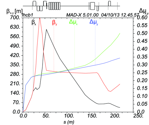
Figure 2: (color online) The horizontal $\beta_{x}$ and vertical betatron amplitude $\beta_{y}$ for the LHC $\beta^{*}=3.5$ m optics. The horizontal $\Delta\mu_{x}$ and vertical phase advance $\Delta\mu_{y}$ are also shown, these functions are normalized to $2\pi$. The plot shows that the horizontal phase advance $\Delta\mu_{x}=\pi$ close to the far RP unit.

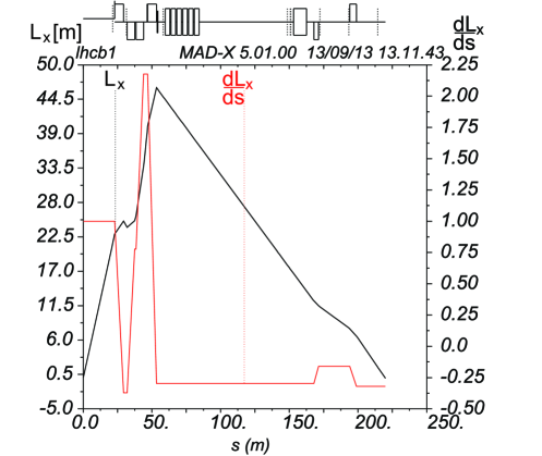
Figure 3: (color online) The horizontal effective length $L_{x}$ and its derivative $\rmd L_{x}/\rmd s$ with respect to $s$ as a function of the distance $s$ in case of the LHC $\beta^{*}=3.5$ m optics. The evolution of the optical functions is shown starting from IP5 up to the Roman Pot stations. The plot indicates that $L_{x}=0$ close to the far RP unit, thus in the reconstruction of proton kinematics, $\rmd L_{x}/\rmd s$ is used instead of $L_{x}$ .

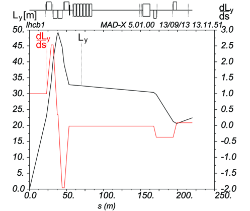
Figure 4: (color online) The evolution of the vertical effective length $L_{y}$ and its derivative $\rmd L_{y}/\rmd s$ between IP5 and the location of the Roman Pot stations, for the $\beta^{*}=3.5$ m optics of the LHC.

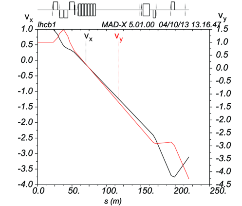
Figure 5: (color online) The evolution of the horizontal $\nu_{x}$ and vertical $\nu_{y}$ magnifications, for the $\beta^{*}=3.5$ m optics of the LHC.

In summary, the kinematics of elastically scattered protons at IP5 can be reconstructed on the basis of RP proton tracks using (1):

$$\Theta_{y}^{*}\approx\frac{y}{L_{y}}\,,\,\qquad\Theta_{x}^{*}\approx\frac{1}{\frac{\rmd L_{x}}{\rmd s}}\left(\Theta_{x}-\frac{\rmd v_{x}}{\rmd s}x^{*}\right)\,,\,\qquad x^{*}=\frac{x}{v_{x}}\,.$$ (12)

The vertical effective length $L_{y}$ and the horizontal magnification $v_{x}$ are applied in (12) due to their sizeable values, as shown in figures 4 and 5. As the values of the reconstructed angles are inversely proportional to the optical functions, the errors of the optical functions dominate the systematic errors of the final, physics results of TOTEM RP measurements.

The proton transport matrix $T\left(s;\mathcal{M}\right)$, calculated with MAD-X [14], is defined by the machine settings $\mathcal{M}$, which are obtained on the basis of several data sources: the magnet currents are first retrieved from TIMBER [15] and then converted to magnet strengths with LSA [16], implementing the conversion curves measured by FIDEL [17]. The WISE database [18] contains the measured imperfections (field harmonics, magnet displacements and rotations) included in $\mathcal{M}$.

3 Machine imperfections

The real LHC machine [2] is subject to additional imperfections $\Delta\mathcal{M}$, not measured well enough so far, which alter the transport matrix by $\Delta T$:

$$T\left.(s;\,\mathcal{M}\right)\rightarrow T\left.(s;\,\mathcal{M}+\Delta\mathcal{M}\right)=T\left.(s;\,\mathcal{M}\right)+\Delta T.$$ (13)

The most important transport matrix imperfections are due to:

• the magnet current–strength conversion error: $\sigma(k)/k\approx 10^{-3}$,

• the beam momentum offset: $\sigma(p)/p\approx 10^{-3}\,$.

Their impact on the important optical functions $L_{y}$ and $\rmd L_{x}/\rmd s$ is presented in table 1. It is clearly visible that the imperfections of the inner triplet (the so called MQXA and MQXB magnets) are of high influence on the transport matrix while the optics is less sensitive to the strength of the quadrupoles MQY and MQML.

Other imperfections that are of lower, but not negligible, significance:

• magnet rotations: $\delta\phi\approx 1$ mrad,

• beam harmonics: $\delta B/B\approx 10^{-4}$,

• power converter errors: $\delta I/I\approx 10^{-4}$,

• magnet positions: $\delta x,\delta y\approx 100\,\mu$m.

Generally, as indicated in table 1, for high-$\beta^{*}$ optics the magnitude of $\Delta T$ is sufficiently small from the viewpoint of data analysis.

However, the sensitivity of the low-$\beta^{*}$ optics to the machine imperfections is significant and cannot be neglected.

	${\delta L_{y,b_{1},far}/L_{y,b_{1},far}}$ [%]		$\delta\left(\frac{\rmd L_{x,b_{1}}}{\rmd s}\right)/\frac{\rmd L_{x,b_{1}}}{\rmd s}$ [%]
Perturbed element	${\beta^{*}=3.5\,m}$	${\beta^{*}=90\,m}$	${\beta^{*}=3.5\,m}$	${\beta^{*}=90\,m}$
MQXA.1R5	$\phantom{-}0.98$	$\phantom{-}0.14$	$-0.46$	$-0.42$
MQXB.A2R5	$-2.24$	$-0.23$	$\phantom{-}0.33$	$\phantom{-}0.31$
MQXB.B2R5	$-2.42$	$-0.25$	$\phantom{-}0.45$	$\phantom{-}0.42$
MQXA.3R5	$\phantom{-}1.45$	$\phantom{-}0.20$	$-1.14$	$-1.08$
MQY.4R5.B1	$-0.10$	$-0.01$	$-0.02$	$\phantom{-}0.00$
MQML.5R5.B1	$\phantom{-}0.05$	$\phantom{-}0.04$	$\phantom{-}0.05$	$\phantom{-}0.06$
$\Delta$p${}_{b_{1}}$/p${}_{b_{1}}$	$-2.19$	$\phantom{-}0.01$	$-0.79$	$\phantom{-}0.71$
Total sensitivity	$\phantom{-}4.33$	$\phantom{-}0.42$	$\phantom{-}1.57$	$\phantom{-}1.46$

Table 1: Sensitivity of the vertical effective length $L_{y,b_{1}}$ and $\rmd L_{x,b_{1}}/\rmd s$ to 1 $\permil$ deviations of magnet strengths or beam momentum for low- and high-$\beta^{*}$ optics of the LHC beam 1. The subscript $b_{1}$ indicates Beam 1. Only the most important contributions are presented.

The proton reconstruction is based on (12). Thus it is necessary to know the effective lengths $L_{x,y}$ and their derivatives with an uncertainty better than $1$–$2\,\%$ in order to measure the total cross-section $\sigma_{\rm tot}$ with the aimed uncertainty of [19]. The currently available $\Delta\beta/\beta$ beating measurement with an error of $5-10$ % does not allow to estimate $\Delta T$ with the uncertainty, required by the TOTEM physics program [20]. However, as it is shown in the following sections, $\Delta T$ can be determined well enough from the proton tracks in the Roman Pots, by exploiting the properties of the optics and those of the elastic $pp$ scattering, so that the aimed 1% relative uncertainty in the determination of the total pp cross-section becomes within the reach of TOTEM.

4 Correlations in the transport matrix

The transport matrix $T$ defining the proton transport from IP5 to the RPs is a product of matrices that describe the magnetic field of the lattice elements along the proton trajectory. The imperfections of the individual magnets alter the cumulative transport function. It turns out that independently of the origin of the imperfection (strength of any of the magnets, beam momentum offset) the transport matrix is altered in a similar way, as can be described quantitatively with eigenvector decomposition, discussed in section 4.1.

4.1 Correlation matrix of imperfections

Assuming that the imperfections discussed in section 2 are independent, the covariance matrix describing the relations among the errors of the optical functions can be calculated:

$$V=\mathrm{Cov}(\Delta T_{r})={E}\left(\Delta T_{r}\Delta T_{r}^{{T}}\right),$$ (14)

where $T_{r}$ is the relevant 8-dimensional subset of the transport matrix

$$T_{r}^{\mbox{\rm\small T}}=(v_{x},L_{x},\frac{\rmd v_{x}}{\rmd s},\frac{\rmd L_{x}}{\rmd s},v_{y},L_{y},\frac{\rmd v_{y}}{\rmd s},\frac{\rmd L_{y}}{\rmd s})\,,$$ (15)

which is presented as a vector for simplicity.

The optical functions contained in $T_{r}$ differ by orders of magnitude and, are expressed in different physical units. Therefore, a normalization of $V$ is necessary and the use of the correlation matrix $C$, defined as

$$C_{i,j}=\frac{V_{i,j}}{\sqrt{V_{i,i}\cdot V_{j,j}}}\,,$$ (16)

is preferred. An identical behaviour of uncertainties for both beams was observed and therefore it is enough to study the Beam 1. In case of the $\beta^{*}=3.5\,$m optics the following error correlation matrix is obtained:

$$C = {\left(\begin{array}[]{cccccccc}\phantom{-}1.00&\phantom{-}0.74&-0.42&-0.80&-0.51&-0.46&-0.61&-0.44\\ \phantom{-}0.74&\phantom{-}1.00&-0.63&-1.00&-0.25&-0.30&-0.32&-0.29\\ -0.42&-0.63&\phantom{-}1.00&\phantom{-}0.62&\phantom{-}0.03&\phantom{-}0.07&\phantom{-}0.01&\phantom{-}0.08\\ -0.80&-1.00&\phantom{-}0.62&\phantom{-}1.00&\phantom{-}0.29&\phantom{-}0.33&\phantom{-}0.37&\phantom{-}0.32\\ -0.51&-0.25&\phantom{-}0.03&\phantom{-}0.29&\phantom{-}1.00&\phantom{-}0.99&\phantom{-}0.98&\phantom{-}0.98\\ -0.46&-0.30&\phantom{-}0.07&\phantom{-}0.33&\phantom{-}0.99&\phantom{-}1.00&\phantom{-}0.96&\phantom{-}1.00\\ -0.61&-0.32&\phantom{-}0.01&\phantom{-}0.37&\phantom{-}0.98&\phantom{-}0.96&\phantom{-}1.00&\phantom{-}0.95\\ -0.44&-0.29&\phantom{-}0.08&\phantom{-}0.32&\phantom{-}0.98&\phantom{-}1.00&\phantom{-}0.95&\phantom{-}1.00\\ \end{array}\right)}\,.$$ (25)

The non-diagonal elements of $C$, which are close to $\pm 1$, indicate strong correlations between the elements of $\Delta T_{r}$. Consequently, the machine imperfections alter correlated groups of optical functions.

This observation can be further quantified by the eigenvector decomposition of $C$, which yields the following vector of eigenvalues $\lambda(C)$ for the $\beta^{*}=3.5\,$m optics:

$$\lambda(C)=\left(4.9,\,2.3,\,0.53,\,0.27,\,0.01,\,0.01,\,0.00,\,0.00\right).$$ (26)

Since the two largest eigenvalues $\lambda_{1}=4.9$ and $\lambda_{2}=2.3$ dominate the others, the correlation system is practically two dimensional with the following two eigenvectors

$$v_{1} =\left(\phantom{-}0.35,\,\phantom{-}0.30,\,-0.16,\,-0.31,\,-0.40,\,-0.41,\,-0.41,\,-0.40\right)\,,$$ (27)

$$v_{2} =\left(-0.26,\,-0.46,\,\phantom{-}0.47,\,\phantom{-}0.45,\,-0.29,\,-0.27,\,-0.25,\,-0.28\right)\,.$$ (28)

Therefore, contributions of the individual lattice imperfections cannot be evaluated. On the other hand, as the imperfections alter approximately only a two-dimensional subspace, a measurement of a small set of weakly correlated optical functions would theoretically yield an approximate knowledge of $\Delta T_{r}$.

4.2 Error estimation of the method

Let us assume for the moment that we can precisely reconstruct the contributions to $\Delta T_{r}$ of the two most significant eigenvectors while neglecting that of the others. The error of such reconstructed transport matrix can be estimated by evaluating the contribution of the remaining eigenvectors:

$$\delta\Delta T_{r,i}=\sqrt{E_{i,i}\cdot V_{i,i}}\,,$$ (29)

where

$$E=N\cdot\left(\begin{array}[]{ccccc}0&0&0&0&0\\ 0&0&0&0&0\\ 0&0&\lambda_{3}&0&0\\ \vdots&&&\ddots&\vdots\\ 0&0&0&0&\lambda_{8}\\ \end{array}\right)\cdot N^{\mathrm{T}}$$ (30)

and $N=\left(\nu_{1},...,\nu_{8}\right)$ is the basis change matrix composed of eigenvectors $\nu_{i}$ corresponding to the eigenvalues $\lambda_{i}$.

The relative optics uncertainty before and after the estimation of the most significant eigenvectors is summarized in table 2.

	$v_{x,far}$	$L_{x,far}$	$\frac{\rmd v_{x}}{\rmd s}$	$\frac{\rmd L_{x}}{\rmd s}$
$T_{r,i}$	$-3.1$	$-1.32\cdot 10^{-1}$ m	$\phantom{-}3.1\cdot 10^{-2}$ m-1	$-3.21\cdot 10^{-1}$
$\frac{\sqrt{V_{i,i}}}{\left|T_{r,i}\right|}$ [%]	$2.0\cdot 10^{-1}$	$3.4\cdot 10^{2}$	$4.2\cdot 10^{-1}$	$1.6$
$\frac{\delta\Delta T_{r,i}}{\left|T_{r,i}\right|}$ [%]	$9.5\cdot 10^{-2}$	$9.1\cdot 10^{1}$	$2.6\cdot 10^{-1}$	$3.4\cdot 10^{-1}$

	$v_{y,far}$	$L_{y,far}$	$\frac{\rmd v_{y}}{\rmd s}$	$\frac{\rmd Ly}{\rmd s}$
$T_{r,i}$	$-4.3$	$\phantom{-}2.24\cdot 10^{1\phantom{-}}$ m	$-6.1\cdot 10^{-2}$ m-1	$\phantom{-}8.60\cdot 10^{-2}$
$\frac{\sqrt{V_{i,i}}}{\left|T_{r,i}\right|}$ [%]	$6.8\cdot 10^{-1}$	$4.3$	$5.9\cdot 10^{-1}$	$1.5\cdot 10^{1}$
$\frac{\delta\Delta T_{r,i}}{\left|T_{r,i}\right|}$ [%]	$6.1\cdot 10^{-2}$	$6.4\cdot 10^{-1}$	$8.3\cdot 10^{-2}$	$2.75$

Table 2: Nominal values of the optical functions $T_{r,i}$ and their relative uncertainty before ($\sqrt{V_{i,i}}/\left|T_{r,i}\right|$) and after ($\delta\Delta T_{r,i}/\left|T_{r,i}\right|$) the determination of the two most significant eigenvectors ($\beta^{*}=3.5\,$m, Beam 1).

According to the table, even if we limit ourselves only to the first two most significant eigenvalues, the uncertainty of optical functions due to machine imperfections drops significantly. In particular, in case of $\rmd L_{x}/\rmd s$ and $L_{y}$ a significant error reduction down to a per mil level is observed. Unfortunately, due to $\Delta\mu_{x}=\pi$ (figure 2), the uncertainty of $L_{x}$, although importantly improved, remains very large and the use of $\rmd L_{x}/\rmd s$ for proton kinematics reconstruction should be preferred.

In the following sections a practical numerical method of inferring the optics from the RP proton tracks is presented and its validation with Monte Carlo calculations is reported.

5 Optics estimators from proton tracks measured by Roman Pots ($\boldsymbol{\beta}^{*}$=3.5 m optics)

The TOTEM experiment can select the elastically scattered protons with high purity and efficiency [8, 9]. The RP detector system, due to its high resolution ($\sigma(x,y)\approx 11\,\mu$m, $\sigma(\Theta_{x,y})\approx 2.9\,\mu$rad), can measure very precisely the proton angles, positions and the angle-position relations on an event-by-event basis. These quantities can be used to define a set of estimators characterizing the correlations between the elements of the transport matrix $T$ or between the transport matrices of the two LHC beams. Such a set of estimators $\hat{R}_{1},...,\hat{R}_{10}$ (defined in the next sections) is exploited to reconstruct, for both LHC beams, the imperfect transport matrix $T(\mathcal{M})+\Delta T$ defined in (13).

5.1 Correlations between the beams

Since the momentum of the two LHC beams is identical, the elastically scattered protons will be deflected symmetrically from their nominal trajectories of Beam 1 and Beam 2:

$$\Theta^{*}_{x,b_{1}}=-\Theta^{*}_{x,b_{2}}\,,\Theta^{*}_{y,b_{1}}=-\Theta^{*}_{y,b_{2}}\,,$$ (31)

which allows to compute ratios $R_{1,2}$ relating the effective lengths at the RP locations of the two beams. From (1) and (31) we obtain:

$$R_{1} \equiv\frac{\Theta_{x,b_{1}}}{\Theta_{x,b_{2}}}\approx\frac{\frac{\rmd L_{x,b_{1}}}{\rmd s}\cdot\Theta^{*}_{x,b_{1}}}{\frac{\rmd L_{x,b_{2}}}{\rmd s}\cdot\Theta^{*}_{x,b_{2}}}=-\frac{\frac{\rmd L_{x,b_{1}}}{\rmd s}}{\frac{\rmd L_{x,b_{2}}}{\rmd s}}\,,$$ (32)

$$R_{2} \equiv\frac{y_{b_{1},far}}{y_{b_{2},far}}\approx-\frac{L_{y,b_{1},far}}{L_{y,b_{2},far}}\,,$$ (33)

where the subscripts $b_{1}$ and $b_{2}$ indicate Beam 1 and 2, respectively. Approximations present in (32) and (33) represent the impact of statistical effects such as detector resolution, beam divergence and primary vertex position distribution. The estimators $\hat{R}_{1}$ and $\hat{R}_{2}$ are finally obtained from the $(\Theta_{x,b_{1}},\Theta_{x,b_{2}})$ and $(y_{b_{1},far},y_{b_{2},far})$ distributions and are defined with the help of the distributions’ principal eigenvector, as illustrated in figures 6 and 7.

The width of the distributions is determined by the beam divergence and the vertex contribution, which leads to 0.5% uncertainty on the eigenvector’s slope parameter.

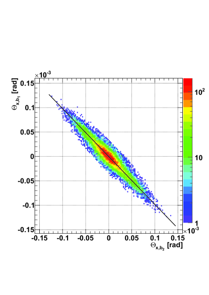
Figure 6: (color online) Beam 1 and 2 elastic scattering angle correlation in the horizontal plane $(\Theta_{x,b_{1}},\Theta_{x,b_{2}})$ of protons detected by the Roman Pots.

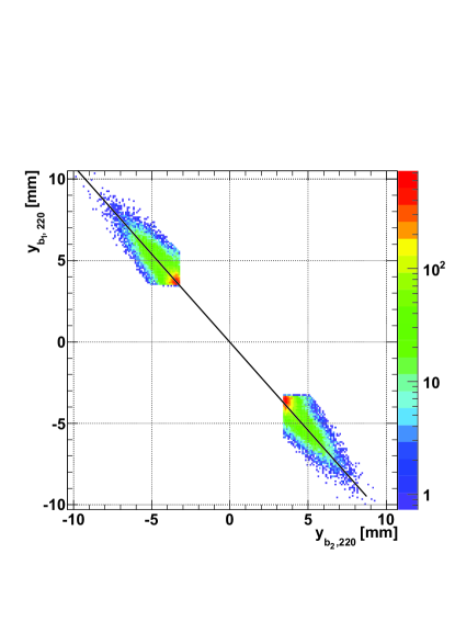
Figure 7: (color online) Correlation between positions (vertical projections) of elastically scattered protons detected in Beam 1 and 2. The sharp edges are due to the vertical acceptance limits of the detectors.

5.2 Single beam correlations

The distributions of proton angles and positions measured by the Roman Pots define the ratios of certain elements of the transport matrix $T$, defined by (1) and (7). First of all, $\rmd L_{y}/\rmd s$ and $L_{y}$ are related by

$$R_{3}\equiv\frac{\Theta_{y,b_{1}}}{y_{b_{1}}}\approx\frac{\frac{\rmd L_{y,b_{1}}}{\rmd s}}{L_{y,b_{1}}}\,,\;\qquad\quad R_{4}\equiv\frac{\Theta_{y,b_{2}}}{y_{b_{2}}}\approx\frac{\frac{\rmd L_{y,b_{2}}}{\rmd s}}{L_{y,b_{2}}}\,.$$ (34)

The corresponding estimators $\hat{R}_{3}$ and $\hat{R}_{4}$ can be calculated with an uncertainty of 0.5% from the distributions as presented in figure 8.

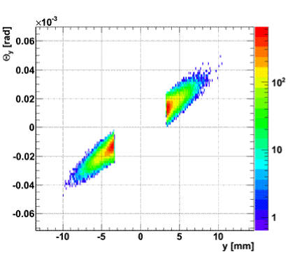
Figure 8: (color online) Correlation between vertical position and angle of elastically scattered protons at the RP of Beam 1.

Similarly, we exploit the horizontal dependencies to quantify the relations between $\rmd L_{x}/\rmd s$ and $L_{x}$. As $L_{x}$ is close to $0$, see figure 3, instead of defining the ratio we rather estimate the position $s_{0}$ along the beam line (with the uncertainty of about $1\,$m), for which $L_{x}=0$. This is accomplished by resolving

$$\frac{L_{x}(s_{0})}{\rmd L_{x}(s_{1})/\rmd s}=\frac{L_{x}(s_{1})}{\rmd L_{x}(s_{1})/\rmd s}+\left(s_{0}-s_{1}\right)=0\,,$$ (35)

for $s_{0}$, where $s_{1}$ denotes the coordinate of the Roman Pot station along the beam with respect to IP5. Obviously, $\rmd L_{x}(s)/\rmd s$ is constant along the RP station as no magnetic fields are present at the RP location. The ratios $L_{x}(s_{1})/\frac{\rmd L_{x}(s_{1})}{\rmd s}$ for Beam 1 and 2, similarly to the vertical constraints $R_{3}$ and $R_{4}$, are defined by the proton tracks:

$$\frac{L_{x}}{\frac{\rmd L_{x}}{\rmd s}}\approx\frac{x}{\Theta_{x}}\,,$$ (36)

which is illustrated in figure 9. In this way two further constraints and the corresponding estimators (for Beam 1 and 2) are obtained:

$$R_{5}\equiv s_{b_{1}}\mathrm{\,\,and\,\,}R_{6}\equiv s_{b_{2}}\,.$$ (37)

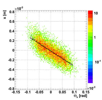
Figure 9: (color online) Correlation between the horizontal angle and position of elastically scattered protons at the RP of Beam 1.

5.3 Coupling / rotation

In reality the coupling coefficients $m_{13},...,m_{42}$ cannot be always neglected, as it is assumed by (11). RP proton tracks can help to determine the coupling components of the transport matrix $T$ as well, where it is especially important that $L_{x}$ is close to zero at the RP locations. Always based on (1) and (7), four additional constraints (for each of the two LHC beams and for each unit of the RP station) can be defined:

$$R_{7,...,10}\equiv\frac{x_{{near(far)}}}{y_{{near(far)}}}\approx\frac{m_{14,{near(far)}}}{L_{y,{near(far)}}}\,.$$ (38)

The subscripts “near” and “far” indicate the position of the RP along the beam with respect to the IP. Geometrically $R_{7,...,10}$ describe the rotation of the RP scoring plane about the beam axis. Analogously to the previous sections, the estimators $\hat{R}_{7,...,10}$ are obtained from track distributions as presented in figure 10 and an uncertainty of $3\%$ is achieved.

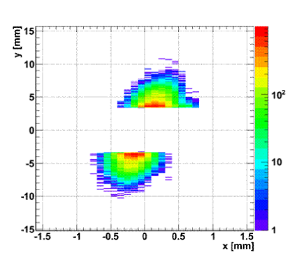
Figure 10: (color online) Vertical vs. horizontal track position at the RP_near of the LHC Beam 1.

6 Optical functions estimation

The machine imperfections $\Delta\mathcal{M}$, leading to the transport matrix change $\Delta T$, are in practice determined with the $\chi^{2}$ minimization procedure:

$$\widehat{\Delta\mathcal{M}}=arg\,min(\chi^{2})\,,$$ (39)

defined on the basis of the estimators $\hat{R}_{1}...\hat{R}_{10}\,$, where the $arg\,min$ function gives the phase space position where the $\chi^{2}$ is minimized. As it was discussed in section 4.1, although the overall alteration of the transport matrix $\Delta T$ can be determined precisely based on a few optical functions’ measurements, the contributions of individual imperfections cannot be established. In terms of optimization, such a problem has no unique solution and additional constraints, defined by the machine tolerance, have to be added.

Therefore, the $\chi^{2}$ function is composed of the part defined by the Roman Pot tracks’ distributions and the one reflecting the LHC tolerances:

$$\chi^{2}=\chi_{Design}^{2}+\chi_{Measured}^{2}\,.$$ (40)

The design part

$$\chi_{Design}^{2}=\sum_{i=1}^{12}\left(\frac{k_{i}-k_{i,{\mbox{\tiny MAD-X}}}}{\sigma(k_{i})}\right)^{2}+\sum_{i=1}^{12}\left(\frac{\phi_{i}-\phi_{i,{\mbox{\tiny MAD-X}}}}{\sigma(\phi_{i})}\right)^{2}+\sum_{i=1}^{2}\left(\frac{p_{i}-p_{i,{\mbox{\tiny MAD-X}}}}{\sigma(p_{i})}\right)^{2}\,$$ (41)

where $k_{i}$ and $\phi_{i}$ are the nominal strength and rotation of the $i$th magnet, respectively. Thus (41) defines the nominal machine $(k_{i},\,\phi_{i},\,p_{i})$ as an attractor in the phase space. Both LHC beams are treated simultaneously. Only the relevant subset of machine imperfections $\Delta\mathcal{M}$ was selected. The obtained 26-dimensional optimization phase space includes the magnet strengths (12 variables), rotations (12 variables) and beam momentum offsets (2 variables). Magnet rotations are included into the phase space, otherwise only the coupling coefficients $m_{13},...,m_{42}$ could induce rotations in the $(x,y)$ plane (38), which could bias the result.

The measured part

$$\chi^{2}_{Measured}=\sum_{i=1}^{10}\left(\frac{\hat{R}_{i}-R_{i,{\mbox{\tiny MAD-X}}}}{\sigma(\hat{R}_{i})}\right)^{2}$$ (42)

contains the track-based estimators $\hat{R}_{1}...\hat{R}_{10}$ (discussed in detail in section 5) together with their uncertainty. The subscript “MAD-X” defines the corresponding values evaluated with the MAD-X software during the $\chi^{2}$ minimization.

Table 3 presents the results of the optimization procedure for the $\beta^{*}=3.5\,$m optics used by LHC in October 2010 at beam energy $E=3.5\,$TeV.

The obtained value of the effective length $L_{y}$ of Beam 1 is close to the nominal one, while Beam 2 shows a significant change. The same pattern applies to the values of $\rmd L_{x}/\rmd s$. The error estimation of the procedure is discussed in section 7.

	${L_{y,b_{1},far}}$[m]	${\rmd L_{x,b_{1}}/\rmd s}$	${L_{y,b_{2},far}}$[m]	${\rmd L_{x,b_{2}}/\rmd s}$
Nominal	$22.4$	$-3.21\cdot 10^{-1}$	$18.4$	$-3.29\cdot 10^{-1}$
Estimated	$22.6$	$-3.12\cdot 10^{-1}$	$20.7$	$-3.15\cdot 10^{-1}$

Table 3: Selected optical functions of both LHC beams for the $\beta^{*}=3.5\,$m optics, obtained with the estimation procedure, compared to their nominal values.

7 Monte Carlo validation

In order to demonstrate that the proposed $\hat{R}_{i}$ optics estimators are effective the method was validated with Monte Carlo simulations.

In each Monte Carlo simulation the nominal machine settings $\mathcal{M}$ were altered with simulated machine imperfections $\Delta\mathcal{M}$ within their tolerances using Gaussian distributions. The simulated elastic proton tracks were used afterwards to calculate the estimators $\hat{R}_{1}...\hat{R}_{10}$. The study included the impact of

• magnet strengths,

• beam momenta,

• magnet displacements, rotations and harmonics,

• settings of kickers,

• measured proton angular distribution.

The error distributions of the optical functions $\Delta T$ obtained for $\beta^{*}=3.5\,$m and $E=3.5\,$TeV are presented in figure 11 and table 4, while the $\beta^{*}=90\,$m results at $E=4\,$TeV are shown in figure 12 and table 5.

	Simulated		Reconstructed
	optics distribution		optics error
Relative optics	Mean	RMS	Mean	RMS
distribution	[%]	[%]	[%]	[%]
$\frac{\delta L_{y,b_{1},far}}{L_{y,b_{1},far}}\;$	$\phantom{-}0.39$	$4.2$	$\phantom{-}8.3\cdot 10^{-2}$	$0.16$
$\frac{\delta\rmd L_{x,b_{1}}/\rmd s}{\rmd L_{x,b_{1}}/\rmd s}\;$	$-0.97$	$1.6$	$-0.13$	$0.17$
$\frac{\delta L_{y,b_{2},far}}{L_{y,b_{2},far}}\;$	$-0.14$	$4.9$	$\phantom{-}0.21$	$0.16$
$\frac{\delta\rmd L_{x,b_{2}}/\rmd s}{\rmd L_{x,b_{2}}/\rmd s}\;$	$\phantom{-}0.10$	$1.7$	$-9.7\cdot 10^{-2}$	$0.17$

Table 4: The Monte-Carlo study of the impact of the LHC imperfections $\Delta\mathcal{M}$ on selected transport matrix elements $\rmd L_{x}/\rmd s$ and $L_{y}$ for $\beta^{*}=3.5\,$m at $E=3.5$ TeV. The LHC parameters were altered within their tolerances. The relative errors of $\rmd L_{x}/\rmd s$ and $L_{y}$ (mean value and RMS) characterize the optics uncertainty before and after optics estimation.

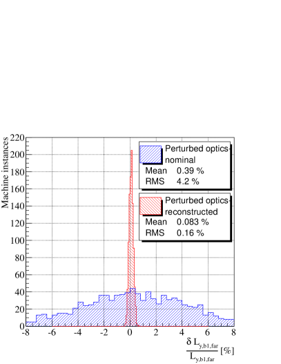
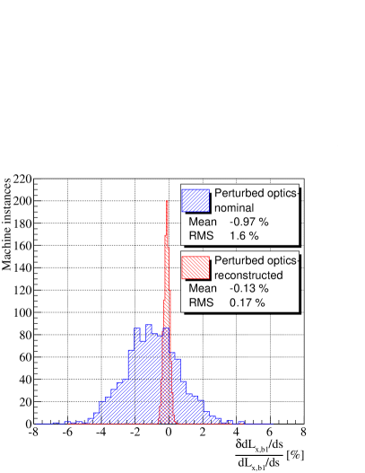
Figure 11: (color online) The MC error distribution of $\beta^{*}=3.5$ m optical functions $L_{y}$ and $\rmd L_{x}/\rmd s$ for Beam 1 at $E=3.5$ TeV, before and after optics estimation.

	Simulated		Reconstructed
	optics distribution		optics error
Relative optics	Mean	RMS	Mean	RMS
distribution	[%]	[%]	[%]	[%]
$\frac{\delta L_{y,b_{1},far}}{L_{y,b_{1},far}}\;$	$2.2\cdot 10^{-2}$	$0.46$	$\phantom{-}5.8\cdot 10^{-2}$	$0.23$
$\frac{\delta\rmd L_{x,b_{1}}/\rmd s}{\rmd L_{x,b_{1}}/\rmd s}\;$	$6.7\cdot 10^{-3}$	$1.5$	$-6.4\cdot 10^{-2}$	$0.20$
$\frac{\delta L_{y,b_{2},far}}{L_{y,b_{2},far}}\;$	$-5\cdot 10^{-3}$	$0.47$	$5.8\cdot 10^{-2}$	$0.23$
$\frac{\delta\rmd L_{x,b_{2}}/\rmd s}{\rmd L_{x,b_{2}}/\rmd s}\;$	$1.8\cdot 10^{-2}$	$1.5$	$-7\cdot 10^{-2}$	$0.21$

Table 5: The Monte-Carlo study of the impact of the LHC imperfections $\Delta\mathcal{M}$ on selected transport matrix elements $\rmd L_{x}/\rmd s$ and $L_{y}$ for $\beta^{*}=90\,$m at $E=4$ TeV. The LHC parameters were altered within their tolerances. The relative errors of $\rmd L_{x}/\rmd s$ and $L_{y}$ (mean value and RMS) characterize the optics uncertainty before and after optics estimation.

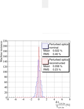
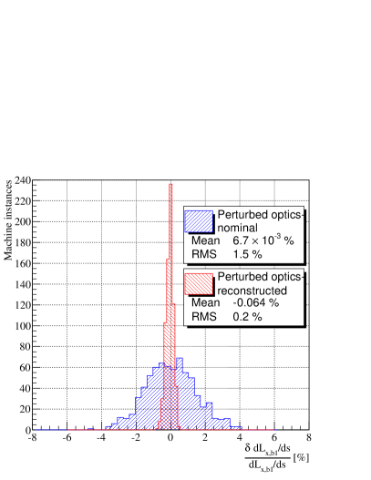
Figure 12: (color online) The MC error distribution of $\beta^{*}=90$ m optical functions $L_{y}$ and $\rmd L_{x}/\rmd s$ for Beam 1 at $E=4$ TeV, before and after optics estimation.

First of all, the impact of the machine imperfections $\Delta\mathcal{M}$ on the transport matrix $\Delta T$, as shown by the MC study, is identical to the theoretical prediction presented in table 2. The bias of the simulated optics distributions is due to magnetic field harmonics as reported by the LHC imperfections database [18]. The final value of mean after optics estimation procedure contributes to the total uncertainty of the method.

The errors of the reconstructed optical functions are significantly smaller than evaluated theoretically in section 4.2. This results from the larger number of design and measured constraints (40), employed in the numerical estimation procedure of section 6. In particular, the collinearity of elastically scattered protons was exploited in addition. Finally, the achieved uncertainties of $\rmd L_{x}/\rmd s$ and $L_{y}$ are both lower than $2.5\,\permil$ for both beams.

8 Conclusions

TOTEM has proposed a novel approach to estimate the optics at LHC. The method, based on the correlations of the transport matrix, consists of the determination of the optical functions, which are strongly correlated to measurable combinations of the transport matrix elements.

At low-$\beta^{*}$ LHC optics, where machine imperfections are more significant, the method allowed us to determine the real optics with a per mil level uncertainty, and also permitted to assess the errors of the transport matrix errors from the tolerances of various machine parameters. In case of high-$\beta^{*}$ LHC optics, where the machine imperfections have smaller effect on the optical functions, the method remains effective and reduces the uncertainties to the desired per mil level. The method has been validated with the Monte Carlo studies both for high- and low-$\beta^{*}$ optics and was successfully used in the TOTEM experiment to calibrate the optics of the LHC accelerator directly from data in physics runs for precision TOTEM measurements of the total pp cross-section.

References

References

- [1] Antchev G et al. 2008 JINST 3 S08007
- [2] Evans L and Bryant P 2008 JINST 3 S08001
- [3] Anelli G et al. 2008 JINST 3 S08007
- [4] Antchev G et al. 2013 Int. J. Mod. Phys. A 28 1330046
- [5] Kašpar J 2011 PhD Thesis CERN-THESIS-2011-214
- [6] Burkhardt H and White S 2010 “High- Optics for the LHC” LHC Project Note 431
- [7] Niewiadomski H 2008 PhD Thesis CERN-THESIS-2008-080
- [8] Antchev G et al. 2011 Europhys. Lett. 95 41001
- [9] Antchev G et al. 2011 Europhys. Lett. 96 21002
- [10] Antchev G et al. 2013 Europhys. Lett. 101 21002
- [11] Antchev G et al. 2013 Europhys. Lett. 101 21004
- [12] Antchev G et al. 2013 Phys. Rev. Lett. 111 012001
- [13] Wiedemann H 2007 Particle Accelerator Physics, 3rd ed., ISBN: 978-3540490432, Springer
- [14] MAD-X : An Upgrade from MAD8, CERN-AB-2003-024-ABP.
- [15] The LHC Logging Service, CERN-AB-Note-2006-046.
- [16] The LSA Database to Drive the Accelerator Settings, CERN-ATS-2009-100.
- [17] FIDEL – The Field Description for the LHC, LHC-C-ES-0012 ver.2.0.
- [18] WISE: A Simulation of the LHC Optics Including Magnet Geometrical Data, Proc. of EPAC08, Genova, Italy.
- [19] Berardi V et al. 2004 TOTEM Technical Design Report. 1st ed. CERN, Geneva, ISBN 9290832193.
- [20] Tomás R et al. 2010 LHC Optics Model Measurements and Corrections, Proc. of IPAC10, Kyoto, Japan