How does pressure gravitate?
Cosmological constant problem confronts observational cosmology

Abstract

An important and long-standing puzzle in the history of modern physics is the gross inconsistency between theoretical expectations and cosmological observations of the vacuum energy density, by at least 60 orders of magnitude, otherwise known as the cosmological constant problem. A characteristic feature of vacuum energy is that it has a pressure with the same amplitude, but opposite sign to its energy density, while all the precision tests of General Relativity are either in vacuum, or for media with negligible pressure. Therefore, one may wonder whether an anomalous coupling to pressure might be responsible for decoupling vacuum from gravity. We test this possibility in the context of the Gravitational Aether proposal, using current cosmological observations, which probe the gravity of relativistic pressure in the radiation era. Interestingly, we find that the best fit for anomalous pressure coupling is about half-way between General Relativity (GR), and Gravitational Aether (GA), if we include Planck together with WMAP and BICEP2 polarization cosmic microwave background (CMB) observations. Taken at face value, this data combination excludes both GR and GA at around the $3\,\sigma$ level. However, including higher resolution CMB observations (“highL”) or baryonic acoustic oscillations (BAO) pushes the best fit closer to GR, excluding the Gravitational Aether solution to the cosmological constant problem at the 4–$5\,\sigma$ level. This constraint effectively places a limit on the anomalous coupling to pressure in the parametrized post-Newtonian (PPN) expansion, $\zeta_{4}=0.105\pm 0.049$ (+highL CMB), or $\zeta_{4}=0.066\pm 0.039$ (+BAO). These represent the most precise measurement of this parameter to date, indicating a mild tension with GR (for $\Lambda$CDM including tensors, with $\zeta_{4}=0$), and also among different data sets.

I Introduction

One of the most immediate puzzles of quantum gravity (i.e., applying the rules of quantum mechanics to gravitational physics) is an expectation value for the vacuum energy that is 60–120 orders of magnitude larger than its measured value from cosmological (gravitational) observations. This is known as the (now old) cosmological constant problem Weinberg (1989), and has been thwarting our understanding of modern physics for almost a century Straumann (2003). The discovery of late-time cosmic acceleration Riess et al. (1998); Perlmutter et al. (1999), added an extra layer of complexity to the puzzle, showing that the (gravitational) vacuum energy, albeit tiny, is non-vanishing (now dubbed, the new cosmological constant problem).

Gravitational Aether (GA) theory is an attempt to find a solution to the old cosmological constant problem Afshordi (2008); Aslanbeigi et al. (2011), i.e., the question of why, in lieu of fantastic cancellations, the vacuum quantum fluctuations do not appear to source gravity. The approach is to stop the quantum vacuum from gravitating by modifying our theory of gravity, as we describe below. In this way the (mean density of ) quantum fluctuations will have no dynamical effect in astrophysics or cosmology (see Zel’dovich (1968) for one of the very first steps and Thomas et al. (2009) for an alternative but related attempt for solving the problem).

Although GA is a very specific proposal for modifying gravity, it may serve as an example of more general theories. As we will see below, a generalized version may represent a broader class of theories in which the gravitational effects of pressure (and including anisotropic stress) might be different from those of GR.

It is important to be clear that this theory does not have any solution for the “new” cosmological constant problem, i.e., the empirical existence of a small vacuum energy density which now dominates the energy budget of the Universe, driving the accelerated expansion and making the geometry of space close to flat. Hence in GA theory it is assumed that the vacuum quantum fluctuations (the old problem) and the small but non-zero value of $\Lambda$ (the new problem) are two separate phenomena that should be explained independently (but see Prescod-Weinstein et al. (2009)).

The Einstein field equations in the GA theory (in units with $c=1$, and with metric signature=(–+++)) are modified to

$$(8\,\pi\,G_{\mbox{\tiny{R}}})^{-1}(G_{\mu\nu}+\Lambda g_{\mu\nu}) = T_{\mu\nu}-\dfrac{1}{4}T^{\alpha}_{\alpha}g_{\mu\nu}+T^{\prime}_{\mu\nu},$$ (1)

$${\rm with}\ T^{\prime}_{\mu\nu} = p^{\prime}(u^{\prime}_{\mu}u^{\prime}_{\nu}+g_{\mu\nu}).$$ (2)

Most significantly, the second term on the right hand side of Eq. 1, $-\frac{1}{4}T^{\alpha}_{\alpha}g_{\mu\nu}$, solves the old cosmological constant problem by cancelling the effect of vacuum fluctuations in the energy momentum tensor. The third term, $T^{\prime}_{\mu\nu},$ is then needed to make the field equations consistent, and is dubbed gravitational aether.

The form used for $T^{\prime}_{\mu\nu}$ in Eq. 2 is a convenient choice, but is probably not unique, although it is limited by phenomenological and stability constraints Afshordi (2008). However, $p^{\prime}$ and $u^{\prime}_{\mu}$, the pressure and four velocity unit vector of the aether, are constrained through the terms in the energy-momentum tensor by applying the Bianchi identity and the assumption of energy-momentum conservation, i.e.,

$$\nabla^{\mu}T^{\prime}_{\mu\nu}=\dfrac{1}{4}\nabla_{\nu}T.$$ (3)

The only free constant of this theory, as in General Relativity (GR), is $G_{\mbox{\tiny{R}}}$, although, as we will see, this is not the same as the usual Newtonian gravitational constant, $G_{\mbox{\tiny{N}}}$. In addition, of course, there are parameters describing the constituents in the various tensors, i.e., the cosmological parameters. In cosmology, the energy-momentum tensor, $T_{\mu\nu}$, consists of the conventional fluids, i.e., radiation, baryons, and cold dark matter, plus a contribution due to vacuum fluctuations,

$$T_{\mu\nu} = T^{{\rm R}}_{\mu\nu}+T^{{\rm B}}_{\mu\nu}+T^{{\rm C}}_{\mu\nu}+\rho_{\rm vac}g_{\mu\nu},$$ (4)

$$T \equiv T^{\alpha}_{\alpha}\,=\,-(\rho^{\rm B}+\rho^{\rm C})+4\,\rho_{\rm vac},$$ (5)

where neutrinos are included as part of radiation, and their mass is set to zero in this paper.

Equations 1 and 2 that describe GA are drastic modifications of GR with no additional tunable parameter. Therefore, one may wonder whether GA can survive all the precision tests of gravity that have already been carried out. These tests are often expressed in terms of the parameterized post-Newtonian (PPN) modifications of GR, which are expressed in terms of 10 dimensionless PPN parameters Will (2014). While these parameters do not capture all possible modifications of GR, they are usually sufficient to capture leading corrections to GR predictions in the post-Newtonian regime (i.e., nearly flat space-time with non-relativistic motions), in lieu of new scales in the gravitational theory. It turns out that only one PPN parameter, $\zeta_{4}$, which quantifies the anomalous coupling of gravity to pressure has not been significantly constrained empirically, as the existing precision tests only probe gravity in vacuum, or for objects with negligible pressure. Indeed, since only the sourcing of gravity is modified in GA, the vacuum gravity content is identical to GR, and the only PPN parameter that deviates from GR is $\zeta_{4}=1/3$ (as opposed to $\zeta_{4}=0$ in GR) Afshordi (2008); Aslanbeigi et al. (2011).

The idea that $\zeta_{4}$ could be non-zero runs contrary to the conventional wisdom that relates gravitational coupling to pressure on the one hand, to the couplings to internal and kinetic energies on the other Will (1976), both of which are already significantly constrained by experiments. However, this expectation is based on the assumption that the average gravity of a gas of interacting point particles, is the same as the gravity of a perfect fluid that is obtained by coarse-graining the particle gas . This connects with the whole issue of the assumption of the continuum approximation for cosmological fluids, where the particle density is low, so that the average distance between particles is a macroscopic scale. Gravity is only well-tested on scales $\gtrsim 0.1\,$mm Kapner et al. (2007), which are larger than the distance between particles in most terrestrial or astrophysical precision tests of gravity. Therefore, there is no guarantee that the same laws of gravity apply to microscopic constituents of the continuous media in which gravity is currently tested. Indeed, GA could only be an effective theory of gravity above some scale $\lambda_{\rm c}\lesssim 0.1$ mm, implying that sources of energy-momentum on the right hand sides of Eqs. 1 or 3 should be coarse-grained on scale $\lambda_{\rm c}$.

At first sight, it might appear that the dependence of gravitational coupling on pressure signals a violation of weak and/or strong equivalence principles (WEP and/or SEP). However, WEP is explicitly imposed in GA, as all matter components couple to the same metric. Moreover, SEP is so far only tested for gravity in vacuum (e.g. point masses in the solar system), where GA is equivalent to GR, as aether is not sourced, and thus vanishes (in lieu of non-trivial boundary conditions; see e.g. Prescod-Weinstein et al. (2009)).

What goes against one’s intuition in the case of the GA modification of Einstein gravity, compared to e.g. scalar-tensor theories, is that even in the Newtonian limit, comparable effects come from the change in couplings and the gravity of the energy/momentum of the aether. In contrast, the additional fields in the usual modified gravity theories carry little energy/momentum in the Newtonian regime, while they could modify couplings by order unity. If the change in the gravitational mass (due to the dependence of $G$ on the equation of state) is by the same factor as the change in energy/momentum (due to the additional terms on the RHS of Einstein equations), then the ratio of gravitational to inertial mass remains unchanged.

A more intuitive picture might be to consider aether (minus the trace term) as an exotic fluid bound to matter, similar to an electron gas for example, within ordinary GR. Like the electron gas, the effect will be to modify the gravitational field source, by the amount of energy/momentum in the exotic fluid. However, unlike the electron gas, the non-gravitational energy/momentum exchange between matter and the exotic fluid is tuned to zero, which ensures WEP, at least at the classical level. Moreover, the action-reaction principle (Newton’s 3rd law) for gravitational forces should include the momentum in, and interaction with the exotic fluid.

Another conceptual issue with Eqs 1–2 is that, at least to our knowledge, they do not follow from an action principle. However, an action principle may not be necessary (or even possible) for a low energy effective theory, such as in the case of Navier-Stokes fluid equations, even if the fundamental theory does follow from an action principle. Given the severity of the cosmological constant problem, it seems reasonable that we might be prepared to relax requirements that are not absolutely necessary for a sensible effective description of nature.

There are two obvious places in the Universe to look for the gravitational effect of relativistic pressure, and thus constrain $\zeta_{4}$:

1. The first situation involves compact objects, particularly the internal structure of neutron stars Schwab et al. (2008); Kamiab and Afshordi (2011). While, in principle, mass and radius measurements of neutron stars can be used to constrain $\zeta_{4}$, at the moment the constraints are almost completely degenerate with the uncertainty in the nuclear equation of state (not to mention other observational systematics). However, future observations of gravitational wave emission from neutron star mergers (e.g., with Advanced LIGO interferometers) might be able to break this degeneracy Kamiab and Afshordi (2011). It may also be possible to develop tests that probe near the hot accretion disks of black holes or during the formation of compact objects in supernova explosions.

2. The second situation is the matter-radiation transition in the early Universe. Ref. Rappaport et al. (2008) studied constraints arising from the big bang nucleosynthesis epoch. However, more precise measurements come from various cosmic microwave background (CMB) anisotropy experiments, such as the Wilkinson Microwave Anisotropy Probe (WMAP) Hinshaw et al. (2013), Planck Planck Collaboration et al. (2011), the Atacama Cosmology Telescope (ACT) Das et al. (2014), and the South Pole Telescope (SPT) Keisler et al. (2011), amongst other cosmological observations. The constraints on GA were studied in detail in Ref. Aslanbeigi et al. (2011), with the data sets available at that time. While GA might arguably ease tension among certain observations, such as the Ly-$\alpha$ forest, primordial Lithium abundance, or earlier ACT data, it was discrepant with others, such as Deuterium abundance, SPT data, or low-redshift measurements of cosmic geometry. The aim of this paper is to carefully revisit these tensions in observational cosmology, in light of the significant advances within the past three years.

With this introduction, in Sec. II, we move on to derive the equations for the cosmological background, as well as linear perturbations, in the GA theory. Similar to Ref. Aslanbeigi et al. (2011), we use the Generalized Gravitational Aether (GGA) framework, which interpolates between GR and GA, to quantify the observational constraints. This framework depends on the ratio of the gravitational constant in the radiation and matter eras, $G_{\mbox{\tiny{R}}}/G_{\mbox{\tiny{N}}}=1+\zeta_{4}$, which is $1+\frac{1}{3}=\frac{4}{3}$ ($1+0=1$) for GA (GR). Sec. III discusses our numerical implementation of the GGA equations, and the resulting constraints from different combinations of cosmological data sets, some of which appear to exclude GA at the 4–5$\,\sigma$ level, while others are equally (in)consistent with GR or GA at about the $3\,\sigma$ level. Finally, Sec. V summarizes our results, discusses various open questions, and highlights avenues for future inquiry.

II Equations of motion at the background and perturbative level

Baryons, radiation, and cold dark matter can be considered as perfect fluids with simple equations of state, $p=w\rho$, at the background level. The following $p^{\prime}$ and $u^{\prime}$ will solve Eqs. 1–3 in this case:

$$p^{\prime} = \sum\limits_{i}\dfrac{(1+w^{i})(3\,w^{i}-1)}{4}\rho^{i};$$ (6)

$$u^{\prime}_{\mu} = \sum\limits_{i}\dfrac{(1+w^{i})(1-3\,w^{i})}{2}u^{i}_{\mu}.$$ (7)

Here, “$i$” stands for either baryons, radiation, cold dark matter, or vacuum fluctuations. Based on Eqs. 6 and 7, $p^{\prime}\,=\,-(\rho^{\rm B}+\rho^{\rm C})/4$, and $u^{\prime}_{\mu}\,=\,u^{\rm C}_{\mu}$ at the background level. Substituting these relations back into Eq. 1, the field equations will take the following form in terms of the conventional fluids in $T_{\mu\nu}$:

$$(8\,\pi)^{-1}(G_{\mu\nu}+\Lambda g_{\mu\nu})=G_{\mbox{\tiny{R}}}\,T^{{\rm R}}_{\mu\nu}+\dfrac{3}{4}\,G_{\mbox{\tiny{R}}}\,(T^{{\rm B}}_{\mu\nu}+T^{{\rm C}}_{\mu\nu}).$$ (8)

One of the clearest testable predictions of this theory is that space-time reacts differently to matter and to radiation: a spherical ball full of relativistic matter curves the space-time more than a spherical ball of non-relativistic substance (of the same size and density). Defining $G_{\mbox{\tiny{R}}}\equiv 4\,G_{\mbox{\tiny{N}}}/3$, where $G_{\mbox{\tiny{N}}}$ is the usual Newtonian gravitational constant, and using the FRW metric, $ds^{2}=a^{2}(-d\tau^{2}+d\textbf{x}^{2})$, the Friedmann equation in the GA theory will be:

$$\mathcal{H}^{2}=\dfrac{8\pi G_{\mbox{\tiny{N}}}a^{2}}{3}(\rho+\dfrac{1}{3}\rho^{\rm R})\quad,\quad\rho=\rho^{\rm R}+\rho^{\rm B}+\rho^{\rm C}+\rho^{\rm\Lambda}.$$ (9)

$\mathcal{H}$ is defined as $\dot{a}/a$ here, and a dot represents a derivative with respect to the conformal time, $\tau$.

The Friedmann equation can be used to calculate the predictions of the theory for big bang nucleosynthesis (BBN) (see e.g., Ref. Aslanbeigi et al. (2011)). Although the different effective value of $G$ in the early Universe means that the BBN predictions are different from the standard model, uncertainties in the consistency of the light element abundances suggest that the comparison with data cannot be considered as fatal for the theory. Therefore, one needs to go one step further and calculate the first-order perturbations to determine the predictions for observables such as the CMB anisotropies, or the matter power spectrum.

Before dealing with the perturbations, it is worth noticing that the GA theory can be treated as a special case of a more general framework. We shall call this the Generalized Gravitational Aether (GGA), which has the following field equations:

$$(8\,\pi)^{-1}(G_{\mu\nu}+\Lambda g_{\mu\nu})=G_{\mbox{\tiny{R}}}T_{\mu\nu}-G_{\mbox{\tiny{RN}}}T^{\alpha}_{\alpha}g_{\mu\nu}+4\,G_{\mbox{\tiny{RN}}}T^{\prime}_{\mu\nu}.$$ (10)

Here $G_{\mbox{\tiny{RN}}}\equiv G_{\mbox{\tiny{R}}}-G_{\mbox{\tiny{N}}}=\zeta_{4}G_{\mbox{\tiny{N}}}$ is the difference in gravitational constants between radiation and matter. $G_{\mbox{\tiny{R}}}$ and $G_{\mbox{\tiny{N}}}$ are both free constants and one will recover the gravitational aether by setting $G_{\mbox{\tiny{R}}}=4G_{\mbox{\tiny{N}}}/3$. General relativity is also a special case of GGA, with $G_{\mbox{\tiny{RN}}}=0$. The Friedmann equation in GGA will be:

$$\mathcal{H}^{2}=\dfrac{8\pi a^{2}}{3}(G_{\mbox{\tiny{N}}}\,\rho+G_{\mbox{\tiny{RN}}}\,\rho^{\rm R}).$$ (11)

Using GGA as a framework, we then have a family of models, parameterized by $\zeta_{4}$, with $\zeta_{4}=0$ corresponding to GR and $\zeta_{4}=1/3$ being GA.

It is fairly straightforward to calculate the perturbation equations in the general (GGA) framework, which will then contain GA and GR as special cases. We will use the cold dark matter gauge (see e.g., Ref. Ma and Bertschinger (1995)) with the following metric for the first order perturbations:

$$ds^{2}=a^{2}(\tau)\left[-d\tau^{2}+(\delta_{ij}+h_{ij})dx^{i}dx^{j}\right];$$

$$h_{ij}=\int d^{3}ke^{i\vec{k}.\vec{x}}\left[\hat{k}_{i}\hat{k}_{j}h(\vec{k},\tau)+\left(\hat{k}_{i}\hat{k}_{j}-\dfrac{1}{3}\delta_{ij}\right)6\eta(\vec{k},\tau)\right];$$

$$\vec{k}=k\hat{k}.$$ (12)

We will also use the following definitions for the perturbation parts of the energy momentum tensor:

$$\delta T^{0}_{0} = -\delta\rho;$$ (13)

$$\delta T^{0}_{i} = (\bar{\rho}+\bar{p})\,V_{i};$$ (14)

$$\delta T^{i}_{i} = 3\,\delta p;$$ (15)

$$\mathcal{D}_{ij}\delta T^{ij} = (\bar{\rho}+\bar{p})\Sigma.$$ (16)

The barred variables refer to background quantities and $\mathcal{D}_{ij}$ is defined as $\hat{k}_{i}\hat{k}_{j}-\dfrac{1}{3}\delta_{ij}$. Once again, the fluids in $T_{\mu\nu}$ are baryons, cold dark matter, radiation, and vacuum quantum fluctuations. We will follow the conventions of Ref. Aslanbeigi et al. (2011) and define the perturbations in the aether density and four velocity as

$$\delta p^{\prime}=p^{\prime}-\left(-\dfrac{\rho^{\rm M}}{4}\right)\ ,\quad\delta u^{\prime}_{\mu}=u^{\prime}_{\mu}-u^{\rm C}_{\mu}.$$ (17)

Here $\rho^{\rm M}$ is the total matter density, i.e., baryons plus cold dark matter, and the quantities $\rho^{\rm M}$ and $u^{\rm C}_{\mu}$ consist of both their background and perturbation parts. Using the above definitions and the metric defined in Eq. 12, we obtain four equations of motion from the GGA field equations:

$$k^{2}\eta-\frac{1}{2}\,\mathcal{H}\,\dot{h}=-4\,\pi\,G_{\mbox{\tiny{N}}}\,a^{2}\delta\rho+k^{2}\,A(k,\tau);$$ (18)

$$k\dot{\eta}=4\,\pi\,G_{\mbox{\tiny{N}}}\,a^{2}(\bar{\rho}+\bar{p})\,V+k^{2}B(k,\tau);$$ (19)

$$\ddot{h}+2\,\mathcal{H}\,\dot{h}-2\,k^{2}\,\eta=-24\,\pi\,G_{\mbox{\tiny{N}}}\,a^{2}(\delta P)+k^{2}\,C(k,\tau);$$ (20)

$$\ddot{h}+6\ddot{\eta}+2\,\mathcal{H}\,(\dot{h}+6\dot{\eta})-2\,k^{2}\eta=-24\pi G_{\mbox{\tiny{N}}}\,a^{2}(\bar{\rho}+\bar{p})\Sigma$$

$$\qquad\qquad\qquad\qquad\qquad+k^{2}D(k,\tau).$$ (21)

The four functions, $\{A,B,C,D\}$, are

$$A(k,\tau)=\dfrac{-4\,\pi\,G_{\mbox{\tiny{RN}}}\,a^{2}\,\delta\rho^{\rm R}}{k^{2}},$$ (22)

$$B(k,\tau)=\dfrac{4\,\pi\,G_{\mbox{\tiny{RN}}}\,a^{2}\,(i\,k^{i}\delta T^{0}_{i}-\bar{\rho}^{\rm M}\,\omega)}{k^{3}},$$ (23)

$$C(k,\tau)=\dfrac{-8\,\pi\,G_{\mbox{\tiny{RN}}}\,a^{2}(\delta\rho^{\rm R}+12\,\delta p^{\prime})}{k^{2}},$$ (24)

$$D(k,\tau)=\dfrac{-24\,\pi\,G_{\mbox{\tiny{RN}}}\,a^{2}\mathcal{D}_{ij}\delta T^{\rm R}_{ij}}{k^{2}}.$$ (25)

Here $\omega$ is defined as the divergence of the aether four velocity perturbation: $\omega\equiv ik^{i}\delta u^{\prime}_{i}/a$. One can equally use Eqs. 18 to 21, or use Eq. 3 to derive the following two constraints for the aether parameters:

$$3\,\dfrac{\mathcal{H}}{a}\,\partial_{\tau}(a\,\omega)+k^{2}\,\omega = k^{2}\dfrac{\bar{\rho}^{{\rm{{B}}}}_{0}}{\bar{\rho}^{\rm{{M}}}_{0}}\,\theta^{\rm{{B}}};$$ (26)

$$\delta p^{\prime} = \dfrac{\bar{\rho}^{\rm{{M}}}}{12\,\mathcal{H}}(\omega-\dfrac{\bar{\rho}^{\rm{{B}}}_{0}}{\bar{\rho}^{\rm{{M}}}_{0}}\,\theta^{\rm{{B}}}).$$ (27)

Here $\bar{\rho}^{{\rm B}}_{0}$ and $\bar{\rho}^{{\rm M}}_{0}$ are the current background density in baryons and matter, respectively, and $\theta^{\rm B}$ is the divergence of the baryon velocity perturbation: $\theta\equiv ik^{i}\,V^{{\rm B}}_{i}$. At very early times, when $k\ll\mathcal{H}$, one can ignore the right hand side of Eq. 26, together with the $k^{2}\,\omega$ factor on the left hand side. The initial condition for the divergence should therefore be deduced from

$$\dot{\omega}+\mathcal{H}\,\omega=0\,.$$ (28)

Any non-zero initial condition on $\omega$ will be damped as $a^{-1}$, and it is therefore reasonable to assume the initial condition $\omega=0$ at all scales. It is also interesting to notice that, since we are using the cold dark matter gauge, $\omega$ will once again be washed out for very large scales, $k\ll\mathcal{H}$, at late times when baryons fall into the potential well of the cold dark matter particles and start co-moving with them.

The physical meaning of the four modifying terms, $\{A,B,C,D\}$, is explained in Ref. Narimani and Scott (2013) for an even more general theory. In short, the second term and the time derivative of the first term will act as driving forces for matter overdensities, while the second term and the time derivative of the fourth term are important in the integrated Sachs-Wolf (ISW) Sachs and Wolfe (1967) effect.

We will confront the GGA theory with cosmological observations in the next section.

III Cosmological constraints on GGA

We have modified the cosmological codes CAMB Lewis et al. (2000) and CosmoMC Lewis and Bridle (2002) in order to test the predictions of GGA against cosmological data. Before confronting the theory with data, it is necessary to make sure that the codes are internally consistent and error-free. We will list a number of consistency checks we have made on CAMB in the next subsection, and then report the constraints on the GGA parameter.

III.1 Consistency checks on CAMB

One of the relatively trivial tests on the modified CAMB code is that it should reproduce the $C_{\ell}$s of the non-modified code after setting $G_{\mbox{\tiny{RN}}}=0$. The next obvious thing is a test at the background level. The GA theory is completely degenerate at the background level with a GR model that has one third more radiation (see Eq. 9). In the standard picture each light neutrino species adds $0.23$ times as much radiation as the photons. Therefore, the following models should result in exactly the same $a(\tau)$ and $\mathcal{H}(\tau)$ functions: ${\cal B}1:=\{G_{\mbox{\tiny{RN}}}=1/3G_{\mbox{\tiny{N}}},\mathcal{N}_{\rm eff}=3.04\}$ and ${\cal B}2:=\{\mbox{GR with}\,\,\mathcal{N}_{\rm eff}=5.54\}$, where $\mathcal{N}_{\rm eff}$ is the effective number of light neutrinos.

The effect of GGA at the perturbation level is evident through the four modifying functions $\{A,B,C,D\}$. Using constraint equations such as Eq. 3, one can see that the functions $\{C,D\}$ are linear combinations of the first two functions $\{A,B\}$ and their time derivatives. Therefore, the two functions $\{A,B\}$ are sufficient for tracing the perturbative effects of GGA. Between the two, $A$ is purely dependent on radiation at the perturbation level (see Eq. 22). Looking closer at $B$ in Eq. 23 we see that

$$k^{3}B=\dfrac{4}{3}\,\pi\,G_{\mbox{\tiny{RN}}}\,a^{2}\left(3\Delta\omega+4\,{\it\bar{\rho}}^{{\nu}}\theta^{{\nu}}+4\,{\it\bar{\rho}}^{{\gamma}}\theta^{{\gamma}}\right).$$ (29)

Here $\Delta\omega$ is defined as $(\,{\it\bar{\rho}}^{{\rm B}}\,\theta^{{\rm B}}-\,{\it\bar{\rho}}^{{\rm M}}\,\omega)$, which is proportional to the time derivative of $\omega$, according to Eq. 26, and is therefore smaller than the radiation terms (see Fig. 1). $\theta^{\nu}$ and $\theta^{\gamma}$ are the neutrino and photon first moments, respectively Ma and Bertschinger (1995).

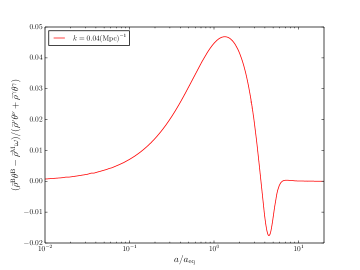
Figure 1: Effects of non-radiation modifying terms compared to the effects of radiation, at $k=0.04$ Mpc^-1 (see Eq. 29). This shows that the non-radiation terms are smaller by more than a factor of $20$.

Putting this together, we find that the GGA effects are almost degenerate with extra radiation, even when we consider perturbations. However, the GGA-$\mathcal{N}_{\rm eff}$ degeneracy does not hold exactly at the perturbation level, since $\delta\rho^{\gamma}/\delta\rho^{\nu}$ and $\theta^{\gamma}/\theta^{\nu}$ are both time- and scale-dependent, contrary to the previous case at the background level, where $\bar{\rho}^{\gamma}/\bar{\rho}^{\nu}$ was a constant number through time and for every scale.

The final test of the modified CAMB code is at the perturbation level when the GA parameter, $G_{\mbox{\tiny{RN}}}$, is not set to zero and GA is fully effective. Based on the discussion in the preceding paragraphs the code should produce the same $C_{\ell}$s for the following two models: ${\cal P}1:=\{G_{\mbox{\tiny{RN}}}=1/3G_{\mbox{\tiny{N}}},\mathcal{N}_{\rm eff}=3.04,T_{0}^{4}=(2.7255)^{4}\}$ and ${\cal P}2:=\{\mbox{GR with}\,\mathcal{N}_{\rm eff}=4/3\times 3.04,\,T_{0}^{4}=4/3\times(2.7255)^{4}\}$, when the non-radiation terms, i.e., terms in $\Delta\omega$ are ignored. We use the value of the present CMB temperature, $T_{0}$, from Ref. Fixsen (2009). However, one needs to be careful while performing this test, since $T_{0}$ appears in many parts of the code that are totally irrelevant to gravity (see Ref. Narimani et al. (2012) for a related discussion), e.g., the sound speed of the plasma before last scattering depends on the photon-to-baryon density ratio and hence on $T_{0}$. Figs. 2 and 3 show these tests of our calculations for GGA. The right panel of these figures tests the code at the perturbation level, while the left panels show the effect of non-radiation fluids on the CMB anisotropies and matter power spectra. Ignoring the effect of non-radiation fluids, is crucial in reducing the GA Eqs. 1–3, to Eq.8 at the perturbation level, and hence the $G_{\mbox{\tiny{RN}}}$–$\zeta_{4}$ correspondence.

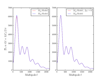
Figure 2: Checking the code at the perturbation level by comparing the matter power spectra for the models ${\cal P}1:=\{G_{\mbox{\tiny{RN}}}=1/3G_{\mbox{\tiny{N}}},\mathcal{N}_{\rm eff}=3.04,T_{0}^{4}=(2.7255)^{4}\}$ and ${\cal P}2:=\{\mbox{GR with}\,\mathcal{N}_{\rm eff}=4/3\times 3.04,\,T_{0}^{4}=4/3\times(2.7255)^{4}\}$ (left panel). There is a small difference between the two at around the first peak. This can be explained by considering the effects of a non-zero $\omega$ (divergence of the aether four-velocity). The two models completely coincide with each other by setting $\Delta\omega$ to zero in the ${\cal P}1$ model (right panel).

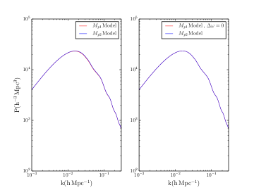
Figure 3: Checking the code at the perturbation level by comparing the the models ${\cal P}1:=\{G_{\mbox{\tiny{RN}}}=1/3G_{\mbox{\tiny{N}}},\mathcal{N}_{\rm eff}=3.04,T_{0}^{4}=(2.7255)^{4}\}$ and ${\cal P}2:=\{\mbox{GR with}\ \mathcal{N}_{\rm eff}=4/3\times 3.04,\,T_{0}^{4}=4/3\times(2.7255)^{4}\}$ (left panel). The small difference between the two can be explained by considering the effects of a non-zero $\omega$. The two models completely coincide with each other by setting $\Delta\omega$ to zero in the ${\cal P}1$ model (right panel).

Figure 4 shows the CMB anisotropy power spectrum predictions from GR and GA (with other GGA models interpolating between the two). The input parameters of the left panel are the same for both theories and are taken from Ref. Planck Collaboration XVI (2013). We see on the left panel that the positions of the peaks are consistently shifted towards smaller scales, i.e., higher $\ell$s. This is because the Universe is younger at recombination in the GA theory, which in turn is due to having effectively more radiation at the background level of the GA theory compared to GR. There is also an enhanced early ISW effect Hu and Sugiyama (1994) in the GA theory due the presence of the the two modifying functions, $B$ and $D$, as was explained before. This can be understood more intuitively using the fact that GA is effectively degenerate at the background and perturbation level with a GR model with one third more radiation. Since the ISW effect is proportional to $e^{-\tau}$ (where $\tau$ is the optical depth), and the time derivative of the metric potentials (that are non-zero only during the matter radiation transition and at very late times), then having more radiation in the Universe will delay the radiation to matter transition to later times with smaller $\tau$ and enhance the ISW effect.

In order for the GA model to match GR and hence fit the data, since there is a very good match between data and GR predictions, one needs to change the matter to radiation density ratio to get the right position for the peaks. This can be done by either deducting from the radiation density, or adding more matter to the GA model. The first option is highly restricted from the CMB temperature data Fixsen (2009). The second option can be done either through adding baryons or cold dark matter, or both. Since the density of baryons is constrained through helium abundance ratio (see e.g. Aver et al. (2010)), the only remaining option is to add cold dark matter to the theory. This is also limited by the ratio of even to odd peaks in the CMB power spectra, but is the last resort! The best fit value for the cold dark matter density in the GA theory, using CMB data only, is: $\Omega_{\rm DM}h^{2}=0.147\pm 0.004$.

After fixing the position of the peaks, one needs to get the right amplitude for the spectra. The relative amplitude of the high-$\ell$ to low-$\ell$ multi-poles is highly affected by the early ISW effect that was explained before and is evident in the left panel of Fig. 4 by comparing the ratio of the power of the two curves in $\ell\sim 250$, and $\ell\sim 2000$. This relative mismatch in the amplitude can be fixed by choosing higher values of the spectral index, $n_{s}$. The best fit value of this parameter in the GA theory is: $n_{s}=1.042\pm 0.008$.

The best-fit predictions of the two theories are compared in the right panel of Fig. 4. We see that the best fit GA theory predicts less power at high $\ell$s compared to GR. The best-fit predictions of the two theories are compared with Planck and SPT data in Fig. 5.

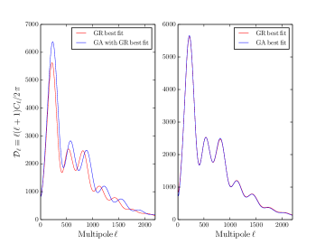
Figure 4: Comparing general relativity versus gravitational aether predictions for the CMB power spectrum. The values of the input parameters for the left panel are taken from the Planck analysis Planck Collaboration XVI (2013). The right panel compares the best-fit predictions of the two theories with all cosmological parameters also allowed to vary. GA predicts less power at higher $\ell$s, as one can see from the right panel.

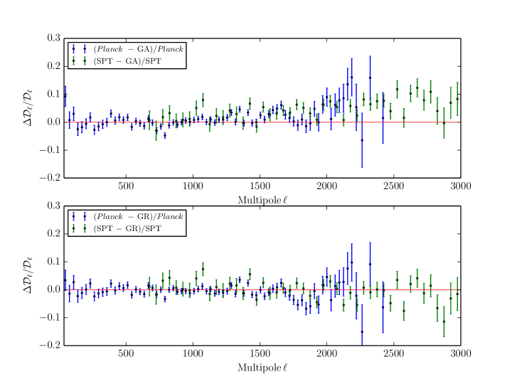
Figure 5: Comparing general relativity (bottom panel) and gravitational aether (top panel) predictions for the CMB power spectrum with Planck and SPT data sets. Here we plot ${\cal D}_{\ell}\equiv\ell(\ell+1)C_{\ell}1/2\pi$ residuals, along with $\pm 1\,\sigma$ error bars, from Refs. Planck Collaboration XVI (2013) and Keisler et al. (2011). While the two theories can both fit the lower-$\ell$ observations, GR fits the data points significantly better than GA for $\ell\gtrsim 1000$, at the ${>}\,4\,\sigma$ level.

III.2 Cosmological constraints

We now turn to deriving precision constraints on GGA from cosmological observations. We assume that $G_{\mbox{\tiny{N}}}$ is equal to the Newtonian gravitational constant measured in Cavendish-type experiments (see e.g.R̃ef. Will (1993)) using sources with negligible pressure. Then CosmoMC can be used for sampling $G_{\mbox{\tiny{R}}}$ using different combinations of the following cosmological data.

1. The first data release of the all-sky CMB temperature anisotropy power spectrum, measured by the Planck Planck Collaboration I (2013) satellite.

2. The 9-year (and final) data release of the WMAP satellite CMB temperature and polarization anisotropy power spectra, which we denote as WMAP-$9$ Hinshaw et al. (2013) (with “WP” indicating the large angle polarization data only).

3. Three seasons of high resolution CMB temperature anisotropy measurements from the ACT experiment Das et al. (2014).

4. $790\,{\rm deg}^{2}$ of high resolution CMB temperature anisotropy measurements from the SPT experiment  Keisler et al. (2011).

5. Sloan Digital Sky Survey (SDSS) Eisenstein et al. (2011) and other estimates of the BAO length scale  Padmanabhan et al. (2012); Anderson et al. (2012); Beutler et al. (2011).

6. The first claimed detection of the amplitude of primordial gravitational waves, based on B-mode polarization anisotropy band-powers detected by the BICEP$2$ experiment at degree scales BICEP2 Collaboration (2014).

There are two special cases of particular interest, which are $G_{\mbox{\tiny{R}}}=G_{\mbox{\tiny{N}}}$ (standard General Relativity; $\zeta_{4}=0$) and $G_{\mbox{\tiny{R}}}=\frac{4}{3}\,G_{\mbox{\tiny{N}}}$ (Gravitational Aether theory; $\zeta_{4}=\frac{1}{3}$). If the data are consistent with the $G_{\mbox{\tiny{R}}}/G_{\mbox{\tiny{N}}}=4/3$ case, or favour this theory over GR, then that would be evidence that GA theory provides a better description of the cosmological data.

Table 1: Mean likelihood values together with the $68\%$ confidence intervals for the usual six cosmological parameters (see Ref. Planck Collaboration XVI (2013)), together with the GGA parameter $G_{\mbox{\tiny{N}}}/G_{\mbox{\tiny{R}}}$. “WP” refers to WMAP-9 polarization, which has been used to constrain the optical depth, $\tau$. “HighL” refers to the higher multipole data sets, ACT and SPT. The PPN parameter, $\zeta_{4}$ can be obtained through $\zeta_{4}=G_{\rm R}/G_{\rm N}-1$.

Table 2: Mean likelihood values together with the $68\%$ confidence intervals for the usual six cosmological parameters, plus $r$ (the tensor-to-scalar ratio), together with the GGA parameter $G_{\mbox{\tiny{N}}}/G_{\mbox{\tiny{R}}}$. The data are as in Table 1, but now including BICEP2 measurements of the B-mode CMB polarization. GR is still favoured over GA if we include HighL CMB or BAO measurements. However, even the conventional seven parameter GR model (that includes $r$), is disfavoured at around the $3\,\sigma$ level when one considers BICEP2, as well as Planck, and HighL data. The PPN parameter, $\zeta_{4}$ can be obtained through $\zeta_{4}=G_{\rm R}/G_{\rm N}-1$.

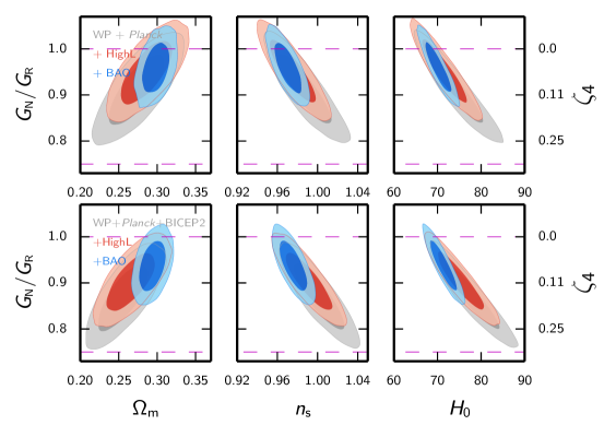
Figure 6: Confidence intervals ($68\%$ and $95\%$) for the GGA parameter and the cosmological parameters it is most degenerate with. The ratio $G_{\rm N}/G_{\rm R}$ is plotted on the left axes and $\zeta_{4}$ on the right axes. The horizontal dashed lines indicate the GR (top line) and GA (bottom line) predictions.

From a broader perspective, any unequal values for $G_{\mbox{\tiny{N}}}$ and $G_{\mbox{\tiny{R}}}$ would be interesting, because this is a way of parameterizing general deviations from the matter-radiation equivalence principle. The MCMC constraints on GGA, excluding the recent BICEP$2$ data release, are summarized in Table  1. It is important to allow the usual cosmological parameters to vary while constraining $G_{\mbox{\tiny{N}}}/G_{\mbox{\tiny{R}}}$. This is because there could be (and indeed are) degeneracies in the new $7$-parameter (or $8$-parameter when the tensor-to-scalar ratio $r$ is included) space. Some of these degeneracies between the GGA parameter, $G_{\mbox{\tiny{N}}}/G_{\mbox{\tiny{R}}}$, and the conventional parameters of cosmology are shown in Fig. 6.

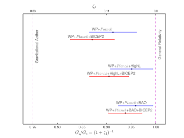
Figure 7: A pictorial comparison of marginalized $G_{\mbox{\tiny{N}}}/G_{\mbox{\tiny{R}}}=(1+\zeta_{4})^{-1}$ measurements. We have plotted the central values and $\pm 1\,\sigma$ error bars using different data sets. The GR and GA predictions are shown as vertical dashed lines.

In fact, we find that if one omits the BICEP2 data, then $G_{\mbox{\tiny{N}}}/G_{\mbox{\tiny{R}}}=1$ provides a good fit and the cosmological parameters hardly shift from their best-fit GR values. On the other hand, adding BICEP$2$ data shifts the results towards GA by about $1\,\sigma$. This may be pointing to some tension in data, or a mild inconsistency between GR and the existing data sets. Of course the most exciting possibility that any such tension is due to missing physics rather than systematic effects. Table  2 shows these constraints, while Fig. 7 presents a pictorial comparison of constraints on $G_{\mbox{\tiny{N}}}/G_{\mbox{\tiny{R}}}$ using different data sets.

IV Discussion

As we can see in Fig. 7, although GR is generally preferred over GA, different combinations of data sets appear to give constraints for the GGA parameter (or anomalous pressure coupling), which are discrepant by as much as 2$\,\sigma$. Perhaps most intriguingly, the combination of Planck temperature anisotropies and polarization from WMAP-9 and BICEP2 (which represents the state of the art for CMB anisotropy measurements above $0.1^{\circ}$), lies about mid-way between the GA and GR predictions (with a preference for GA, but only at the level of $\Delta\chi^{2}\,{\simeq}\,1$). Nevertheless, the best fit for $G_{\rm N}/G_{\rm R}$ is inconsistent with both GA and GR at 2.7 and 2.9$\,\sigma$, respectively. The latter is a manifestation of the well-known tension between the Planck upper limit on tensor modes, and the reported detection by BICEP2 (at least for standard $\Lambda$CDM cosmology with a power-law primordial power spectrum).

Let us now try to qualitatively understand what might be responsible for the different trends that we observe when fitting different data sets, as we turn up the GGA parameter. The first step is to obtain the gross structure of the CMB $C_{\ell}^{\rm TT}$ power spectrum peaks by fixing $\theta$, the ratio of the sound horizon at last scattering, to the distance to the last-scattering surface. For any value of $G_{\rm N}/G_{\rm R}$, this can be done by picking appropriate values of $\Omega_{m}$ and $h$, which explains the degeneracy directions in Fig. 7 for these parameters.

The next step is to recognize the effect of free steaming on the damping tail of the CMB power spectrum. Similar to the effect of free streaming of additional neutrinos, boosting the gravitational effect of neutrinos leads to additional suppression of power at small scales, or high $\ell$, in the CMB power spectrum,as we can see in Fig. 5. This can be partially compensated for by increasing the spectral index of the scalar perturbations, leading to a bluer primordial spectrum. In fact, we see that combinations of data sets that prefer larger $G_{\rm R}$ (in Tables 1–2) prefer a near scale-invariant power spectrum, $n_{\rm s}\simeq 1$ (which is up from the value $n_{\rm s}\simeq 0.96$ in GR+$\Lambda$CDM).

Finally, a bluer scalar spectral index tends to suppress scalar power for $\ell\lesssim 100$, which then relaxes the upper bound on tensors from the Planck temperature power spectrum. This allows a higher value of $r$ than the limit ($r<0.11$ Planck Collaboration XVI (2013)) found from the temperature anisotropies in $\Lambda$CDM.

Of course, none of these degeneracies are perfect. In particular, the additional damping due to free-streaming is much steeper than a power law, which is why even the best-fit GA model underpredicts CMB power for $\ell\gtrsim 1000$ in Fig. 5. This is also why adding higher resolution CMB observations (from ACT and SPT), pushes the best fit away from GA. It is possible that adding a positive running for the spectral index might be able to partially cancel the effect, at least for the observable range of multipoles. However, a significant positive running would be hard to justify in simple models of inflation, and may also exacerbate the observational tensions with structure formation on small scales in $\Lambda$CDM.

A more stringent constraint on GA (and thus anomalous pressure coupling) comes from the degeneracy with the Hubble constant, which can also be seen in Fig. 6. Additional gravitational coupling to pressure, of the sort required in GA, requires $H_{0}>80\,{\rm km}\,{\rm s}^{-1}\,{\rm Mpc}^{-1}$, which is larger than even the highest measurements in the current literature (see e.g., figure 16 in Ref. Planck Collaboration XVI (2013)). In particular, BAO geometric constraints place tight bounds of $H_{0}\simeq 68$–$72\,{\rm km}\,{\rm s}^{-1}\,{\rm Mpc}^{-1}$, which is why the inclusion of these data substantially cuts off the smaller values of $G_{\rm N}/G_{\rm R}$. However, we should note that this inference is based on a simple cosmological constant model for dark energy at low redshifts; more complex descriptions of dark energy, as suggested by some recent BAO Delubac et al. (2014) or Supernovae Ia Rest et al. (2013) studies, could relax these $H_{0}$ constraints.

There are certainly hints of possible systematics among the different data sets that could explain some of these tensions. For example, the power spectrum of WMAP-9 appears to be about 2.5% higher than Planck Planck Collaboration XVI (2013); Kovács et al. (2013), independent of scale. Additionally, the first 30 or so multipoles appear low (in both WMAP and Planck data), which, coupled with calibration, can affect the best fit in the damping tail. A perhaps related issue is that the best-fit lensing amplitude in Planck and Planck+HighL spectra, appears to be around 20% higher than expected in the $\Lambda$CDM model Planck Collaboration XVI (2013); Beutler et al. (2014). Since lensing moves power from small $\ell$s to high $\ell$s, this could also have an indirect effect on the shape of the high-$\ell$ power spectrum.

Finally, there are legitimate questions about whether BICEP2 analysis BICEP2 Collaboration (2014) has underestimated the effect of instrumental systematics or Galactic foregrounds (e.g., Liu et al. (2014)). Decreasing the primordial amplitude of B-modes would reduce the tension with Planck, and thus relax the need for anomalous pressure coupling (i.e., $G_{\rm N}<G_{\rm R}$).

On balance it seems premature to claim that $\zeta_{4}>0$ is required by the current cosmological data. The simple GA theory (with $\zeta_{4}=1/3$) certainly appears disfavoured by the data. However, as the quality of the data continue to improve, it is worth bearing in mind that the GGA picture provides a particular degree of freedom. This should be considered in future fits, particularly with the upcoming release of the Planck polarization data.

V Conclusions, and Open Questions

In this paper, we have closely examined the question of anomalous pressure coupling to gravity in cosmology. This was done in the context of the Generalized Gravitational Aether framework, which allows for an anomalous sourcing of gravity by pressure ($\zeta_{4}$ in the PPN framework), while not affecting other precision tests of gravity. The idea would mean that the gravitational constant during the radiation era, when $p=\frac{1}{3}\rho$, is boosted to $G_{\rm R}=(1+\zeta_{4})G_{\rm N}$, compared to the gravitational constant for non-relativistic matter $G_{\rm N}$. In particular, the case with $\zeta_{4}=1/3$ or $G_{\rm R}=4G_{\rm N}/3$, can be used to decouple vacuum energy from gravity, and thus solve the (old) cosmological constant problem.

We have implemented cosmological linear perturbations for this theory into the code CAMB, and explored the models that best fit different combinations of cosmological data. The effects are qualitatively similar to introducing additional neutrinos ($N_{\rm eff}$), or dark radiation. Our constraints are summarized in Tables 1–2 and Figs. 6–7.

There is clearly some mild tension between different data combinations, but $\zeta_{4}=1/3$ is inconsistent with current observations at around the 2.6-$-5\,\sigma$ level, depending on the combination used. CMB B-mode observations (from BICEP2) push for larger $\zeta_{4}$, while high resolution CMB or baryonic acoustic oscillations, go in the opposite direction. The best fit is in the range $0.04\lesssim\zeta_{4}\lesssim 0.15$, or $0.87\lesssim G_{\rm N}/G_{\rm R}\lesssim 0.96$, with statistical errors of a half to third of this range. It may be interesting to notice that even GR ($\zeta_{4}=0$) is disfavoured at $3\,\sigma$ when we combine lower resolution CMB observations.

To bring some statistical perspective, we should note that even if the gravitational aether solution to the cosmological constant problem is ruled out at $5\,\sigma$, the standard GR+$\Lambda$CDM paradigm, with no fine-tuning, is ruled out at ${>}\,10^{60}\,\sigma$! Therefore, while the first attempt at solving the problem might not have been entirely successful (compared to a model that takes the liberty of fine-tuning the vacuum energy), we argue, that it may be a step in the right direction. So, other than working to improve the quality and consistency of observational data, what can we do to tackle this problem, that quantum fluctuations appear not to gravitate?

From the theoretical standpoint, there are several clear avenues that we have already alluded to:

1. As we discussed in the Introduction, gravitational aether is a classical theory for an effective low energy description of gravity. Therefore, like all effective theories, it has an energy cut-off above which it will not be valid. In fact, the length-scale $\lambda_{\rm c}$ (inverse energy scale) associated with this cut-off should be $\lambda_{\rm c}\sim 0.1$ mm, since a smaller $\lambda_{\rm c}$ would not fully solve the cosmological constant problem, while larger $\lambda_{\rm c}$ could have been seen in torsion balance tests of gravity (although it is not entirely clear what the signature would be). It is worth noting that the number density of baryons at CMB last scattering is $0.33\,{\rm mm}^{-3}$, implying that to calculate $T^{\alpha}_{\alpha}$ in Eq. 1, it might be necessary to use a microscopic description of atoms interacting with aether, as opposed to the usual mean fluid density picture . If this is the case, then each microscopic particle would carry an aether halo of size about $\sim\lambda_{\rm c}$; this would appear like a renormalization of particle mass for all macroscopic gravitational effects, but otherwise (like for other vacuum tests of gravity), the theory would be indistinguishable from GR. Nevertheless, in lieu of a quantum theory of gravitational aether, it is not clear how much progress can be made in this direction.

2. Another possibility is to modify the simple ansatz (2) for the energy-momentum tensor of the gravitational aether, e.g., by introducing a density, $\rho^{\prime}$. This might be a reasonable approach if one is also attempting to connect gravitational aether to dark energy (which does have both density and pressure at late times). However, Eq. 3 will no longer be sufficient to predict the evolution of the aether, and thus we would need another equation to fix the aether equation of state.

3. In solving for the evolution of aether with respect to dark matter, $\omega$, we have assumed that the two substances were originally comoving, i.e., $\omega=0$ at early times. However, depending on the process that generates primordial scalar fluctuations in this picture, $\omega$ could have also been sourced in the early Universe. So, even though its amplitude decays as $a^{-1}$ on super-horizon scales, depending on its amplitude and spectrum, it can impact CMB observations. This would be akin to introducing isocurvature modes, but for aether perturbations. Although, since $\omega$ decays exponentially on sub-horizon scales, this could only affect the CMB at $\ell\lesssim 100$.

4. Finally, we have not included the effect of neutrino mass in our GGA treatment. Massive neutrinos will be qualitatively different from other components, as they start as radiation, which does not couple to aether, but then gradually start sourcing aether as they become non-relativistic. However, this happens relatively late in cosmic history, long after CMB last-scattering, and when neutrinos make up only a small fraction of cosmic density. Therefore, although this would be a useful direction to pursue, we do not expect a significant change from the analyses presented here.

In contrast to unfalsifiable approaches for solving the cosmological constant problem, such as landscape/multiverse ideas with anthropic arguments, the gravitational aether concept has the very distinct advantage of being predictive and hence it can be falsified. Here, we have demonstrated this explicitly, since the basic picture does not appear to fit the current cosmological data. However, like elsewhere in physics, the logical next step would be to learn from this process and propose better physical models (rather than relying on metaphysics). We believe that the GGA approach yields a useful parameterization of a particular degree of freedom in models of modified gravity, and that this idea is worth pursuing further.

References

- Weinberg (1989) S. Weinberg, Reviews of Modern Physics 61, 1 (1989).
- Straumann (2003) N. Straumann, in XVIIIth IAP Colloquium: Observational and theoretical results on the accelerating universe (2003) arXiv:gr-qc/0208027 .
- Riess et al. (1998) A. G. Riess, A. V. Filippenko, and et. al., Astronomy Journal 116, 1009 (1998), arXiv:astro-ph/9805201 .
- Perlmutter et al. (1999) S. Perlmutter, G. Aldering, and et. al., Astrophys. J. 517, 565 (1999), arXiv:astro-ph/9812133 .
- Afshordi (2008) N. Afshordi, (2008), arXiv:0807.2639 .
- Aslanbeigi et al. (2011) S. Aslanbeigi, G. Robbers, and et. al., Phys. Rev. D 84, 103522 (2011), arXiv:1106.3955 .
- Zel’dovich (1968) Y. B. Zel’dovich, Soviet Physics Uspekhi 11, 381 (1968).
- Thomas et al. (2009) E. C. Thomas, F. R. Urban, and A. R. Zhitnitsky, Journal of High Energy Physics 8, 043 (2009), arXiv:0904.3779 [gr-qc] .
- Prescod-Weinstein et al. (2009) C. Prescod-Weinstein, N. Afshordi, and M. L. Balogh, Phys. Rev. D 80, 043513 (2009), arXiv:0905.3551 .
- Will (2014) C. M. Will, (2014), arXiv:1403.7377 .
- Will (1976) C. M. Will, Astrophys. J. 204, 224 (1976).
- Kapner et al. (2007) D. J. Kapner, T. S. Cook, and et. al., Physical Review Letters 98, 021101 (2007), arXiv:hep-ph/0611184 .
- Schwab et al. (2008) J. Schwab, S. A. Hughes, and S. Rappaport, ArXiv e-prints (2008), arXiv:0806.0798 .
- Kamiab and Afshordi (2011) F. Kamiab and N. Afshordi, Phys. Rev. D 84, 063011 (2011), arXiv:1104.5704 .
- Rappaport et al. (2008) S. Rappaport, J. Schwab, S. Burles, and G. Steigman, Phys. Rev. D 77, 023515 (2008), arXiv:0710.5300 .
- Hinshaw et al. (2013) G. Hinshaw, D. Larson, and et. al., ApJS 208, 19 (2013), arXiv:1212.5226 .
- Planck Collaboration et al. (2011) Planck Collaboration, P. A. R. Ade, N. Aghanim, M. Arnaud, M. Ashdown, J. Aumont, C. Baccigalupi, M. Baker, A. Balbi, A. J. Banday, and et al., A&A 536, A1 (2011), arXiv:1101.2022 [astro-ph.IM] .
- Das et al. (2014) S. Das, T. Louis, and et. al., JCAP 4, 014 (2014), arXiv:1301.1037 .
- Keisler et al. (2011) R. Keisler, C. L. Reichardt, and et. al, Astrophys. J. 743, 28 (2011), arXiv:1105.3182 .
- Ma and Bertschinger (1995) C.-P. Ma and E. Bertschinger, Astrophys. J. 455, 7 (1995), arXiv:astro-ph/9506072 .
- Narimani and Scott (2013) A. Narimani and D. Scott, Phys. Rev. D 88, 083513 (2013), arXiv:1303.3197 .
- Sachs and Wolfe (1967) R. K. Sachs and A. M. Wolfe, Astrophys. J. 147, 73 (1967).
- Lewis et al. (2000) A. Lewis, A. Challinor, and A. Lasenby, Astrophys. J. 538, 473 (2000), arXiv:astro-ph/9911177 .
- Lewis and Bridle (2002) A. Lewis and S. Bridle, Phys. Rev. D 66, 103511 (2002), arXiv:astro-ph/0205436 .
- Fixsen (2009) D. J. Fixsen, Astrophys. J. 707, 916 (2009), arXiv:0911.1955 [astro-ph.CO] .
- Narimani et al. (2012) A. Narimani, A. Moss, and D. Scott, Astrophysics and Space Science 341, 617 (2012), arXiv:1109.0492 .
- Planck Collaboration XVI (2013) Planck Collaboration XVI, A&A (2013), arXiv:1303.5076 .
- Hu and Sugiyama (1994) W. Hu and N. Sugiyama, Phys. Rev. D 50, 627 (1994), arXiv:astro-ph/9310046 .
- Aver et al. (2010) E. Aver, K. A. Olive, and E. D. Skillman, JCAP 5, 003 (2010), arXiv:1001.5218 [astro-ph.CO] .
- Will (1993) C. M. Will, Theory and Experiment in Gravitational Physics, by Clifford M. Will, pp. 396. ISBN 0521439736. Cambridge, UK: Cambridge University Press, March 1993. (Cambridge University Press, 1993).
- Planck Collaboration I (2013) Planck Collaboration I, A&A (2013), arXiv:1303.5062 .
- Eisenstein et al. (2011) D. J. Eisenstein, D. H. Weinberg, and et al., Astrophysical Journal 142, 72 (2011), arXiv:1101.1529 .
- Padmanabhan et al. (2012) N. Padmanabhan, X. Xu, and et al., MNRAS 427, 2132 (2012), arXiv:1202.0090 .
- Anderson et al. (2012) L. Anderson, E. Aubourg, and et al., MNRAS 427, 3435 (2012), arXiv:1203.6594 .
- Beutler et al. (2011) F. Beutler, C. Blake, and et al., MNRAS 416, 3017 (2011), arXiv:1106.3366 .
- BICEP2 Collaboration (2014) BICEP2 Collaboration, (2014), arXiv:1403.3985 .
- Delubac et al. (2014) T. Delubac, J. E. Bautista, and et. al., (2014), arXiv:1404.1801 .
- Rest et al. (2013) A. Rest, D. Scolnic, and et. al., (2013), arXiv:1310.3828 .
- Kovács et al. (2013) A. Kovács, J. Carron, and I. Szapudi, MNRAS 436, 1422 (2013), arXiv:1307.1111 .
- Beutler et al. (2014) F. Beutler, S. Saito, and et. al., (2014), arXiv:1403.4599 .
- Liu et al. (2014) H. Liu, P. Mertsch, and S. Sarkar, (2014), arXiv:1404.1899 .