Plane shear flows of frictionless spheres: Kinetic theory and 3D Soft-Sphere Discrete Element Method simulations

Abstract

We use existing 3D Discrete Element simulations of simple shear flows of spheres to evaluate the radial distribution function at contact that enables kinetic theory to correctly predict the pressure and the shear stress, for different values of the collisional coefficient of restitution. Then, we perform 3D Discrete Element simulations of plane flows of frictionless, inelastic spheres, sheared between walls made bumpy by gluing particles in a regular array, at fixed average volume fraction and distance between the walls. The results of the numerical simulations are used to derive boundary conditions appropriated in the cases of large and small bumpiness. Those boundary conditions are, then, employed to numerically integrate the differential equations of Extended Kinetic Theory, where the breaking of the molecular chaos assumption at volume fraction larger than 0.49 is taken into account in the expression of the dissipation rate. We show that the Extended Kinetic Theory is in very good agreement with the numerical simulations, even for coefficients of restitution as low as 0.50. When the bumpiness is increased, we observe that some of the flowing particles are stuck in the gaps between the wall spheres. As a consequence, the walls are more dissipative than expected, and the flows resemble simple shear flows, i.e., flows of rather constant volume fraction and granular temperature.

I Introduction

Granular materials are collections of discrete particles characterized by loss of energy whenever the particles interact. Their mechanical behavior is very complex even in the case of simple flow conditions (i.e., elementary geometries, stationary motions) or when the granular matter is particularly treatable (i.e., dry, no complex shapes of the grains and no polydispersity, etc). Due to their microscopic, discrete nature and their macroscopic behavior, granular materials are treated in both the frameworks of discontinuum (Discrete Element simulations) and continuum mechanics. Among the latter, kinetic theories of granular gases represent the most fundamental approach.
Classic kinetic theories have been derivedJenkins and Savage (1983); Lun (1991); Garzó and Dufty (1999); Goldhirsch (2003) assuming that the energy of the system is dissipated through binary, instantaneous collisions between smooth spheres, and have been proved to succeed at low to moderate solid volume fractions. When the granular material becomes denser, the assumption of chaotic, binary, instantaneous collisions fails;Campbell (2002); Mitarai and Nakanishi (2007); Kumaran (2009) also, force chains can develop within the medium.Majmudar and Behringer (2005); da Cruz et al. (2005) Several modifications to the classic kinetic theories have been recently proposed, in order to take into account the role of velocity correlation Jenkins (2006, 2007) and the development of force chains.Johnson and Jackson (1987, 1990); Louge (2003); Berzi, di Prisco, and Vescovi (2011); Vescovi, di Prisco, and Berzi (2013)
The steady plane shear flow of granular materials, in absence of gravity and pressure gradient, serves as test case for the theories. Numerical simulations of simple shear flows (i.e., characterized by homogeneous shearing obtained by imposing the Lees-Edwards Lees and Edwards (1972) periodic boundary conditions in the shearing direction) of disks or spheres have been performed using Event-Driven molecular dynamics (ED) and the Soft-Sphere Discrete Element Method (SS-DEM).da Cruz et al. (2005); Ji and Shen (2006); Mitarai and Nakanishi (2007); Chialvo and Sundaresan (2013) Inhomogeneous shearing can be obtained in numerical simulations Shojaaee et al. (2012); Karion and Hunt (2000); Liu and Rosato (2005); Xu, Louge, and Reeves (2003) and physical experiments Orlando and Shen (2012); Miller et al. (ress) when the granular material is sheared between two solid parallel planes, one at rest and the other moving at constant velocity. In this paper, we numerically solve the Extended Kinetic Theory (EKT), in the form proposed by Berzi (2014), for wall-bounded, plane shear granular flows of identical, frictionless spheres, and compare the field variables profiles with those obtained by performing 3D SS-DEM simulations. The boundaries are made bumpy by gluing spheres, identical to the moving particles, at the walls; the inter-particle collisions are characterized by the coefficient of restitution, $e$, the ratio of the relative velocity between two impending particles after and before a collision. We first use existing numerical results on simple shear flows to slightly modify the constitutive relations of EKT, and then, we analyze both the influence of the coefficient of restitution and the bumpiness. Recently, also Chialvo and Sundaresan (2013) have proposed corrections to the kinetic theory of Garzó and Dufty (1999) on the basis of 3D SS-DEM simulations of simple shear flows of frictionless and frictional spheres. The main differences between our work and theirs are: (i) we focus on flows where the influence of the boundaries cannot be neglected and propose corrections to the boundary conditions originally developed for nearly elastic spheres glued at the walls Richman (1988) for two extreme values of the bumpiness; (ii) we propose a different radial distribution function obtained from a combination of the classic Carnahan and Starling (1969)’s and Torquato (1995)’s expressions, which fits also the numerical data of Chialvo and Sundaresan (2013); (iii) we use an expression for the correlation length recently obtained from the analysis of ED simulations of simple shear flows Berzi (2014) which does not require additional parameters besides the coefficient of restitution; (iv) unlike Chialvo and Sundaresan (2013), we show that there is no need for correcting the constitutive relation of the shear stress, provided that the coefficient of restitution is lower than 0.95.
The paper is organized as follows. In Sec. II we introduce the EKT and the boundary conditions. Sec. III is devoted to describe the simulation method. In Sec. IV we derive the definition of a new radial distribution function and compare the results of the SS-DEM simulations with those obtained from the numerical integration of the equations of EKT. Finally, concluding remarks are summarized in Sec. V.

II Governing equations

We focus on the steady motion of a mixture of identical, frictionless spheres sheared between two parallel planes, one at rest and the other moving at constant velocity $V$ (Fig. 1).

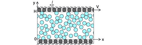
Figure 1: Sketch of the constant-volume wall-bounded plane shear flow configuration. A granular material confined between two horizontal solid planes is sheared by moving one plane at constant velocity $V$ ($x$ are $y$ are respectively the flow and shear directions). The two planes are made bumpy by gluing grains at their surface in a regular hexagonal array, where $l$ is the distance between the edges of two adjacent spheres.

We take $x$ and $y$ to be the flow and the shearing directions, respectively, and ignore variations along the transversal direction $z$. In what follows, all the quantities are made dimensionless using the particle diameter $d$ and density $\rho_{p}$ and the wall velocity $V$. Spheres having the same properties of the moving particles are glued at the walls in a regular hexagonal array, where $l$ is the distance between the edges of two adjacent spheres. The bumpiness of the wall is measured by $\psi$, with $\sin\psi=(1+l)/2$.Richman (1988) We take $y=0$ to be at the top of the particles glued at the resting wall, and $y=H$ to be at the bottom of the particles glued at the moving wall.

The hydrodynamic mean fields are the solid volume fraction $\nu$, the velocity along the $x$ direction $u$, the pressure $p$ and the shear stress $s$. For frictionless particles, momentum is exchanged only through collisions,Vescovi, di Prisco, and Berzi (2013) and a description based on kinetic theory Jenkins and Savage (1983); Lun (1991); Goldhirsch (2003) is suitable. We adopt a constant coefficient of restitution $e$. The continuous velocity field is first coarsed-grained at the scale of a grain diameter. The mean square of the velocity fluctuations against this field, averaged at the same scale, then defines a “granular temperature” $T$ field, which measures the degree of agitation of the system.
In the absence of external forces, and in steady conditions, the momentum balance trivially asserts that the pressure and the shear stress are constant along $y$. The balance of the fluctuating energy reads

$$su^{\prime}=Q^{\prime}+\Gamma.$$ (1)

where $Q$ is the fluctuating energy flux and $\Gamma$ is the rate of dissipation associated to collisions. Here and in what follows, a prime indicates the derivative with respect to the $y$ direction. In order to close the problem, we need constitutive relations for $p$, $s$, $Q$ and $\Gamma$. Kinetic theory (e.g., Garzó and Dufty, 1999) gives

$$p=f_{1}T,$$ (2)

$$s=f_{2}T^{1/2}u^{\prime},$$ (3)

$$\Gamma=\dfrac{f_{3}}{L}T^{3/2},$$ (4)

and

$$Q=-f_{4}T^{1/2}T^{\prime}-f_{5}T^{3/2}\nu^{\prime},$$ (5)

where $f_{1},f_{2},f_{3},f_{4}$ and $f_{5}$ are explicit functions of the volume fraction and the coefficient of restitution and are listed in Tab. 1. There, $g_{0}$ is the radial distribution function, whose expression is given in section IV on the basis of numerical results. In Eq. (4), $L$ is the correlation length, which accounts for the decrease in the rate of collisional dissipation due to the correlated motion of particles that occurs at large volume fraction.Mitarai and Nakanishi (2007); Kumaran (2009) Taking into account this effect, i.e., the breaking of the molecular chaos assumption, is the peculiarity of EKT.Jenkins (2006, 2007); Jenkins and Berzi (2010); Berzi and Jenkins (2011); Jenkins and Berzi (2012); Berzi (2014) The expression for $L$ has been suggested by Jenkins Jenkins (2007) on the basis of a simple heuristic argument,

$$L=\max\left(1,L^{*}\dfrac{u^{\prime}}{T^{1/2}}\right),$$ (6)

where $L^{*}$ is a function of the volume fraction and the coefficient of restitution. When $L$ is equal to one, the molecular chaos assumption is valid and EKT reduces to classic kinetic theory. Berzi (2014) has suggested an expression for $L^{*}$ on the basis of previous results of ED simulations of simple shear flows:

$$L^{*}=\left(\dfrac{f_{2}}{f_{3}}\right)^{1/2}\left[\dfrac{2\left(1-e\right)}{15}\left(g_{0}-g_{0,{\mbox{\scriptsize f}}}\right)+1\right]^{3/2},$$ (7)

where $g_{0,{\mbox{\scriptsize f}}}$ is the value of $g_{0}$ at the freezing point, $\nu=0.49$, i.e., the lowest value of the volume fraction for which a transition to an ordered state is first possible. Torquato (1995)

Table 1: List of auxiliary coefficients in the constitutive relations of kinetic theory.

$f_{1}=$	$4\nu GF$
$f_{2}=$	$\dfrac{8J}{5\pi^{1/2}}\nu G$
$f_{3}=$	$\dfrac{12}{\pi^{1/2}}\left(1-e^{2}\right)\nu G$
$f_{4}=$	$\dfrac{4M\nu G}{\pi^{1/2}}$
$f_{5}=$	$\dfrac{25\pi^{1/2}N}{128\nu}$
$G=$	$\nu g_{0}$
$F=$	$\dfrac{1+e}{2}+\dfrac{1}{4G}$
$J=$	$\dfrac{1+e}{2}+\dfrac{\pi}{32}\dfrac{\left[5+2(1+e)(3e-1)G\right]\left[5+4(1+e)G\right]}{\left[24-6\left(1-e\right)^{2}-5(1-e^{2})\right]G^{2}}$
$M=$	$\dfrac{1+e}{2}+\dfrac{9\pi}{144\left(1+e\right)G^{2}}\dfrac{\left[5+3G\left(2e-1\right)\left(1+e\right)^{2}\right]\left[5+6G\left(1+e\right)\right]}{16-7\left(1-e\right)}$
$N=$	$\dfrac{96\nu\left(1-e\right)}{25G\left(1+e\right)}\dfrac{5+6G\left(1+e\right)}{16+3\left(1-e\right)}\times$
	$\left\{\dfrac{20\nu H\left[5+3G\left(2e-1\right)\left(1+e\right)^{2}\right]}{48-21\left(1-e\right)}-e\left(1+e\right)G\left(1+\nu H\right)\right\}$
$H=$	$\dfrac{1}{G}\dfrac{dG}{d\nu}$

From the constitutive relations for the shear stress (3) and the pressure (2), we obtain the differential equation governing the velocity,

$$u^{\prime}=\dfrac{s}{p}\dfrac{f_{1}}{f_{2}}T^{1/2}.$$ (8)

By deriving Eq. (2) and using Eq. (5), the differential equation for the volume fraction results

$$\nu^{\prime}=\dfrac{Q}{T^{1/2}}\dfrac{f_{1}^{2}}{f_{4}}\left[pf_{1,\nu}\left(1-\dfrac{f_{5}f_{1}}{f_{4}f_{1,\nu}}\right)\right]^{-1},$$ (9)

where $f_{1,\nu}$ represents the derivative of $f_{1}$ with respect to the volume fraction. Finally, using Eqs. (1), (2), (4) and (8), the differential equation for the energy flux reads

$$Q^{\prime}=pT^{1/2}\left[\dfrac{f_{1}}{f_{2}}\left(\dfrac{s}{p}\right)^{2}-\dfrac{f_{3}}{Lf_{1}}\right].$$ (10)

We also introduce an additional differential equation for the partial mass hold-up, defined as $m=\int_{0}^{y}\nu dz$,

$$m^{\prime}=\nu.$$ (11)

Then, the value of the average volume fraction $\bar{\nu}$ along $y$ can be implemented as a boundary condition for $m$.

We numerically solve the set of the four differential equations Eqs. (8)-(11) using the function ‘bvp4c’ implemented in MATLAB, and fixing the gap $H$. We treat the pressure and the shear stress as parameters, so that we need six boundary conditions to solve the problem. As already mentioned, we implement the fixed average volume fraction as a boundary condition for the partial mass hold-up, i.e., $m_{H}=\bar{\nu}H$, while, at the resting wall, $m_{0}=0$. Here and in what follows, the index represents the coordinate $y$ at which the quantity is evaluated. We allow the particles to slip at the bumpy walls, so that, for symmetry, $u_{0}=u_{w}$ and $u_{H}=1-u_{w}$, where Richman (1988) obtained, in the case of rigid, nearly elastic semi-spheres attached to a flat wall,

$$u_{w}=\sqrt{\dfrac{\pi}{2}}h\dfrac{s}{p}T_{0}^{1/2},$$ (12)

with

$$h=\dfrac{2}{3}\dfrac{\left[1+\dfrac{5F_{0}\left(1+B\right)\sin^{2}\psi}{2\sqrt{2}J_{0}}\right]}{\dfrac{2\left(1-\cos\psi\right)}{\sin^{2}\psi}}+\dfrac{5F_{0}}{\sqrt{2}J_{0}},$$ (13)

where $B=\pi\left[1+5/\left(8G_{0}\right)\right]/\left(12\sqrt{2}\right)$, and $J_{0}$, $F_{0}$ and $G_{0}$ are obtained from the corresponding expressions of Tab. 1 with $\nu=\nu_{0}$. The bumpy walls act either as a sink or a source of fluctuating energy to the system. The two boundary conditions for the energy flux are $Q_{0}=Q_{w}$ and $Q_{H}=-Q_{w}$, where Richman (1988) proposed

$$Q_{w}=su_{w}-\sqrt{\dfrac{\pi}{2}}pT_{0}^{1/2}(1-e)\dfrac{2\left(1-\cos\psi\right)}{\sin^{2}\psi}.$$ (14)

The results of the numerical integration will be compared with those obtained from SS-DEM simulations described in Sec. III.

III SS-DEM Simulations

We have carried out 3D SS-DEM simulations using our own code Brodu, Richard, and Delannay (2013) to make comparisons with the results of EKT. Although this method is well known and can be found in many papers,Silbert et al. (2001); Taberlet, Richard, and Delannay (2008); Taberlet and Richard (2006); Rycroft, Orpe, and Kudrolli (2009); Majmudar et al. (2007); Hirshfeld and Rapaport (2001); Richard, McNamara, and Tankeo (2012); Richard et al. (2008) we present it here to support our discussion on the comparison of numerical and theoretical results (Fig. 2).

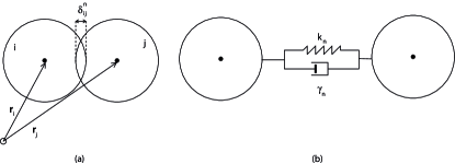
Figure 2: Sketches of two particles at contact (a) and of the contact forces used (b)

In this method, each grain $i$ is a soft sphere of diameter $d_{i}$, mass $m_{i}$, moment of inertia $I_{i}$, position $\mathbf{r}_{i}$, velocity $\mathbf{v}_{i}$ and angular velocity ${\bm{\omega}}_{i}$. For a pair of particles $\left\{i,j\right\}$, we define the relative distance vector $\mathbf{r}_{ij}=\mathbf{r}_{i}-\mathbf{r}_{j}$, their separation $r_{ij}=\left|{\mathbf{r}}_{ij}\right|$, the relative velocity ${\mathbf{v}}_{ij}={\mathbf{v}}_{i}-{\mathbf{v}}_{j}$, and the normal unit vector ${\mathbf{n}}_{ij}=({\mathbf{r}}_{i}-{\mathbf{r}}_{j})/r_{ij}$. These two particles are in contact if their normal overlap $\delta_{ij}^{n}=\mbox{max}(0,d_{i}/2+d_{j}/2-r_{ij})$ is strictly positive. In general, the force on particle $i$ from the interaction with particle $j$ is the sum of a normal and tangential contribution : $\mathbf{f}_{ij}=\mathbf{f}^{n}_{ij}+\mathbf{f}^{t}_{ij}.$ However, the present work deals with frictionless particles for which the contact force is purely normal. Therefore, the grains are submitted to neither tangential forces nor torques. For the normal force, we use the standard spring-dashpot interaction model:Luding (2008) $\mathbf{f}^{n}_{ij}=k_{n}\delta_{ij}^{n}\mathbf{n}_{ij}-\gamma_{n}\mathbf{v}_{ij}^{n},$ where $k_{n}$ is the spring constant, $\gamma_{n}$ the damping coefficient and $\mathbf{v}_{ij}^{n}$ the normal relative velocity $\mathbf{v}_{ij}^{n}=(\mathbf{v}_{ij}\cdot\mathbf{n}_{ij})\mathbf{n}_{ij}.$ The damping is used to obtain an inelastic collision. For a purely normal collision, the collision time $t_{c}$ is equal to $\pi/\left[k_{n}/m_{ij}-\gamma_{n}^{2}/\left(4m_{ij}^{2}\right)\right]^{1/2}$, with the reduced mass $m_{ij}=m_{i}m_{i}/(m_{i}+m_{j})$. The normal restitution coefficient is given by $e=\exp\left[-t_{c}\gamma_{n}/(2m_{ij})\right].$ The total force on particle $i$ is then a combination of contact forces with other particles and the boundaries and an eventual resulting external force $\mathbf{F}_{ext}$. The resulting force $\mathbf{f}_{i}$ is given by

$$\mathbf{f}_{i}=\mathbf{F}_{ext}+\sum_{j=1,j\neq i}^{N}\mathbf{f}_{ij},$$

where $N$ is the total number of flowing spheres. Once the forces are calculated for all the particles, the Newton’s equations of motion, $m_{i}{d^{2}\mathbf{r}_{i}}/{dt^{2}}=\mathbf{f}_{i}$, for the translational degrees of freedom are integrated. We use a velocity Verlet integration scheme with a time step $\Delta t=t_{c}/30$. The grains have all the same size and density. As already mentioned, the numerical results are given in nondimensional units: distances, times, velocities, forces, elastic constants and viscoelastic constants are, respectively, measured in units of $d$, $d/V$, $V$, $\rho_{p}d^{2}V^{2}$, $\rho_{p}dV^{2}$ and $\rho_{p}d^{2}V$.
All the simulations have been performed in a rectangular box of length $L_{x}=20$, width $L_{z}=10$ and height $L_{y}=20$ - so that $H=L_{y}-2=18$ - with $N=3132$. The bumpiness has been generated by gluing, in a regular hexagonal array, a total of 340 particles at the two walls in the case of $\psi=\pi/5$, and 154 in the case $\psi=\pi/3$. Hence, taking into account the extra-space accessible to any flow particle in between the wall-spheres, $\bar{\nu}=0.45$ when $\psi=\pi/5$ and $\bar{\nu}=0.44$ when $\psi=\pi/3$. The particle stiffness of the linear spring model has been set equal to $2\cdot 10^{5}$. The non-dimensional ratio of the particle stiffness over the particle pressure is greater than $10^{5}$ in all the simulations. This ensures that the contact time during a collision is much less than the flight time in between two successive collisions, so that the latter can be considered instantaneous.Otsuki, Hayakawa, and Luding (2010); Berzi, di Prisco, and Vescovi (2011) The value of $\gamma_{n}$ is adjusted to obtain the chosen normal restitution coefficient. Periodic boundary conditions are employed in the $x$ and $z$ directions and the horizontal flat walls are located at $y=-1$ and $y=H+1$, the latter moving at constant horizontal velocity $V$. Those walls are treated as spheres of infinite size and density and the grains glued on their surface to create the bumpiness are treated like spheres of diameter $1$ and infinite density.
We focus on the steady state of sheared granular flows, that we consider achieved when the space-averaged granular temperature $\bar{T}$ becomes approximately constant (fluctuations around the time-averaged value less than $10\%$). The space-averaged granular temperature is computed as

$$\bar{T}=\dfrac{1}{3N}\left[\displaystyle\sum_{i=1}^{N}\left\|\mathbf{v}_{i}\right\|^{2}-\left(\displaystyle\sum_{i=1}^{N}\left\|\mathbf{v}_{i}\right\|\right)^{2}\right],$$

where $\left\|\cdot\right\|$ denotes the Euclidean norm of a vector. Simulations have been performed by changing the coefficient of restitution ($e=0.20$, 0.50, 0.60, 0.70, 0.80, 0.92, 0.98) and the bumpiness ($\psi=\pi/5$ and $\pi/3$).
We have checked that the steady state does not depend on the initial configuration, by preparing two different initial states, consisting of $N$ spheres uniformly distributed in the volume. In the first case the spheres are initially at rest; in the second case, we assign a linear distribution (from 0 to 1) of the $x$-velocity of the spheres. This second configuration corresponds to a higher value of the initial energy, i.e., of the initial space-averaged granular temperature. In both cases, we have achieved the same steady state, i.e., with the same value of space-averaged granular temperature and the same distributions of the field variables.

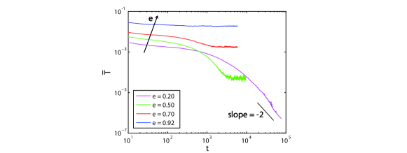
Figure 3: Time evolution of the mean granular temperature for different values of the coefficient of restitution when $\bar{\nu}=0.45$ and $\psi=\pi/5$.

The time at which the steady state is reached increases when the coefficient of restitution decreases (e.g., see Fig. 3 for the case $\psi=\pi/5$). For sufficiently small coefficients of restitution (case $e=0.2$ in Fig. 3), the mean granular temperature continues to decrease, without reaching a steady state. The slope of the curve approaches the value -2 that characterizes the Homogeneous Cooling State (HCS),Goldhirsch (2003) where the rate of change of the granular temperature in the balance of fluctuating energy is only due to the collisional dissipation and the granular temperature obeys the Haff’s law, Haff (1983) $T\propto\left(1+t\right)^{-2}$. We will discuss in Sec. IV this finding.
Once the steady state is reached, measurements are averaged in time, over at least 2000 time steps, and over the lengths of the domain along the $x$ and $z$ directions, using 20 horizontal slices. Given that the averaging is sensitive to the amplitude of the spatial discretization,Weinhart et al. (2013) we chose a number of slices that does not affect the results. Example of profiles of $\nu$, $u$, $T$ and $u^{\prime}$ are plotted in Fig. 4 for $\psi=\pi/5$ and $e=0.80$, when 20 or 40 horizontal slices are employed. Also shown are the results of the numerical integration of the EKT described in Sec. IV. The velocity profile has a characteristic S-shape, in agreement with recent physical experiments performed on disks.Miller et al. (ress) Also, the profile of the shear rate very much resembles the experimental findings. The volume fraction increases and the granular temperature decreases with distance from the walls. The core of the flow is dense, i.e., the volume fraction is larger than 0.49, and there the molecular chaos assumption breaks down. All those features are well captured by kinetic theory.

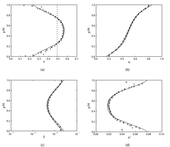
Figure 4: Profiles of $\nu$, $u$, $T$ and $u^{\prime}$ obtained from SS-DEM simulation when $H=18$, $\bar{\nu}=0.45$, $\psi=\pi/5$ and $e=0.80$, when the domain along the $y$-direction is divided into 20 (open circles) and 40 (crosses) slices to perform the averaging. The solid lines are the results of EKT when Eq. (18) and Eq. (6) are employed. The dashed line in (a) is the value of the volume fraction at the freezing point, $\nu=0.49$.

IV Results and comparisons

We first use the numerical results obtained on simple shear flows of frictionless spheres by Mitarai and Nakanishi (2007) and Chialvo and Sundaresan (2013) to derive the expression of the radial distribution function $g_{0}$. Mitarai and Nakanishi (2007) performed ED simulations of inelastic hard spheres, whereas Chialvo and Sundaresan (2013) used a SS-DEM code with a linear spring-dashpot model. In both works, the Lees-EdwardsLees and Edwards (1972) boundary conditions were implemented in the shearing direction, in order to allow for the system to remain homogeneous during the shearing. From the constitutive relation for the pressure (2) and the expressions of Tab. 1,

$$g_{0}=\dfrac{1}{2\nu(1+e)}\left(\dfrac{p}{\nu T}-1\right),$$ (15)

so that the radial distribution function can be obtained from the numerical values of pressure, volume fraction and granular temperature. For small volume fractions, $g_{0}$ obeys the Carnahan and Starling’s expression,Carnahan and Starling (1969)

$$g_{0,{\mbox{\scriptsize cs}}}=\dfrac{2-\nu}{2\left(1-\nu\right)^{3}},$$ (16)

whereas Torquato’sTorquato (1995) proposed, on the basis of numerical results on elastic particles,

$$g_{0,{\mbox{\scriptsize t}}}=\begin{cases}\begin{array}[]{lr}g_{0,{\mbox{\scriptsize cs}}}&\mbox{ if }\nu<0.49,\\ \dfrac{\left(2-0.49\right)}{2\left(1-0.49\right)^{3}}\dfrac{\left(\nu_{\mbox{\scriptsize rcp}}-0.49\right)}{\left(\nu_{\mbox{\scriptsize rcp}}-\nu\right)}&\mbox{ otherwise.}\end{array}\end{cases}$$ (17)

with $\nu_{\mbox{\scriptsize rcp}}=0.636$ the value of volume fraction at random close packing. Fig. 5 shows the radial distribution function obtained from the numerical simulations of Mitarai and Nakanishi (2007) and Chialvo and Sundaresan (2013) on simple shear flows and the present SS-DEM simulations of bounded shear flows. Eq. (17) fits well the numerical results in the case of nearly elastic particles (Fig. 5a), while underestimates the data for dense flows of particles when $e\leq 0.95$ (Fig. 5b). In the latter case, we propose to use the following expression:

$$g_{0}=fg_{0,{\mbox{\scriptsize cs}}}+\left(1-f\right)\dfrac{2}{\nu_{\mbox{\scriptsize rcp}}-\nu},$$ (18)

where $f$ is a function of the volume fraction which makes $g_{0}$ equal to the Carnahan and Starling’s expression when the volume fraction is less than a limit value, $\nu_{\mbox{\scriptsize m}}$,

$$f=\begin{cases}\begin{array}[]{lr}1&\mbox{ if }\nu<\nu_{\mbox{\scriptsize m}},\\ \dfrac{\nu^{2}-2\nu_{\mbox{\scriptsize m}}\nu+\nu_{\mbox{\scriptsize rcp}}\left(2\nu_{\mbox{\scriptsize m}}-\nu_{\mbox{\scriptsize rcp}}\right)}{2\nu_{\mbox{\scriptsize rcp}}\nu_{\mbox{\scriptsize m}}-\nu_{\mbox{\scriptsize m}}^{2}-\nu_{\mbox{\scriptsize rcp}}^{2}}&\mbox{ otherwise.}\end{array}\end{cases}$$ (19)

We take $\nu_{\mbox{\scriptsize m}}=0.4$; the quadratic expression for $f$ when $\nu\geq\nu_{\mbox{\scriptsize m}}$ ensures that the first derivative of $g_{0}$ is continuous, facilitating the numerical integration of the equations.

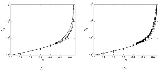
Figure 5: Numerical (symbols) radial distribution function (after Mitarai and Nakanishi (2007), Chialvo and Sundaresan (2013) and present SS-DEM simulations) as a function of the volume fraction for: (a) $e=0.98$ and 0.99; (b) $0.5\leq e\leq 0.95$. Also shown are Eq. (18) (solid line) and the expressions of Carnahan and Starling (dot-dashed line) and Torquato (dotted line).

In simple shear flows, the divergence of the flux of fluctuating energy in Eq. (1) can be neglected, and the correlation length reduces to:

$$L=\dfrac{f_{3}T^{3/2}}{su^{\prime}}.$$ (20)

In Fig. 6 we plot the quantity $f_{3}T^{3/2}/\left(su^{\prime}\right)$ as a function of the volume fraction, where $s$ and $T$ are those measured by Chialvo and Sundaresan (2013) in their SS-DEM simulations, while $f_{3}$ is evaluated from the expression of Tab. 1, using Eq. (18) and the measured values of the volume fraction. There, the lines represent the theoretical expression of the correlation length, which, in simple shear flows, using Eqs. (3),(6) and (20), is

$$L=\max\left(1,\dfrac{f_{2}^{1/3}}{f_{3}^{1/3}}{L^{*}}^{2/3}\right).$$ (21)

The agreement between the numerical data and the theoretical expression of $L$ is remarkable. In Fig. 6(b) we also plot, for comparison, the correlation length obtained from the modification of the kinetic theory suggested by Chialvo and Sundaresan (2013) when $e=0.7$.

In simple shear flows, an algebraic relation between the shear rate and the granular temperature exists,

$$\dfrac{T}{{u^{\prime}}^{2}}=\dfrac{f_{2}}{f_{3}}L.$$ (22)

Substituting Eq. (22) in Eq. (2) and Eq. (3) leads to the following expressions for the pressure,

$$p=f_{1}\dfrac{f_{2}}{f_{3}}L{u^{\prime}}^{2},$$ (23)

the shear stress

$$s=\left(\dfrac{f_{2}^{3}}{f_{3}}L\right)^{1/2}{u^{\prime}}^{2},$$ (24)

and the stress ratio

$$\dfrac{s}{p}=\left(\dfrac{f_{2}f_{3}}{f_{1}^{2}L}\right)^{1/2}.$$ (25)

The quantities $T/{u^{\prime}}^{2}$, $p/{u^{\prime}}^{2}$ and $s/p$, obtained from the numerical simulations of Mitarai and Nakanishi (2007) and Chialvo and Sundaresan (2013), are shown in Figs. 7(a), 8(a) and 9(a), respectively, for different values of the coefficient of restitution. The lines represent Eqs. (22), (23) and (25) with the radial distribution function given by Eq. (18) and the correlation length given by Eq. (21). In Figs. 7(b), 8(b) and 9(b) we also plot, for the case $e=0.7$, the predictions of the present theory if the breaking of the molecular chaos is not accounted for (i.e., $L=1$) and the predictions from the theory of Chialvo and Sundaresan (2013).

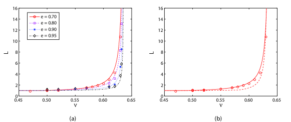
Figure 6: (a) Numerical (symbols, after Mitarai and Nakanishi (2007) and Chialvo and Sundaresan (2013)) and theoretical (lines, Eq. (20)) correlation length as a function of the volume fraction, for different values of the coefficient of restitution: $e=0.70$ (circles and solid line); $e=0.80$ (squares and dashed line); $e=0.90$ (stars and dotted line); $e=0.95$ (diamonds and dot-dashed line). (b) Same as in Fig. 6(a) for the case $e=0.7$. The dashed line represents the theory of Chialvo and Sundaresan (2013).

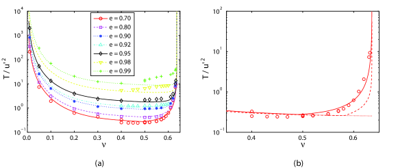
Figure 7: (a) Numerical (symbols, after Mitarai and Nakanishi (2007) and Chialvo and Sundaresan (2013)) and theoretical (lines, Eq. (22)) ratio of granular temperature to the square of the shear rate as a function of the volume fraction, for different values of the coefficient of restitution. (b) Same as in Fig. 7(a) for the case $e=0.7$. The dotted line represents the present theory when $L=1$, while the dashed line the theory of Chialvo and Sundaresan (2013).

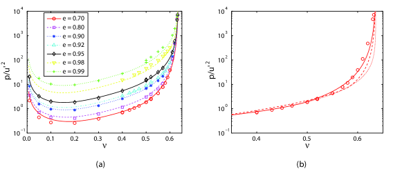
Figure 8: (a) Numerical (symbols, after Mitarai and Nakanishi (2007) and Chialvo and Sundaresan (2013)) and theoretical (lines, Eq. (23)) ratio of pressure to the square of the shear rate as a function of the volume fraction, for different values of the coefficient of restitution. (b) Same as in Fig. 8(a) for the case $e=0.7$. The dotted line represents the present theory when $L=1$, while the dashed line the theory of Chialvo and Sundaresan (2013).

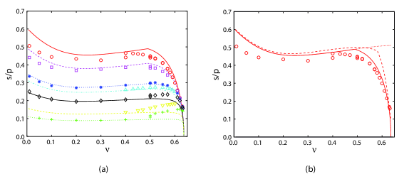
Figure 9: (a) Numerical (symbols, after Mitarai and Nakanishi (2007) and Chialvo and Sundaresan (2013)) and theoretical (lines, Eq. (25)) ratio of shear stress to the pressure as a function of the volume fraction, for different values of the coefficient of restitution. (b) Same as in Fig. 9(a) for the case $e=0.7$. The dotted line represents the present theory when $L=1$, while the dashed line the theory of Chialvo and Sundaresan (2013).

Except for large coefficients of restitution ($e>0.95$), the granular temperature, the pressure and the stress ratio are well predicted by kinetic theory in the entire range of volume fraction, if the expressions (18) for $g_{0}$ and (21) for $L$ are adopted. Replacing Eq. (18) with Eq. (17) would allow a good fitting also for the case of nearly elastic particles ($e>0.95$).

Finally, Figs. 10(a) and 10(b) depict, respectively, the quantity $p/T$ and $s/\left(T^{1/2}u^{\prime}\right)$ as functions of the volume fraction, where $p$, $T$, $s$ and $u^{\prime}$ are those measured by Mitarai and Nakanishi (2007) and Chialvo and Sundaresan (2013), when $e=0.70$, together with the theoretical expressions of $f_{1}$ and $f_{2}$ of Tab. 1, with $g_{0}$ given by Eq. (18). Also the data obtained from the present SS-DEM simulations on bounded shear granular flows (with $e=0.70$ and $\psi=\pi/5$) are shown. All the numerical data collapse, independently of the simulation method and the flow configuration, and are in very good agreement with the theoretical curves. Similar agreement is obtained for other values of the coefficient of restitution. In particular, Fig. 10(b) indicates that there is no need to modify the constitutive relation of the shear stress of kinetic theory, at least if the particles are sufficiently inelastic. Berzi (2014) We now compare the results of the numerical integration of Eqs. (8)-(11), with the SS-DEM simulations in terms of profiles of volume fraction, velocity and granular temperature, distinguishing between small and large bumpiness.

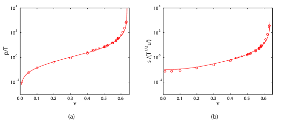
Figure 10: Numerical (after Mitarai and Nakanishi (2007), crosses; Chialvo and Sundaresan (2013), circles; present SS-DEM simulations, squares) quantities $p/T$ (a) and $s/\left(T^{1/2}u^{\prime}\right)$ (b) as functions of the volume fraction for $e=0.70$, compared with the theoretical expression of $f_{1}$ and $f_{2}$ of Tab. 1 (lines).

IV.1 Small bumpiness

Figs. 11(a), 12(a) and 13(a) show that, at small bumpiness ($\psi=\pi/5$), and using the boundary conditions of Richman (1988), EKT only qualitatively reproduces the SS-DEM results, when $\bar{\nu}=0.45$ as in the simulations. Those boundary conditions were developed for nearly elastic particles. Actually, the slip velocity and the volume fraction are underestimated, and the granular temperature is strongly overestimated when the coefficient of restitution is far from unity. In general, the SS-DEM simulations show that the volume fraction increases with the distance from the wall (Fig. 11a), and the walls are always “hotter” than the interior (Fig. 13a), i.e., the boundaries are energetic (the fluctuating energy flux is directed towards the interior of the flow); for very inelastic particles, a dense core surrounded by two more dilute layers appear (Fig. 11a). Also, the slip velocity increases as the coefficient of restitution decreases: for $e=0.50$ the granular material roughly moves as a plug (Fig. 12a). Fig. 14(a) depicts the value of the slip velocity $u_{w}$ as a function of the coefficient of restitution. For $e=0.5$, the slip velocity approaches the value 0.5, for which there is a condition of perfect slip at the walls: in that case, the particles do not touch the walls, so that no exchange of energy with the boundaries is possible. This is the reason why, for $e$ lower than 0.5, the energy initially put into the system is entirely dissipated in collisions and the evolution of the mean granular temperature obeys the Haff’s law (Fig. 3). Fig. 14(b) shows the ratio of the quantity $u_{w}p/\left(T_{0}^{1/2}s\right)$ obtained from the SS-DEM simulations to the coefficient $h$ obtained from Eq. (13) using $\psi=\pi/5$ and the numerical values of the volume fraction at the walls. The boundary condition on the slip velocity of Richman (1988) must be corrected in order to reproduce the measurements. On the basis of best fitting, we propose to use

$$\frac{u_{w}}{T_{0}^{1/2}s/p}=h\exp(7.3-8.6e).$$ (26)

which represents the solid line in Fig. 14(b). If we employ Eq. (26) instead of Eq. (12) as a boundary condition, when numerically integrating the equations of EKT, the agreement with the numerical simulations is remarkable even in the case of very inelastic particles (Figs. 11b, 12b and 13b). We expect the numerical coefficients in Eq. (26) to depend on the bumpiness and, perhaps, the particle stiffness. We postpone to future works a systematic investigation on the role of those quantities in determining the correction to the slip velocity.

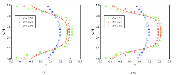
Figure 11: Profile of volume fraction obtained from the present SS-DEM simulations (symbols) for $\psi=\pi/5$, $\bar{\nu}=0.45$ and various coefficients of restitution. The data are compared with the numerical integration of Eqs. (8)-(11) for $e=0.50$ (dashed line), $e=0.70$ (solid line) and $e=0.92$ (dot-dashed line) when: (a) the boundary condition on the slip velocity is Eq. (12); (b) the boundary condition on the slip velocity is Eq. (26).

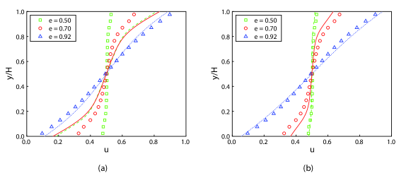
Figure 12: Same as in Fig. 11, but for the profile of velocity.

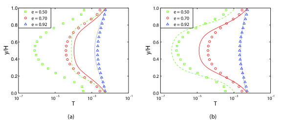
Figure 13: Same as in Fig. 11, but for the profile of granular temperature.

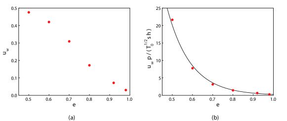
Figure 14: (a) Slip velocity as a function of the coefficient of restitution obtained from the present SS-DEM simulation when $\psi=\pi/5$. (b) Correction for the theoretical expression of the coefficient $h$ given in Eq. (13) obtained from the present SS-DEM simulations. The solid line represents Eq. (26).

IV.2 Large bumpiness

The SS-DEM simulations indicate (Figs. 15, 16 and 17) that, at large bumpiness ($\psi=\pi/3$), the volume fraction and the granular temperature are rather uniform, and the velocity profile is linearly distributed with zero slip velocity (Fig. 16), as for simple shear flows. Predictions of EKT in the case $\psi=\pi/3$ when the boundary conditions Eqs. (12) and (14) are employed strongly disagree with the SS-DEM results (Figs. 15a, 16a and 17a). Visual observation of the particle motion suggests that for large enough bumpiness, some of the flowing particles get stuck in the gaps between the particles glued at the walls; those trapped particles contribute then to create a “disordered” bumpy wall, similar to that employed in the numerical simulations of Silbert et al. (2001), which is far less energetic than the “ordered” bumpy wall of Richman (1988). In the cases $e=0.70$ and 0.92, the walls are even slightly colder than the interior (Fig. 17a), i.e., the boundaries are dissipative (the fluctuating energy flux is directed towards the walls). If we use the mean volume fraction obtained by averaging the SS-DEM profiles and $u_{w}=Q_{w}=0$ instead of Eqs. (12) and (14), i.e., we assume that the boundaries are neutral (they do not furnish nor subtract fluctuating energy), as boundary conditions, the numerical integration of EKT, which coincides with the analytical solution of simple shear flows, provides a fairly good agreement with the SS-DEM simulations (Figs. 15b, 16b and 17b). To check our intuition about the particles being trapped at the walls, we have also performed SS-DEM simulations, with $e=0.7$, when random conformations of particles are glued at the walls (the details for the generation of this kind of boundaries are given in Silbert et al. (2001)). The distribution of the volume fraction (and of the other quantities, not shown here for sake of brevity) is very similar to the case $\psi=\pi/3$ (Fig. 18a). The mean volume fraction is different in the two cases, because the space accessible to the flowing particles, whose number is constant and equal to 3132, is different. Also, the fact that the mean volume fraction measured in the SS-DEM simulatons $\bar{\nu}_{{\mbox{\scriptsize DEM}}}$ is, in general, less than the theoretical value 0.44, that would characaterize the $\psi=\pi/3$ case when $N=3132$, is an indication of particle trapping. Indeed, a rough estimate of the thickness $\Delta$ of this trapped particle layer is

$$\Delta=\frac{N}{2L_{x}L_{z}}\left(1-\frac{\bar{\nu}_{{\mbox{\scriptsize DEM}}}}{0.44}\right).$$ (27)

Fig. 18(b) shows that $\Delta$ goes to zero as $e$ approaches one. Also, the thickness $\Delta$ saturates to a constant value for coefficients of restitution lower than 0.7. Once again, we postpone to future works the generalization of these findings to other values of the bumpiness and the particle stiffness.
Finally, Fig. 19 shows the influence of the coefficient of restitution on the stress ratio, $s/p$. Contrary to results reported for 2D plane shear flows of frictional grains submitted to imposed pressure,da Cruz et al. (2005) the coefficient of restitution strongly affects the stress ratio. In the range $0.50\leq e\leq 0.98$, the stress ratio obtained from the present SS-DEM simulations is a decreasing function of the coefficient of restitution for large bumpiness ($\psi=\pi/3$); while $s/p$ has a maximum around $e=0.80$ for small bumpiness ($\psi=\pi/5$). The predictions of EKT when Eqs. (26) and (14) are employed as boundary conditions for $\psi=\pi/5$, and $u_{w}=Q_{w}=0$ for $\psi=\pi/3$ are, once again, in a fairly good agreement with the simulations. The drop in the stress ratio for small bumpiness and coefficients of restitution less than 0.8 is due to the already mentioned increasing of the slip velocity, with the corresponding approaching to the Homogeneous Cooling State, in which the shear stress, and consequently the stress ratio, vanishes.

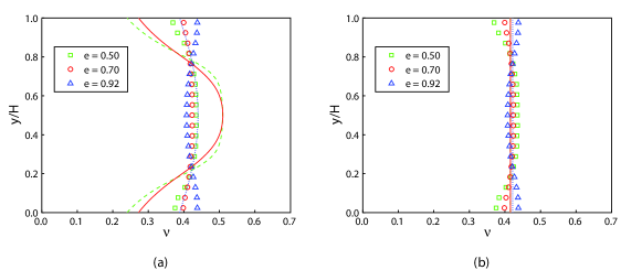
Figure 15: Profile of volume fraction obtained from the present SS-DEM simulations (symbols) for $\psi=\pi/3$ and various coefficients of restitution. The data are compared with the numerical integration of Eqs. (8)-(11) for $e=0.50$ (dashed line), $e=0.70$ (solid line) and $e=0.92$ (dot-dashed line) when: (a) the boundary conditions are Eq. (12) and Eq. (14); (b) the boundary conditions are $u_{w}=Q_{w}=0$. In both cases, the mean volume fraction is that measured in the simulations.

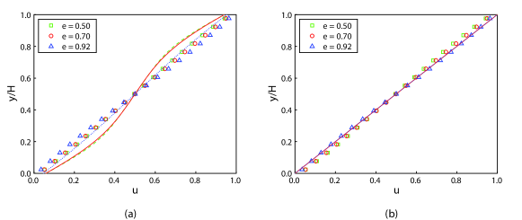
Figure 16: Same as in Fig. 15, but for the profile of velocity.

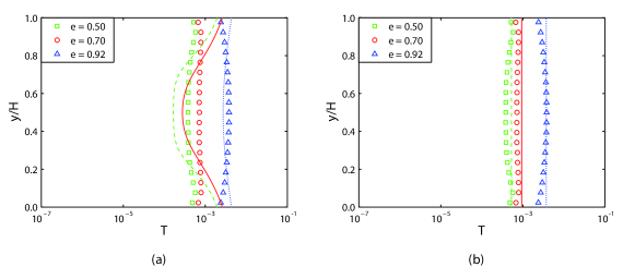
Figure 17: Same as in Fig. 15, but for the profile of granular temperature.

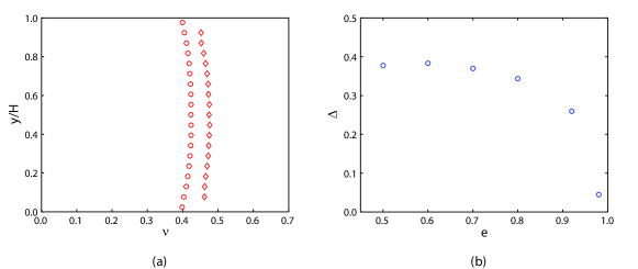
Figure 18: (a) Profile of volume fraction obtained from the present SS-DEM simulations with ordered ($\psi=\pi/3$, circles) and disordered (diamonds) bumpy walls, when $e=0.7$ and $N=3132$. (b) Thickness of the trapped particle layer as a function of the coefficient of restitution when $\psi=\pi/3$.

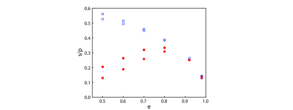
Figure 19: Stress ratio $s/p$ as a function of the coefficient of restitution obtained from the SS-DEM simulations when $\psi=\pi/5$ (filled circles) and $\psi=\pi/3$ (open circles), and from the numerical integration of Eqs. (8)-(11) with the proposed modifications of the boundary conditions ($\psi=\pi/5$, filled squares; and $\psi=\pi/3$, open squares).

V Conclusions

In this paper, the Extended Kinetic Theory is numerically solved for the shear flows of identical, frictionless particles bounded between two parallel, bumpy planes, at constant volume (plane shear flow). The bumpiness is due to spheres identical to those of the flow, glued at the walls in a regularly spaced, hexagonal array. The numerical solutions are compared with 3D SS-DEM simulations, and the roles of the coefficient of restitution and the bumpiness of the boundaries are investigated. We propose an expression for the radial distribution function to be used when $e\leq 0.95$ which coincides with the Carnahan and Starling’sCarnahan and Starling (1969) at small volume fraction, and diverges as the volume fraction approaches the shear rigidity as the Torquato’s,Torquato (1995) but, unlike the latter, its derivative is continuous in the entire range of volume fraction. We have shown that the proposed expression fits well the results of ED and SS-DEM simulations of simple shear flows. Also, we adopt a recently suggested expression for the correlation length in the dissipation rate of fluctuating energy, which depends only on the coefficient of restitution. At small bumpiness, the SS-DEM simulations show that the volume fraction increases with the distance from the wall, for every value of the coefficient of restitution, and the wall is always “hotter” than the interior. The slip velocity at the boundaries decreases with the elasticity of the particles, and, for coefficients of restitution less than 0.5, the slip is perfect: the boundaries do not touch the flowing particles, so that the system evolves accordingly to the Homogeneous Cooling State (it is not possible to obtain a steady shear flow). Also, the measured stress ratio is a non monotonic function of the coefficient of restitution, and reaches a maximum for $e=0.80$. The results of the numerical integration of EKT agree well with the simulations, if a correction to the expression of the slip velocity depending on the coefficient of restitution is introduced in the boundary conditions derived for nearly elastic particles by Richman (1988). At large bumpiness, the SS-DEM simulations show nearly uniform profiles of volume fraction and granular temperature, and linear distributions of the velocity field, as for simple shear flows. This is due to the fact that, when the gaps between the spheres glued at the walls are large enough, some of the flowing particles get stuck, making the bumpy wall more “disordered”, and, then, more dissipative than expected. Even in the case of large bumpiness, EKT is able to reproduce the simulation results, if both the slip velocity and the fluctuating energy flux at the walls are taken to be zero.
Summarizing, we have shown that Extended Kinetic Theory has the capability of quantitatively reproducing the flow of frictionless spheres in the entire range of volume fraction for which the collisions can be considered nearly instantaneous and random (i.e., the entire fluid-like regime of granular flows). Tests of proposed extensions to EKT to deal with friction, non-instantaneous collisions and enduring contacts will be the subject of future works.

References

- Jenkins and Savage (1983) J. Jenkins and S. Savage, “A theory for the rapid flow of identical, smooth, nearly elastic, spherical particles,” Journal of Fluid Mechanics 130, 187–202 (1983).
- Lun (1991) C. Lun, “Kinetic theory for granular flow of dense, slightly inelastic, slightly rough spheres,” Journal of Fluid Mechanics 233, 539–559 (1991).
- Garzó and Dufty (1999) V. Garzó and J. W. Dufty, “Dense fluid transport for inelastic hard spheres,” Physical Review E 59, 5895–5911 (1999).
- Goldhirsch (2003) I. Goldhirsch, “Rapid granular flows,” Annual Review of Fluid Mechanics 35, 267–293 (2003).
- Campbell (2002) C. Campbell, “Granular shear flows at the elastic limit,” Journal of Fluid Mechanics 465, 261–291 (2002).
- Mitarai and Nakanishi (2007) N. Mitarai and H. Nakanishi, “Velocity correlations in the dense granular shear flows: Effects on energy dissipation and normal stress,” Physical Review E 75, 031305–031313 (2007).
- Kumaran (2009) V. Kumaran, “Dynamic of dense sheared granular flows. Part 1. Structure and diffusion,” Journal of Fluid Mechanics 632, 109–144 (2009).
- Majmudar and Behringer (2005) T. Majmudar and R. Behringer, “Contact force measurements and stress-induced anisotropy in granular materials,” Nature 435, 1079–1082 (2005).
- da Cruz et al. (2005) F. da Cruz, S. Emam, M. Prochnow, J.-N. Roux, and F. Chevoir, “Rheophysics of dense granular materials: Discrete simulation of plane shear flows,” Physical Review E 72, 021309–021326 (2005).
- Jenkins (2006) J. Jenkins, “Dense shearing flows of inelastic disks,” Physics of Fluids 18, 103307–103315 (2006).
- Jenkins (2007) J. Jenkins, “Dense inclined flows of inelastic spheres,” Granular Matter 10, 47–52 (2007).
- Johnson and Jackson (1987) P. Johnson and R. Jackson, “Frictional-collisional constitutive relations for granular materials, with application to plane shearing,” Journal of Fluid Mechanics 176, 67–93 (1987).
- Johnson and Jackson (1990) P. Johnson and R. Jackson, “Frictional-collisional equations of motion for particulate flows and their application to chutes,” Journal of Fluid Mechanics 210, 501–535 (1990).
- Louge (2003) M. Louge, “Model for dense granular flows down bumpy inclines,” Physical Review E 67, 061303 (2003).
- Berzi, di Prisco, and Vescovi (2011) D. Berzi, C. di Prisco, and D. Vescovi, “Constitutive relations for steady, dense granular flows,” Physical Review E 84, 031301–031306 (2011).
- Vescovi, di Prisco, and Berzi (2013) D. Vescovi, C. di Prisco, and D. Berzi, “From solid to granular gases: the steady state for granular materials,” International Journal for Numerical and Analytical Methods in Geomechanics 37, 2937–2951 (2013).
- Lees and Edwards (1972) A. Lees and S. F. Edwards, “The computer study of transport processes under extreme conditions,” Journal of Physics C: Solid State Physics 5, 1921–1929 (1972).
- Ji and Shen (2006) S. Ji and H. Shen, “Characteristics of temporalspatial parameters in quasisolid-fluid phase transition of granular materials,” Chinese Science Bulletin 51, 646–654 (2006).
- Chialvo and Sundaresan (2013) S. Chialvo and S. Sundaresan, “A modified kinetic theory for frictional granular flows in dense and dilute regimes,” Physics of Fluids 25, 070603 (2013).
- Shojaaee et al. (2012) Z. Shojaaee, J.-N. Roux, F. Chevoir, and D. Wolf, “Shear flow of dense granular materials near smooth walls. I. Shear localization and constitutive laws in the boundary region,” Physical Review E 86, 1–12 (2012).
- Karion and Hunt (2000) A. Karion and M. Hunt, “Wall stresses in granular Couette flows of mono-sized particles and binary mixtures,” Powder Technology 109, 145–163 (2000).
- Liu and Rosato (2005) J. Liu and A. Rosato, “General features of granular Couette flow and intruder dynamics,” Journal of Physics: Condensed Matter 17, S2609–S2622 (2005).
- Xu, Louge, and Reeves (2003) H. Xu, M. Louge, and A. Reeves, “Solutions of the kinetic theory for bounded collisional granular flows,” Continuum Mechanics and Thermodynamics 15, 321–349 (2003).
- Orlando and Shen (2012) A. Orlando and H. Shen, “Effect of particle size and boundary conditions on the shear stress in an annular shear cell,” Granular Matter 14, 423–431 (2012).
- Miller et al. (ress) T. Miller, P. Rognon, B. Metzger, and I. Einav, “Eddy viscosity in dense granular flows,” Physical Review Letters (2013 in press).
- Berzi (2014) D. Berzi, “Extended kinetic theory applied to dense, granular, simple shear flows.” Acta Mechanica (published online2014), 10.1007/s00707-014-1125-1.
- Richman (1988) M. Richman, “Boundary conditions based on a modified maxwellian velocity distribution function for flows of identical, smooth, nearly elastic spheres.” Acta Mechanica 75, 227–240 (1988).
- Carnahan and Starling (1969) N. Carnahan and K. Starling, “Equation of state for nonattracting rigid spheres,” Journal of Chemical Physics 51, 635–636 (1969).
- Torquato (1995) S. Torquato, “Nearest-neighbor statistics for packing of hard spheres and disks,” Physical Review E 51, 3170–3182 (1995).
- Jenkins and Berzi (2010) J. Jenkins and D. Berzi, “Dense inclined flows of inelastic spheres: tests of an extension of kinetic theory,” Granular Matter 12, 151–158 (2010).
- Berzi and Jenkins (2011) D. Berzi and J. Jenkins, “Surface flows of inelastic spheres,” Physics of Fluids 23, 013303–013310 (2011).
- Jenkins and Berzi (2012) J. Jenkins and D. Berzi, “Kinetic theory applied to inclined flows,” Granular Matter 14, 79–84 (2012).
- Brodu, Richard, and Delannay (2013) N. Brodu, P. Richard, and R. Delannay, “Shallow granular flows down flat frictional channels: Steady flows and longitudinal vortices,” Phys. Rev. E 87, 022202 (2013).
- Silbert et al. (2001) L. Silbert, D. Ertas, G. Grest, T. Halsey, D. Levine, and S. Plimpton, “Granular flow down an inclined plane: Bagnold scaling and rheology,” Physical Review E 64, 051302–051318 (2001).
- Taberlet, Richard, and Delannay (2008) N. Taberlet, P. Richard, and R. Delannay, “The effect of sidewall friction on dense granular flows,” Computers & Mathematics with Applications 55, 230 – 234 (2008).
- Taberlet and Richard (2006) N. Taberlet and P. Richard, “Diffusion of a granular pulse in a rotating drum,” Phys. Rev. E 73, 041301 (2006).
- Rycroft, Orpe, and Kudrolli (2009) C. H. Rycroft, A. V. Orpe, and A. Kudrolli, “Physical test of a particle simulation model in a sheared granular system,” Phys. Rev. E 80, 031305 (2009).
- Majmudar et al. (2007) T. S. Majmudar, M. Sperl, S. Luding, and R. P. Behringer, “Jamming transition in granular systems,” Physical Review Letters 98, 058001 (2007).
- Hirshfeld and Rapaport (2001) D. Hirshfeld and D. Rapaport, “Granular flow from a silo: Discrete-particle simulations in three dimensions,” The European Physical Journal E: Soft Matter and Biological Physics 4, 193–199 (2001).
- Richard, McNamara, and Tankeo (2012) P. Richard, S. McNamara, and M. Tankeo, “Relevance of numerical simulations to booming sand,” Phys. Rev. E 85, 010301 (2012).
- Richard et al. (2008) P. Richard, A. Valance, J.-F. Métayer, P. Sanchez, J. Crassous, M. Louge, and R. Delannay, “Rheology of confined granular flows: Scale invariance, glass transition, and friction weakening,” Physical Review Letters 101, 248002 (2008).
- Luding (2008) S. Luding, “Introduction to discrete element methods: Basics of contact force models and how to perform the micro-macro transition to continuum theory,” European Journal of Environmental and Civil Engineering - EJECE 12 12, 785–826 (2008).
- Otsuki, Hayakawa, and Luding (2010) M. Otsuki, H. Hayakawa, and S. Luding, “Behavior of pressure and viscosity at high densities for two-dimensional hard and soft granular materials,” Progress of Theoretical Physics Supplement 184, 110–133 (2010).
- Haff (1983) P. Haff, “Grain flow as a fluid-mechanical phenomenon,” Journal of Fluid Mechanics 134, 401–430 (1983).
- Weinhart et al. (2013) T. Weinhart, R. Hartkamp, A. Thornton, and S. Luding, “Coarse-grained local and objective continuum description of 3D granular flows down an inclined surface,” Physics of Fluids 25, 070605 (2013).