The Surface Laplacian Technique in EEG: Theory and Methods

Abstract

This paper reviews the method of surface Laplacian differentiation to study EEG. We focus on topics that are helpful for a clear understanding of the underlying concepts and its efficient implementation, which is especially important for EEG researchers unfamiliar with the technique. The popular methods of finite difference and splines are reviewed in detail. The former has the advantage of simplicity and low computational cost, but its estimates are prone to a variety of errors due to discretization. The latter eliminates all issues related to discretization and incorporates a regularization mechanism to reduce spatial noise, but at the cost of increasing mathematical and computational complexity. These and several others issues deserving further development are highlighted, some of which we address to the extent possible. Here we develop a set of discrete approximations for Laplacian estimates at peripheral electrodes and a possible solution to the problem of multiple-frame regularization. We also provide the mathematical details of finite difference approximations that are missing in the literature, and discuss the problem of computational performance, which is particularly important in the context of EEG splines where data sets can be very large. Along this line, the matrix representation of the surface Laplacian operator is carefully discussed and some figures are given illustrating the advantages of this approach. In the final remarks, we briefly sketch a possible way to incorporate finite-size electrodes into Laplacian estimates that could guide further developments.

1 Introduction

The surface Laplacian technique is a powerful method to study EEG. It emerged back in the 1970’s, from the seminal works of Nicholson (1973), Freeman and Nicholson (1975), Nicholson and Freeman (1975), and Hjorth (1975). These works were followed by efforts to develop better computational methods (see Gevins, 1988, 1989; Gevins et al., 1990; Perrin et al., 1989; Law et al., 1993a; Yao, 2002; Carvalhaes and Suppes, 2011) as well as attempts to combine the surface Laplacian with other methods (Kayser and Tenke, 2006b, a; Carvalhaes et al., 2009), making the technique increasingly popular among EEG researchers. For instance, modern applications include studies on generators of event-related potentials (Kayser and Tenke, 2006b, a), quantitative EEG (Tenke et al., 2011), spectral coherence (Srinivasan et al., 2007; Winter et al., 2007), event-related synchronization/desynchronization (Del Percio et al., 2007), phase-lock synchronization (Doesburg et al., 2008), estimation of cortical connectivity (Astolfi et al., 2007), high-frequency EEG Fitzgibbon et al. (2013), and brain-computer interface (Lu et al., 2013), just to mention a few.

The motivation for the use of the surface Laplacian technique is grounded on Ohm’s law. This law establishes a local relationship between the surface Laplacian of scalp potentials and the underlying flow of electric current caused by brain activity (see Appendix in Carvalhaes et al., 2014). Presumably, this local relation should improve spatial resolution, reflecting electrical activity from a more restricted cortical area than what is observed in conventional topography.

In contrast to other high-resolution techniques, such as cortical surface imaging (Nunez et al., 1994; Yao, 1996; Yao et al., 2001), the surface Laplacian has the advantage of not requiring a volume conductor model of the head or a detailed specification of neural sources, but objections to it may arise due to a combination of factors. First, there is a noticeable difficulty in understanding the technique in depth (Nunez and Westdorp, 1994). While EEG potentials can be physically understood in terms of current flow or in analogy with the gravitational potential, interpreting the surface Laplacian operation seems much less intuitive, as it involves the application of a second-order partial differential operator to a scalar potential distribution. Second, it appears surprising to many that one can actually obtain a reference-independent quantity from a signal which is seen to have been contaminated by a reference in its very origin (Nunez and Srinivasan, 2006, ch 7). Third, it is not possible to guarantee that the theoretical advantages associated to the use of the Laplacian differentiation will be preserved in the practical world of imperfect measurements and finite samples. In fact, reliable estimates of the Laplacian derivation are technically challenging, and computational methods to perform this task are still a subject of research.

The literature dedicated to provide theoretical explanations about the surface Laplacian technique is scarce, but it contains substantial and valuable information (see Nunez and Srinivasan, 2006; Tenke and Kayser, 2012). Nevertheless, there are still some gaps that, if filled, can help comprehension and permit a more intuitive view of the technique. It is the primary intention of this paper to contribute to this matter. For this purpose, Section 2 provides physical insights on the surface Laplacian technique that are often not discussed in the literature, but that are at the heart of some of the issues of interest to the EEG researcher. Section 3 focuses on the computational aspects of this technique, providing a comprehensive review of selected computational methods and their advantages and limitations. Two sections were devoted to topics that in our view deserve a more detailed discussion. In Section 3.5 we present the method of estimating the surface Laplacian derivation by means of a matrix transformation, and Section 3.6 focuses on the regularization problem of smoothing splines that significantly affects surface Laplacian estimates.

2 An Overview of the Physics of EEG

In this Section we discuss the main theoretical ideas behind the use of the surface Laplacian. Our goal here is to introduce some concepts from the physics of EEG that are often unfamiliar to the EEG researcher, and that have direct relevance to the surface Laplacian technique. We do not attempt to reproduce the main arguments about the relationship between the surface Laplacian and the dura-surface potential, nor with the Current Source Density (CSD), which are found, for example, in Nunez and Srinivasan (2006) and Tenke and Kayser (2012). Instead we focus on the more fundamental aspects that are often overlooked.

2.1 Physical interpretation of the surface Laplacian

To better understand the physical meaning of the surface Laplacian, it is instructive to start with the volume Laplacian, or simply Laplacian, and its relationship to the quasi-static electric field and potential. Here our treatment is very standard, and can be found in more details in any textbook on electricity and magnetism, such as Jackson (1999) or Schey (2004), and the reader interested in more detail is referred to them. Our discussion will focus only on aspects that are directly relevant to EEG.

When we talk about scalp EEG, we are always referring to the potential with respect to some reference electrode. But, from a physics point of view, the electric field is more fundamental than the potential. To see this, let us recall that the field has a measurable effect: for a particle of charge $q$, the field $\mathbf{E}(\mathbf{r})$ at the position $\mathbf{r}$ is operationally defined by the ratio between the electric force $\mathbf{F}_{E}$ acting on the charge at $\mathbf{r}$ and the value of $q$. Here we use the standard notation of representing scalar quantities in italics and vectors in boldface, e.g. $q$ for the electric charge and $\mathbf{E}$ for the electric field, and we also use the symbol “$\equiv$” for an equality that arises from a definition. From this definition, the field is a quantity that measures the force per unit of charge, i.e., $\mathbf{E}$ (as a function of the position $\mathbf{r}$) is given by

$$\mathbf{E}(\mathbf{r})\equiv\frac{1}{q}\mathbf{F}_{E}(\mathbf{r}).$$ (1)

For simplicity, we are ignoring any temporal dependence of $\mathbf{E}$, but the results remains the same, for all practical purposes, in the typical range of frequencies involved in the brain electrical activity (Jackson, 1999; Nunez and Srinivasan, 2006).

Electric fields generated by point charges are described by Coulomb’s Law. A consequence of this law is that $\mathbf{E}$ is a conservative field, i.e., the line integral

$$V_{AB}=-\int_{\mathbf{r}_{A}}^{\mathbf{r}_{B}}\mathbf{E}(\mathbf{r})\cdot d\mathbf{r}$$ (2)

between two points $\mathbf{r}_{A}$ and $\mathbf{r}_{B}$ is independent of the path along which it is computed. The value $V_{AB}$ has an important physical meaning: it corresponds to the work per unit of charge necessary to be done on a charged particle when it goes through the field $\mathbf{E}$ from position $\mathbf{r}_{A}$ to $\mathbf{r}_{B}$ at a constant speed. Thus, the quantity $V_{AB}$ is not only measurable, but of practical use, as we will see later on. But also of importance is the fact that the path-independence of $V_{AB}$ implies the existence of a function $V\left(\mathbf{r}\right)$ such that

$$V_{AB}\equiv V\left(\mathbf{r}_{B}\right)-V\left(\mathbf{r}_{A}\right).$$ (3)

The function $V\left(\mathbf{r}\right)$ is called the electric potential of the field $\mathbf{E}$.

One important relationship between the electric field $\mathbf{E}$ and the potential $V$ is given by the gradient operator. The gradient of $V\left(\mathbf{r}\right)$, denoted $\mbox{Grad}\left(V\left(\mathbf{r}\right)\right)$, is defined, in Cartesian coordinates, as

$$\mbox{Grad}\left(V\left(\mathbf{r}\right)\right)=\frac{\partial V\left(\mathbf{r}\right)}{\partial x}\hat{\bm{\textbf{$\imath$}}}+\frac{\partial V\left(\mathbf{r}\right)}{\partial y}\hat{\bm{\jmath}}+\frac{\partial V\left(\mathbf{r}\right)}{\partial z}\hat{\bm{\bm{k}}},$$ (4)

where $\hat{\bm{\imath}}$, $\hat{\bm{\jmath}}$, and $\hat{\bm{k}}$ are the orthonormal basis vectors. The gradient $\mbox{Grad}\left(V\left(\mathbf{r}\right)\right)$ is the spatial derivative of $V$ at $\mathbf{r}$, and it forms a vector field with the following properties. For a unitary vector $\hat{\mathbf{u}},$ $\mbox{Grad}\left(V\left(\mathbf{r}^{\prime}\right)\right)\cdot\hat{\mathbf{u}}$ gives the rate of change of the function $V$ at point $\mathbf{r}^{\prime}$ in the direction $\mathbf{\hat{u}}$. Thus, $\mbox{Grad}\left(V\left(\mathbf{r}^{\prime}\right)\right)$ at $\mathbf{r}^{\prime}$ is a vector, pointing at the direction where the function $V$ changes the most, whose magnitude is the rate of change. In other words, the direction perpendicular to $\mbox{Grad}\left(V\left(\mathbf{r}^{\prime}\right)\right)$ points at the direction of the isopotential lines. From this, it is possible to prove that the function $V\left(\mathbf{r}\right)$ relates to the field by the expression

$$\mathbf{E}(\mathbf{r})=-\mathrm{Grad}(V(\mathbf{r})),$$ (5)

i.e., the electric field is the negative gradient of the electric potential.

It is easy to see that $V\left(\mathbf{r}\right)$ is not uniquely defined, as any other function $V^{\prime}\left(\mathbf{r}\right)$ given by

$$V^{\prime}\left(\mathbf{r}\right)\equiv V\left(\mathbf{r}\right)-V_{0},$$ (6)

where $V_{0}$ is an arbitrary constant, also gives the same differences of potential $V_{AB}$ between positions $\mathbf{r}_{A}$ and $\mathbf{r}_{B}$, and therefore the same gradient (for instance, when we take the limit of $\Delta\mathbf{r}=\mathbf{r}_{B}-\mathbf{r}_{A}$ very small). As an example, let us consider the electric field from a point particle with charge $q$ situated at position $\mathbf{r}_{0}$, which is given by

$$\mathbf{E}\left(\mathbf{r}\right)=\frac{q}{4\pi\epsilon_{0}}\frac{\mathbf{r}-\mathbf{r}_{0}}{\left(\mathbf{r}-\mathbf{r}_{0}\right)^{3}}.$$

It is easy to show that a potential function satisfying (2) is given by

$$V(\mathbf{r})=-\frac{q}{4\pi\epsilon_{0}}\frac{1}{\left|\mathbf{r}-\mathbf{r}_{0}\right|}.$$ (7)

For another potential function $V^{\prime}$ given by $V^{\prime}(\mathbf{r})=-\frac{q}{4\pi\epsilon_{0}}\frac{1}{\left|\mathbf{r}-\mathbf{r}_{0}\right|}+V_{0},$ we see at once that its gradient is exactly the same as for $V\left(\mathbf{r}\right)$, since any constant added to $V$ would disappear when the derivative in (4) is taken. However, the potential (7) is often given in textbooks, as it has the feature that the potential is zero in infinity ($V\rightarrow 0$ when $\left|\mathbf{r}\right|\rightarrow\infty$), which corresponds to a reference in a point infinitely distant from $\mathbf{r}_{0}$.

As we mentioned above, the potential difference has practical use. For actual measurements, directly observing the electric field is very difficult, but measuring the electric work on a test particle, related to the line integral of (7) between two points $\mathbf{r}_{A}$ and $\mathbf{r}_{B}$ is not. This is done by inserting two probes (the electrodes, in the case of the EEG) at points $\mathbf{r}_{A}$ and $\mathbf{r}_{B}$, and creating a parallel circuit with high impedance, such that minimal disturbance is created in the original potential. The current appearing in this circuit is proportional to the potential difference $V(\mathbf{r}_{B})-V(\mathbf{r}_{A})$. Thus, current measurements between different points can be used in this way to construct a map of the potential function at different positions (minus a reference value $V_{0}$, which is often arbitrarily chosen such that $V(\mathbf{r}_{\mathcal{O}})=0$ at some reference point $\mathcal{O}$).

In a volume conductor, such as the brain, the electric field is a useful quantity to know, as it is related to a current density $\mathbf{j}$ given by

$$\mathbf{E}(\mathbf{r})=\rho\,\mathbf{j}(\mathbf{r}),$$ (8)

where $\rho=1/\sigma$ is the resistivity, given by the inverse of the conductivity $\sigma$. Equation (8) is sometimes referred to as the vector form of Ohm’s Law. In a conductive media with resistivity $\rho$, a map of the potential function may be used to compute the electric field $\mathbf{E}\left(\mathbf{r}\right)$ and, via equation (8), estimate current sources. Here we must emphasize that electric potentials can never be directly measured; only potential differences between two points can.

Though in this paper we are interested in the surface Laplacian, for completeness we should also mention the physical meaning of the Laplacian. Such meaning comes from Gauss’s Law, which in its differential form given by Maxwell is written as

$$\mathrm{Div}(\mathbf{E})=4\pi\rho_{Q},$$ (9)

where $\rho_{Q}$ is the charge density. Here $\mathrm{Div}\left(\mathbf{E}\right)$ is the divergence of the electric field $\mathbf{E}$. The divergence is a linear differential operator acting on $\mathbf{E}$, which in Cartesian coordinates, where the electric field is represented by $\mathbf{E}=E_{x}\hat{\bm{\imath}}+E_{y}\hat{\bm{\jmath}}+E_{z}\hat{\bm{k}}$, takes the form

$$\mbox{Div}\left(\mathbf{E}\right)=\frac{\partial E_{x}}{\partial x}+\frac{\partial E_{y}}{\partial y}+\frac{\partial E_{z}}{\partial z}.$$

The divergence of $\mathbf{E}$ can be interpreted as a local measure of the difference between how much field (technically, its flux) gets into an infinitesimal volume surrounding the point where the divergence is computed and how much of this field gets out. If the divergence is zero, the same amount of field that gets into the infinitesimal volume also gets out; if the divergence is negative, the amount of field getting in is more than getting out (sink); and if the divergence is positive, more field gets out than comes into the infinitesimal volume (source). For this reason, the divergence of $\mathbf{E}$ is a measure of sources and sinks of the field. Thus, Gauss’s law has the immediate physical interpretation that electric charges are sources of an electric field: if there are no electric charges, the divergence of the field is zero. Now, from equation (5) we have at once that

$$\mathrm{Div}(\mathbf{E})=-\mathrm{Div}(\mathrm{Grad}(V)).$$ (10)

The divergence of the gradient, $\mathrm{Div}(\mathrm{Grad}(V))$, is defined as the Laplacian of $V$, denoted by $\mbox{Lap}\left(V\right)\equiv\mathrm{Div}(\mathrm{Grad}(V))$. Because it is a second spatial derivative, the Laplacian does not have an interpretation that is as straightforward as the ones for the divergence or the gradient. Its meaning is related to the mean value of the potential around the point where it is computed. For example, imagine that $\mbox{Lap}\left(V\right)$ is positive at some point $\mathbf{r}^{\prime}$ where $V$ has a local minimum (first derivative is zero); such positive value means that for the nearby points surrounding $\mathbf{r}^{\prime}$, most of the values of $V$ are greater than $V\left(\mathbf{r}^{\prime}\right)$. So, $\mbox{Lap}\left(V\right)$ measures the mean value around the point. Be that as it may, we can also think of the Laplacian of $V$ as simply the divergence of $\mathbf{E}$. Thus, from (10) and (9) it follows that the Laplacian of the potential is proportional to the electric field sources, i.e.,

$$\mbox{Lap}\left(V\right)=-4\pi\rho_{Q}.$$ (11)

The above discussion was intended to show the connection between the field $\mathbf{E}$ to the scalar potential $V$. However, in its generality, it does not take into account some specific characteristics of the EEG. First, the EEG is measured over the scalp, which is geometrically a curved surface. Second, such measurements are not directly of the field, but are instead differences of potential associated to small currents flowing in the closed circuit formed between the two electrodes (often between a measuring and a reference electrode), the measuring device, and the current flow density in the head. In the head, such currents define a vector field consisting of currents from the brain, dura surface, bone, and scalp. This current density is proportional at each point to the electric field. But outside of the head, the EEG measuring apparatus closes the circuit and measures the small current associated with such system (despite how high the impedance is) (Metting van Rijn et al., 1990, 1991). Finally, because such measurements are on the scalp, they happen where there is a significant change in conductivity (interface scalp/air). All of those points have some consequence for the interpretations of the field and Laplacian.

Starting with the Laplacian, the most common assumption is that sources of interest to the EEG are inside the skull, and that there are no sources in the scalp itself (Nunez and Srinivasan, 2006). But if we start with this assumption, we have that, from (9),

$$\mathrm{Lap}(V)=0.$$ (12)

Using the expression for the Laplacian in Cartesian coordinates, we have

$$\frac{\partial^{2}V}{\partial x^{2}}+\frac{\partial^{2}V}{\partial y^{2}}+\frac{\partial^{2}V}{\partial z^{2}}=0.$$ (13)

Let us now choose the coordinate system such that the scalp is on the plane $x,y$ (for small areas, this is a good approximation). Then we can rewrite (13) as

$$\frac{\partial^{2}V}{\partial x^{2}}+\frac{\partial^{2}V}{\partial y^{2}}=\frac{\partial E}{\partial z},$$ (14)

where on the right hand side we used the relationship between the field and the potential. Remembering that in a conductor $\mathbf{E}=\rho\mathbf{j}$, it follows that

$$\frac{\partial^{2}V}{\partial x^{2}}+\frac{\partial^{2}V}{\partial y^{2}}=\rho\frac{\partial j_{z}}{\partial z}.$$ (15)

The left hand side of (15) is defined as the surface Laplacian of $V$,

$$\mathrm{Lap}_{S}(V)=\frac{\partial^{2}V}{\partial x^{2}}+\frac{\partial^{2}V}{\partial y^{2}},$$ (16)

and (15) shows that $\mathrm{Lap}_{S}(V)$ is related to how abruptly the normal component of the current changes in the direction perpendicular to the surface. Thus, if $\mathrm{Lap}_{S}(V)$ is nonzero, conceptually, in the absence of sources, the current change in this direction means a fanning out of the current lines, i.e., a spreading out of the currents. In the case of the scalp, this means that a nonzero $\mathrm{Lap}_{S}(V)$ corresponds to diverging (with respect to the radial direction) current lines under the scalp, which is associated to the presence of a source of currents inside the skull. Thus, we see that the surface Laplacian has a direct relationship to currents under the scalp, and it can be shown that it is related to electrical activities on the dura surface (Nunez and Srinivasan, 2006).

2.2 Properties of the surface Laplacian

Equipped with an interpretation of the surface Laplacian in terms of currents and fields, we now turn to some its important properties. Let us start with one of the main characteristics of the surface Laplacian: it is reference free. This may seem puzzling to some, as in most cases the surface Laplacian is computed from the scalp potential, which is itself a reference-dependent quantity. To understand how this is possible, it is worth examining a simple example from geometry. Imagine we have two points, $P$ and $Q$, representing the locations of two events of interest. From an observer using the coordinate system ${\cal O}$ (see Figure 1), the positions of $P$ and $Q$ are given by the (reference-dependent) vectors $\mathbf{r}_{P}$ and $\mathbf{r}_{Q}$. That the position vectors of $P$ and $Q$ are reference dependent can be seen by the simple fact that another observer using coordinates ${\cal O}^{\prime}$ describe such positions by the vectors $\mathbf{r}^{\prime}_{P}$ and $\mathbf{r}^{\prime}_{Q}$, which are clearly different from $\mathbf{r}_{P}$ and $\mathbf{r}_{Q}$. Thus, the geometrical meaning of, say, the length of the position vector $\mathbf{r}_{P}$, is not related to the event of interest only, but to a combination of such event and an arbitrary choice of reference system, making this quantity reference dependent.

However, there are many geometrically reference-free quantities, i.e., quantities that look the same for ${\cal O}$ and ${\cal O}^{\prime}$, that can be constructed from the reference-dependent positions $\mathbf{r}_{P}$ and $\mathbf{r}_{Q}$. For example, the vector connecting $P$ and $Q$ is reference-free, since it is given by $\mathbf{r}=\mathbf{r}_{P}-\mathbf{r}_{Q}=\mathbf{r}^{\prime}_{P}-\mathbf{r}^{\prime}_{Q}$. Notice that $\mathbf{r}$ has the feature of depending only on characteristics of the system of interest, $P$ and $Q$. Another important reference-free quantity is the distance $d$ between $P$ and $Q$, defined by $d^{2}=\mathbf{r}^{2}=\left(\mathbf{r}_{P}-\mathbf{r}_{Q}\right)\cdot\left(\mathbf{r}_{P}-\mathbf{r}_{Q}\right)$. Thus, from reference-dependent geometrical quantities it is possible to obtain reference-free ones.

Figure 1: Events $P$ and $Q$ as observed from $\mathcal{O}$ and $\mathcal{O}^{\prime}$.

For the EEG, the reference-free property is not unrelated to the fact that the surface Laplacian has physical meaning, whereas the scalp potential does not. For instance, as we saw above, the electric field is operationally defined by its effect on a test charge. In a medium where the electric conductivity $\sigma$ is non-zero, such as in the brain, skull, or scalp, this effect translates into a (local) current given by

$$\mathbf{E}=\rho\thinspace\mathbf{j},$$ (17)

where $\rho=1/\sigma$ is the resistivity and $\mathbf{j}$ is the electric current density. The electric potential, on the other hand, is not operationally defined; instead, the difference of potential between two points is. For instance, as we saw above, in most EEG experiments what is measured is actually the current flowing between two electrodes, which is proportional to the difference of potential between the two electrode positions. In practice, as mentioned before, potential differences between two electrodes are estimated by the insertion of a circuit in parallel with them, such that currents in this circuit can be measured (Nunez and Srinivasan, 2006) as a proxy for the difference of potential; the effect of such measurement is minimized by designing the added circuit to have high impedance (Metting van Rijn et al., 1990, 1991). So, if we define a potential function $V\left(\mathbf{r}\right)$, the value of such function tells us nothing about measurable quantities in $\mathbf{r}$; what is measurable is the potential difference between two observation points, $\Delta V=V\left(\mathbf{r}^{\prime}\right)-V\left(\mathbf{r}\right)$. In other words, from a physical point of view it makes no sense to say that the potential at a point $P$ is, for instance, $V\left(\mathbf{r}_{P}\right)$; however, it does make sense to say that the electric field at point $P$ is $\mathbf{E}\left(\mathbf{r}_{P}\right)$. From the electric field we can obtain the Laplacian, given by $\mathrm{Div}(\mathbf{E})$. Thus, the Laplacian is simply the divergence of $\mathbf{E}$, and as such is nonzero where there are sinks or sources of electric field.

In practice, directly measuring the scalp field or surface Laplacian is technically very difficult. However, the usual measurements of differences of potential on the scalp is technically easy. Because of this, it is common, as we mentioned above, to use the observed differences of potential (often defined against a reference electrode) to calculate the surface Laplacian or the electric field (see Section 3 for computational methods).

Of course, being reference free does not mean that the surface Laplacian of $V$ computed from an EEG is not subject to problems due to a bad choice of reference electrodes. To understand this, let us imagine that we have two nearby points of interest on the scalp, say $P_{1}$ and $P_{2}$. Their electric potential difference $\Delta V_{12}=V\left(\mathbf{r}_{2}\right)-V\left(\mathbf{r}_{1}\right)$, where $\mathbf{r}_{1}$ and $\mathbf{r}_{2}$ are the positions of $P_{1}$ and $P_{2}$, is physically relevant (and reference free), since it is proportional to the work done by the electric field on a test charge moving from $P_{1}$ to $P_{2}$. This potential difference can be observed either by measuring the current flow between $P_{1}$ and $P_{2}$, which is proportional to $\Delta V_{12}$, or by measuring the current flow between each point $P_{1}$ and $P_{2}$ with respect to another point $R$, the place of a reference electrode. Since $\Delta V_{1R}=V\left(\mathbf{r}_{1}\right)-V\left(\mathbf{r}_{R}\right)$ and $\Delta V_{2R}=V\left(\mathbf{r}_{2}\right)-V\left(\mathbf{r}_{R}\right)$, it follows that

$$\Delta V_{12}=\Delta V_{2R}-\Delta V_{1R}.$$ (18)

As we will see below in Section 3, both the electric field and the Laplacian may be computed from terms such as $\Delta V_{2R}-\Delta V_{1R}$.

Expressions like (18) overlook an important problem: recording and data acquisition conditions. The choice of a reference faces two important factors. First, a choice of a reference electrode that is too far away (say, on the left foot) can cause a reduction on the measured current between, say, $P_{1}$ and $R$, due to the sources of interest in the skull. For instance, for usual multipole sources in the skull, the potential decreases very rapidly as we move away from it, becoming constant at small distances (Jackson, 1999). However, the resistance between $P_{1}$ and $R$ keeps increasing as we move $R$ further away. Thus, the effectively measured current in the circuit decreases, and such a decreased current will translate into a lower signal-to-noise ratio (an extreme case, discussed by Nunez and Srinivasan (2006) is when the electrode is place on a laboratory wall, and therefore no current can flow, as there is no closed circuit). Because of the presence of random noise, $\Delta V_{2R}-\Delta V_{1R}$ is not exactly the same as $\Delta V_{12}$ (neither is the actual bipolar measurement), but a bad choice of electrode makes this problem even more pronounced. But distance between electrodes is not the only problem. Even a close electrode may be in a region where undesirable potential generators are present (e.g., eye movement). The use of such electrode locations as reference further aggravates the signal-to-noise problem by adding extraneous physiological noise.

The above discussion holds for the general case, being valid for all cases where a quasi-static electric field interaction is involved (Hämäläinen et al., 1993). We included such discussion here because it is seldom present in the EEG review literature, but it bears relevance to many of the concepts often overlooked. We now turn to a description of the computational methods.

3 Computational Methods

Although the arguments supporting the Laplacian technique are very solid, it turns out that EEG experiments are ordinarily designed to record the electric potential, and any information about its spatial derivatives, including the surface Laplacian, needs to be estimated from the recordings through a numerical procedure. There are several methods available for surface Laplacian estimates, but some may be preferable to others for particular purposes. The first Laplacian estimates in the literature were performed by Hjorth, 1975, who presented an approximation to equation (16) based on finite difference. This method is conceptually simple and easy to implement, and for this reason still very popular. It also does not suffer from some numerical problems that affect its main alternatives, but has the downside of relying on assumptions that are quite questionable empirically. In a further development, mesh-free methods (Perrin et al., 1987b, a, 1989) were introduced, eliminating problems encountered in finite difference, but other issues emerged, some of which still need attention. Our goal here is to review both types of approaches and emphasize issues related to each.

Two other topics of great importance are discussed in detail. The first is the concept of the surface Laplacian matrix, which provides a means to significantly reduce the computational cost of estimating the surface Laplacian. The discrepancydifference between the computation cost of this approach and direct computation is overwhelmingvery large and should not be overlooked, mainly when using mesh-free methods. The second topic is related to the procedure of regularization to increase the quality of estimates. Besides reviewing this subject and presenting a practical example with real data, we also suggest a solution to an important problem arising in the regularization of multiple frames of an EEG signal.

3.1 Finite difference methods

Generally speaking, finite difference is a discretization procedure in which a continuous domain is transformed into a mesh of discrete points, where differential operations such as the Laplacian becomes more manageable. Figure 2 depicts the construction that will be used here. In this construction, each electrode occupies an individual node of a regular grid specified by the discrete variables $i$ and $j$, in replacement to the continuous variables $x$ and $y$ used before. Two major assumptions are taking placemade. First, the scalp surface is locallyapproximately flat, and second the measuring electrodes are equidistant, forming a square grid of size $h$. The first assumption leads to the following differential form in Cartesian coordinates (see also Section 2.1)

$$\mathrm{Lap}_{s}(V)=\frac{\partial^{2}V}{\partial x^{2}}+\frac{\partial^{2}V}{\partial y^{2}}.$$ (19)

With the second assumption we are able to approximate $\mathrm{Lap}_{s}(V)$ at a central node $(i,j)$ by (Abramowitz and Stegun, 1964, 25.3.30)

$$\mathrm{Lap}_{s}(V)\big{|}_{(i,j)}\approx\frac{V_{(i-1,j)}+V_{(i+1,j)}+V_{(i,j-1)}+V_{(i,j+1)}-4V_{(i,j)}}{h^{2}}.$$ (20)

The mathematics behind this approximation is nontrivial and for completeness we present a detailed explanation in Appendix A.

Figure 2: Mapping from the continuous variables $x$ and $y$ into the grid variables $i$ and $j$.

As expected from the discussion of Section 2.2, this approximation is reference-free. To see this, simply replace $V$ with $V^{\prime}-V_{\mathrm{ref}}$ at each node (including the central node) and note that the common reference $V_{\mathrm{ref}}$ is canceled. The right hand side of (20) can be interpreted as a change in reference to the average over the four nearest neighbors of node $(i,j)$. If the reference electrode is located on the scalp we can reconstruct the Laplacian at this location, where $V=0$, by computing

$$\mathrm{Lap}_{s}(V_{\mathrm{ref}})\approx\frac{V_{(i-1,j)}+V_{(i+1,j)}+V_{(i,j-1)}+V_{(i,j+1)}}{h^{2}}.$$ (21)

The multiplicative factor $1/h^{2}$ in (20) and (21) ensures the correct physical unit of $\mathrm{Lap}_{s}(V)$, which is Volt per centimeter square (V/cm²), but in many situations this is ignored, as originally done in Hjorth (1975).

Approximation (20) is usually refer to as Hjorth’s approximation. A limitation of this approximation is that it applies only to electrodes located at a central node, thus not accounting for estimates along the border of the electrode grid. For border electrodes, Hjorth suggested a less accurate approximation using just three electrodes aligned along the border. In an effort to account for estimations at all electrode sites, we developed the scheme of Figure 3. For instance, estimates along the left border, where $j=1$, are given by

$$\mathrm{Lap}_{s}(V_{(i,1)})\approx\frac{V_{(i-1,1)}+V_{(i+1,1)}-2V_{(i,2)}+V_{(i,3)}-V_{(i,1)}}{h^{2}},$$ (22)

and at the upper-left corner

$$\mathrm{Lap}_{s}(V_{(1,1)})\approx\frac{-2V_{(1,2)}+V_{(1,3)}-2V_{(2,1)}+V_{(3,1)}+2V_{(1,1)}}{h^{2}}.$$ (23)

Our calculations are shown in Appendix A. As it occurs with approximation (20), these expressions average the potential with weights that sum to zero, thus canceling the reference potential.

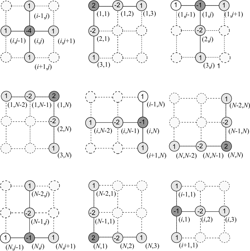
Figure 3: Geometric arrangements and weights to approximate $\mathrm{Lap}_{s}(V)$ at different locations on a grid.

The procedure described in Appendix A can be used to obtain approximations combining more than five electrodes. However, increasing complexity does not result necessarily into more accurate estimates. Approximations for unevenly-spaced electrodes can also be derived, but we will not address this in this paper (cf. Tenke et al., 1998).

Finite difference provides us with a simple measure of accuracy in terms of powers of the discretization parameter $h$. As explained in Appendix A, approximation (20) is said to be accurate to the second-order of $h$, shorthand ${\cal O}(h^{2})$, while for peripheral electrodes the five-point approximations (22) and (23) are accurate to ${\cal O}(h)$. The higher the order, the more accurate is the approximation (Abramowitz and Stegun, 1964). Therefore, in principle, making $h$ small by using high-density electrode arrays should reduce discretization error and improve estimates. Moreover, a small $h$ is useful also to reduce error due to the unrealistic geometry of the plane scalp model, which is more prominent when averaging over sparse electrode sites. In the absence of an appropriate mechanism for regulation, high-density arrays can also help reduce influence of non-local activities from unrelated sources. But exceptions are expected to occur. In fact, all this reasoning was based on the assumption of a point electrode, which ignores boundary effects produced by an actual electrode of finite size. Perhaps for this reason, and due to factors that we are not able to point out, McFarland et al. (1997) reported better estimates using next-nearest-neighbor approximations in comparison to nearest-neighbor approximations. Similar conclusion was drawn by Müller-Gerking et al. (1999) in the context of EEG classification. In fact, next-nearest neighbor approximations have been adopted in CSD analysis since Freeman and Nicholson (1975) as a way to reduce high-frequency noise in the vicinity of an electrode. The trade-off between noise attenuation and loss of spatial resolution in low-density arrays was discussed by Tenke et al. (1993). In fact, lower-density estimates has proven to be quite useful more than once, as described by Kayser and Tenke (2006a) in the context of ERP analysis. Finally, we point out that evidence for electrode bridges in high-density EEG recordings was identified as a problem caused typically by electrolyte spreading between nearby electrodes (Tenke and Kayser, 2001; Greischar et al., 2004; Alschuler et al., 2014).

3.2 Smoothing thin-plate spline Laplacians

As an alternative to finite difference, mesh-free (or grid-free) methods allow for a much more flexible configuration of electrodes and are not restricted to the planar scalp model. In this case, the Laplacian differentiation is performed analytically on a continuous function built from the data. Two ways of obtaining this function are through interpolation or a parametrization procedure known as data smoothing. In the context of interpolation, the problem to be solved can be formulated as follows: given a set of measurements, say a potential distribution $V_{1},\cdots,V_{N}$ recorded from locations $\mathbf{r}_{1},\cdots,\mathbf{r}_{N}$ (the electrode locations), find a real function $f(\mathbf{r})$ such that $f(\mathbf{r}_{i})=V_{i}$ for $i=1,\cdots,N$. For data smoothing, this constraint is replaced with the condition that $f(\mathbf{r}_{i})$ should fit the data closely, but not exactly to reduce variance due to noise. The method of thin-plate splines discussed here is a prime tool for both cases.

Formally, the spline function is the unique solution to the problem of finding a function $f$ that minimizes (Duchon, 1977; Meinguet, 1979; Wahba, 1990; Hastie et al., 2009, p.140)

$$\mathrm{RSS}(f,\lambda)=\frac{1}{N}\sum_{i}\left(V_{i}-f(\mathbf{r}_{i})\right)^{2}+\lambda\thinspace J_{m}\left[f(\mathbf{r})\right],$$ (24)

where it was assumed that $\mathbf{r}_{1}\neq\mathbf{r}_{2}\neq\cdots\neq\mathbf{r}_{N}$ (which is always true for actual electrodes) and $J_{m}\left[f\right]$ is a measure of roughness $f$ in terms of its $m$-th-order partial derivatives (the reader is referred to Wahba, 1990 for details). The parameter $\lambda$ is called the regularization parameter. This parameter trades off between goodness of fit ($\lambda=0$) and smoothness ($\lambda>0$). In other words, if $\lambda=0$ then the interpolation condition $f(\mathbf{r}_{i})=V_{i}$ is satisfied, whereas for $\lambda>0$ the spline function is smooth and violates the interpolation condition. In three-dimensional Euclidean space the solution to this problem has the form (Wahba, 1990; Wood, 2003)

$$f_{\lambda}(\mathbf{r})=\sum_{i=1}^{N}c_{i}\left|\mathbf{r}-\mathbf{r}_{i}\right|^{2m-3}+\sum_{\ell=1}^{M}d_{\ell}\nu_{\ell}(\mathbf{r}),\quad(m\geq 2).$$ (25)

The parameters $m$ and $M$ are integer numbers satisfying $M=\binom{m+2}{3}$ and $M<N$. In addition, $m$ must be greater than 2 for the surface Laplacian differentiation to be well-defined. The functions $\nu_{1},\cdots,\nu_{M}$ are linearly independent polynomials in three variables of degree less than $m$ (Tthe reader is referred to Carvalhaes and Suppes (2011) for the details of how to generate these polynomials).

Using matrix notation we can express the unknowns $c_{i}$’s and $d_{i}$’s as the solution to the linear system (Duchon, 1977; Meinguet, 1979; Wahba, 1990; Green and Silverman, 1994; Eubank, 1999)

$$\left(\begin{array}[]{cc}\mathbf{K}+N\lambda\mathbf{I}&\mathbf{T}\\ \mathbf{T}^{T}&0\end{array}\right)\left(\begin{array}[]{c}\mathbf{c}\\ \mathbf{d}\end{array}\right)=\left(\begin{array}[]{c}\mathbf{v}\\ \mathbf{0}\end{array}\right),$$ (26)

where $\mathbf{c}=(c_{1},\cdots,c_{N})^{T}$, $\mathbf{d}=(d_{1},\cdots,d_{M})^{T}$, $(\mathbf{K})_{ij}=\left|\mathbf{r}_{j}-\mathbf{r}_{i}\right|^{2m-3}$, $(\mathbf{T})_{ij}=\nu_{j}(\mathbf{r}_{i})$, and $\mathbf{v}=(V_{1},\cdots,V_{N})^{T}$ is the given potential distribution. The superscript $T$ indicates transpose operation and $\mathbf{I}$ is the $N\times N$ identity matrix. This system has the formal solution (Wahba, 1990)

$$\mathbf{c}=\mathbf{Q}_{2}\left[\mathbf{Q}_{2}^{T}\left(\mathbf{K}+N\lambda\mathbf{I}\right)\mathbf{Q}_{2}\right]^{-1}\mathbf{Q}_{2}^{T}\mathbf{v},$$ (27a)

$$\mathbf{R}\mathbf{d}=\mathbf{Q}_{1}^{T}\left(\mathbf{v}-\mathbf{K}\mathbf{c}-N\lambda\mathbf{c}\right),$$ (27b)

where $\mathbf{Q}_{1}\in\mathbb{R}^{N\times N}$, $\mathbf{Q}_{2}\in\mathbb{R}^{N\times(N-M)}$, and $\mathbf{R}\in\mathbb{R}^{N\times M}$ derive from the QR-factorization of $\mathbf{T}$ :

$$\mathbf{T}=[\mathbf{Q}_{1}\thinspace|\thinspace\mathbf{Q}_{2}]\begin{pmatrix}\mathbf{R}\\ &\mathbf{0}\end{pmatrix}.$$ (28)

With the above definitions we can express the smoothed potential at the electrode locations as

$$\mathbf{v}_{\lambda}=\mathbf{K}\mathbf{c}+\mathbf{T}\mathbf{d}.$$ (29)

By introducing the matrices $(\tilde{\mathbf{K}})_{ij}=\mathrm{Lap}\left(\left|\mathbf{r}_{j}-\mathbf{r}_{i}\right|^{2m-3}\right)$ and $(\tilde{\mathbf{T}})_{ij}=\mathrm{Lap}\left(\nu_{j}(\mathbf{r}_{i})\right)$, we obtain an analogous expression for the Laplacian estimate, which is

$$\mathrm{Lap}_{S}(\mathbf{v})=\tilde{\mathbf{K}}\mathbf{c}+\tilde{\mathbf{T}}\mathbf{d}.$$ (30)

This approach has a major deficiency, which is that it does not work if the data points $\mathbf{r}_{1},\cdots,\mathbf{r}_{N}$ are located on a spherical or an ellipsoidal surface. To understand this limitation, consider the case $m=3$, for which the matrix $\mathbf{T}$ can be expressed as (Carvalhaes and Suppes, 2011)

$$\mathbf{T}=\left(\begin{array}[]{cccccccccc}1&x_{1}&y_{1}&z_{1}&x_{1}^{2}&x_{1}y_{1}&x_{1}z_{1}&y_{1}^{2}&y_{1}z_{1}&z_{1}^{2}\\ \vdots&\vdots&\vdots&\vdots&\vdots&\vdots&\vdots&\vdots&\vdots&\vdots\\ 1&x_{N}&y_{N}&z_{N}&x_{N}^{2}&x_{N}y_{N}&x_{N}z_{N}&y_{N}^{2}&y_{N}z_{N}&z_{N}^{2}\end{array}\right).$$ (31)

Since on spherical and ellipsoidal surfaces the coordinates $x_{i}$, $y_{i}$, and $z_{i}$ are subject to

$$\frac{x_{i}^{2}}{a^{2}}+\frac{y_{i}^{2}}{b^{2}}+\frac{z_{i}^{2}}{c^{2}}=1,\quad a,b,c>0,$$ (32)

the 1st, 5th, 8th, and 10th columns of $\mathbf{T}$ are linearly dependent. Hence, we can always express one of these columns in terms of the others. This is equivalent to say that $\mathbf{T}$ has 10 columns but only 9 are linearly independent. This makes the linear system (26) singular, so that the unknowns $c_{i}$’s and $d_{i}$’s cannot be uniquely determined.

The singularity of (26) on spheres and ellipsoids affects only the transformation parametrized by $\mathbf{d}$, leaving intact the transformation specified by $\mathbf{c}$. It is therefore natural to try a minimum norm solution to this problem by determining $\mathbf{d}$ using the pseudo-inverse of $\mathbf{R}$, i.e., $\mathbf{d}=\mathbf{R}^{+}\mathbf{Q}_{1}^{\prime}\left(\mathbf{v}-\mathbf{K}\mathbf{c}-N\lambda\mathbf{c}\right)$. This approach was proposed by Carvalhaes and Suppes (2011) (see also Carvalhaes (2013)) and was evaluated in a problem involving the localization of cortical activity on spherical and ellipsoidal scalp models. Simulations using over 30,000 configurations of radial dipoles resulted in a success rate above 94.5% for the correct localization of cortical source at the closest electrode. This rate improved to 99.5% for the task of locating the electrical source at one of the two closest electrode. Prediction error occurred more often for sources generating very small or very large peaks in the amplitude of the potential, but it decreased substantially with increasing the number of electrodes in the simulation. In the same study, but now using empirical data, the surface Laplacian of (25) outperformed finite difference and the method of spherical splines discussed below.

Similar to finite difference, splines and other methods discussed below are usually affected by the density of the electrode array. In general, high-density arrays result in more accurate estimates. However, some preparation issues such as electrolyte bridges are mainly a characteristic of high-density estimates and should be a concern, as it is for finite difference (Tenke and Kayser, 2001). Another concern is that by increasing the number of electrodes the system (26) becomes increasingly sensitive to error (noise) in the input vector $\mathbf{v}$. According to results in Sibson and Stone (1991) it is expected that montages with up to 256 electrodes result in reliable estimates for double-precision calculations, but there is one more issue requiring special attention.

It follows from (27a) that in order to obtain the coefficient vector $\mathbf{c}$ the matrix $[\mathbf{Q}_{2}^{T}\left(\mathbf{K}+N\lambda\mathbf{I}\right)\mathbf{Q}_{2}]$ needs to be inverted. However, it turns out that this inverse operation is accurate only if the condition number of $\left(\mathbf{K}+N\lambda\mathbf{I}\right)$ is relatively small.. In principle, a condition number up to $10^{12}$ should be acceptable for splines (Sibson and Stone, 1991), but this upper bound can easily be exceeded as $\lambda$ decreases toward zero depending on the electrode configuration. In fact, even for a small number of electrodes the condition number of $\left(\mathbf{K}+N\lambda\mathbf{I}\right)$ can be so high that is impossible to invert $[\mathbf{Q}_{2}^{T}\left(\mathbf{K}+N\lambda\mathbf{I}\right)\mathbf{Q}_{2}]$ without regularization. This problem holds also for the algorithm of spherical splines discussed in the next section, and Bortel and Sovka (2007) discussed the same problem in the context of realistic Laplacian techniques. In addition to compensating for conditioning issues, the regularization parameter $\lambda$ determines also the ability of smoothing splines to account for spatial noise in the data. This problem will be addressed in Section 3.6.

3.3 Smoothing spherical splines

For the particular case of data points on spheres, Wahba developed a pseudo-spline method that circumvent the singularity of (26) by replacing the Euclidean distance with the geodesic distance. This method, called spherical splines, was used by Perrin et al. (1989) to developed one of the most popular surface Laplacian methods in the literature. In this case, the smoothing/interpolating function is defined as

$$f_{sph}(\mathbf{r}) = \sum_{i=1}^{N}c_{i}\,g_{m}(\mathbf{r},\mathbf{r}_{i})+d,$$ (33a)

where the parameters $$c_{1},\cdots,c_{N} d$$ and are determined by (27) and

$$g_{m}(\mathbf{r},\mathbf{r}_{i})=\frac{1}{4\pi}\sum_{\ell=1}^{\infty}\frac{2\ell+1}{\ell^{m}(\ell+1)^{m}}P_{\ell}(\mathbf{\hat{r}}\cdot\mathbf{\hat{r}}_{i}).$$ (33b)

The vectors $\mathbf{r}$ and $\mathbf{r}_{i}$’s have length equal to the head radius and carets denote unit vectors, i.e., $\hat{\mathbf{r}}=\mathbf{r}/r$ and $\hat{\mathbf{r}_{i}}=\mathbf{r}_{i}/r$, so that the scalar product $\mathbf{\hat{r}}\cdot\mathbf{\hat{r}}_{i}$ gives the cosine of the angle between $\mathbf{r}$ and $\mathbf{r}_{i}$. The parameter $m$ is an integer larger than 1. The univariable functions $P_{\ell}$’s are Legendre polynomials of degree $\ell$. These polynomials occur in many problems in mathematical physics and their properties are listed in many places Abramowitz and Stegun (e.g. 1964). The infinity summation over Legendre polynomials generates progressively higher spatial frequencies which are weighted by the factor $(2\ell+1)/\ell^{m}(\ell+1)^{m}$. Since this factor decreases monotonically with $\ell$, it acts as a Butterworth filter that downweights high-frequency spatial components to produce a smooth result.

Figure 4: Spherical coordinate system.

To apply the surface Laplacian to (33) we use spherical coordinates. Our convention is that of Figure 4: the polar angle $\theta\in[0,\pi]$ is measured down from the vertex, and the azimuthal angle $\varphi\in[0,2\pi]$ increases counterclockwise from the $x$ axis, which is directed towards the nasion. With this convention,

$$\mathrm{Lap}_{s}(f)=\frac{1}{r^{2}\,\sin\theta}\frac{\partial}{\partial\theta}\left[\sin\theta\frac{\partial f}{\partial\theta}\right]+\frac{1}{r^{2}\sin^{2}\theta}\frac{\partial^{2}f}{\partial\varphi^{2}}.$$ (34)

It can be proved that the Legendre polynomials satisfy (Jackson, 1999, p. 110)

$$\mathrm{Lap}_{s}(P_{\ell}(\mathbf{\hat{r}}\cdot\mathbf{\hat{r}}_{i}))=-\frac{\ell(\ell+1)}{r^{2}}P_{\ell}(\mathbf{\hat{r}}\cdot\mathbf{\hat{r}}_{i}),$$ (35)

thus leading to

$$\mathrm{Lap}_{s}(f(\mathbf{r}))=-\frac{1}{r^{2}}\sum_{i=1}^{N}c_{i}g_{m-1}(\mathbf{r},\mathbf{r}_{i}),\quad m>1,$$ (36)

which is known as the spherical surface Laplacian of $f(\mathbf{r})$.

In comparison to the previous approach, the method of spherical splines has the advantage of providing a simple expression for the surface Laplacian of $f(\mathbf{r})$, although it is restricted to spherical geometry only. Additionally, the geodesic distance ensures that the system (26) is non-singular, so that the coefficient $d$ can be determined without using the pseudo-inverse of $\mathbf{R}$. However, some caution is required. Equation (36) is easy to be implemented, except for the fact that the term $g_{m-1}(\mathbf{r},\mathbf{r}_{i})$ corresponds to an infinite summation. This summation needs to be truncated for evaluation, and truncation error should never be overlooked. The terms that are left out in the truncation of $g_{m-1}(\mathbf{r},\mathbf{r}_{i})$ are Legendre polynomials of higher-degree (large $\ell$) that account for high-frequency spatial features. Too much filtering of such features can overcome the potential for improvement in spatial resolution. In view of that, it is important to keep as many Legendre polynomials as possible in the truncated series. Another point worth considering is the factor $(2\ell+1)/\ell^{m}(\ell+1)^{m}$ that multiplies the Legendre polynomials in equation (33b). This factor falls off as $1/\ell^{2m-1}$. As $\ell$ increases, it approaches zero rapidly, resulting in a quick cancellation of higher-degree polynomials. The value assigned to $m$ must take this effect into account; the larger the value of $m$, the more dramatic is the reduction in high-frequency features. Typically, a value of $m$ between 2 and 6 provides satisfactory results for simulation and data analysis (Babiloni et al., 1995; de Barros et al., 2006; Carvalhaes and Suppes, 2011).

3.4 Other approaches

There are many other possible ways to estimate the surface Laplacian of EEG signals. In this section we briefly review the methods proposed by Yao (2002) and Nunez and collaborators (Law et al., 1993a; Nunez and Srinivasan, 2006). Similar to thin-plate splines, Yao’s approach uses interpolation based on radial functions to estimate the surface Laplacian of the potential. The interpolating function has the general form

$$f_{\mathrm{RBF}}(\mathbf{r})=\sum_{i=1}^{N}c_{i}e^{-\frac{m}{\pi^{2}}S(\mathbf{r},\mathbf{r}_{i})}+b,$$ (37)

where $S(\mathbf{r},\mathbf{r}_{j})$ measures the arc of circle connecting $\mathbf{r}$ and $\mathbf{r}_{i}$ and the parameters $c_{i}$ and $b$ are subject to

$$f_{\mathrm{RBF}}(\mathbf{r}_{i})=V_{i},\quad i=1,\cdots,N,$$ (38)

where $\mathbf{r}_{i}$ is the location of the $i$th electrode and $V_{i}$ is the value of the potential at that location. Because the system (38) contains $N+1$ unknowns but only $N$ equations, it is solved using pseudo-invertion (see the Appendix in Zhai and Yao, 2004).

In contrast to thin-plate splines, the Gaussian function $e^{-\frac{m}{\pi^{2}}S(\mathbf{r},\mathbf{r}_{i})}$ approaches zero asymptotically with growing the distance from the centers $\mathbf{r}_{i}$. The parameter $m$, commonly referred to as the spread parameter, controls the rate of decay of $e^{-\frac{m}{\pi^{2}}S(\mathbf{r},\mathbf{r}_{i})}$. Large values of $m$ produce a sharp decay, resulting in a small range of influence for each node $\mathbf{r}_{i}$. Yao recommended to set $m$ according to the number of electrodes in the montage; for instance, $m=20$ for arrays with 32 sensors, $m=40$ for 64 sensors, and $m=50$ for 128 sensors. But he also remarked that a proper choice of $m$ should take into account the source location. In principle, small values of $m$ would be more suitable to fit deep brain sources, whereas shallow sources would be better described by small $m$-values. In other words, interpolation with Gaussian functions is not automatic. The parameter $m$ needs to be tuned properly for good performance, which can be difficult to achieve for non-equidistant electrodes. Nevertheless, Yao showed consistent results favoring the Gaussian method against spherical splines for simulated and empirical data. More recently Bortel and Sovka (2013) has questioned the regularization technique used by Yao (2002) and the impossibility of obtaining good estimates without a prior knowledge about the source depth.

The method developed by Nunez and collaborators is called the New Orleans Spline-Laplacian (Law et al., 1993a; Nunez and Srinivasan, 2006). This method uses an interpolating function that resembles two-dimensional splines but with knots in $\mathbb{R}^{3}$ instead of $\mathbb{R}^{2}$, i.e.,

$$f_{\mathrm{NOSL}}(\mathbf{r}) = \sum_{i=1}^{N}c_{i}\left|\mathbf{r}-\mathbf{r}_{i}\right|{}^{4}\log(\left|\mathbf{r}-\mathbf{r}_{i}\right|{}^{2}+\omega^{2})+d_{1}+d_{2}x+d_{3}y$$ (39)

$$+ d_{4}z+d_{5}x^{2}+d_{6}xy+d_{7}xz+d_{8}y^{2}+d_{9}yz+d_{10}z^{2},$$

where the parameters $c_{i}$’s and $d_{i}$’s are determined in the fashion of equation (26). This method was implemented for spherical and ellipsoidal scalp models and its performance was studied using simulations and real data (Law et al., 1993a). A remark about the function $f_{\mathrm{NOSL}}(\mathbf{r})$ is that it has no optimality property, except that for $\omega$ and $z$ equal to zero it corresponds to the unique minimizer of (24) in $\mathbb{R}^{2}$ (Duchon, 1977; Meinguet, 1979). But $f_{\mathrm{NOSL}}(\mathbf{r})$ does not minimize (24) in $\mathbb{R}^{3}$, as the minimizer of (24) in $\mathbb{R}^{3}$ is unique and correspond to the spline function (25). Or, putting it in other words, $f_{\mathrm{NOSL}}(\mathbf{r})$ is not actually a spline function. Despite that, Nunez and colleagues reported many studies showing a good performance of their method (Law et al., 1993b; Nunez and Westdorp, 1994; Nunez et al., 2001; Nunez and Srinivasan, 2006) and emphasized its agreement with cortical imaging algorithms in terms of correlation (Nunez et al., 1993, 1994).

3.5 The surface Laplacian matrix

The computational cost of estimating the surface Laplacian is usually not prohibitive, but in the majority of circumstances it is high enough to justify the use of an additional technique to improve performance. The surface Laplacian matrix, denoted by $\mathbf{L}$, is an excellent tool for this purpose, and because of the linearity of the Laplacian differentiation, it can be created for any of the Laplacian methods discussed in this paper. For interpretation purposes the surface Laplacian matrix can be viewed as a discrete representation of the differential operator $\mathrm{Lap}_{S}$ at the electrode sites. We will illustrate the method for finite difference and splines. Once the matrix $\mathbf{L}$ is obtained the Laplacian estimate is carried out through the linear transformation

$$\mathrm{Lap}_{S}(\mathbf{v})=\mathbf{L}\mathbf{v}.$$ (40)

An important aspect of $\mathbf{L}$ is that its construction does not use brain data, as otherwise it could not represent the mathematical operator $\mathrm{Lap}_{S}$. This way we need to create $\mathbf{L}$ only once for each method and electrode configuration. But notice that $\mathbf{L}$ depends on the parameters $m$ and $\lambda$ for splines.

We will first illustrate the construction of $\mathbf{L}$ for finite difference approximations. In this case, $\mathbf{L}$ is constructed row by row using the scheme of Figure 3. Electrodes that do not contribute to an approximation are assigned a zero weight in that computation. This way, each row of $\mathbf{L}$ has as many elements as the number of channels in the montage, but only five elements are nonzero in each row. This implies that $\mathbf{L}$ is a sparse matrix, with its sparsity increasing with the number of channels. Because the weights of each approximation sum to zero, the columns of $\mathbf{L}$ also sum to zero, which reflects the fact that the Laplacian transformation is reference-free.

As a simple illustration, consider the electrode arrangement of Figure 5, with 9 electrodes evenly distributed in a square grid of spacing $h$.

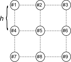
Figure 5: A montage with 9 electrodes in a square grid of spacing $h$. The numbers 1 to 9 identify the electrodes and should not be confused with the weights for a finite difference approximation.

The Laplacian matrix of this arrangement has dimension $9\times 9$ and is given by

$$\mathbf{L}=\frac{1}{h^{2}}\begin{pmatrix}\begin{array}[]{rrrrrrrrr}2&-2&1&-2&0&0&1&0&0\\ 1&-1&1&0&-2&0&0&1&0\\ 1&-2&2&0&0&-2&0&0&1\\ 1&0&0&-1&-2&1&1&0&0\\ 0&1&0&1&-4&1&0&1&0\\ 0&0&1&1&-2&-1&0&0&1\\ 1&0&0&-2&0&0&2&-2&1\\ 0&1&0&0&-2&0&1&-1&1\\ 0&0&1&0&0&-2&1&-2&2\end{array}\end{pmatrix}.$$ (41)

A quick inspection on the diagonal elements of $\mathbf{L}$ reveals that none of them is equal to zero, but they sum to zero. This means that $\mathbf{L}$ does not possess inverse. The inability to invert $\mathbf{L}$ is not exclusive of finite differences, but rather a general property that reflects the ambiguity on the choice of reference. Stated in other words, the Laplacian transformation (40) cannot be uniquely undone due to the fact that the potential is not uniquely defined.

Mesh-free methods generate $\mathbf{L}$ matrices that are non-sparse, i.e., most of their entries are nonzero. In the context of smoothing splines, Carvalhaes and Suppes (2011) showed that

$$\mathbf{L}_{\lambda}=\tilde{\mathbf{K}}\,\mathbf{C}_{\lambda}+\tilde{\mathbf{T}}\,\mathbf{D}_{\lambda},$$ (42)

where the subscript $\lambda$ emphasizes dependency on the regularization parameter, and

$$(\tilde{\mathbf{K}})_{ij}=\mathrm{Lap}_{s}\left(\left|\mathbf{r}_{i}-\mathbf{r}_{j}\right|^{2m-3}\right),$$ (43a)

$$(\tilde{\mathbf{T}})_{ij}=\mathrm{Lap}_{s}\left(\nu_{i}(\mathbf{r}_{j})\right),$$ (43b)

$$\mathbf{C}_{\lambda}=\mathbf{Q}_{2}\left[\mathbf{Q}_{2}^{T}\left(\mathbf{K}+N\lambda\mathbf{I}\right)\mathbf{Q}_{2}\right]^{-1}\mathbf{Q}_{2}^{T},$$ (43c)

$$\mathbf{D}_{\lambda}=\mathbf{R}^{+}\mathbf{Q}_{1}^{T}\left(\mathbf{1}-\mathbf{K}\mathbf{C}_{\lambda}-N\lambda\mathbf{C}_{\lambda}\right).$$ (43d)

The matrix $\mathbf{L}_{\lambda}$ also has no inverse, thus not allowing unambiguous inverse operation. This is due to the fact that $\mathbf{C}_{\lambda}$ and $\tilde{\mathbf{T}}$ are rank-deficient. In other words, since $\mathbf{Q}_{2}$ has only $N-1$ columns, only $N-1$ degrees of freedom are available from $\mathbf{C}_{\lambda}$. In turn, because the Laplacian operation $\mathrm{Lap}_{s}(\nu_{i}(\mathbf{r}_{j}))$ vanishes at any polynomial $\nu_{i}$ of degree less than 2, the first four columns of $\tilde{\mathbf{T}}$ are null.

For spherical splines, $(\mathbf{\tilde{\mathbf{K}}})_{ij}=-g_{m}(\mathbf{r}_{j},\mathbf{r}_{i})/r^{2}$, $\mathbf{T}$ is a $N$-vector of ones, and $\tilde{\mathbf{T}}$ is null, so that

$$\mathbf{L}_{\lambda}=\tilde{\mathbf{K}}\,\mathbf{C}_{\lambda},$$ (44)

which has rank $N-1$ and does not possess inverse. Since $\mathbf{T}$ is a vector of ones, its QR-factorization gives $\mathbf{R}=-\sqrt{N}$, i.e., $\mathbf{R}$ is a scalar instead of a matrix, and $\mathbf{Q}_{1}=-\mathbf{T}/\sqrt{N}$. Consequently, $\mathbf{D}_{\lambda}=\mathbf{T}^{T}\left(\mathbf{1}-\mathbf{K}\mathbf{C}_{\lambda}-N\lambda\mathbf{C}_{\lambda}\right)/N$, which is also a $N$-vector instead of a matrix.

As anticipated, the construction of $\mathbf{L}$ and $\mathbf{L}_{\lambda}$ is carried out without using brain data. Because the matrix $\mathbf{C}_{\lambda}$ depends on the inverse of the matrix $[\mathbf{Q}_{2}^{T}\left(\mathbf{K}+N\lambda\mathbf{I}\right)\mathbf{Q}_{2}]$ it is subject to the numerical issues discussed in Section 3.2, so that it is a good measure to set $\lambda$ different from zero and keep $m$ as small as possible for accurate results.

The computational cost of estimating the Laplacian can be expressed in terms of the number of floating-point operations (flops) required by (40). The computational cost of finite difference is generally much smaller than the cost of splines. Assume that $\mathbf{v}$ in (40) is a matrix containing $N$ rows, each one corresponding to an electrodes, and $T$ columns, which one representing a time frame. The cost of computing (40) using finite difference is $5NT$ flops, which is equivalent to the number of nonzero elements in $\mathbf{L}$ times the number of time frames. Putting in numbers, handling 5 minutes of recordings at 1 kHz sampling rate costs $5\times 32\times 18000=2,880,000$ flops for $N=32$ electrodes. This cost is much higher in the spline framework. Because $\mathbf{L}_{\lambda}$ is not sparse, the cost of computing (40) is $N^{2}T$ flops, or 18,432,000 flops for the above example. However, without using the Laplacian matrix the system (26) needs to be solved once for each frame at the cost of $(2/3)\leavevmode\nobreak\ N^{3}$ flops per frame, which brings the figure to over 6 billion flops.

3.6 The regularization of smoothing splines

The use of smoothing splines to estimate the surface Laplacian requires the estimate of the regularization parameter $\lambda$, which, as said above, has the beneficial effect of eliminating spatial noise through variance reduction. A key factor to guide towards a good choice of $\lambda$ is the mean square error function

$$R(\lambda)=\frac{1}{N}\sum_{i=1}^{N}\left(V_{i}-f_{\lambda}(\mathbf{r}_{i})\right)^{2}.$$ (45)

Intuitively, this function measures infidelity of $f_{\lambda}(\mathbf{r})$ to the input data ($V_{1},\cdots,V_{N}$) due to smoothing. The goal of regularization is to weight this function appropriately to achieve a good balance between fidelity and variance reduction. The popular method of generalized cross-validation (GCV) proposed by Craven and Wahba (1979) addresses this problem in the following way. The GCV estimate of $\lambda$ is the value for which the function

$$\mathrm{GCV}(\lambda)=\frac{1}{N}\frac{\sum_{i=1}^{N}\left(V_{i}-f_{\lambda}(\mathbf{r}_{i})\right)^{2}}{\left(1-\mathrm{trace}(\mathbf{S}_{\lambda})/N\right)^{2}},$$ (46)

reaches its minimum value. Here, $\mathbf{S}_{\lambda}$ is a $N\times N$ matrix satisfying

$$\begin{pmatrix}f_{\lambda}(\mathbf{r}_{1})\\ \vdots\\ f_{\lambda}(\mathbf{r}_{N})\end{pmatrix}=\mathbf{S}_{\lambda}\begin{pmatrix}V_{1}\\ \vdots\\ V_{N}\end{pmatrix}.$$ (47)

In other words, the GCV criterion corrects the squared residuals $\left(V_{i}-f_{\lambda}(\mathbf{r}_{i})\right)^{2}$ about the estimate by dividing them by the factor $(1-\mathrm{trace}(\mathbf{S}_{\lambda})/N)^{2}$. The value $\lambda=0$ is excluded from predictions because for $\lambda=0$ (47) is turned into a regression problem for which $\mathrm{trace}(\mathbf{S}_{\lambda})=N$, which vanishes the denominator of (46).

The matrix $\mathbf{S}_{\lambda}$ is called the smoother matrix. It follows from our previous development that

$$\mathbf{S}_{\lambda}=\mathbf{K}\,\mathbf{C}_{\lambda}+\mathbf{T}\,\mathbf{D}_{\lambda}.$$ (48)

Since this expression involves no differentiation, it is relatively simple to compute $\mathbf{S}_{\lambda}$ on any scalp model. Another observation is that the columns of $\mathbf{S}_{\lambda}$ sum to 1 (whereas the columns of $\mathbf{L}_{\lambda}$ sum to 0), implying that the transformation (47) preserves the reference potential.

In practice, the search for $\lambda$ is constrained to a finite interval which typically spans several decades on a log scale (Babiloni et al., 1995). In order to facilitate interpretation and comparisons across studies, instead of thinking in terms of $\lambda$ it is convenient to think in terms of a parameter $\mathrm{DF}_{\lambda}$ that has more practical meaning. The parameter $\mathrm{DF}_{\lambda}$ is called the effective degree of freedom of $f_{\lambda}(\mathbf{r})$ and is defined by (Hastie et al., 2009; James et al., 2013)

$$\mathrm{DF}_{\lambda}=\mathrm{trace}(\mathbf{S}_{\lambda}),$$ (49)

where the trace operation sums over the diagonal elements of $\mathbf{S}_{\lambda}$. This operation assigns a real value to $\mathrm{DF}_{\lambda}$ between 1 and $N$. The lower bound of $\mathrm{DF}_{\lambda}$ accounts for the linear portion of $f_{\lambda}(\mathbf{r})$, whereas the upper bound corresponds to $\lambda=0$, for which $\mathbf{S}_{\lambda}$ is the projection matrix from regression over $(V_{1},\cdots,V_{N})^{T}$ which has trace equal to $N$.

In order to think in terms of $\mathrm{DF}_{\lambda}$ instead of $\lambda$ we need to invert the relation (49). This inversion is possible but it can only be done numerically. Figure 6 depicts the situation for a montage with 32 sensors. Although $\mathrm{DF}_{\lambda}$ is shown as if it were the independent variable, its values were actually determined from (49) by fixing $\lambda$. The Matlab code of Appendix B was used to compute $\mathbf{S}_{\lambda}$. This code implements the spherical splines algorithm of Section 3.3 with a default error tolerance of less than $1\times 10^{-10}$ in the computation of the infinity series (33b). The electrode locations were normalized to a sphere of radius 10 cm. Figure 6 shows that $\mathrm{DF}_{\lambda}$ decreases monotonically with $\lambda$. Thanks to monotonicity we can interpolate the pairs $(\mathrm{DF}_{\lambda},\lambda)$ to obtain a continuous curve from which we can estimate $\lambda$ given $\mathrm{DF}_{\lambda}$.

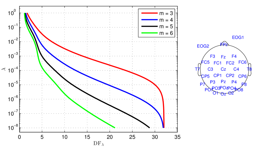
Figure 6: The monotonically decreasing relationship between $\mathrm{DF}_{\lambda}$ and $\lambda$ for a montage with 32 electrodes (right). Each solid line indicates a distribution with 100 values of $\lambda$ in the range of $10^{-8}$ to 1 on a log scale. The different colors indicate the value of the parameter $m$ used in the calculation.

To fix ideas lets consider an example with real brain data. The data that will be used here were extracted from a sample dataset distributed with the EEGLab Matlab Toolbox, version 13.2.2b (Delorme and Makeig, 2004). Our goal is simply to illustrate the regularization procedure in a way that can be easily reproduced by the reader. The ready availability of this dataset is very suitable for this purpose. The data contain 30,504 frames recorded from 32 channels at a sampling rate of 128 Hz. We arbitrarily chose the frame of number 200 for exploration. Our computations were carried out using spherical splines with $m=4$ (see Appendix B). The electrode configuration was the same as in Figure 6. The following steps were followed:

1. Create a grid of values of $\mathrm{DF}_{\lambda}$ between 2 and 31 in increments of 1.

2. Calculate the values of $\lambda$ from $\mathrm{DF}_{\lambda}$ by means of interpolation.

3. Compute the GCV score of each pair $\mathrm{DF}_{\lambda}$ and $\lambda$ from (46).

4. Interpolate the pairs $(\mathrm{DF}_{\lambda},\mbox{GCV})$ to obtain a continuous error curve.

5. Find the optimal value $\hat{\mathrm{DF}}_{\lambda}$ that minimizes the error curve.

Step 1 is the only step of this sequence that depends on the electrode configuration, with the upper bound of $\mathrm{DF}_{\lambda}$ depending on the number of electrodes. The Matlab function interp1 was used to perform step 2, whereas steps 4 and 5 were carried out using csapis, fnval, and fminbnd.

The error curve is depicted in Figure 7. The optimal value of $\mathrm{DF}_{\lambda}$ was $\hat{\mathrm{DF}}_{\lambda}=8.82$, corresponding to a reduction by about 72% in degrees of freedom. Figure 8 shows a plot of the smooth potential for this value of $\hat{\mathrm{DF}}_{\lambda}$. Note an important change in topography due to regularization. While the raw potential exhibits two prominent peaks at electrodes 7 (FC5) and 9 (FC2), which suggests the presence of a pair of dipoles of same polarity interposed by FC1, the regularized potential points out the existence of a single dipole in the region enclosed by Fz, FC1, FC2, and Cz (electrodes 4, 8, 9, and 14).

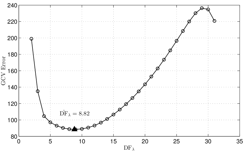
Figure 7: An illustration of the GCV regularization. The error curve reached its minimum value at $\hat{\mathrm{DF}}_{\lambda}=8.82$.

Figure 8: Spline fit (filled circles) of the sample potential (empty circles) using $\mathrm{DF}_{\lambda}=8.82$. The solid line is only a guide to the eye.

In this example the potential distribution was re-referenced to the average before regularization, but because the smoother matrix preserves the reference, both before and after regularization it had zero mean, as can be inferred from Figure 8. We also remark that the theory underlying GCV is asymptotic, so that a few outliers should be expected for $N$ small. For this reason the error function should be minimized by constraining the solution to the extremes of the interval in step 1.

We will now focus on a problem of more practical interest, which is the simultaneous regularization of multiple frames. In principle, the above procedure applies immediately if we construct the spline function in $\mathbb{R}^{4}$ instead of $\mathbb{R}^{3}$ by taking time as a fourth coordinate. However, it is not difficult to see that this cannot work in practice, because of dimensionality. For instance, a data sample with 32 channels as above and just 100 frames sets the dimension of the system (26) to 3,200$\times$3,200, which is far beyond the limit of validity of splines. Due to this problem EEG systems containing more than 100 channels are unfeasible to be dealt with splines in $\mathbb{R}^{4}$ even for a small number of frames. For $N$ small we could think of slicing the data into small non-overlapping sets for regularization, but it is questionable if this can improve to much on frame-by-frame regularization in $\mathbb{R}^{3}$. So, let us continue to work with splines in $\mathbb{R}^{3}$.

Although the GCV algorithm is relatively simple and requires modest computational resources and time, its sequential application over multiple frames can be costly. In addition, it is very unlikely that outcomes from independent regularizations would agree upon a global estimate of $\hat{\mathrm{DF}}_{\lambda}$, and dealing with a distribution of $\hat{\mathrm{DF}}_{\lambda}$ lacks flexibility and simplicity sought so far. Of course, we could average across GCV estimates to determine a global $\hat{\mathrm{DF}}_{\lambda}$, but there is no reason to believe that this distribution is stationary and has a central tendency. Viewed from a statistical perspective, it would be more interesting to seek an optimality criterion that applies at once to the entire dataset. In light of this commitment we suggest a modification to the GCV algorithm, expressed as follows

$$\overline{\mathrm{GCV}}(\lambda)=\frac{\sum_{i=1}^{N}\sum_{t=1}^{T}\left(V_{i,t}-f_{\lambda,t}(\mathbf{r}_{i})\right)^{2}}{NT\left(1-\mathrm{DF}_{\lambda}/N\right)^{2}},$$ (50)

where $T$ is the total number of frames and $V_{i,t}$ and $f_{\lambda,t}$ are the potential and the estimated spline function on frame $t$. That is, each value of $\mathrm{DF}_{\lambda}$ is now scored according to its global effect across all frames rather than on a single frame. The weight $1/\left(1-\mathrm{DF}_{\lambda}/N\right)^{2}$ assigned to each choice of $\mathrm{DF}_{\lambda}$ remains the same, but now closeness of fit as measured by mean square error is influenced by all residuals at once, which justifies the term $1/NT$ to normalize the square error. Another way of putting it is that the $\overline{\mathrm{GCV}}$ estimate of $\hat{\mathrm{DF}}_{\lambda}$ is the value of $\mathrm{DF}_{\lambda}$ that minimizes the mean GCV error function $\overline{\mathrm{GCV}}(\lambda)=\sum_{t=1}^{T}\mathrm{GCV}_{t}(\lambda)/T$.

We applied this criterion to regularize the above dataset for all frames. Except that equation (50) instead of (46) was used to compute error scores, the same 5-step procedure of the previous example was followed. Figure 9 depicts the error curve. The estimated value of $\hat{\mathrm{DF}}_{\lambda}$ is $14.05$, which differs significantly from the previous example.

Figure 9: Global regularization using the $\overline{\mathrm{GCV}}$ criterion.

4 Concluding Remarks

The literature on the surface Laplacian technique is quite large and this paper could only partially review or expand a few topics of general importance. It was our primary goal to give a more intuitive view of the technique by providing physical insights that are often missing in the literature. In addition, we discussed several numerical methods to estimate the Laplacian, each one has its own set of strengths and limitations which we tried to clarify. Because of popularity, special attention was given to the methods of finite difference and splines. Finite difference is arguably one of the simplest approach for Laplacian estimates and its computational cost is highly encouraging, mainly for EEG experiments involving a large number of electrodes. The major disadvantage, however, is that estimates are prone to discretization errors and regularized estimates to eliminate spatial noise are not provided. Splines are still the main alternative to finite difference in EEG literature. The need for evenly-spaced electrodes and other problems related to discretization are totally eliminated, the scalp geometry becomes more realistic, and spatial noise that otherwise is amplified by Laplacian differentiation are reduced through regularization. The cost of such improvement is not negligible and is reflected in a increase in mathematical complexity and a higher computational cost compared to finite difference. Moreover, it worth remarking that splines are also sensitive to error in electrode locations (e.g. Bortel and Sovka, 2008) and the belief that accurate estimates at peripheral electrodes are made possible is not entirely correct. In fact, note that the construction of $f_{\lambda}(\mathbf{r})$ involves $N+M$ unknowns, which are the coefficients $c_{i}$’s and $d_{i}$’s in (25) and (33a), but only $N$ observations are available for each frame, which are the measured potentials $V_{1},\cdots,V_{N}$. To avoid underdetermination, the system (26) contains an ad hoc condition $\mathbf{T}^{T}\mathbf{c}=0$ that adds $M$ more constraint to $f_{\lambda}(\mathbf{r})$, which has the geometric effect of canceling terms from $f_{\lambda}(\mathbf{r})$ that grow faster than a polynomial of degree $m$ as one moves away from the electrodes. Estimates at central and peripheral electrodes are affected differently by this condition, with estimates at peripheral electrodes being less accurate. Unfortunately, it was outside the scope of our work to discuss methods to make the scalp model more realistic and reduce error in electrode locations, as they require additional tools such as MRI that are often not readily available to most researchers. The interested reader is referred to the relevant references for this matter (Le and Gevins, 1993; Gevins et al., 1994; Le et al., 1994; Babiloni et al., 1996; Bortel and Sovka, 2013).

Our discussion on computational methods emphasized our recommendation to set the spline parameter $m$ as equal to 3 or 4 to avoid numerical issues. We can use the result in Figure 6 to get further insight into this problem. This example clearly shows a compromise between the value of $m$, the effective number of degrees of freedom of the spline fit, and the lower bound of the $\lambda$ parameter. Namely, although small and large values of $m$ appear equally suitable to assess low degrees of freedom, say $\mathrm{DF}_{\lambda}<10$, the fact that $\lambda$ is bounded from below at $10^{-8}$ prevents us from exploiting the region of $\mathrm{DF}_{\lambda}>20$ properly without setting $m=3$ or 4. One may think of a way to circumvent this limitation by decreasing the lower bound of $\lambda$ toward zero, but as explained in Section 3.2 this has the problem of impoverishing the numerical conditioning, thus reinforcing our recommendation stated above.

Yet, despite the broad literature on the subject, some basic problems on Laplacian estimates are still unsolved. Our effort to contribute to such questions is reflected in a new set of approximations for Laplacian estimates on the grid and a workable solution to the problem of global regularization. One difficult problem that could not be addressed is related to the finite size of measuring electrodes. All computational methods discussed here were built upon the idea of a point-like electrode, but an actual electrode has a finite size and for this reason EEG potentials should be interpreted as spatial averages instead of point values. From a computational perspective, a similar problem occurs in the approximation of a histogram by a continuous function in statistics (the density function), which has led to the concept of histopolation (Boneva et al., 1971; Wahba, 1976). The solution consisted basically of replacing the point interpolation condition $y_{i}=f(x_{i})$ by the area matching condition $y_{i}=\int_{ih}^{(i+1)h}f(x)\thinspace dx$, where $h$ is the “bin size”. An extension to two-dimensional space was straightforward and has led to the variational problem of minimizing

$$\mbox{RSS}(f,\lambda)=\frac{1}{N}\sum_{i}\left[V_{i}-\iint_{\Omega_{i}}f(\mathbf{r}_{i})\thinspace dA\right]^{2}+\lambda\thinspace J_{m}\left[f\right].$$ (51)

Wahba (1981) studied this problem in Euclidean space and used the GCV statistics as explained here to estimate the optimal parameter $\lambda$. A similar approach could be sought on the sphere to account for finite-sized electrodes on a spherical scalp model, taking the double integral over the finite area of each electrode. This problem is arguably not trivial and almost certainly will require a numerical solution. Yet this a simplified model that does not address the much more complicate problem of boundary effects due to the highly conductive electrode over the region $\Omega_{i}$.

Considerable attention was devoted to the method of estimating the Laplacian derivation by means of a linear transformation, for which some figures were given estimating computational costs and encouraging the use of this procedure, mainly in the context of splines. Similar attention was paid to the problem of regularization across multiple frames to improve estimates, for which we suggested a possible solution based on generalized cross-validation. It is worth remarking that spatial regularization is not useful to eliminate noise coming from the reference electrode. In fact, because spline fits preserves the reference signal, the residuals $\varepsilon_{i}=V_{i}-f_{\lambda}(\mathbf{r}_{i})$ are reference-free, and so are the error functions GCV and $\overline{\mathrm{GCV}}$, making evident that any noise due to the reference is fully preserved by regularization. This problem, however, should not cause any concern since it simply does not exist in the context of surface Laplacian analysis.

Finally, we want to mention our effort in recent papers to develop a vector form of EEG that combines the surface Laplacian and the tangential components of the electric field projected on the scalp surface (Wang et al., 2012; Carvalhaes et al., 2014). This combination was grounded on the observation that the surface Laplacian derivation is closely related to the spatial component of the electric field oriented normally to the scalp surface, thus not containing substantial information about features encoded in tangential direction. Not surprisingly, this combination of physically distinct but somewhat supplementary quantities resulted in significant improvement for a variety of classification tasks as described in Carvalhaes et al. (2014).

Appendix A The mathematics Behind Finite Difference

A systematic way to obtain finite difference approximations for the derivatives of a function is based on the Taylor series expansion. To expand in terms of Taylor series, we formulate the problem in terms of a continuous function $V$ and then, for compatibility with our notation in Section 3.1, rewrite the final approximation using discrete variables. In its simplest case, the Taylor series of a univariate function $V(x)$ around a point $x=a$ is defined by the infinite summation

$$V(a+h)=V(a)+V^{\prime}(a)h+\frac{1}{2!}V^{\prime\prime}(a)h^{2}+\frac{1}{3!}V^{\prime\prime\prime}(a)h^{3}+\cdots,$$ (52)

where $h$ is called the increment, $n!=n(n-1)(n-2)\cdots 1$ is the factorial of $n$, and $V^{(n)}\left(a\right)$ denotes the $n$-th derivative of $V(x)$ at $x=a$. That is, the Taylor series of $V(x)$ is a power series of $h$ with coefficients given by the derivatives of $V(x)$ at $x=a$. To obtain an approximation for the second derivative (or any other derivative) of $V(x)$ at $x=a$ we proceed as follows. Replace $h$ with $-h$ in (52) and obtain an analogous expression for $V(a-h)$, i.e.,

$$V(a-h)=V(a)-V^{\prime}(a)h+\frac{1}{2!}V^{\prime\prime}(a)h^{2}-\frac{1}{3!}V^{\prime\prime\prime}(a)h^{3}+\cdots$$

Adding these two expressions,

$$V(a+h)+V(a-h)=2V(a)+V^{\prime\prime}(a)h^{2}+\frac{1}{12}V^{iv}(a)h^{4}+\cdots,$$

whence

$$V^{\prime\prime}(a)=\frac{V(a+h)+V(a-h)-2V(a)}{h^{2}}-\frac{1}{12}V^{iv}(a)h^{2}-\cdots,$$ (53)

Assuming that $h$ is sufficiently small we can ignore all terms containing powers of $h$ and arrive at

$$V^{\prime\prime}(a)\approx\frac{V(a+h)+V(a-h)-2V(a)}{h^{2}}.$$

Replacing $a=(i-1)\,h$, $i=2,\cdots,N-1$, and using the notation $V_{i}=V(a)$ and $V_{i\pm 1}=V(a\pm h)$ yields

$$V^{\prime\prime}(a)\approx\frac{V_{i+1}+V_{i-1}-2V_{i}}{h^{2}}.$$ (54)

This expression was obtained by truncating the infinite series (53) after the first term. This way, starting from $h^{2}$ all powers of $h$ were eliminated assuming that $h$ was sufficiently small. The result was a second-order approximation, which in the “big-Oh” notation is referred to as ${\cal O}(h^{2})$.

Approximation (54) excludes the case of a peripheral node, for which either $V_{i+1}$ or $V_{i-1}$ does not exist. In this case, we have to build the approximation using only nodes to the right or left of $a$, but not both. For instance, let $i=1$ and use the expansions

$$V(a+h)=V(a)+V^{\prime}(a)h+\frac{1}{2}V^{\prime\prime}(a)h^{2}+\frac{1}{6}V^{\prime\prime\prime}(a)h^{3}+\cdots,$$

$$V(a+2h)=V(a)+2V^{\prime}(a)h+2V^{\prime\prime}(a)h^{2}+\frac{4}{3}V^{\prime\prime\prime}(a)h^{3}+\cdots,$$

from which

$$V(a+2h)-2V(a+h)=-V(a)+V^{\prime\prime}(a)h^{2}+V^{\prime\prime\prime}(a)h^{3}+\cdots$$

and

$$V^{\prime\prime}(a)=\frac{V(a+2h)-2V(a+h)+V(a)}{h^{2}}-V^{\prime\prime\prime}(a)h-\cdots$$

In terms of the grid variables,

$$V^{\prime\prime}(a)\approx\frac{V_{3}-2V_{2}+V_{1}}{h^{2}},$$ (55)

which is a first order approximation. Note that this expression corresponds to the formula obtained by Freeman and Nicholson (1975) for one-dimensional estimate of intracranial CSD.

A.1 Bivariate functions and approximations for $\mathrm{Lap}(V(a,b))$

The extension of (52) to bivariate functions replaces ordinary derivatives with partial derivatives. Namely,

$$V(a+h_{1},b+h_{2})=V(a,b)+\left[\frac{\partial V(a,b)}{\partial x}h_{1}+\frac{\partial V(a,b)}{\partial y}h_{2}\right]+\frac{1}{2}\left[\frac{\partial^{2}V(a,b)}{\partial x^{2}}h_{1}^{2}+2\frac{\partial^{2}V(a,b)}{\partial x\partial y}h_{1}h_{2}\right.\\ \left.+\frac{\partial^{2}V(a,b)}{\partial y^{2}}h_{2}^{2}\right]+\frac{1}{6}\left[\frac{\partial^{3}V(a,b)}{\partial x^{3}}h_{1}^{3}+3\frac{\partial^{3}V(a,b)}{\partial^{2}x\partial y}h_{1}^{2}h_{2}+3\frac{\partial^{3}V(a,b)}{\partial x\partial^{2}y}h_{1}h_{2}^{2}+\frac{\partial^{3}V(a,b)}{\partial y^{3}}h_{2}^{2}\right]+\cdots\,\,.$$ (56)

Similar to the one-dimensional case, with appropriate choices for $h_{1}$ and $h_{2}$ one can use this expansion to approximate the partial derivatives of $V(x,y)$ at any point in a rectangular grid. An approximation for the Laplacian of $V(x,y)$ at a central node of a square grid ($h_{1}=h_{2}=h$) is obtained as follows. First, use (56) to expand $V(a\pm h,b)$ and $V(a,b\pm h)$:

$$V(a\pm h,b) =V(a,b)\pm\frac{\partial V(a,b)}{\partial x}h+\frac{1}{2}\frac{\partial^{2}V(a,b)}{\partial x^{2}}h^{2}\pm\frac{1}{6}\frac{\partial^{3}V(a,b)}{\partial x^{3}}h^{3}+\frac{1}{24}\frac{\partial^{4}V(a,b)}{\partial x^{4}}h^{4}\pm\cdots,$$

$$V(a,b\pm h) =V(a,b)\pm\frac{\partial V(a,b)}{\partial y}h+\frac{1}{2}\frac{\partial^{2}V(a,b)}{\partial y^{2}}h^{2}\pm\frac{1}{6}\frac{\partial^{3}V(a,b)}{\partial y^{3}}h^{3}+\frac{1}{24}\frac{\partial^{4}V(a,b)}{\partial y^{4}}h^{4}+\cdots.$$

Second, add these four expressions to obtain

$$V(a+h,b)+V(a-h,b)+V(a,b+h)+V(a,b-h)=4V(a,b)+\underset{\mathrm{=Lap}(V(a,b))}{\underbrace{\left[\frac{\partial^{2}V(a,b)}{\partial x^{2}}+\frac{\partial^{2}V(a,b)}{\partial y^{2}}\right]}}h^{2}\\ +\frac{1}{12}\left[\frac{\partial^{4}V(a,b)}{\partial x^{4}}+\frac{\partial^{4}V(a,b)}{\partial y^{4}}\right]h^{4}+\cdots,$$

whence

$$\mathrm{Lap}(V(a,b))=\frac{V(a+h,b)+V(a-h,b)+V(a,b+h)+V(a,b-h)-4V(a,b)}{h^{2}}+{\cal O}(h^{2}).$$

Therefore, $\mathrm{Lap}(V(a,b))$ is approximated to the second-order of $h$ by

$$\mathrm{Lap}(V(a,b))\approx\frac{V(a+h,b)+V(a-h,b)+V(a,b+h)+V(a,b-h)-4V(a,b)}{h^{2}}.$$

This expression is equivalent to Hjorth’s Laplacian estimate, which is shown in (20) with $V_{(i,j)}=V(a,b)$, $V_{(i\pm 1,j)}=V(a,b\mp h)$, and $V_{(i,j\pm 1)}=V(a\pm h,b)$.

A.2 Approximations for peripheral electrodes

Suppose that we want to approximate $\mathrm{Lap}(V)$ at a point $(a,b)$ which is outside the domain of $V$. Let us start with a node in the left border of the grid, but not in a corner. Our mapping from the continuous variables $x$ and $y$ into the discrete variables $i$ and $j$ follows $x=(j-1)\thinspace h$ and $y=(N-i+1)\thinspace h$. See also the scheme in Figure 2. For a node on the left border $x=0$, which corresponds to the first column of the grid ($j=1$). The Taylor series of interest are

$$V(h,b) =V(0,b)+\frac{\partial V(0,b)}{\partial x}h+\frac{1}{2}\frac{\partial^{2}V(0,b)}{\partial x^{2}}h^{2}+\frac{1}{6}\frac{\partial^{3}V(0,b)}{\partial x^{3}}h^{3}+\frac{1}{24}\frac{\partial^{4}V(0,b)}{\partial x^{4}}h^{4}+\cdots,$$

$$V(2h,b) =V(0,b)+2\frac{\partial V(0,b)}{\partial x}h+2\frac{\partial^{2}V(0,b)}{\partial x^{2}}h^{2}+\frac{4}{3}\frac{\partial^{3}V(0,b)}{\partial x^{3}}h^{3}+\frac{2}{3}\frac{\partial^{4}V(0,b)}{\partial x^{4}}h^{4}+\cdots,$$

$$V(0,b\pm h) =V(0,b)\pm\frac{\partial V(0,b)}{\partial y}h+\frac{1}{2}\frac{\partial^{2}V(0,b)}{\partial y^{2}}h^{2}\pm\frac{1}{6}\frac{\partial^{3}V(0,b)}{\partial y^{3}}h^{3}+\frac{1}{24}\frac{\partial^{4}V(0,b)}{\partial y^{4}}h^{4}\pm\cdots.$$

A linear combination of these expansions with weights $-2$, 1, 1, and 1 gives

$$-2V(h,b)+V(2h,b)+V(0,b+h)+V(0,b-h)=V(0,b)+\underset{\mathrm{=Lap}(V(0,b))}{\underbrace{\left[\frac{\partial^{2}V(0,b)}{\partial x^{2}}+\frac{\partial^{2}V(0,b)}{\partial y^{2}}\right]}}h^{2}\\ +\frac{\partial^{3}V(0,b)}{\partial x^{3}}h^{3}+\cdots,$$

so that

$$\mathrm{Lap}(V(0,b))=\frac{-2V(h,b)+V(2h,b)+V(0,b+h)+V(0,b-h)-V(0,b)}{h^{2}}-\frac{\partial^{3}V(0,b)}{\partial x^{3}}h.$$

Assuming that $h$ is sufficiently small we obtain

$$\mathrm{Lap}(V(0,b))\approx\frac{V(2h,b)-2V(h,b)+V(0,b+h)+V(0,b-h)-V(0,b)}{h^{2}},$$

which is a first-order approximation. In terms of the grid variables,

$$\mathrm{Lap}(V)\big{|}_{(i,1)}\approx\frac{V_{(i,3)}-2V_{(i,2)}+V_{(i-1,1)}+V_{(i+1,1)}-V_{(i,1)}}{h^{2}},$$ (59a)

In a similar fashion, for grid points at right, bottom, and upper edges (excluding the corners) we obtain, respectively,

$$\mathrm{Lap}(V)\big{|}_{(i,N)} \approx\frac{V_{(i,N-2)}-2V_{(i,N-1)}+V_{(i-1,N)}+V_{(i+1,N)}-V_{(i,N)}}{h^{2}},$$ (59b)

$$\mathrm{Lap}(V)\big{|}_{(N,j)} \approx\frac{V_{(N-2,j)}-2V_{(N-1,j)}+V_{(N,j-1)}+V_{(N,j+1)}-V_{(N,,j)}}{h^{2}}$$ (59c)

$$\mathrm{Lap}(V)\big{|}_{(1,j)} \approx\frac{V_{(3,j)}-2V_{(2,j)}+V_{(1,j-1)}+V_{(1,j+1)}-V_{(1,j)}}{h^{2}}$$ (59d)

Finally, assume that the node of interest is at the left upper corner of the grid, corresponding to $i=j=1$ ($a=0$, $b=(N-1)h)$. To approximate the Laplacian of $V$ at this node we use

$$V(h,b) =V(0,b)+\frac{\partial V(0,b)}{\partial x}h+\frac{1}{2}\frac{\partial^{2}V(0,b)}{\partial x^{2}}h^{2}+\frac{1}{6}\frac{\partial^{3}V(0,b)}{\partial x^{3}}h^{3}+\frac{1}{24}\frac{\partial^{4}V(0,b)}{\partial x^{4}}h^{4}+\cdots,$$

$$V(2h,b) =V(0,b)+2\frac{\partial V(0,b)}{\partial x}h+2\frac{\partial^{2}V(0,b)}{\partial x^{2}}h^{2}+\frac{4}{3}\frac{\partial^{3}V(0,b)}{\partial x^{3}}h^{3}+\frac{2}{3}\frac{\partial^{4}V(0,b)}{\partial x^{4}}h^{4}+\cdots,$$

$$V(0,b-2h) =V(0,b)-2\frac{\partial V(0,b)}{\partial y}h+2\frac{\partial^{2}V(0,b)}{\partial y^{2}}h^{2}-\frac{2}{3}\frac{\partial^{3}V(0,b)}{\partial y^{3}}h^{3}+\frac{2}{3}\frac{\partial^{4}V(0,b)}{\partial y^{4}}h^{4}+\cdots,$$

$$V(0,b-h) =V(0,b)-\frac{\partial V(0,b)}{\partial y}h+\frac{1}{2}\frac{\partial^{2}V(0,b)}{\partial y^{2}}h^{2}-\frac{1}{6}\frac{\partial^{3}V(0,b)}{\partial y^{3}}h^{3}+\frac{1}{24}\frac{\partial^{4}V(0,b)}{\partial y^{4}}h^{4}+\cdots.$$

Adding these expansions with weights $-2$, $1$, $1$, and $-2$ yields

$$-2V(h,b)+V(2h,b)+V(0,b-2h)-2V(0,b-h)=-2V(0,b)+\underset{\mathrm{=Lap}(V(a,b))}{\underbrace{\left[\frac{\partial^{2}V(0,b)}{\partial x^{2}}+\frac{\partial^{2}V(0,b)}{\partial y^{2}}\right]}}h^{2}\\ +\left[\frac{\partial^{3}V(0,b)}{\partial x^{3}}-\frac{\partial^{3}V(0,b)}{\partial y^{3}}\right]h^{3}+\cdots.$$

Solving for $\mathrm{Lap}(V)$ we obtain the first-order approximation

$$\mathrm{Lap}(V(0,b))\approx\frac{V(2h,b)-2V(h,b)+V(0,b-2h)-2V(0,b-h)+2V(0,b)}{h^{2}}.$$

Equivalently,

$$\mathrm{Lap}(V)\big{|}_{(1,1)}\approx\frac{V_{(1,3)}-2V_{(1,2)}+V_{(3,1)}-2V_{(2,1)}+2V_{(1,1)}}{h^{2}}.$$ (61)

Using symmetry we can obtain similar approximations for the other corners of the grid illustrated in Figure 3.

Appendix B A Matlab Code to Construct $\mathbf{S_{\lambda}}$ and $\mathbf{L}_{\lambda}$

Here we present a Matlab code to build the smoother matrix $\mathbf{S_{\lambda}}$ and the surface Laplacian matrix $\mathbf{L}_{\lambda}$ using spherical splines. The first function, sphlap0.m, is an auxiliary function to generate the matrices $\mathbf{K}$, $\tilde{\mathbf{K}}$, $\mathbf{T}$, $\mathbf{Q}_{1}$, $\mathbf{Q}_{2}$, and $\mathbf{R}$ presented above. Since none of these matrices depend on the regularization parameter $\lambda$, they need to be computed only once for each value of $m$ and electrode configuration. The computation of these matrices is not fast because it involves the evaluation of Legendre polynomials. Therefore, for efficiency, this function should never be called inside a regularization loop. The second function, sphlap.m, receives the output of sphlap0.m as argument plus the value of $\lambda$ and return the matrices $\mathbf{S_{\lambda}}$ and $\mathbf{L}_{\lambda}$. This is the function that should be used inside a regularization loop.

Listing 1: Auxiliar function to compute spherical splines

⬇

% sphlap0.m - Auxiliar function to compute spherical splines

%

% Usage: [K, LapK, T, Q1, Q2, R] = sphlap0(x, y, z, m, tol);

%

% Required Inputs

% x, y, z: electrode coordinates (must be on a sphere)

% m: interpolation order (2<=m<=6)

% lambda: smoothing parameter

% Optional Input

% tol: error tolerance in the estimate of the Legendre polynomials.

% Default is 1e-10.

%

% Output

% K, LapK, T, Q1, Q2, R: matrices required to implement spherical splines

%

function [K, LapK, T, Q1, Q2, R, tol] = sphlap0(x, y, z, m, tol)

% Handle arguments

if nargin < 4

help sphlap0.m;

return;

end

if nargin == 4

tol = 1e-10;

end

if m < 2 || m > 6

error(’sphlap0:intorder’,’The parameter "m" should be in the range of %s’,...

’2 and 6’);

end

r = hypot(z, hypot(x, y)); % head radius

N = length(x); % number of electrodes

sqdist = pdist([x(:) y(:) z(:)], ’euclidean’).^2; % square distances between electrodes

dr2 = squareform(sqdist); % convert distances to matrix form

r2 = r(1)^2; % squared head radius

cos_gamma = 1 - dr2/(2*r2); % angle between electrodes

if any((cos_gamma(:) > 1) | (cos_gamma(:) < -1))

error(’sphlap0:locs’, ...

’Something is wrong with the electrode coordinates. %s’, ...

’Are they on located on a sphere’);

end

G = [];

LapG = [];

G0 = 0;

epsilon = tol + 1;

n = 1;

while (tol < epsilon)

Pn = legendre(n, cos_gamma(:));

a = (2*n+1) / (n*(n+1))^m;

gm = a * Pn(1,:)’;

G = horzcat(G, gm);

LapG = horzcat(LapG, -n * (n+1) * gm);

epsilon = max(abs(G(:,end)-G0));

G0 = G(:,end);

n = n + 1;

end

tol = epsilon; % final error tolerance

K = reshape(sum(G,2), N, [])/(4*pi);

LapK = reshape(sum(LapG,2), N, [])/(4*pi*r2);

T = ones(N,1);

% QR decomposition of T

[Q, R] = qr(T);

R = R(1);

Q1 = Q(:,1);

Q2 = Q(:,2:N);

% Alternative

% R = -sqrt(N);

% Q1 = T / R;

% [U,~,~] = svd(T);

% Q2 = U(:,2:end);

end

Listing 2: Function to compute the smoother and the Laplacian matrices

⬇

% sphlap.m - Compute the smoother and Laplacian matrices using spherical splines

%

% Usage: [S, L] = sphlap(K, LapK, T, Q1, Q2, R, lambda);

%

% Required Inputs

% K, LapK, T, Q1, Q2, and R: matrices generated by sphlap0

% lambda: smoothing parameter

%

% Output:

% S = the smoother matrix

% L = the Laplacian matrix

%

function [S, L] = sphlap(K, LapK, T, Q1, Q2, R, lambda)

% Handle arguments

if nargin ~= 7

help sphlap.m;

return;

end

I = eye(size(K,1));

Klamb = K + lambda*I;

C = Q2 / (Q2’ * Klamb * Q2) * Q2’;

D = R \ Q1’ * (I - Klamb*C);

S = K * C + T * D; % The smoother matrix

L = LapK * C; % The Laplacian matrix

end

References

- Abramowitz and Stegun (1964) Milton Abramowitz and Irene A. Stegun. Handbook of mathematical functions: with formulas, graphs, and mathematical tables. Dover Publications, Inc., New York, 1964.
- Alschuler et al. (2014) Daniel M. Alschuler, Craig E. Tenke, Gerard E. Bruder, and Jürgen Kayser. Identifying electrode bridging from electrical distance distributions: a survey of publicly-available EEG data using a new method. Clin. Neurophysiol., 125:484–490, 2014. doi: 10.1016/j.clinph.2013.08.024.
- Astolfi et al. (2007) Laura Astolfi, Febo Cincotti, Donatella Mattia, M Grazia Marciani, Luiz A. Baccala, Fabrizio de Vico Fallani, Serenella Salinari, Mauro Ursino, Melissa Zavaglia, Lei Ding, J Christopher Edgar, Gregory A. Miller, Bin He, and Fabio Babiloni. Comparison of different cortical connectivity estimators for high-resolution EEG recordings. Hum. Brain Mapp., 28:143–157, 2007. doi: 10.1002/hbm.20263.
- Babiloni et al. (1995) F. Babiloni, C. Babiloni, L. Fattorini, F. Carducci, P. Onorati, and A. Urbano. Performances of surface Laplacian estimators: A study of simulated and real scalp potential distributions. Brain Topogr., 8:35–45, 1995.
- Babiloni et al. (1996) F. Babiloni, C. Babiloni, F. Carducci, L. Fattorini, P. Onorati, and A. Urbano. Spline Laplacian estimate of EEG potentials over a realistic magnetic resonance-contructed scalp surface model. Electroencephalogr. Clin. Neurophysiol., 98:363–373, 1996.
- Boneva et al. (1971) L. I. Boneva, D. G. Kendall, and I. Stefanov. Spline transformations: Three new diagnostic aids for statistical data-analyst. J. Royal Statist. Soc. Ser. B, 33:1–70, 1971.
- Bortel and Sovka (2007) Radoslav Bortel and Pavel Sovka. Regularization techniques in realistic laplacian computation. IEEE Trans Biomed Eng, 54(11):1993–1999, Nov 2007. doi: 10.1109/TBME.2007.893496. URL http://dx.doi.org/10.1109/TBME.2007.893496.
- Bortel and Sovka (2008) Radoslav Bortel and Pavel Sovka. Electrode position scaling in realistic laplacian computation. IEEE Trans Biomed Eng, 55(9):2314–2316, Sep 2008. doi: 10.1109/TBME.2008.921168. URL http://dx.doi.org/10.1109/TBME.2008.921168.
- Bortel and Sovka (2013) Radoslav Bortel and Pavel Sovka. Potential approximation in realistic laplacian computation. Clin Neurophysiol, 124(3):462–473, Mar 2013. doi: 10.1016/j.clinph.2012.08.020. URL http://dx.doi.org/10.1016/j.clinph.2012.08.020.
- Carvalhaes et al. (2014) C. G. Carvalhaes, J Acacio de Barros, M. Perreau-Guimaraes, and P. Suppes. The joint use of the tangential electric field and surface Laplacian in EEG classification. Brain Topogr., 27:84–94, 2014. doi: 10.1007/s10548-013-0305-y.
- Carvalhaes et al. (2009) C.G. Carvalhaes, M. Perreau-Guimaraes, L. Grosenick, and P. Suppes. EEG classification by ICA source selection of Laplacian-filtered data. In Proc. IEEE ISBI 09, pages 1003–1006, 2009.
- Carvalhaes (2013) Claudio Carvalhaes. Spline interpolation on nonunisolvent sets. IMA J. Num. Anal., 33:370–375, 2013.
- Carvalhaes and Suppes (2011) Claudio Carvalhaes and Patrick Suppes. A spline framework for estimating the EEG surface laplacian using the Euclidean metric. Neural Comput., 23(11):2974–3000, Nov 2011.
- Chi et al. (2010) Yu Mike Chi, Tzyy-Ping Jung, and Gert Cauwenberghs. Dry-contact and noncontact biopotential electrodes: methodological review. Biomedical Engineering, IEEE Reviews in, 3:106–119, 2010.
- Craven and Wahba (1979) P Craven and G Wahba. Smoothing noisy data with spline functions: Estimating the correct degree of smoothing by the method of generalized cross-validation. Numer Math, pages 377–403, 1979.
- de Barros et al. (2006) J Acacio de Barros, ClaudiClaudio Carvalhaes, J. P. R. F. de Mendonça, and P. Suppes. Recognition of words from the EEG Laplacian. Braz. J. Biom. Eng., 21:45–59, 2006.
- Del Percio et al. (2007) Claudio Del Percio, Alfredo Brancucci, Francesca Bergami, Nicola Marzano, Antonio Fiore, Enrico Di Ciolo, Pierluigi Aschieri, Andrea Lino, Fabrizio Vecchio, Marco Iacoboni, Michele Gallamini, Claudio Babiloni, and Fabrizio Eusebi. Cortical alpha rhythms are correlated with body sway during quiet open-eyes standing in athletes: a high-resolution EEG study. Neuroimage, 36:822–829, 2007. doi: 10.1016/j.neuroimage.2007.02.054.
- Delorme and Makeig (2004) Arnaud Delorme and Scott Makeig. EEGLAB: an open source toolbox for analysis of single-trial EEG dynamics including independent component analysis. J. Neurosci. Meth., 134:9–21, 2004. doi: 10.1016/j.jneumeth.2003.10.009.
- Doesburg et al. (2008) Sam M. Doesburg, Alexa B. Roggeveen, Keiichi Kitajo, and Lawrence M. Ward. Large-scale gamma-band phase synchronization and selective attention. Cereb. Cortex, 18:386–396, 2008. doi: 10.1093/cercor/bhm073.
- Duchon (1977) J. Duchon. Splines minimizing rotation-invariant semi-norms in Sobolev spaces. In Constructive theory of functions of several variables, volume 571, pages 85–100, 1977.
- Eubank (1999) Randall L Eubank. Nonparametric regression and spline smoothing, volume 157 of Statistics: textbooks and monographs. Marcel Dekker, New York, 2nd edition, 1999.
- Fitzgibbon et al. (2013) S P Fitzgibbon, T W Lewis, D M Powers, E W Whitham, J O Willoughby, and K J Pope. Surface Laplacian of central scalp electrical signals is insensitive to muscle contamination. IEEE Trans. Biom. Eng., 60:4–9, 2013.
- Freeman and Nicholson (1975) J. A. Freeman and C. Nicholson. Experimental optimization of current source-density technique for anuran cerebellum. J. Neurophysiol., 38:369–382, 1975.
- Gevins (1988) A. Gevins. Dynamics of Sensory and Cognitive Processing of the Brain, chapter Recent advances in neurocognitive pattern analysis, pages 88–102. Springer-Verlag, 1988.
- Gevins (1989) A. Gevins. Dynamic functional topography of cognitive tasks. Brain Topogr., 2:37–56, 1989.
- Gevins et al. (1990) A. Gevins, P. Brickett, B. Costales, J. Le, and B. Reutter. Beyond topographic mapping: towards functional-anatomical imaging with 124-channel EEGs and 3-D MRIs. Brain Topogr., 3:53–64, 1990.
- Gevins et al. (1994) A. Gevins, J. Le, N. K. Martin, P. Brickett, J. Desmond, and B. Reutter. High resolution EEG: 124-channel recording, spatial deblurring and MRI integration methods. Electroencephalogr. Clin. Neurophysiol., 90:337–58, 1994.
- Green and Silverman (1994) P. J. Green and B. W. Silverman. Nonparametric regression and generalized linear models: a roughness penalty approach. Monographs on Statistics & Applied Probability. Chapman & Hall, London, 1994.
- Greischar et al. (2004) Lawrence L. Greischar, Cory A. Burghy, Carien M. van Reekum, Daren C. Jackson, Diego A. Pizzagalli, Corrina Mueller, and Richard J. Davidson. Effects of electrode density and electrolyte spreading in dense array electroencephalographic recording. Clin. Neurophysiol., 115:710–720, 2004. doi: 10.1016/j.clinph.2003.10.028.
- Hämäläinen et al. (1993) Matti Hämäläinen, Riitta Hari, Risto J. Ilmoniemi, Jukka Knuutila, and Olli V. Lounasmaa. Magnetoencephalography—theory, instrumentation, and applications to noninvasive studies of the working human brain. Rev. Mod. Phys., 65:413–497, 1993.
- Hastie et al. (2009) Trevor Hastie, Robert Tibshirani, Jerome Friedman, T Hastie, J Friedman, and R Tibshirani. The Elements of Statistical Learning: Data Mining, Inference, and Prediction. Springer Series in Statistics. Springer, New York, 2009.
- Hjorth (1975) B. Hjorth. An on-line transformation of EEG scalp potentials into orthogonal source derivations. Electroencephalogr. Clin. Neurophysiol., 39:526–530, 1975.
- Huigen et al. (2002) E Huigen, A Peper, and CA Grimbergen. Investigation into the origin of the noise of surface electrodes. Medical and biological engineering and computing, 40(3):332–338, 2002.
- Jackson (1999) John David Jackson. Classical Electrodynamics, 3rd ed. Wiley, New York, 1999.
- James et al. (2013) Gareth James, Daniela Witten, Trevor Hastie, and Robert Tibshirani. An Introduction to Statistical Learning with Applications in R. Springer Texts in Statistics. Springer, New York, 2013.
- Kayser and Tenke (2006a) Jürgen Kayser and Craig E Tenke. Principal components analysis of Laplacian waveforms as a generic method for identifying ERP generator patterns: II. adequacy of low-density estimates. Clin. Neurophysiol., 117:369–380, 2006a.
- Kayser and Tenke (2006b) Jürgen Kayser and Craig E Tenke. Principal components analysis of Laplacian waveforms as a generic method for identifying ERP generator patterns: I. evaluation with auditory oddball tasks. Clin. Neurophysiol., 117:348–368, 2006b.
- Law et al. (1993a) S. K. Law, P. L. Nunez, and R. S. Wijesinghe. High-resolution EEG using spline generated surface Laplacians on spherical and ellipsoidal surfaces. IEEE Trans. Biom. Eng., 40:145–153, 1993a.
- Law et al. (1993b) S. K. Law, J. W. Rohrbaugh, C. M. Adams, and M. J. Eckardt. Improving spatial and temporal resolution in evoked EEG responses using surface Laplacians. Electroencephalogr. Clin. Neurophysiol., 88:309–322, 1993b.
- Le and Gevins (1993) J. Le and A. Gevins. Method to reduce blur distortion from EEG’s using a realistic head model. IEEE Trans. Biom. Eng., 40:517–528, 1993.
- Le et al. (1994) J. Le, V. Menon, and A. Gevins. Local estimate of surface Laplacian derivation on a realistically shaped scalp surface and its performance on noisy data. Electroencephalogr. Clin. Neurophysiol., 92:433–441, 1994.
- Lu et al. (2013) Jun Lu, Dennis J. McFarland, and Jonathan R. Wolpaw. Adaptive laplacian filtering for sensorimotor rhythm-based brain-computer interfaces. J Neural Eng, 10(1):016002, Feb 2013. doi: 10.1088/1741-2560/10/1/016002. URL http://dx.doi.org/10.1088/1741-2560/10/1/016002.
- McFarland et al. (1997) D. J. McFarland, L. M. McCane, S. V. David, and J. R. Wolpaw. Spatial filter selection for EEG-based communication. Electroencephalogr. Clin. Neurophysiol., 103:386–394, 1997.
- Meinguet (1979) Jean Meinguet. Multivariate interpolation at arbitrary points made simple. J. App. Math. Phys., 30:292–304, 1979.
- Metting van Rijn et al. (1990) A. C. Metting van Rijn, A. Peper, and C. A. Grimbergen. High-quality recording of bioelectric events. part 1. interference reduction, theory and practice. Med. Biol. Eng. Comput., 28:389–397, 1990.
- Metting van Rijn et al. (1991) A. C. Metting van Rijn, A. Peper, and C. A. Grimbergen. High-quality recording of bioelectric events. part 2. low-noise, low-power multichannel amplifier design. Med. Biol. Eng. Comput., 29:433–440, 1991.
- Müller-Gerking et al. (1999) J. Müller-Gerking, G. Pfurtscheller, and H. Flyvbjerg. Designing optimal spatial filters for single-trial EEG classification in a movement task. Clin. Neurophysiol., 110:787–798, 1999.
- Nicholson (1973) C. Nicholson. Theoretical analysis of field potentials in anisotropic ensembles of neuronal elements. IEEE Trans. Biomed. Eng., 20:278–288, 1973. doi: 10.1109/TBME.1973.324192.
- Nicholson and Freeman (1975) C. Nicholson and J. A. Freeman. Theory of current source-density analysis and determination of conductivity tensor for anuran cerebellum. J. Neurophysiol., 38:356–368, 1975.
- Nunez and Srinivasan (2006) P. L. Nunez and R. Srinivasan. Electric Fields of the Brain: The Neurophysics of EEG. Oxford University Press, New York, 2nd edition, 2006.
- Nunez et al. (1993) P. L. Nunez, R. B. Silberstein, P. J. Cadusch, and R. Wijesinghe. Comparison of high resolution EEG methods having different theoretical bases. Brain Topogr., 5:361–364, 1993.
- Nunez et al. (1994) P. L. Nunez, R. B. Silberstein, P. J. Cadusch, R. S. Wijesinghe, A. F. Westdorp, and R. Srinivasan. A theoretical and experimental study of high resolution EEG based on surface laplacians and cortical imaging. Electroencephalogr. Clin. Neurophysiol., 90:40–57, 1994.
- Nunez and Westdorp (1994) Paul L. Nunez and Andrew F. Westdorp. The surface Laplacian, high-resolution EEG and controversies. Brain Topogr., 6:221–226, 1994.
- Nunez et al. (2001) Paul L. Nunez, Brett M. Wingeier, and Richard B. Silberstein. Spatial-temporal structures of human alpha rhythms: Theory, microcurrent sources, multiscale measurements, and global binding of local networks. Hum. Brain Mapp., 13:125–164, 2001.
- Perrin et al. (1987a) F. Perrin, O. Bertrand, and J. Pernier. Scalp current density mapping: value and estimation from potential data. IEEE Trans Biomed Eng, 34:283–288, 1987a.
- Perrin et al. (1987b) F. Perrin, J. Pernier, O. Bertrand, M. H. Giard, and J. F. Echallier. Mapping of scalp potentials by surface spline interpolation. Electroencephalogr Clin Neurophysiol, 66:75–81, 1987b.
- Perrin et al. (1989) F. Perrin, J. Pernier, O. Bertrand, and J. F. Echallier. Spherical splines for scalp potential and current density mapping. Electroencephalogr. Clin. Neurophysiol., 72:184–187, 1989.
- Petrov (2012) Yury Petrov. Anisotropic spherical head model and its application to imaging electric activity of the brain. Physical Review E, 86(1):011917, 2012.
- Press (1992) W. H. Press. Numerical Recipes in C: the art of scientific computing. Cambridge University Press, 1992.
- Rush and Driscoll (1968) Stanley Rush and Daniel A Driscoll. Current distribution in the brain from surface electrodes. Anesthesia & Analgesia, 47(6):717–723, 1968.
- Schey (2004) H. M. Schey. Div, Grad, Curl, And All That: An Informal Text On Vector Calculus. W. W. Norton & Company, 2004.
- Sibson and Stone (1991) Robin Sibson and G. Stone. Computation of thin-plate splines. SIAM J. Sci. Stat. Comput., 12:1304–1313, 1991.
- Spinelli and Haberman (2010) Enrique Spinelli and Marcelo Haberman. Insulating electrodes: a review on biopotential front ends for dielectric skin–electrode interfaces. Physiological measurement, 31(10):S183, 2010.
- Srinivasan et al. (2007) Ramesh Srinivasan, William R. Winter, Jian Ding, and Paul L. Nunez. EEG and MEG coherence: measures of functional connectivity at distinct spatial scales of neocortical dynamics. J. Neurosci. Meth., 166:41–52, 2007. doi: 10.1016/j.jneumeth.2007.06.026.
- Tenke and Kayser (2001) C. E. Tenke and J. Kayser. A convenient method for detecting electrolyte bridges in multichannel electroencephalogram and event-related potential recordings. Clin. Neurophysiol., 112:545–550, 2001.
- Tenke et al. (1993) C. E. Tenke, C. E. Schroeder, J. C. Arezzo, and HG Vaughan, Jr. Interpretation of high-resolution current source density profiles: a simulation of sublaminar contributions to the visual evoked potential. Exp. Brain Res., 94:183–192, 1993.
- Tenke et al. (1998) C. E. Tenke, J. Kayser, R. Fong, P. Leite, J. P. Towey, and G. E. Bruder. Response- and stimulus-related ERP asymmetries in a tonal oddball task: a Laplacian analysis. Brain Topogr., 10:201–210, 1998.
- Tenke and Kayser (2012) Craig E. Tenke and Jürgen Kayser. Generator localization by current source density (CSD): implications of volume conduction and field closure at intracranial and scalp resolutions. Clin. Neurophysiol., 123:2328–2345, 2012. doi: 10.1016/j.clinph.2012.06.005.
- Tenke et al. (2011) Craig E. Tenke, Jürgen Kayser, Carlye G. Manna, Shiva Fekri, Christopher J. Kroppmann, Jennifer D. Schaller, Daniel M. Alschuler, Jonathan W. Stewart, Patrick J. McGrath, and Gerard E. Bruder. Current source density measures of electroencephalographic alpha predict antidepressant treatment response. Biol Psychiatry, 70(4):388–394, Aug 2011. doi: 10.1016/j.biopsych.2011.02.016. URL http://dx.doi.org/10.1016/j.biopsych.2011.02.016.
- Wahba (1976) G Wahba. Histosplines with knots which are order statistics. J. R. Stat. Soc. B, 38:140–151, 1976.
- Wahba (1981) G. Wahba. Numerical experiments with the thin plate histospline. Comm. Statist. - Theor. Meth., 10:2475–2514, 1981.
- Wahba (1990) G. Wahba. Spline models for observational data, volume 59 of CBMS-NSF Regional Conference Series in Applied Mathematics. SIAM, Philadelphia, 1990.
- Wang et al. (2012) Rui Wang, Marcos Perreau-Guimaraes, Claudio Carvalhaes, and Patrick Suppes. Using phase to recognize english phonemes and their distinctive features in the brain. Proc. Natl. Acad. Sci., 109:20685–20690, 2012. doi: 10.1073/pnas.1217500109.
- Winter et al. (2007) William R. Winter, Paul L. Nunez, Jian Ding, and Ramesh Srinivasan. Comparison of the effect of volume conduction on EEG coherence with the effect of field spread on MEG coherence. Stat. Med., 26:3946–3957, 2007. doi: 10.1002/sim.2978.
- Wolters et al. (2006) CH Wolters, A Anwander, X Tricoche, D Weinstein, MA Koch, and RS MacLeod. Influence of tissue conductivity anisotropy on eeg/meg field and return current computation in a realistic head model: a simulation and visualization study using high-resolution finite element modeling. NeuroImage, 30(3):813–826, 2006.
- Wood (2003) S. N. Wood. Thin plate regression splines. J. R. Statist. Soc. B, pages 95–114, 2003.
- Yao (1996) Yao. The equivalent source technique and cortical imaging. Electroencephalogr. Clin. Neurophysiol., 98:478–483, 1996.
- Yao (2002) D. Yao. High-resolution EEG mapping: a radial-basis function based approach to the scalp laplacian estimate. Clin. Neurophysiol., 113:956–967, 2002.
- Yao et al. (2001) D. Yao, Y. Zhou, M. Zeng, S. Fan, J. Lian, D. Wu, X. Ao, L. Chen, and B. He. A study of equivalent source techniques for high-resolution EEG imaging. Phys. Med. Biol., 46:2255–2266, 2001.
- Zhai and Yao (2004) Yiran Zhai and Dezhong Yao. A radial-basis function based surface Laplacian estimate for a realistic head model. Brain Topogr., 17:55–62, 2004.