Local chiral effective field theory interactions and quantum Monte Carlo applications

Abstract

We present details of the derivation of local chiral effective field theory interactions to next-to-next-to-leading order, and show results for nucleon-nucleon phase shifts and deuteron properties for these potentials. We then perform systematic auxiliary-field diffusion Monte Carlo calculations for neutron matter based on the developed local chiral potentials at different orders. This includes studies of the effects of the spectral-function regularization and of the local regulators. For all orders, we compare the quantum Monte Carlo results with perturbative many-body calculations and find excellent agreement for low cutoffs.

I Introduction

Chiral effective field theory (EFT) provides a systematic framework to describe low-energy hadronic interactions based on the symmetries of QCD. In the past two decades, this method has been extensively applied to nuclear forces and currents and to studies of the properties of few- and many-nucleon systems, see Refs. Epelbaum:2009a ; Entem:2011 for recent review articles. In particular, accurate nucleon-nucleon (NN) potentials at next-to-next-to-next-to-leading order (N³LO) in the chiral expansion have been constructed EGMN2LO ; Entem:2003ft . Presently, the main focus is on the investigation of three-nucleon (3N) forces, see Refs. fewbody ; Hammer:2013 , and on applications from light to medium-mass nuclei NCSM ; nuclattice ; SM ; Robert ; CCreview ; IMSRG ; Ca ; Gorkov .

The available versions of the chiral potentials employ nonlocal regularizations in momentum space and nonlocal contact interactions so that the resulting potentials are strongly nonlocal. This feature makes them not suitable for certain ab initio few- and many-body techniques such as the quantum Monte Carlo (QMC) family of methods. As we showed in our recent Letter Gezerlis:2013ipa , it is possible to construct equivalent, local chiral NN potentials up to next-to-next-to-leading order (N²LO) by choosing a suitable set of short-range operators and employing a local regulator. These local potentials can be used in continuum QMC simulations because the many-body propagator can be easily sampled.

The standard QMC approach used in the study of light nuclei properties Pudliner1997 , including scattering Nollett2007 , is the nuclear Green’s Function Monte Carlo (GFMC) method, which in addition to a stochastic integration over the particle coordinates also performs explicit summations in spin-isospin space Carlson1987 ; Pieper:2001 . As a result, the method is very accurate but computationally very costly and allows one to access only nuclei with $A\leqslant 12$ Pieper2005 ; Lovato2013 . Larger particle numbers can be accessed with Auxiliary-Field Diffusion Monte Carlo (AFDMC), which in addition to the stochastic approach to the particle coordinates also stochastically evaluates the summations in spin-isospin space Schmidt1999 , however at the cost of using simpler variational wave functions than those used in nuclear GFMC. A new Fock-space QMC method has recently been proposed in Ref. Roggero:2014 , which was used for a soft nonlocal potential for pure neutron matter. In addition, an auxiliary-field QMC study was recently carried out for a sharp-cutoff chiral potential Wlazlowski:2014jna .

In this paper, we provide details of the derivation of local chiral potentials to N²LO and present tables of low-energy constants (LECs) thus fully specifying the potential for use by others. We also show results for phase shifts and deuteron properties. We then use the new local chiral potentials in AFDMC simulations of neutron matter, updating and augmenting our results of Ref. Gezerlis:2013ipa , and compare these to many-body perturbation theory (MBPT) calculations.

II Local chiral potentials

In chiral EFT, the different contributions to nuclear forces are arranged according to their importance by employing a power-counting scheme, see Refs. Epelbaum:2009a ; Entem:2011 and references therein for more details. The NN potential is then given as a series of terms

$$V_{\text{chiral}}=V^{(0)}+V^{(2)}+V^{(3)}+\dots\,,$$ (1)

where the superscript denotes the power in the expansion parameter $Q/\Lambda_{\text{b}}$ with $Q$ referring to the soft scale associated with typical momenta of the nucleons or the pion mass and $\Lambda_{\text{b}}\sim M_{\rho}$ the hard scale corresponding to momenta at which the chiral EFT expansion is expected to break down. We will take into account all terms up to N²LO in the chiral expansion. Generally, one has to distinguish between two different types of contributions: the long- and intermediate-range ones due to exchange of one or several pions and the contact interactions, which parametrize the short-range physics and are determined by a set of LECs fit to experimental data. The long-range contributions are completely determined by the chiral symmetry of QCD and low-energy experimental data for the pion-nucleon system.

The crucial feature that allows us to construct a local version of the chiral NN potential is the observation that the expressions for the pion exchanges up to N²LO only depend on the momentum transfer ${\bf q}={\bf p}^{\prime}-{\bf p}$ with the incoming and outgoing relative momenta ${\bf p}=({\bf p}_{1}-{\bf p}_{2})/2$ and ${\bf p}^{\prime}=({\bf p}^{\prime}_{1}-{\bf p}^{\prime}_{2})/2$, respectively, provided the nucleon mass is counted according to $Q/m_{N}\sim Q^{2}/\Lambda_{\text{b}}^{2}$ as suggested in Ref. Weinberg:1991um . Here, the ${\bf p}_{i}$ and ${\bf p}_{i}^{\prime}$ correspond to incoming and outgoing momenta. This counting scheme has been used in the derivation of nuclear forces EGMN2LO ; Bernard:2011zr ; Krebs:2012yv ; Krebs:2013kha and electromagnetic currents Kolling:2009iq ; Kolling:2011mt and has as a consequence that the leading relativistic corrections to the one-pion-exchange (OPE) potential enter at N³LO. Given that the long-range potentials depend only on the momentum transfer, the corresponding coordinate-space potentials are local. Here and in what follows, we employ the decomposition for the long- and intermediate-range potentials as

$$V_{\text{long}}(r) =V_{C}(r)+W_{C}(r)\;\mbox{\boldmath$\tau$}_{1}\cdot\mbox{\boldmath$\tau$}_{2}$$

$$\quad+\bigl{(}V_{S}(r)+W_{S}(r)\;\mbox{\boldmath$\tau$}_{1}\cdot\mbox{\boldmath$\tau$}_{2}\bigr{)}\,\mbox{\boldmath$\sigma$}_{1}\cdot\mbox{\boldmath$\sigma$}_{2}$$

$$\quad+\bigl{(}V_{T}(r)+W_{T}(r)\;\mbox{\boldmath$\tau$}_{1}\cdot\mbox{\boldmath$\tau$}_{2}\bigr{)}S_{12}\,,$$ (2)

where ${\bf r}={\bf r}_{1}-{\bf r}_{2}$ denotes the separation between the nucleons and $S_{12}=(3\mbox{\boldmath$\sigma$}_{1}\cdot\hat{\bf{r}}\;\mbox{\boldmath$\sigma$}_{2}\cdot\hat{\bf r}-\mbox{\boldmath$\sigma$}_{1}\cdot\mbox{\boldmath$\sigma$}_{2})$ is the tensor operator. The expression for the OPE potential at LO takes the well-known form

$$W_{S}^{(0)}(r) =\frac{M_{\pi}^{3}}{12\pi}\left(\frac{g_{A}}{2F_{\pi}}\right)^{2}\frac{e^{-M_{\pi}r}}{M_{\pi}r}\,,$$ (3)

$$W_{T}^{(0)}(r) =\frac{M_{\pi}^{3}}{12\pi}\left(\frac{g_{A}}{2F_{\pi}}\right)^{2}\frac{e^{-M_{\pi}r}}{M_{\pi}r}\,\left(1+\frac{3}{M_{\pi}r}+\frac{3}{(M_{\pi}r)^{2}}\right)\,,$$ (4)

where $g_{A}$, $F_{\pi}$, and $M_{\pi}$ denote the axial-vector coupling constant of the nucleon, the pion decay constant, and the pion mass, respectively. In addition to these long-range contributions, the OPE potential also involves a short-range piece proportional to a $\delta$ function. We absorb this contribution into the leading contact interaction.

At next-to-leading order (NLO), the strength of the OPE potential is slightly shifted due to the Goldberger-Treiman discrepancy (GTD) Fettes:1998ud :

$$g_{\pi N}=\frac{g_{A}m_{N}}{F_{\pi}}\left(1-\frac{2M_{\pi}^{2}\,\bar{d}_{18}}{g_{A}}\right)\,,$$ (5)

where $g_{\pi N}$ is the pion-nucleon coupling constant and $\bar{d}_{18}$ is a LEC from the third-order pion-nucleon effective Lagrangian, which is of the same order in the chiral expansion as $V_{NN}^{(2)}$.

For the two-pion exchange (TPE) we use the spectral-function-regularization (SFR) expressions as detailed in Ref. SF . The coordinate-space expressions for the TPE potential can be most easily obtained utilizing the spectral-function representation with spectral functions $\rho_{i}$ and $\eta_{i}$:

$$V_{C}(r) =\frac{1}{2\pi^{2}r}\int_{2M_{\pi}}^{\tilde{\Lambda}}d\mu\,\mu\,e^{-\mu r}\,\rho_{C}(\mu)\,,$$ (6)

$$V_{S}(r) =-\frac{1}{6\pi^{2}r}\int_{2M_{\pi}}^{\tilde{\Lambda}}d\mu\,\mu\,e^{-\mu r}\,\Bigl{(}\mu^{2}\rho_{T}(\mu)-3\rho_{S}(\mu)\Bigr{)}\,,$$ (7)

$$V_{T}(r) =-\frac{1}{6\pi^{2}r^{3}}\int_{2M_{\pi}}^{\tilde{\Lambda}}d\mu\,\mu\,e^{-\mu r}\,\rho_{T}(\mu)\,(3+3\mu r+\mu^{2}r^{2})\,,$$ (8)

and similarly for $W_{C}$, $W_{S}$, and $W_{T}$ in terms of $\eta_{C}$, $\eta_{S}$, and $\eta_{T}$ (instead of $\rho_{C}$, $\rho_{S}$, and $\rho_{T}$).

In the framework of the SFR, the integrals in the spectral representation of the TPE potential go from $2M_{\pi}$ to the ultraviolet cutoff $\tilde{\Lambda}$ rather than to $\infty$ corresponding to the case of dimensional regularization. Taking $\tilde{\Lambda}$ of the order of $\Lambda_{\rm b}$ ensures that no unnaturally large short-range terms are induced by the subleading TPE potential SF .

The TPE spectral functions at NLO are given by DR

$$\rho_{T}^{(2)}(\mu) =\frac{1}{\mu^{2}}\,\rho_{S}^{(2)}(\mu)=\frac{3g_{A}^{4}}{128\pi F_{\pi}^{4}}\,\frac{\sqrt{\mu^{2}-4M_{\pi}^{2}}}{\mu}\,,$$ (9)

$$\eta_{C}^{(2)}(\mu) =\frac{1}{768\pi F_{\pi}^{4}}\,\frac{\sqrt{\mu^{2}-4M_{\pi}^{2}}}{\mu}\biggl{(}4M_{\pi}^{2}(5g_{A}^{4}-4g_{A}^{2}-1)$$

$$\quad-\mu^{2}(23g_{A}^{4}-10g_{A}^{2}-1)+\frac{48g_{A}^{4}M_{\pi}^{4}}{4M_{\pi}^{2}-\mu^{2}}\biggr{)}\,,$$ (10)

while the ones at N²LO read

$$\rho_{C}^{(3)}(\mu) =-\frac{3g_{A}^{2}}{64\mu F_{\pi}^{4}}\,(2M_{\pi}^{2}-\mu^{2})\,\Big{(}2M_{\pi}^{2}(2c_{1}-c_{3})+c_{3}\mu^{2}\Big{)}\,,$$ (11)

$$\eta_{T}^{(3)}(\mu) =\frac{1}{\mu^{2}}\,\eta_{S}^{(3)}(\mu)=-\frac{g_{A}^{2}}{128\mu F_{\pi}^{4}}\,c_{4}(4M_{\pi}^{2}-\mu^{2})\,,$$ (12)

where $c_{i}$ denote the LECs of the subleading pion-nucleon vertices Bernard:1995dp . For the subleading TPE potential, the integrals in Eqs. (6)–(8) can be carried out analytically leading to

$$V_{C}^{(3)}(r) =\frac{3g_{A}^{2}}{32\pi^{2}F_{\pi}^{4}}\,\frac{e^{-2x}}{r^{6}}\bigg{[}2c_{1}\,x^{2}(1+x)^{2}$$

$$\quad+c_{3}(6+12x+10x^{2}+4x^{3}+x^{4})\bigg{]}$$

$$\quad-{}\frac{3g_{A}^{2}}{128\pi^{2}F_{\pi}^{4}}\,\frac{e^{-y}}{r^{6}}\bigg{[}4c_{1}x^{2}\Big{(}2+y(2+y)-2x^{2}\Big{)}$$

$$\quad+{}c_{3}\Big{(}24+y(24+12y+4y^{2}+y^{3})$$

$$\quad-4x^{2}(2+2y+y^{2})+4x^{4}\Big{)}\bigg{]}\,,$$ (13)

$$W_{S}^{(3)}(r) =\frac{g_{A}^{2}}{48\pi^{2}F_{\pi}^{4}}\,\frac{e^{-2x}}{r^{6}}c_{4}\,(1+x)(3+3x+2x^{2})$$

$$\quad-{}\frac{g_{A}^{2}}{384\pi^{2}F_{\pi}^{4}}\,\frac{e^{-y}}{r^{6}}c_{4}\,\Big{(}24+24y+12y^{2}+4y^{3}+y^{4}$$

$$\quad-4x^{2}(2+2y+y^{2})\Big{)}\,,$$ (14)

$$W_{T}^{(3)}(r) =-\frac{g_{A}^{2}}{48\pi^{2}F_{\pi}^{4}}\,\frac{e^{-2x}}{r^{6}}c_{4}\,(1+x)(3+3x+x^{2})$$

$$\quad+{}\frac{g_{A}^{2}}{768\pi^{2}F_{\pi}^{4}}\,\frac{e^{-y}}{r^{6}}c_{4}\,\Big{(}48+48y+24y^{2}+7y^{3}+y^{4}$$

$$\quad-4x^{2}(8+5y+y^{2})\Big{)}\,,$$ (15)

where we have introduced dimensionless variables $x\equiv M_{\pi}r$ and $y\equiv\tilde{\Lambda}r$. Analytic expressions for the leading TPE potentials for the case of $\tilde{\Lambda}=\infty$ are given in Ref. DR .

We now turn to the short-range contact interactions, starting from the expressions in momentum space. The most general set of contact interactions at LO is given by momentum-independent terms $\openone,\,{\bm{\sigma}}_{1}\cdot{\bm{\sigma}}_{2},\,{\bm{\tau}}_{1}\cdot{\bm{\tau}}_{2}$, and ${\bm{\sigma}}_{1}\cdot{\bm{\sigma}}_{2}\,{\bm{\tau}}_{1}\cdot{\bm{\tau}}_{2}$, so that one has

$$V_{\text{cont}}^{(0)}=\alpha_{1}+\alpha_{2}{\bm{\sigma}}_{1}\cdot{\bm{\sigma}}_{2}+\alpha_{3}{\bm{\tau}}_{1}\cdot{\bm{\tau}}_{2}+\alpha_{4}{\bm{\sigma}}_{1}\cdot{\bm{\sigma}}_{2}\,{\bm{\tau}}_{1}\cdot{\bm{\tau}}_{2}\,.$$ (16)

As discussed below, out of these four terms only two are linearly independent. As nucleons are fermions, they obey the Pauli principle, and after antisymmetrization the potential $V$ is given by:

$$V_{\text{A}}=\frac{1}{2}\left(V-\mathcal{A}[V]\right),$$ (17)

with the exchange operator $\mathcal{A}$ defined as

$$\mathcal{A}[V({\bf q},{\bf k})] =\frac{1}{4}(1+{\bm{\sigma}}_{1}\cdot{\bm{\sigma}}_{2})(1+{\bm{\tau}}_{1}\cdot{\bm{\tau}}_{2})$$

$$\quad\times V\left({\bf q}\rightarrow-2{\bf k},{\bf k}\rightarrow-\frac{1}{2}{\bf q}\right),$$ (18)

where ${\bf k}=({\bf p}^{\prime}+{\bf p})/2$ is the momentum transfer in the exchange channel. For the LO contact potential, we have

$$V^{(0)}_{\text{cont,A}} =\frac{1}{2}\left(1-\frac{1}{4}(1+{\bm{\sigma}}_{1}\cdot{\bm{\sigma}}_{2})(1+{\bm{\tau}}_{1}\cdot{\bm{\tau}}_{2})\right)V_{\text{cont}}^{(0)}$$

$$=\left(\frac{3}{8}\alpha_{1}-\frac{3}{8}\alpha_{2}-\frac{3}{8}\alpha_{3}-\frac{9}{8}\alpha_{4}\right)$$

$$\quad+\left(-\frac{1}{8}\alpha_{1}+\frac{5}{8}\alpha_{2}-\frac{3}{8}\alpha_{3}+\frac{3}{8}\alpha_{4}\right){\bm{\sigma}}_{1}\cdot{\bm{\sigma}}_{2}$$

$$\quad+\left(-\frac{1}{8}\alpha_{1}-\frac{3}{8}\alpha_{2}+\frac{5}{8}\alpha_{3}+\frac{3}{8}\alpha_{4}\right){\bm{\tau}}_{1}\cdot{\bm{\tau}}_{2}$$

$$\quad+\left(-\frac{1}{8}\alpha_{1}+\frac{1}{8}\alpha_{2}+\frac{1}{8}\alpha_{3}+\frac{3}{8}\alpha_{4}\right){\bm{\sigma}}_{1}\cdot{\bm{\sigma}}_{2}\,{\bm{\tau}}_{1}\cdot{\bm{\tau}}_{2}$$

$$=\tilde{C}_{S}+\tilde{C}_{T}{\bm{\sigma}}_{1}\cdot{\bm{\sigma}}_{2}+\left(-\frac{2}{3}\tilde{C}_{S}-\tilde{C}_{T}\right){\bm{\tau}}_{1}\cdot{\bm{\tau}}_{2}$$

$$\quad+\left(-\frac{1}{3}\tilde{C}_{S}\right){\bm{\sigma}}_{1}\cdot{\bm{\sigma}}_{2}\,{\bm{\tau}}_{1}\cdot{\bm{\tau}}_{2}\,.$$ (19)

Obviously, there are only two independent couplings at leading order after antisymmetrization. Following Weinberg Weinberg:1991um , we take

$$V^{(0)}_{\text{cont}}=C_{S}+C_{T}{\bm{\sigma}}_{1}\cdot{\bm{\sigma}}_{2}\,,$$ (20)

but we could have chosen different two of the four contact interactions. This is analogous to Fierz ambiguities. At NLO, 14 different contact interactions are allowed by symmetries:

$$V_{\rm cont}^{(2)} =\gamma_{1}\,q^{2}+\gamma_{2}\,q^{2}\,{\bm{\sigma}}_{1}\cdot{\bm{\sigma}}_{2}+\gamma_{3}\,q^{2}\,{\bm{\tau}}_{1}\cdot{\bm{\tau}}_{2}$$

$$\quad+\gamma_{4}\,q^{2}{\bm{\sigma}}_{1}\cdot{\bm{\sigma}}_{2}{\bm{\tau}}_{1}\cdot{\bm{\tau}}_{2}$$

$$\quad+\gamma_{5}\,k^{2}+\gamma_{6}\,k^{2}\,{\bm{\sigma}}_{1}\cdot{\bm{\sigma}}_{2}+\gamma_{7}\,k^{2}\,{\bm{\tau}}_{1}\cdot{\bm{\tau}}_{2}$$

$$\quad+\gamma_{8}\,k^{2}{\bm{\sigma}}_{1}\cdot{\bm{\sigma}}_{2}{\bm{\tau}}_{1}\cdot{\bm{\tau}}_{2}$$

$$\quad+\gamma_{9}\,({\bm{\sigma}}_{1}+{\bm{\sigma}}_{2})({\bf q}\times{\bf k})$$

$$\quad+\gamma_{10}\,({\bm{\sigma}}_{1}+{\bm{\sigma}}_{2})({\bf q}\times{\bf k}){\bm{\tau}}_{1}\cdot{\bm{\tau}}_{2}$$

$$\quad+\gamma_{11}({\bm{\sigma}}_{1}\cdot{\bf q})({\bm{\sigma}}_{2}\cdot{\bf q})$$

$$\quad+\gamma_{12}({\bm{\sigma}}_{1}\cdot{\bf q})({\bm{\sigma}}_{2}\cdot{\bf q}){\bm{\tau}}_{1}\cdot{\bm{\tau}}_{2}$$

$$\quad+\gamma_{13}({\bm{\sigma}}_{1}\cdot{\bf k})({\bm{\sigma}}_{2}\cdot{\bf k})$$

$$\quad+\gamma_{14}({\bm{\sigma}}_{1}\cdot{\bf k})({\bm{\sigma}}_{2}\cdot{\bf k}){\bm{\tau}}_{1}\cdot{\bm{\tau}}_{2}\,.$$ (21)

In analogy to the LO case, only seven couplings are independent and one has the freedom to choose an appropriate basis. The currently available versions of chiral potentials EGMN2LO ; Entem:2003ft use the set which does not involve isospin operators. Because we want to construct a local chiral potential, we have to eliminate contact interactions that depend on the momentum transfer in the exchange channel ${\bf k}$. Thus, we choose

$$V^{(2)}_{\rm cont} =C_{1}\,q^{2}+C_{2}\,q^{2}\,{\bm{\tau}}_{1}\cdot{\bm{\tau}}_{2}$$

$$\quad+\bigl{(}C_{3}\,q^{2}+C_{4}\,q^{2}\,{\bm{\tau}}_{1}\cdot{\bm{\tau}}_{2}\bigr{)}\,{\bm{\sigma}}_{1}\cdot{\bm{\sigma}}_{2}$$

$$\quad+i\,\frac{C_{5}}{2}\,({\bm{\sigma}}_{1}+{\bm{\sigma}}_{2})\cdot{\bf q}\times{\bf k}$$

$$\quad+C_{6}\,({\bm{\sigma}}_{1}\cdot{\bf q})({\bm{\sigma}}_{2}\cdot{\bf q})$$

$$\quad+C_{7}\,({\bm{\sigma}}_{1}\cdot{\bf q})({\bm{\sigma}}_{2}\cdot{\bf q})\,{\bm{\tau}}_{1}\cdot{\bm{\tau}}_{2}\,,$$ (22)

which is local except for the ${\bf k}$-dependent spin-orbit interaction $(C_{5})$. Without regulators, the expressions for the contact interactions in coordinate space are of the form

$$V^{(0)}_{\rm cont}({\bf r}) =(C_{S}+C_{T}{\bm{\sigma}}_{1}\cdot{\bm{\sigma}}_{2})\delta({\bf r})\,,$$ (23)

$$V^{(2)}_{\rm cont}({\bf r}) =-(C_{1}+C_{2}{\bm{\tau}}_{1}\cdot{\bm{\tau}}_{2})\Delta\delta({\bf r})$$

$$\quad-(C_{3}+C_{4}{\bm{\tau}}_{1}\cdot{\bm{\tau}}_{2})\,{\bm{\sigma}}_{1}\cdot{\bm{\sigma}}_{2}\Delta\delta({\bf r})$$

$$\quad+\frac{C_{5}}{2}\frac{\partial_{r}\delta({\bf r})}{r}{\bf L}\cdot{\bf S}+(C_{6}+C_{7}{\bm{\tau}}_{1}\cdot{\bm{\tau}}_{2})$$

$$\quad\times\left[({\bm{\sigma}}_{1}\cdot\hat{\bf r})({\bm{\sigma}}_{2}\cdot\hat{\bf r})\left(\frac{\partial_{r}\delta({\bf r})}{r}-\partial_{r}^{2}\delta({\bf r})\right)\right.$$

$$\quad-\left.{\bm{\sigma}}_{1}\cdot{\bm{\sigma}}_{2}\frac{\partial_{r}\delta({\bf r})}{r}\right]\,.$$ (24)

The derivation of these expressions is given in Appendix A.

In addition to the isospin-symmetric contributions to the potential given by Eqs. (3), (4), (6)–(8), (II)–(15), (23), and (24), we take into account isospin-symmetry-breaking corrections Epelbaum:2005fd . We include long-range charge-independence breaking (CIB) terms due to the pion mass splitting in the OPE potential,

$$V_{\rm OPE,\;full} =V_{\rm OPE}(M_{\pi^{\pm}})\mbox{\boldmath$\tau$}_{1}\cdot\mbox{\boldmath$\tau$}_{2}$$

$$\quad+4\Big{[}V_{\rm OPE}(M_{\pi^{0}})-V_{\rm OPE}(M_{\pi^{\pm}})\Big{]}\tau_{1}^{3}\tau_{2}^{3}\,,$$ (25)

where $V_{\rm OPE}$ is given by

$$V_{\rm OPE}(M) =\frac{M^{3}}{12\pi}\left(\frac{g_{A}}{2F_{\pi}}\right)^{2}\frac{e^{-Mr}}{Mr}\Bigg{[}\mbox{\boldmath$\sigma$}_{1}\cdot\mbox{\boldmath$\sigma$}_{2}$$

$$\quad\times\left(1+\frac{3}{Mr}+\frac{3}{(Mr)^{2}}\right)S_{12}\Bigg{]}\,.$$ (26)

For the contact interactions, we include the leading momentum-independent CIB and charge-symmetry-breaking (CSB) terms, which in coordinate space have the form

$$V_{\rm cont,\;CIB}({\bf r}) =C_{\rm CIB}\frac{1+4\tau_{1}^{3}\tau_{2}^{3}}{2}\,\frac{1-\mbox{\boldmath$\sigma$}_{1}\cdot\mbox{\boldmath$\sigma$}_{2}}{4}\delta({\bf r})\,,$$ (27)

$$V_{\rm cont,\;CSB}({\bf r}) =C_{\rm CSB}(\tau_{1}^{3}+\tau_{2}^{3})\,\frac{1-\mbox{\boldmath$\sigma$}_{1}\cdot\mbox{\boldmath$\sigma$}_{2}}{4}\delta({\bf r})\,.$$ (28)

These contact interactions are defined in such a way that they do not affect neutron-proton observables. Furthermore, the last factor, $(1-\mbox{\boldmath$\sigma$}_{1}\cdot\mbox{\boldmath$\sigma$}_{2})/4$, is a projection operator on spin-0 states and ensures that spin-triplet partial waves are not affected by the above terms. This factor is redundant for non-regularized expressions. Note that the impact of the spin-0 projection on NN phase shifts is very small, typically between $1-2\%$. This is smaller than the deviation from the phase shifts of the Nijmegen partial wave analysis (PWA) and smaller than the theoretical uncertainty of the results. Thus, in the following we will neglect the spin-0 projection factor.

Table 1: Low-energy constants for $R_{0}=1.0,1.1,1.2\,{\rm fm}$ at LO, NLO, and N²LO (with a spectral-function cutoff $\tilde{\Lambda}=1000\,{\rm MeV}$). The couplings $C_{1-7}$ are given in fm⁴ while the rest are in fm².

$R_{0}$		1.0 fm			1.1 fm			1.2 fm
	LO	NLO	N2LO	LO	NLO	N2LO	LO	NLO	N2LO
$C_{S}$	$-0.75112$	$3.16803$	$5.43850$	$-1.29631$	$1.03075$	$3.88699$	$-1.79693$	$0.03551$	$2.68765$
$C_{T}$	$0.37409$	$1.41396$	$0.27672$	$0.25648$	$0.90699$	$0.24416$	$0.15442$	$0.71729$	$0.23382$
$C_{1}$		$0.31420$	$-0.14084$		$0.27239$	$-0.09650$		$0.22288$	$-0.07951$
$C_{2}$		$0.25786$	$0.04243$		$0.22032$	$0.05947$		$0.22878$	$0.07610$
$C_{3}$		$-0.13134$	$-0.12338$		$-0.13641$	$-0.14183$		$-0.15043$	$-0.16926$
$C_{4}$		$0.11861$	$0.11018$		$0.09420$	$0.11146$		$0.08929$	$0.12359$
$C_{5}$		$2.38552$	$2.11254$		$2.16238$	$2.0082$		$2.02932$	$1.94280$
$C_{6}$		$0.37319$	$0.15898$		$0.33065$	$0.18318$		$0.34011$	$0.21421$
$C_{7}$		$-0.35668$	$-0.26994$		$-0.33570$	$-0.30105$		$-0.36248$	$-0.34193$
$C_{\text{CIB}}$	$-0.02361$	$0.05094$	$0.05320$	$-0.01922$	$0.05153$	$0.05538$	$-0.01335$	$0.05477$	$0.05648$
$C_{\text{CSB}}$	$-0.01988$	$0.00823$	$0.00976$	$-0.02001$	$0.00704$	$0.00902$	$-0.01959$	$0.00660$	$0.00771$

Table 2: Low-energy constants for $R_{0}=1.0,1.1,1.2\,{\rm fm}$ at LO, NLO, and N²LO (with a spectral-function cutoff $\tilde{\Lambda}=1400\,\mathrm{MeV}$). The couplings $C_{1-7}$ are given in fm⁴ while the rest are in fm².

$R_{0}$		1.0 fm			1.1 fm			1.2 fm
	LO	NLO	N2LO	LO	NLO	N2LO	LO	NLO	N2LO
$C_{S}$	$-0.75112$	$3.32404$	$8.16454$	$-1.29631$	$1.13903$	$5.89685$	$-1.79693$	$0.10909$	$4.19629$
$C_{T}$	$0.37409$	$1.30221$	$-0.14809$	$0.25648$	$0.81867$	$-0.08689$	$0.15442$	$0.64646$	$-0.02820$
$C_{1}$		$0.30649$	$-0.12250$		$0.25830$	$-0.04061$		$0.21280$	$0.00211$
$C_{2}$		$0.26558$	$0.00843$		$0.23565$	$0.02161$		$0.24032$	$0.03805$
$C_{3}$		$-0.14378$	$-0.12964$		$-0.14535$	$-0.15446$		$-0.16477$	$-0.18525$
$C_{4}$		$0.13434$	$0.12390$		$0.10401$	$0.12110$		$0.10228$	$0.12819$
$C_{5}$		$2.39094$	$2.13434$		$2.16525$	$2.02482$		$2.02827$	$1.95804$
$C_{6}$		$0.38680$	$0.12495$		$0.34394$	$0.14992$		$0.35219$	$0.18335$
$C_{7}$		$-0.37920$	$-0.27533$		$-0.35731$	$-0.30346$		$-0.38191$	$-0.34227$
$C_{\text{CIB}}$	$-0.02361$	$0.05088$	$0.05290$	$-0.01922$	$0.05151$	$0.05538$	$-0.01335$	$0.05468$	$0.05592$
$C_{\text{CSB}}$	$-0.01988$	$0.00821$	$0.00961$	$-0.02001$	$0.00701$	$0.00883$	$-0.01959$	$0.00652$	$0.00714$

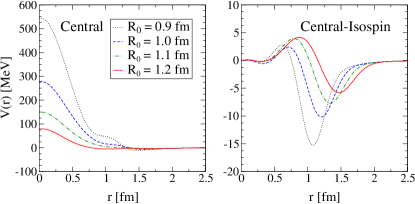
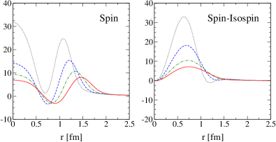
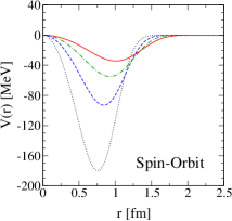
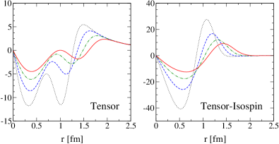
Figure 1: (Color online) Local chiral NN potentials $V(r)$ at N²LO for an SFR cutoff $\tilde{\Lambda}=1000\,\mathrm{MeV}$, decomposed into the central, central-isospin, spin, spin-isospin, spin-orbit, tensor, and tensor-isospin components, for cutoffs $R_{0}=0.9-1.2\,\mathrm{fm}$. For all components, we observe a softening of the potential going from a cutoff $R_{0}=0.9\,\mathrm{fm}$ to $R_{0}=1.2\,\mathrm{fm}$. We include the $R_{0}=0.9\,\mathrm{fm}$ potential for illustration, but as discussed in the text, will not use it in many-body calculations.

We are now in the position to specify the regularization scheme for the NN potential. Following Ref. Gezerlis:2013ipa , this is achieved by multiplying the coordinate-space expressions for the long-range potential in Eqs. (3), (4), (6)–(8), and (II)–(15) with a regulator function

$$V_{\rm long}(r)\;\to\;V_{\rm long}(r)\Big{(}1-e^{-(r/R_{0})^{4}}\Big{)}\,.$$ (29)

This ensures that short-distance parts of the long-range potentials at $r$ smaller than $R_{0}$ are smoothly cut off. For the short-range terms in Eqs. (23), (24), (27), and (28) the regularization is achieved by employing a local regulator $f_{\rm local}(q^{2})$, leading to the replacement of the $\delta$-function by a smeared one with the same exponential smearing factor as for the long-range regulator,

$$\delta({\bf r})\;\to\;\delta_{R_{0}}({\bf{r}})=\alpha e^{-(r/R_{0})^{4}}\,,$$ (30)

where the normalization constant,

$$\alpha=\frac{1}{\pi\Gamma\bigl{(}3/4\bigr{)}R_{0}^{3}}\,,$$ (31)

ensures that

$$\int d^{3}r\,\delta_{R_{0}}({\bf{r}})=1\,.$$ (32)

The Fourier transformations of the contact interactions taking into account the local regulator $f_{\rm local}(q^{2})$ are given in Appendix B. The choice of the coordinate-space cutoff $R_{0}$ is dictated by the following considerations. On the one hand, one would like to take $R_{0}$ as small as possible to ensure that one keeps most of the long-range physics associated with the pion-exchange potentials. On the other hand, it is shown in Ref. Baru:2012iv that at least for the particular class of pion-exchange diagrams corresponding to the multiple-scattering series, the chiral expansion for the NN potential breaks down at distances of the order of $r\sim 0.8\,\mathrm{fm}$ but converges fast for $r\gtrsim 1\,\mathrm{fm}$. This suggests that a useful choice of the cutoff $R_{0}$ is $R_{0}\sim 1\,\mathrm{fm}$, which corresponds to momentum-space cutoffs of the order of $\sim 500\,\mathrm{MeV}$. This follows from Fourier transforming the regulator function, integrating it from $0$ to infinity, and comparing to a sharp cutoff. These values are similar to the ones adopted in the already existing, nonlocal implementations of the chiral potential EGMN2LO ; Entem:2003ft , see also Ref. Rentmeester:1999vw ; Marji:2013uia for a related discussion.

In view of the arguments provided in Refs. Lepage:1997cs ; Epelbaum:2009sd ; Zeoli:2012bi , we will not use significantly lower values of $R_{0}$ in applications,  although we were able to obtain fits to NN phase shifts using $R_{0}=0.9\,\mathrm{fm}$. However, the LECs start to become unnatural for this cutoff. On the other hand, choosing considerably larger values of $R_{0}$ results in cutting off the long-range physics we want to preserve and, thus, introduces an unnecessary limitation in the breakdown momentum of the approach. Therefore, here and in the following, we will allow for a variation of the cutoff $R_{0}$ in the range of $R_{0}=1.0-1.2\,\mathrm{fm}$. Because the local regulator eliminates a considerable part of short-distance components of the TPE potential, we are much less sensitive to the choice of the SFR cutoff $\tilde{\Lambda}$ as compared to Refs. EGMN2LO ; Epelbaum:2003xx and can safely increase it up to $\tilde{\Lambda}=1.4$ GeV without producing spurious deeply bound states. In this work, we will vary $\tilde{\Lambda}$ in the range $\tilde{\Lambda}=1.0-1.4$ GeV. In future work, we will explore removing the SFR cutoff $\tilde{\Lambda}\to\infty$.

We would like to underline that there is no conceptual difference between our local regularization and the nonlocal regularization currently used in widely employed versions of chiral interactions in momentum space. The local chiral potentials include the same physics as the momentum-space versions. This is especially clear when antisymmetrizing. The local regulator by construction preserves the long-range parts of the interaction. When Fourier transformed, it generates higher-order q²-dependent terms when applied to short-range operators, like those already present at NLO and N²LO. Note that antisymmetrization and local regularization do not commute, but the commutator is given by higher-order terms. At NLO and N²LO, the $2+7$ contact interactions provide a most general representation consistent with all symmetries.

It remains to specify the values of the LECs and masses that enter the NN potentials at N²LO. In the following, we use $m_{p}=938.272\,\mathrm{MeV}$, $m_{n}=939.565\,\mathrm{MeV}$, the average pion mass $M_{\pi}=138.03\,\mathrm{MeV}$, the pion decay constant $F_{\pi}=92.4\,\mathrm{MeV}$, and the axial coupling $g_{A}=1.267$. For the pion-nucleon coupling, we adopt the value of $g^{2}_{\pi N}/(4\pi)=13.54$ which is consistent with Ref. Timmermans:1990tz , which also agrees with the recent determination in Ref. Baru:2010xn based on the Goldberger-Miyazawa-Oehme sum rule and utilizing the most accurate available data on the pion-nucleon scattering lengths. In order to account for the GTD as described above, we use the value $g_{A}=1.29$ in the expressions for the OPE potential. For the LECs $c_{i}$ in the N²LO TPE potential, we use the same values as in Ref. EGMN2LO , namely $c_{1}=-0.81\,\mathrm{GeV}^{-1},c_{3}=-3.4\,\mathrm{GeV}^{-1}$, and $c_{4}=3.4\,\mathrm{GeV}^{-1}$.

We emphasize that we use the same expression for the OPE potential that includes isospin-symmetry-breaking corrections and accounts for the GTD as well as the same isospin-symmetry-breaking contact interactions at all orders in the chiral expansion to allow for a more meaningful comparison between LO, NLO and N²LO.

With the NN potential specified as above, we have performed $\chi^{2}$-fits to neutron-proton phase shifts from the Nijmegen PWA Stoks:1993tb for $R_{0}=0.9$, $1.0$, $1.1$ and $1.2\,\mathrm{fm}$ and $\tilde{\Lambda}=0.8$, $1.0$, $1.2$ and $1.4$ GeV. We used the separation of spin-singlet and spin-triplet channels, and, at LO, fit the ${}^{1}S_{0}$ and ${}^{3}S_{1}$ partial waves separately while at NLO and N²LO we fit the $\{^{1}S_{0},^{1}P_{1}\}$ and $\{^{3}S_{1},\epsilon_{1},^{3}P_{0},^{3}P_{1},^{3}P_{2}\}$ partial waves. At NLO and N²LO, we used the same energies of $E_{\rm lab}=1$, $5$, $10$, $25$, $50$, $100$ and $150\,\mathrm{MeV}$ for $R_{0}=1.0$ and $R_{0}=1.1\,\mathrm{fm}$ as in the Nijmegen PWA and the errors in the phase shifts provided in Ref. Stoks:1993tb . For $R_{0}=1.2\,\mathrm{fm}$, the fits are performed up to $E_{\rm lab}=100\,\mathrm{MeV}$. At LO, the fits are performed up to $E_{\rm lab}=50\,\mathrm{MeV}$. Finally, the values of the LECs $C_{\rm CIB}$ and $C_{\rm CSB}$ are adjusted to reproduce the proton-proton ${}^{1}S_{0}$ scattering length $a_{pp}=-7.81\,\mathrm{fm}$ and the recommended value of the neutron-neutron scattering length $a_{nn}=-18.9\,\mathrm{fm}$. Note that we only take into account the point-like Coulomb force for the electromagnetic interaction as appropriate to N²LO, see Ref. EGMN2LO for more details. The resulting LECs for $R_{0}=1.0,1.1,1.2\,\mathrm{fm}$ and $\tilde{\Lambda}=1000\,\mathrm{MeV}$ are shown in Table 1 and for $\tilde{\Lambda}=1400\,\mathrm{MeV}$ in Table 2.

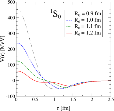
Figure 2: (Color online) Local chiral NN potentials $V(r)$ at N²LO for an SFR cutoff $\tilde{\Lambda}=1000\,\mathrm{MeV}$ in the ${}^{1}S_{0}$ partial wave in the neutron-neutron system.

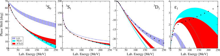
Figure 3: (Color online) Phase shifts for the ${}^{1}S_{0}$ and ${}^{3}S_{1}-^{3}D_{1}$ partial waves at LO, NLO, and N²LO in comparison with the Nijmegen partial wave analysis (PWA) Stoks:1993tb . The bands at each order correspond to the cutoff variation of $R_{0}=1.0-1.2\,\mathrm{fm}$. At NLO and N²LO, we also vary the SFR cutoff from $\tilde{\Lambda}=1.0-1.4\,\mathrm{GeV}$.

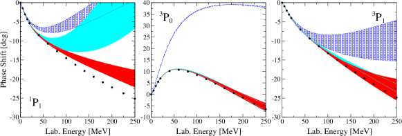
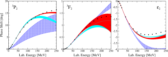
Figure 4: (Color online) Phase shifts for the ${}^{1}P_{1}$, ${}^{3}P_{0}$, ${}^{3}P_{1}$ and ${}^{3}P_{2}$$-$${}^{3}F_{2}$ partial waves at LO, NLO, and N²LO in comparison with the Nijmegen PWA Stoks:1993tb . The bands are obtained as in Fig. 3.

It would be useful to have a quantitative comparison of different fits, e.g., comparing the local chiral potentials presented here with the nonlocal optimized N²LO potentials of Refs. Ekstrom:2013 ; Ekstrom:2014 or with the analyses of Refs. NavarroPerez:2014 ; NavarroPerez:2014b . One possibility would be to calculate the $\chi^{2}$/datum, but unfortunately we presently do not have the machinery to do this. We also emphasize that our fitting strategy is different to the nonlocal optimized N²LO potentials. As discussed, we only fit at low energies and take the $c_{i}$’s from pion-nucleon scattering, whereas the optimized N²LO potentials fit these over the full energy range considered.

The fits are different from the fits used in Ref. Gezerlis:2013ipa because our previous fitting routine was incorrect in the tensor channel of the pion-exchange interactions. This error has only a small influence in pure neutron matter.

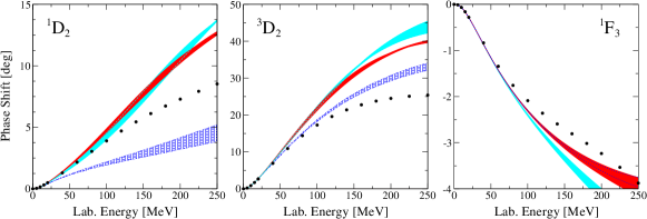
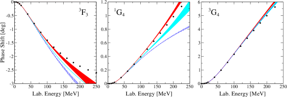
Figure 5: (Color online) Phase shifts for the ${}^{1}D_{2}$, ${}^{3}D_{2}$, ${}^{1}F_{3}$, ${}^{3}F_{3}$, ${}^{1}G_{4}$, and ${}^{3}G_{4}$ partial waves at LO, NLO, and N²LO in comparison with the Nijmegen PWA Stoks:1993tb . The bands are obtained as in Fig. 3.

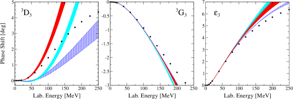
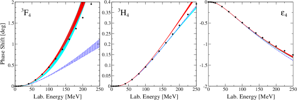
Figure 6: (Color online) Phase shifts for the ${}^{3}D_{3}$$-$${}^{3}G_{3}$ and ${}^{3}F_{4}$$-$${}^{3}H_{4}$ partial waves at LO, NLO, and N²LO in comparison with the Nijmegen PWA Stoks:1993tb . The bands are obtained in the same way as in Fig. 3.

In Fig. 1, we show the local chiral potentials $V(r)$ at N²LO for a SFR cutoff $\tilde{\Lambda}=1000\,\mathrm{MeV}$, decomposed into the central, central-isospin, spin, spin-isospin, spin-orbit, tensor, and tensor-isospin components

$$V(r) =V^{\text{central}}(r)+V^{\text{central-isospin}}(r)\,\,\mbox{\boldmath$\tau$}_{1}\cdot\mbox{\boldmath$\tau$}_{2}$$

$$\quad+\left[V^{\text{spin}}(r)+V^{\text{spin-isospin}}(r)\,\,\mbox{\boldmath$\tau$}_{1}\cdot\mbox{\boldmath$\tau$}_{2}\right]\mbox{\boldmath$\sigma$}_{1}\cdot\mbox{\boldmath$\sigma$}_{2}$$

$$\quad+V^{\text{LS}}(r)\,\,{\bf{L}}\cdot{\bf{S}}$$

$$\quad+\left[V^{\text{tensor}}(r)+V^{\text{tensor-isospin}}(r)\mbox{\boldmath$\tau$}_{1}\cdot\mbox{\boldmath$\tau$}_{2}\right]S_{12}(r)\,,$$ (33)

for cutoffs $R_{0}=0.9-1.2\,\mathrm{fm}$. We include the $0.9\,\mathrm{fm}$ potential for illustration, but we do not recommend it for many-body calculations and therefore do not include it in our own calculations or in the tables. For all components we see a softening of the potential going from $R_{0}=0.9\,\mathrm{fm}$ to $R_{0}=1.2\,\mathrm{fm}$, as expected, because short-range parts of the potentials are strongly scheme dependent. The structures in the individual channels are due to adding up different contributions to those channels with different $r$-dependencies.

In addition, we show the local chiral potentials $V(r)$ at N²LO for a SFR cutoff $\tilde{\Lambda}=1000\,\mathrm{MeV}$ in the ${}^{1}S_{0}$ channel in Fig. 2 in the neutron-neutron system. Again, we observe a softening of the potential when increasing the coordinate space cutoff from $R_{0}=0.9\,\mathrm{fm}$ to $R_{0}=1.2\,\mathrm{fm}$.

Table 3: Deuteron properties for the local chiral potentials at LO, NLO, and N²LO. We tabulate the deuteron binding energy $E_{d}$, the $D$-state probability $P_{D}$, the magnetic moment $\mu_{d}$, the quadrupole moment $Q_{d}$, the asymptotic D/S ratio $\eta$, the asymptotic $S$-wave factor $A_{s}$, and the rms radius $r_{d}$. The ranges include a cutoff variation $R_{0}=1.0-1.2\,\mathrm{fm}$ and, at NLO and N²LO, a variation of the SFR cutoff $\tilde{\Lambda}=1.0-1.4\,\mathrm{GeV}$. The experimental results are taken from Refs. Deuteron:Eb ; Deuteron:mud ; Deuteron:Qd ; Deuteron:eta ; Deuteron:rd ; Deuteron:AS . We compare our results with the N²LO EGM results of Ref. EGMN2LO , where the cutoff variation is $\Lambda=450-650\,\mathrm{MeV}$ and $\tilde{\Lambda}=500-700\,\mathrm{MeV}$.

	LO	NLO	N2LO	N2LO EGM	Exp.
$E_{d}[\,\mathrm{MeV}]$	$-2.0243\ldots-2.0161$	$-2.1597\ldots-2.1446$	$-2.2177\ldots-2.1981$	$-2.202\ldots-2.189$	$-2.225$
$P_{D}[\%]$	$4.2761\ldots 5.3356$	$6.9249\ldots 8.1702$	$5.5059\ldots 6.1356$	$3.53\ldots 4.93$
$\mu_{d}[\mu_{N}]$	$0.8494\ldots 0.8554$	$0.8332\ldots 0.8403$	$0.8438\ldots 0.8484$		$0.857$
$Q_{d}[\,\mathrm{fm}^{2}]$	$0.2580\ldots 0.2691$	$0.3013\ldots 0.3039$	$0.2828\ldots 0.2890$	$0.271\ldots 0.275$	$0.286$
$\eta$	$0.0232\ldots 0.0240$	$0.0275\ldots 0.0278$	$0.0256\ldots 0.0267$	$0.0255\ldots 0.0256$	$0.0256$
$A_{s}[\,\mathrm{fm}^{-\frac{1}{2}}]$	$0.8299\ldots 0.8321$	$0.8605\ldots 0.8648$	$0.8765\ldots 0.8818$	$0.874\ldots 0.879$	$0.885$
$r_{d}[\,\mathrm{fm}]$	$1.9897\ldots 1.9919$	$1.9737\ldots 1.9758$	$1.9677\ldots 1.9698$	$1.970\ldots 1.972$	$1.966$

III Phase shifts

Next, we present the neutron-proton phase shifts in partial waves up to $J=4$ for the local chiral potentials at LO, NLO, and N²LO for laboratory energies up to $250\,\mathrm{MeV}$ in comparison with the Nijmegen PWA Stoks:1993tb . We vary the cutoff between $R_{0}=1.0-1.2\,\mathrm{fm}$ and, at NLO and N²LO, the SFR cutoff between $\tilde{\Lambda}=1.0-1.4\,\mathrm{GeV}$.

In Fig. 3, we show the ${}^{1}S_{0}$ phase shifts as well as the ${}^{3}S_{1}-^{3}D_{1}$ coupled channel. The description of the ${}^{1}S_{0}$ channel at LO is only good at very low energies and improves when going to NLO and the effective range physics is included. When going from NLO to N²LO, the cutoff bands overlap. In the ${}^{3}S_{1}$ channel the situation is similar but the cutoff bands are narrower. In both $S$-wave channels the width of the bands at NLO and N²LO are of similar size. This is due to the truncation of the short-range contact interactions and the large $c_{i}$ couplings entering at N²LO, and is visible in all phase shifts.

In the ${}^{3}D_{1}$ channel the description worsens when going from LO to NLO and improves only slightly from NLO to N²LO. At N²LO the description of the ${}^{3}D_{1}$ channel is poor for energies larger than $50\,\mathrm{MeV}$. In addition, also the description of the $J=1$ mixing angle is poor at all orders, a fact which is clearly reflected in the size of the cutoff bands.

In Fig. 4 we show the phase shifts for the $P$ waves and the $J=2$ coupled channel. In the ${}^{1}P_{1}$ channel the LO band starts to deviate from the data already at low energies. Including additional spin-orbit and tensor contributions at NLO improves the description of the ${}^{1}P_{1}$ channel only little. However, the situation highly improves when going to N²LO.

In the ${}^{3}P$ waves the phase shifts improve considerably going from LO to higher orders and the description of the ${}^{3}P$ waves at N²LO is substantially better than in our previous fits Gezerlis:2013ipa . Furthermore, the description of the $J=2$ coupled channel is considerably better than for the $J=1$ coupled channel and improves when going from LO to N²LO.

In Fig. 5 we show the phase shifts for the remaining uncoupled partial waves up to $J=4$. The description of the individual channels is good even at high energies except for the $D$ waves. This can also be seen in Fig. 6 where we show the $J=3$ and $J=4$ coupled channels.

In general, the description of all $D$ wave channels is poor up to N²LO and does not improve when going from NLO to N²LO. This is due to the truncation of the contact interactions at N²LO because in partial waves with orbital angular momentum $L>1$ no contact interactions contribute at this order except for regulator effects. Thus, the $D$ wave phase shifts are described almost solely by pion-exchange interactions and are parameter free. This can be improved by going to N³LO. The higher $L>2$ partial waves instead are mostly described by long-range pion-exchange interactions and already the OPE interaction at LO describes the data well at low energies. Thus, the higher partial waves can be well described already at N²LO.

Comparing our phase shift results to the results obtained with the nonlocal N²LO momentum space potential of Ref. EGMN2LO , we find that the local potentials describe all partial waves up to $J=4$ better except for the $D$ waves. In addition, the cutoff variation is smaller for the local chiral potentials.

IV Deuteron

In this section, we calculate deuteron properties using the local chiral potentials presented in the previous sections at LO, NLO, and N²LO. We calculate the deuteron binding energy $E_{d}$, the quadrupole moment $Q_{d}$, the magnetic moment $\mu_{d}$, the asymptotic D/S ratio $\eta$, the root-mean-square (rms) radius $r_{d}$, the asymptotic $S$-wave factor $A_{s}$, and the $D$-state probability $P_{D}$. We vary the cutoff $R_{0}=1.0-1.2\,\mathrm{fm}$ and, at NLO and N²LO, the SFR cutoff $\tilde{\Lambda}=1.0-1.4\,\mathrm{GeV}$. The deuteron properties are calculated as described in Ref. EGMN2LO . The results are shown in Table 3 and are compared with experimental results of Refs. Deuteron:Eb ; Deuteron:mud ; Deuteron:Qd ; Deuteron:eta ; Deuteron:rd ; Deuteron:AS and the N²LO Epelbaum, Glöckle, and Meißner (EGM) results of Ref. EGMN2LO , where the cutoff variation is $\Lambda=450-650\,\mathrm{MeV}$ and $\tilde{\Lambda}=500-700\,\mathrm{MeV}$.

At N²LO we find a deuteron binding energy of $-2.208\pm 0.010\,\mathrm{MeV}$, which has to be compared with the experimental value of $-2.225\,\mathrm{MeV}$. Thus, the N²LO result deviates from the experimental result by less than $1\%$, which is better than $2.196\pm 0.007$ for the nonlocal, momentum-space N²LO EGM potentials of Ref. EGMN2LO . However, for those potentials the range of the cutoff variation is different, which affects the results and theoretical error estimates.

The description of the deuteron quadrupole moment is surprisingly good for the local chiral potentials and the experimental result lies within the N²LO uncertainty band. Note that electromagnetic two-body currents are not included. The results for the N²LO momentum space potentials instead deviate by $4-5\%$. Also for the other observables the result of the local N²LO potentials deviates less than $1\%$ from the experimental values.

V QMC calculations of
neutron matter

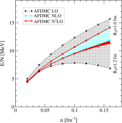
Figure 7: (Color online) Neutron matter energy per particle $E/N$ as a function of density $n$ using AFDMC with the local chiral NN potentials at LO, NLO, and N²LO. The bands are obtained by varying the cutoff $R_{0}=1.0-1.2\,\mathrm{fm}$ and the SFR cutoff $\tilde{\Lambda}=1000-1400\,\mathrm{MeV}$.

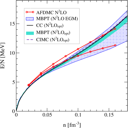
Figure 8: (Color online) Neutron matter energy per particle $E/N$ as a function of density $n$. We compare our AFDMC N²LO results of this work with the MBPT N²LO results of Ref. Tews:2013 using the momentum-space potentials of Ref. EGMN2LO , the coupled-cluster results of Ref. Hagen:2014 using the optimized N²LO potential of Ref. Ekstrom:2013 , the MBPT results of Ref. Tews:2013b , and the configuration interaction Monte Carlo (CIMC) results of Ref. Roggero:2014 , both using the same optimized N²LO potential.

Local chiral EFT interactions can be used in any modern many-body method. This includes Quantum Monte Carlo. The two main methods in the context of nuclear physics are GFMC, which is very accurate but also computationally costly, and AFDMC, which is computationally less costly at the price of less accuracy. Up to now, nuclear GFMC calculations have used phenomenological NN interactions as input, typically of the Argonne family Wiringa1995 ; Wiringa2002 . These potentials are accurate, but are not connected to an EFT of QCD and their two-pion exchange interaction is modeled rather phenomenologically, which makes it difficult to construct consistent 3N forces. Thus, it will be key to use the new local potentials in light nuclei GFMC calculations, work that is currently ongoing Lynn2014 .

In this paper, we use the new local chiral potentials in AFDMC calculations for pure neutron matter and expand on our first results of Ref. Gezerlis:2013ipa . For technical reasons, in the past it has not been possible to extend AFDMC to realistic potentials when both neutrons and protons are involved. However, for pure neutron matter, either in the homogeneous case or in a confining potential, the situation is more straightforward and AFDMC compares favorably with the more accurate nuclear GFMC results Gandolfi:2011 ; Carlson:2003 . Neutron matter is useful as a test case in which different aspects of nuclear interactions can be probed, but is also directly relevant to the properties of neutron stars and as ab initio input to energy density functionals Gandolfi:2011 ; Gandolfi:2012 ; Gezerlis:2008 ; Chamel:2008 ; Hebeler:2010b ; nstar_long .

In Fig. 7, we show AFDMC results for 66 neutrons for the local chiral potentials at LO, NLO, and N²LO, varying $R_{0}=1.0-1.2\,\mathrm{fm}$, corresponding to a cutoff range of $\sim 500-400\,\mathrm{MeV}$ in momentum space, and the SFR cutoff $\tilde{\Lambda}=1000-1400\,\mathrm{MeV}$. At all these orders the $R_{0}=1.1\,\mathrm{fm}$ results lie between the $R_{0}=1.0\,\mathrm{fm}$ and $R_{0}=1.2\,\mathrm{fm}$ ones. This can also be seen in more detail in Fig. 11, where we show the AFDMC results individually for three different regulators $R_{0}=1.0\,\mathrm{fm},1.1\,\mathrm{fm},$ and $1.2\,\mathrm{fm}$ and a SFR cutoff of $\tilde{\Lambda}=1000\,\mathrm{MeV}$, along with the many-body perturbation theory results that will be discussed in the next section.

As shown in Ref. Gezerlis:2013ipa , the LO results lead to a broad band, the lower part of which ($R_{0}=1.2\,\mathrm{fm}$) even changes slope as the density is increased. This reflects the fact that the LO potential does not describe the phase shifts at the relevant energies as there are only two LECs at this order. The NLO and N²LO results are generally similar in size, as observed in Ref. Gezerlis:2013ipa , due to the large $c_{i}$ entering at N²LO and the same truncation of the contact interactions at both orders. The width of these bands is similar to that of the phase shifts discussed in Sect. III.

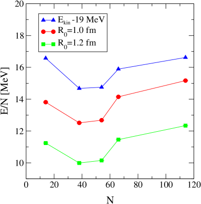
Figure 9: (Color online) Finite-size effects for the ground-state energy of neutron matter for a SFR cutoff $\tilde{\Lambda}=1000\,\mathrm{MeV}$ at N²LO. Results are shown for different particle numbers for the $R_{0}=1.0\,\mathrm{fm}$ and the $R_{0}=1.2\,\mathrm{fm}$ potentials. We also show the kinetic energy, shifted down by $19\,\mathrm{MeV}$. The finite-size effects for the local chiral potentials follow the shell effects of the kinetic energy operator.

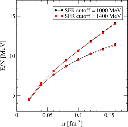
Figure 10: (Color online) Ground-state energy of 66 neutrons at N²LO. Shown are results for two SFR cutoffs, $\tilde{\Lambda}=1000\,\mathrm{MeV}$ and $\tilde{\Lambda}=1400\,\mathrm{MeV}$, and two different cutoffs $R_{0}=1.0\,\mathrm{fm}$ (upper lines) and $R_{0}=1.2\,\mathrm{fm}$ (lower lines). The results exhibit a very weak $\tilde{\Lambda}$ dependence.

In Ref. Gezerlis:2013ipa , we varied the cutoff from $R_{0}=0.8\,\mathrm{fm}$ to $R_{0}=1.2\,\mathrm{fm}$. Since we have been unable to produce a precision potential with no deeply bound states for $R_{0}=0.8\,\mathrm{fm}$, we cannot directly compare our new AFDMC results with those of Ref. Gezerlis:2013ipa , because the latter had an error in the fitting routine for the tensor channel of the pion-exchange interactions, which however only has a small effect on pure neutron matter. The narrower range of cutoff variation in this work has made the bands somewhat smaller, at $0.15\,\mathrm{fm}^{-3}$, the range is $8.1\,\mathrm{MeV}$ at LO, $2.1\,\mathrm{MeV}$ at NLO, and $2.1\,\mathrm{MeV}$ at N²LO.

In Fig. 8 we compare our AFDMC N²LO results for neutron matter with the MBPT N²LO calculation of Ref. Tews:2013 based on the momentum-space potentials of Ref. EGMN2LO , the coupled-cluster results of Ref. Hagen:2014 using the optimized N²LO potential of Ref. Ekstrom:2013 , the MBPT results of Ref. Tews:2013b , and the CIMC calculation of Ref. Roggero:2014 , both using the same optimized N²LO potential. The bands for the MBPT results are obtained as described in Ref. Tews:2013 .

The different many-body results for the optimized N²LO potential are in very good agreement. These results also agree very well with recent self-consistent Green’s function results Carbone:2014 . In addition, the optimized N²LO results agree very well with the N²LO band of Ref. Tews:2013 which includes also a NN cutoff variation and is therefore rather broad. Comparing with the AFDMC results of this paper, we find that at saturation density the resulting energies per particle agree very well. However, the general density dependence of the AFDMC results is more flat, leading to higher energies at intermediate densities and a different density dependence at saturation density. These differences could be due to the differences in the phase shift predictions, and we expect both results to come closer when going to N³LO.

We have also tested the dependence of the AFDMC results on the Jastrow term in the variational wave function. Specifically, the trial wave function in AFDMC is written as

$$\Psi_{T}(\mathbf{R},\mathbf{S})={\cal A}\left[\prod_{i}\phi_{\alpha}(\mathbf{r}_{i},s_{i})\right]\prod_{i<j}f(r_{ij})\,,$$ (34)

where $\alpha$ labels the single-particle state. For a nodeless Jastrow term, most QMC methods are independent of the choice one makes for $f(r)$: the Jastrow function impacts the statistical error bar by accenting the “appropriate” regions of phase space, but not the value itself. However, due to the complicated spin-dependence of nuclear interactions, it has been found that AFDMC has a small dependence on the Jastrow function as reported in Ref. Gezerlis:2013ipa . By comparing AFDMC results for 14 particles using the Argonne family of potentials with a GFMC calculation for the same potentials and neutron number (the largest neutron number for which GFMC results exist), we found that the Jastrow dependence disappears in AFDMC when using a softened Jastrow function.

Because no GFMC results exist for 66 particles, we have carried out separate computations at the highest density considered here ($n=0.16\,\mathrm{fm}^{-3}$). We studied Jastrow terms from solving the Schrödinger equation for the Argonne $v_{8}^{\prime}$ potential, a typical QMC potential of reference, and from the consistent local chiral potentials. In addition, we have examined the effect of artificially softening the Jastrow term by multiplying the input potential (only when producing the Jastrow function) by a fixed coefficient, in order to see the effect of removing the Jastrow. The highest energies always result from using a largely unmodified Argonne $v_{8}^{\prime}$ potential, as this is the potential that is most different from the new chiral interactions. In the case of $R_{0}=1.0\,\mathrm{fm}$ the different Jastrow terms lead to an energy per particle that varies by at most 0.1 MeV at $0.16\,\mathrm{fm}^{-3}$, while for the $R_{0}=1.2\,\mathrm{fm}$ potentials the variation is 0.15 MeV. Both these results are much smaller than the $0.6\,\mathrm{MeV}$ quoted in Ref. Gezerlis:2013ipa for the $R_{0}=0.8\,\mathrm{fm}$ potential. This is a reflection of the softer potentials in the present work.

Furthermore, we have probed in detail the finite-size effects for the local chiral potentials. As we are interested in describing the thermodynamic limit of neutron matter, it is important that we are using sufficiently many particles in our AFDMC simulations. In order to avoid issues related to preferred directions in momentum-space, we have performed calculations for closed shells: $N=14$, 38, 54, 66, 114. We chose the SFR cutoff $\tilde{\Lambda}=1000\,\mathrm{MeV}$ and performed simulations at N²LO for both the $R_{0}=1.0\,\mathrm{fm}$ and $R_{0}=1.2\,\mathrm{fm}$ potentials at the highest density $n=0.16\,\mathrm{fm}^{-3}$. The results are shown in Fig. 9. We observe that the two potentials exhibit essentially identical shell structure, as was to be expected because the ranges involved in the two potentials are basically the same. These results show a dependence on $N$ that is very similar to that in Table III of Ref. Gandolfi:2009 for the values of $N$ used in that reference, namely 14, 38, and 66. The shell structure is very similar to that of the free Fermi gas in a periodic box, which we also show in Fig. 9. From the free Fermi gas we expect that the thermodynamic limit value is below the $N=114$ result and very close to the $N=66$ value. This justifies our choice of using 66 particles to simulate the thermodynamic limit. The only qualitative difference between the free Fermi-gas shell structure and our AFDMC results appears at $N=14$. For the free gas $N=14$ leads to an energy that is higher than that at $N=66$. This results from the very small periodic box needed to produce the same density for $N=14$. In that case the interaction length scales also start to be important. In contrast, for larger $N$, shell effects come almost completely from the kinetic energy behavior.

We have also explored the dependence of the results on different values of the SFR cutoff. As discussed, the effect of the SFR cutoff $\tilde{\Lambda}$ is expected to be smaller than that of $R_{0}$. We show the results of varying the SFR cutoff from $\tilde{\Lambda}=1000$ MeV to $\tilde{\Lambda}=1400$ MeV for $R_{0}=1.0\,\mathrm{fm}$ and $R_{0}=1.2\,\mathrm{fm}$ in Fig. 10. There is essentially no effect at low densities, while at higher densities the difference for $R_{0}=1.0\,\mathrm{fm}$ never exceeds 0.1 MeV and for $R_{0}=1.2\,\mathrm{fm}$ it is always less than 0.15 MeV. This shows that the SFR cutoff has a negligible impact on the many-body results.

VI Perturbative calculations of
neutron matter

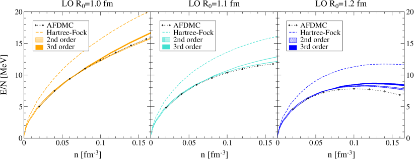
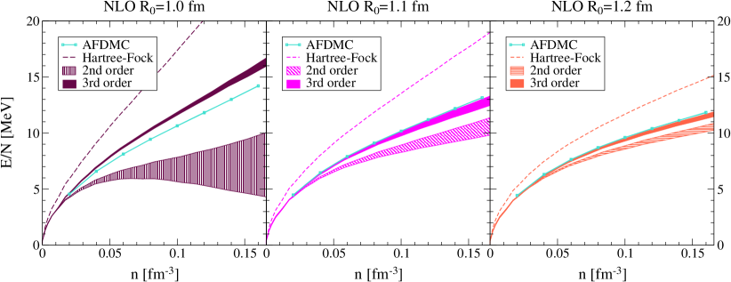
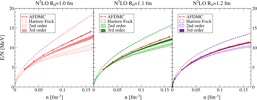
Figure 11: (Color online) Results for MBPT and AFDMC calculations at LO, NLO, and N²LO for $R_{0}=1.0-1.2\,\mathrm{fm}$. For the MBPT results, we show the Hartree-Fock energies as well as the energy at second order and including third-order particle-particle and hole-hole corrections. The width of the bands includes a variation of the single-particle spectrum from a free to a Hartree-Fock spectrum. In addition, for both the MBPT and AFDMC results we also vary the SFR cutoff $\tilde{\Lambda}=1000-1400\,\mathrm{MeV}$. For the LO $1.1\,\mathrm{fm}$ results, the lower band corresponds to the second-order results.

We have also performed neutron matter calculations using many-body perturbation theory (following Refs. Hebeler:2010a ; nucmatt ; Tews:2013 ; Kruger:2013 ) for the same local chiral potentials and the same regulators as in the previous section. We show the results in Fig. 11 together with the AFDMC results at LO, NLO, and N²LO for the three different cutoffs $R_{0}=1.0,1.1,$ and $1.2\,\mathrm{fm}$, and varying the SFR cutoff $\tilde{\Lambda}=1000-1400\,\mathrm{MeV}$.

At every order in the chiral expansion and for every cutoff we show the results at the Hartree-Fock level as a dashed line, including second-order contributions as a shaded band, and including also third-order particle-particle and hole-hole corrections as solid bands. The bands are obtained by employing a free or Hartree-Fock single-particle spectrum and by varying the SFR cutoff as stated above. Again, we observe that the $R_{0}=1.1\,\mathrm{fm}$ results at all three chiral orders lie between the $R_{0}=1.0\,\mathrm{fm}$ and $R_{0}=1.2\,\mathrm{fm}$ ones.

At LO, the local chiral potentials in general follow the trend of the AFDMC results for all three cutoffs. The width of the individual bands is very small and the energy changes from first to second and from second to third order are small. As discussed in Ref. Kruger:2013 , this energy difference, combined with the weak dependence on the different single-particle spectra, is a measure of the perturbative convergence for the individual potentials. All potentials at this chiral order seem to be perturbative. We find a good agreement between the AFDMC and the MBPT results, especially at lower densities, although at higher densities the trend is that the second-order results are better than third-order.

At NLO, we find the $R_{0}=1.0\,\mathrm{fm}$ potential to have the slowest, if any, perturbative convergence. The second-order band is very broad and the third-order contributions are large: at saturation density they are $6-10\,\mathrm{MeV}$. Going to higher coordinate-space cutoffs, which means lower momentum cutoffs, we find that the potential becomes more perturbative. At $R_{0}=1.2\,\mathrm{fm}$ both the second- and third-order bands are narrow and the third-order contributions are $\approx 1.5\,\mathrm{MeV}$.

At N²LO the results are very similar to NLO. We find that the $R_{0}=1.0\,\mathrm{fm}$ potential shows the slowest perturbative convergence, with an energy difference from second to third order of about $3\,\mathrm{MeV}$ at saturation density. However, the perturbativeness for this cutoff at N²LO is better than at NLO. Going to higher coordinate-space cutoffs again improves the perturbativeness and for $R_{0}=1.2\,\mathrm{fm}$ the energy difference is $\approx 1.0\,\mathrm{MeV}$ at this density. This behavior is similar to the nonlocal potentials used in Ref. Kruger:2013 where it was shown that soft (low momentum cutoff) potentials have a better convergence.

For the perturbative $R_{0}=1.2\,\mathrm{fm}$ potentials, the agreement between the third-order perturbative results and the AFDMC results is excellent. For $R_{0}=1.2\,\mathrm{fm}$, at N²LO, the perturbative results lie almost on top of the AFDMC values. The difference between the third-order result with Hartree-Fock single-particle spectrum and the AFDMC results is $0.2\,\mathrm{MeV}$ at $0.16\,\mathrm{fm}^{-3}$ for $\tilde{\Lambda}=1400\,\mathrm{MeV}$ and only $20\,\mathrm{keV}$ for $\tilde{\Lambda}=1000\,\mathrm{MeV}$. In comparison, at NLO the difference is $0.2\,\mathrm{MeV}$ at $0.16\,\mathrm{fm}^{-3}$ for $\tilde{\Lambda}=1400\,\mathrm{MeV}$ and $0.1\,\mathrm{MeV}$ for $\tilde{\Lambda}=1000\,\mathrm{MeV}$, while at LO it is $1.6\,\mathrm{MeV}$. These results constitute a direct validation of MBPT for neutron matter based on low momentum potentials, in this case $R_{0}=1.1\,\mathrm{fm}$ and $R_{0}=1.2\,\mathrm{fm}$, which was the main finding in our initial QMC study with chiral EFT interactions Gezerlis:2013ipa .

VII Summary and Outlook

We have presented details of the derivation of local chiral EFT potentials at LO, NLO, and N²LO. We performed fits of the LECs to low-energy NN phase shifts, which are well reproduced in most cases, and agree better than for the momentum-space potentials with the Nijmegen PWA. Furthermore, the calculated deuteron properties at N²LO show very good agreement with experimental data.

We have applied the new local chiral potentials to neutron matter using AFDMC and MBPT. In particular, we have investigated the sensitivity of the results to the local regulator and to the SFR cutoff, to the influence of the Jastrow term, and also to finite size effects in AFDMC.

The excellent agreement of the results for the softer $R_{0}=1.1\,\mathrm{fm}$ and $R_{0}=1.2\,\mathrm{fm}$ potentials within the two many-body frameworks represents a direct validation of MBPT for neutron matter and will enable novel many-body calculations of nuclei and matter within QMC based on chiral EFT interactions.

Appendix A
Partial-wave-decomposed contact interactions

We fit the LECs $C_{S},C_{T},$ and $C_{1-7}$ to NN phase shifts. In every partial wave only certain LECs contribute. In the following we give the partial wave decomposition for all relevant channels. We use spectroscopic LECs given in terms of $C_{S},C_{T},$ and $C_{1-7}$ as follows:

$$d_{11} =C_{S}+C_{T}\,,$$

$$d_{22} =C_{S}-3C_{T}\,,$$

$$d_{1} =C_{1}-3C_{2}+C_{3}-3C_{4}\,,$$

$$d_{2} =C_{6}-3C_{7}\,,$$

$$d_{3} =C_{1}+C_{2}-3C_{3}-3C_{4}\,,$$

$$d_{4} =C_{1}+C_{2}+C_{3}+C_{4}\,,$$

$$d_{5} =C_{1}-3C_{2}-3C_{3}+9C_{4}\,,$$

$$d_{6} =\frac{1}{2}C_{5}\,,$$

$$d_{7} =C_{6}+C_{7}\,.$$

For the partial-wave-decomposed matrix elements we find

$$\left\langle{}^{1}S_{0}\right|V_{\text{cont}}\left|{}^{1}S_{0}\right\rangle =d_{22}\delta_{R_{0}}+(d_{3}-d_{7})\,20\frac{r^{2}}{R_{0}^{4}}\delta_{R_{0}}$$

$$\quad-(d_{3}-d_{7})\,16\frac{r^{6}}{R_{0}^{8}}\delta_{R_{0}}\,,$$ (35)

$$\left\langle{}^{3}S_{1}\right|V_{\text{cont}}\left|{}^{3}S_{1}\right\rangle =d_{11}\delta_{R_{0}}+(d_{1}+\frac{1}{3}d_{2})\,20\frac{r^{2}}{R_{0}^{4}}\delta_{R_{0}}$$

$$\quad-(d_{1}+\frac{1}{3}d_{2})\,16\frac{r^{6}}{R_{0}^{8}}\delta_{R_{0}}\,,$$ (36)

$$\left\langle{}^{3}S_{1}\right|V_{\text{cont}}\left|{}^{3}D_{1}\right\rangle =\left\langle{}^{3}D_{1}\right|V_{\text{cont}}\left|{}^{3}S_{1}\right\rangle$$ (37)

$$=d_{2}\frac{\sqrt{8}}{3}\,8\frac{r^{2}}{R_{0}^{4}}\delta_{R_{0}}-d_{2}\frac{\sqrt{8}}{3}\,16\frac{r^{6}}{R_{0}^{8}}\delta_{R_{0}}\,,$$

$$\left\langle{}^{3}D_{1}\right|V_{\text{cont}}\left|{}^{3}D_{1}\right\rangle =d_{11}\delta_{R_{0}}-(d_{1}-\frac{1}{3}d_{2})\,16\frac{r^{6}}{R_{0}^{8}}\delta_{R_{0}}$$

$$\quad+(d_{1}+\frac{3}{5}d_{6}+\frac{1}{15}d_{2})\,20\frac{r^{2}}{R_{0}^{4}}\delta_{R_{0}}\,,$$ (38)

$$\left\langle{}^{1}P_{1}\right|V_{\text{cont}}\left|{}^{1}P_{1}\right\rangle =\,d_{22}\delta_{R_{0}}+(d_{5}-d_{2})\,20\frac{r^{2}}{R_{0}^{4}}\delta_{R_{0}}$$

$$\quad-(d_{5}-d_{2})\,16\frac{r^{6}}{R_{0}^{8}}\delta_{R_{0}}\,,$$ (39)

$$\left\langle{}^{3}P_{0}\right|V_{\text{cont}}\left|{}^{3}P_{0}\right\rangle =d_{11}\delta_{R_{0}}-(d_{4}-d_{7})\,16\frac{r^{6}}{R_{0}^{8}}\delta_{R_{0}}$$

$$\quad+(d_{4}+\frac{2}{5}d_{6}-\frac{1}{5}d_{7})\,20\frac{r^{2}}{R_{0}^{4}}\delta_{R_{0}}\,,$$ (40)

$$\left\langle{}^{3}P_{1}\right|V_{\text{cont}}\left|{}^{3}P_{1}\right\rangle =d_{11}\delta_{R_{0}}-(d_{4}+d_{7})\,16\frac{r^{6}}{R_{0}^{8}}\delta_{R_{0}}$$

$$\quad+(d_{4}+\frac{1}{5}d_{6}+\frac{3}{5}d_{7})\,20\frac{r^{2}}{R_{0}^{4}}\delta_{R_{0}}\,,$$ (41)

$$\left\langle{}^{3}P_{2}\right|V_{\text{cont}}\left|{}^{3}P_{2}\right\rangle =d_{11}\delta_{R_{0}}-(d_{4}+\frac{1}{5}d_{7})\,16\frac{r^{6}}{R_{0}^{8}}\delta_{R_{0}}$$

$$\quad+(d_{4}-\frac{1}{5}d_{6}+\frac{7}{25}d_{7})\,20\frac{r^{2}}{R_{0}^{4}}\delta_{R_{0}}\,,$$ (42)

$$\left\langle{}^{3}P_{2}\right|V_{\text{cont}}\left|{}^{3}F_{2}\right\rangle =\left\langle{}^{3}F_{2}\right|V_{\text{cont}}\left|{}^{3}P_{2}\right\rangle$$ (43)

$$=\,d_{7}\sqrt{6}\frac{16}{5}\frac{r^{2}}{R_{0}^{4}}\delta_{R_{0}}-d_{7}\sqrt{6}\frac{32}{5}\frac{r^{6}}{R_{0}^{8}}\delta_{R_{0}}\,,$$

$$\left\langle{}^{3}F_{2}\right|V_{\text{cont}}\left|{}^{3}F_{2}\right\rangle =d_{11}\delta_{R_{0}}-(d_{4}-\frac{1}{5}d_{7})\,16\frac{r^{6}}{R_{0}^{8}}\delta_{R_{0}}$$

$$\quad+(d_{4}+\frac{4}{5}d_{6}+\frac{3}{25}d_{7})\,20\frac{r^{2}}{R_{0}^{4}}\delta_{R_{0}}\,.$$ (44)

Appendix B Fourier transformation of
contact interactions

In the following we give the Fourier transformation of the contact contributions. The LO contacts are momentum independent and their Fourier transformation is given by

$$\quad\int\!\!\!\frac{d^{3}q}{(2\pi)^{3}}\,V_{\text{cont}}^{\text{LO}}f_{\text{local}}(q^{2})e^{i\bf{q}\cdot\bf{r}}$$ (45)

$$=V_{\text{cont}}^{\text{LO}}\,\int\!\!\!\frac{d^{3}q}{(2\pi)^{3}}f_{\text{local}}(q^{2})e^{i\bf{q}\cdot\bf{r}}=V_{\text{cont}}^{\text{LO}}\,\delta_{R_{0}}({\bf r})\,,$$

where $f_{\text{local}}(q^{2})$ is a local momentum space regulator.

The first four NLO contact interactions are proportional to $q^{2}$ and contain spin and isospin operators which are not dotted into momentum operators. Writing the $q^{2}$ dependence explicitly, the Fourier transformation is given by

$$\quad\int\!\!\!\frac{d^{3}q}{(2\pi)^{3}}\,V_{\text{cont}}^{\text{NLO}}q^{2}f_{\text{local}}(q^{2})e^{i\bf{q}\cdot\bf{r}}$$ (46)

$$=-V_{\text{cont}}^{\text{NLO}}\Delta\,\int\!\!\!\frac{d^{3}q}{(2\pi)^{3}}f_{\text{local}}(q^{2})e^{i\bf{q}\cdot\bf{r}}=-V_{\text{cont}}^{\text{NLO}}\Delta\,\delta_{R_{0}}({\bf r})\,.$$

To Fourier transform the spin-orbit interaction we employ the test function $\psi$:

$$\quad\left\langle\bf{r}\right|\widehat{O}_{\text{LS}}\left|\psi\right\rangle$$ (47)

$$=\int\!\!\!\frac{d^{3}p}{(2\pi)^{3}}\frac{d^{3}p^{\prime}}{(2\pi)^{3}}d^{3}r^{\prime}\left\langle\bf{r}|\bf{p}^{\prime}\right\rangle\left\langle\bf{p}^{\prime}\right|\widehat{O}_{\text{LS}}\left|\bf{p}\right\rangle\left\langle\bf{p}|\bf{r}^{\prime}\right\rangle\left\langle\bf{r}^{\prime}|\psi\right\rangle$$

$$=\int\!\!\!\frac{d^{3}p}{(2\pi)^{3}}\frac{d^{3}p^{\prime}}{(2\pi)^{3}}d^{3}r^{\prime}e^{i\bf{p}^{\prime}\cdot\bf{r}}e^{-i\bf{p}\cdot\bf{r}^{\prime}}\left\langle\bf{p}^{\prime}\right|\widehat{O}_{\text{LS}}\left|\bf{p}\right\rangle\psi(\bf{r}^{\prime})$$

$$=\frac{C_{5}}{2}\int\!\!\!\frac{d^{3}q}{(2\pi)^{3}}\frac{d^{3}k}{(2\pi)^{3}}d^{3}r^{\prime}i(\mbox{\boldmath$\sigma$}_{1}+\mbox{\boldmath$\sigma$}_{2})\cdot(\bf{q}\times{\bf k})$$

$$\quad\times e^{i\frac{\textbf{q}}{2}\cdot(\bf{r}+\bf{r}^{\prime})}e^{i{\bf k}\cdot(\bf{r}-\bf{r}^{\prime})}\psi({\bf{r}}^{\prime})f_{\text{local}}(q^{2})$$

$$=\frac{C_{5}}{2}\int\!\!\!\frac{d^{3}q}{(2\pi)^{3}}\frac{d^{3}k}{(2\pi)^{3}}d^{3}r^{\prime}i\epsilon^{\alpha\beta\gamma}(\mbox{\boldmath$\sigma$}_{1}+\mbox{\boldmath$\sigma$}_{2})_{\alpha}q_{\beta}$$

$$\quad\times e^{i\frac{\textbf{q}}{2}\cdot(\bf{r}+\bf{r}^{\prime})}(i\partial_{\gamma}^{\prime}e^{i{\bf k}\cdot(\bf{r}-\bf{r}^{\prime})})\psi({\bf{r}^{\prime}})f_{\text{local}}(q^{2})$$

$$=-\frac{C_{5}}{2}\int\!\!\!\frac{d^{3}q}{(2\pi)^{3}}\frac{d^{3}k}{(2\pi)^{3}}d^{3}r^{\prime}i\epsilon^{\alpha\beta\gamma}(\mbox{\boldmath$\sigma$}_{1}+\mbox{\boldmath$\sigma$}_{2})_{\alpha}q_{\beta}$$

$$\quad\times(i\partial_{\gamma}^{\prime}e^{i\frac{\textbf{q}}{2}\cdot\bf{r}^{\prime}}\psi({\bf{r}^{\prime}}))e^{i{\bf k}\cdot({\bf{r}}-{\bf{r}^{\prime}})}f_{\text{local}}(q^{2})e^{i\frac{\textbf{q}}{2}\cdot\bf{r}}$$

$$=\frac{C_{5}}{4}\int\!\!\!\frac{d^{3}q}{(2\pi)^{3}}i\epsilon^{\alpha\beta\gamma}(\mbox{\boldmath$\sigma$}_{1}+\mbox{\boldmath$\sigma$}_{2})_{\alpha}q_{\beta}q_{\gamma}\psi({\bf{r}})f_{\text{local}}(q^{2})e^{i\bf{q}\cdot\bf{r}}$$

$$\quad-\frac{C_{5}}{2}\int\!\!\!\frac{d^{3}q}{(2\pi)^{3}}i\epsilon^{\alpha\beta\gamma}(\mbox{\boldmath$\sigma$}_{1}+\mbox{\boldmath$\sigma$}_{2})_{\alpha}q_{\beta}(i\partial_{\gamma}\psi({\bf{r}}))f_{\text{local}}(q^{2})e^{i\bf{q}\cdot\bf{r}}$$

$$=-\frac{C_{5}}{2}\epsilon^{\alpha\beta\gamma}(\mbox{\boldmath$\sigma$}_{1}+\mbox{\boldmath$\sigma$}_{2})_{\alpha}\partial_{\beta}\left(\int\!\!\!\frac{d^{3}q}{(2\pi)^{3}}f_{\text{local}}(q^{2})e^{i\bf{q}\cdot\bf{r}}\right)(i\partial_{\gamma}\psi(\bf{r}))$$

$$=-\frac{C_{5}}{2}\frac{\partial_{r}\delta_{R_{0}}}{r}\epsilon^{\alpha\beta\gamma}(\mbox{\boldmath$\sigma$}_{1}+\mbox{\boldmath$\sigma$}_{2})_{\alpha}{\bf{r}}_{\beta}(i\partial_{\gamma}\psi(\bf{r}))$$

$$=-\frac{C_{5}}{2}\frac{\partial_{r}\delta_{R_{0}}}{r}{\bf S}\cdot i{\bf{r}}\times\nabla\psi({\bf{r}})=\frac{C_{5}}{2}\frac{\partial_{r}\delta_{R_{0}}}{r}\,\bf{L}\cdot\bf{S}\,\psi(\bf{r})\,.$$

Here we used partial integration and the antisymmetry of $\epsilon^{\alpha\beta\gamma}$ in line 5 and 6, respectively, and ${\bf{L}}=-i\bf{r}\times\nabla$ in the last line.

The Fourier transformation of the tensorial contact operators is given by

$$\quad\int\!\!\!\frac{d^{3}q}{(2\pi)^{3}}\,V_{\text{cont}}^{\text{tens}}f_{\text{local}}(q^{2})\mbox{\boldmath$\sigma$}_{1}\cdot{\bf{q}}\,\mbox{\boldmath$\sigma$}_{2}\cdot{\bf{q}}\,e^{i\bf{q}\cdot\bf{r}}$$ (48)

$$=-V_{\text{cont}}^{\text{tens}}\sigma_{1}^{i}\sigma_{2}^{j}\partial^{i}\partial^{j}\int\!\!\!\frac{d^{3}q}{(2\pi)^{3}}\,f_{\text{local}}(q^{2})\,e^{i\bf{q}\cdot\bf{r}}$$

$$=-V_{\text{cont}}^{\text{tens}}\sigma_{1}^{i}\sigma_{2}^{j}\partial^{i}\partial^{j}\delta_{R_{0}}(\bf{r})$$

$$=-V_{\text{cont}}^{\text{tens}}\sigma_{1}^{i}\sigma_{2}^{j}\partial^{i}\left(\frac{x^{j}}{r}\partial_{r}\delta_{R_{0}}(\bf{r})\right)$$

$$=V_{\text{cont}}^{\text{tens}}\left[\mbox{\boldmath$\sigma$}_{1}\cdot\hat{\bf{r}}\,\mbox{\boldmath$\sigma$}_{2}\cdot\hat{\bf{r}}\left(\frac{\partial_{r}\delta_{R_{0}}(\bf{r})}{r}-\partial^{2}_{r}\delta_{R_{0}}(\bf{r})\right)\right.$$

$$\quad-\left.\mbox{\boldmath$\sigma$}_{1}\cdot\mbox{\boldmath$\sigma$}_{2}\frac{\partial_{r}\delta_{R_{0}}(\bf{r})}{r}\right]\,.$$

References

• (1) E. Epelbaum, H.-W. Hammer, and U.-G. Meißner, Rev. Mod. Phys. 81, 1773 (2009).
• (2) D. R. Entem and R. Machleidt, Phys. Rept. 503, 1 (2011).
• (3) E. Epelbaum, W. Glöckle, and U.-G. Meißner, Nucl. Phys. A 747, 362 (2005).
• (4) D. R. Entem and R. Machleidt, Phys. Rev. C 68, 041001 (2003).
• (5) N. Kalantar-Nayestanaki, E. Epelbaum, J. G. Messchendorp, and A. Nogga, Rept. Prog. Phys. 75, 016301 (2012).
• (6) H.-W. Hammer, A. Nogga, and A. Schwenk, Rev. Mod. Phys. 85, 197 (2013).
• (7) B. R. Barrett, P. Navrátil, and J. P. Vary, Prog. Part. Nucl. Phys. 69, 131 (2013).
• (8) E. Epelbaum, H. Krebs, D. Lee, and U.-G. Meißner, Phys. Rev. Lett. 106, 192501 (2011); E. Epelbaum, H. Krebs, T. A. Lähde, D. Lee, U.-G. Meißner, and G. Rupak Phys. Rev. Lett. 112, 102501 (2014).
• (9) T. Otsuka, T. Suzuki, J. D. Holt, A. Schwenk, and Y. Akaishi, Phys. Rev. Lett. 105, 032501 (2010).
• (10) R. Roth, S. Binder, K. Vobig, A. Calci, J. Langhammer, and P. Navrátil, Phys. Rev. Lett. 109, 052501 (2012).
• (11) G. Hagen, T. Papenbrock, M. Hjorth-Jensen, and D. J. Dean, Rept. Prog. Phys. 77, 096302 (2014).
• (12) H. Hergert, S. K. Bogner, S. Binder, A. Calci, J. Langhammer, R. Roth, and A. Schwenk, Phys. Rev. C 87, 034307 (2013); S. K. Bogner, H. Hergert, J. D. Holt, A. Schwenk, S. Binder, A. Calci, J. Langhammer and R. Roth, arXiv:1402.1407.
• (13) F. Wienholz et al., Nature (London) 498, 346 (2013); J. D. Holt, J. Menéndez, J. Simonis and A. Schwenk, Phys. Rev. C 90, 024312 (2014).
• (14) V. Somà, A. Cipollone, C. Barbieri, P. Navrátil, and T. Duguet, Phys. Rev. C 89, 061301 (2014).
• (15) A. Gezerlis, I. Tews, E. Epelbaum, S. Gandolfi, K. Hebeler, A. Nogga, and A. Schwenk, Phys. Rev. Lett. 111, 032501 (2013).
• (16) B. S. Pudliner, V. R. Pandharipande, J. Carlson, S. C. Pieper, and R. B. Wiringa, Phys. Rev. C 56, 1720 (1997).
• (17) K. M. Nollett, S. C. Pieper, R. B. Wiringa, J. Carlson, and G. M. Hale, Phys. Rev. Lett. 99, 022505 (2007).
• (18) J. Carlson, Phys. Rev. C 36, 2026 (1987).
• (19) S. C. Pieper, and R. B. Wiringa, Annu. Rev. Nucl. Part. Sci. 51, 53 (2001).
• (20) S. C. Pieper, Riv. Nuovo Cimento 31, 709 (2008).
• (21) A. Lovato, S. Gandolfi, R. Butler, J. Carlson, E. Lusk, S. C. Pieper, and R. Schiavilla, Phys. Rev. Lett. 111, 092501 (2013).
• (22) K. E. Schmidt and S. Fantoni, Phys. Lett. B 446, 99 (1999).
• (23) A. Roggero, A. Mukherjee, and F. Pederiva, Phys. Rev. Lett. 112, 221103 (2014).
• (24) G. Wlazłowski, J. W. Holt, S. Moroz, A. Bulgac, and K. J. Roche, Phys. Rev. Lett. 113, 182503 (2014).
• (25) S. Weinberg, Nucl. Phys. B 363, 3 (1991).
• (26) V. Bernard, E. Epelbaum, H. Krebs and U.-G. Meißner, Phys. Rev. C 84, 054001 (2011).
• (27) H. Krebs, A. Gasparyan, and E. Epelbaum, Phys. Rev. C 85, 054006 (2012).
• (28) H. Krebs, A. Gasparyan, and E. Epelbaum, Phys. Rev. C 87, 054007 (2013).
• (29) S. Kölling, E. Epelbaum, H. Krebs, and U.-G. Meißner, Phys. Rev. C 80, 045502 (2009).
• (30) S. Kölling, E. Epelbaum, H. Krebs, and U.-G. Meißner, Phys. Rev. C 84, 054008 (2011).
• (31) N. Fettes, U.-G. Meißner, and S. Steininger, Nucl. Phys. A 640, 199 (1998).
• (32) E. Epelbaum, W. Glöckle, and U.-G. Meißner, Eur. Phys. J. A 19, 125 (2004).
• (33) N. Kaiser, R. Brockmann, and W. Weise, Nucl. Phys. A 625, 758 (1997).
• (34) V. Bernard, N. Kaiser, and U.-G. Meißner, Int. J. Mod. Phys. E 4, 193 (1995).
• (35) E. Epelbaum and U.-G. Meißner, Phys. Rev. C 72, 044001 (2005).
• (36) V. Baru, E. Epelbaum, C. Hanhart, M. Hoferichter, A. E. Kudryavtsev, and D. R. Phillips, Eur. Phys. J. A 48, 69 (2012).
• (37) M. C. M. Rentmeester, R. G. E. Timmermans, J. L. Friar, and J. J. de Swart, Phys. Rev. Lett.  82, 4992 (1999).
• (38) E. Marji, A. Canul, Q. MacPherson, R. Winzer, C. Zeoli, D. R. Entem, and R. Machleidt, Phys. Rev. C 88, 054002 (2013).
• (39) G. P. Lepage, nucl-th/9706029.
• (40) E. Epelbaum and J. Gegelia, Eur. Phys. J. A 41, 341 (2009).
• (41) C. Zeoli, R. Machleidt, and D. R. Entem, Few Body Syst. 54, 2191 (2013).
• (42) E. Epelbaum and J. Gegelia, Phys. Lett. B 716, 338 (2012).
• (43) E. Epelbaum, W. Gloeckle, and U.-G. Meißner, Eur. Phys. J. A 19, 401 (2004).
• (44) R. G. E. Timmermans, T. A. Rijken, and J. J. de Swart, Phys. Rev. Lett. 67, 1074 (1991).
• (45) V. Baru, C. Hanhart, M. Hoferichter, B. Kubis, A. Nogga, and D. R. Phillips, Phys. Lett. B 694, 473 (2011).
• (46) V. G. J. Stoks, R. A. M. Kompl, M. C. M. Rentmeester, and J. J. de Swart, Phys. Rev. C 48, 792 (1993).
• (47) A. Ekström, G. Baardsen, C. Forssén, G. Hagen, M. Hjorth-Jensen, G. R. Jansen, R. Machleidt, W. Nazarewicz, T. Papenbrock, J. Sarich, and S. M. Wild, Phys. Rev. Lett. 110, 192502 (2013).
• (48) A. Ekström, G. R. Jansen, K. A. Wendt, G. Hagen, T. Papenbrock, S. Bacca, B. Carlsson, and D. Gazit, arXiv:1406.4696.
• (49) R. Navarro Pérez, J. E. Amaro, and E. Ruiz Arriola, Phys. Rev. C 89, 064006 (2014).
• (50) R. Navarro Pérez, J. E. Amaro, and E. Ruiz Arriola, arXiv:1406.0625.
• (51) C. Van Der Leun and C. Alderliesten, Nucl. Phys. A 380, 261 (1982).
• (52) P. J. Mohr, B. N. Taylor, and D. B. Newell, Rev. Mod. Phys. 80, 633 (2008).
• (53) D. M. Bishop and L. M. Cheung, Phys. Rev. A 20, 381 (1979).
• (54) N. L. Rodning and L. D. Knutson, Phys. Rev. C 41, 898 (1990).
• (55) G. G. Simon, Ch. Schmitt, and V. H. Walther, Nucl. Phys. A 364, 285 (1981).
• (56) T. E. O. Ericson and M. Rosa-Clot, Nucl. Phys. A 405, 497 (1983).
• (57) R. B. Wiringa, V. G. J. Stoks, and R. Schiavilla. Phys. Rev. C 51, 38 (1995).
• (58) R. B. Wiringa and S. C. Pieper, Phys. Rev. Lett. 89, 182501 (2002).
• (59) J. Lynn, J. Carlson, E. Epelbaum, S. Gandolfi, A. Gezerlis, and A. Schwenk, Phys. Rev. Lett. 113, 192501 (2014).
• (60) J. Carlson, J. Morales, Jr., V. R. Pandharipande, and D. G. Ravenhall, Phys. Rev. C 68, 025802 (2003).
• (61) S. Gandolfi, J. Carlson, and S. C. Pieper, Phys. Rev. Lett. 106, 012501 (2011).
• (62) A. Gezerlis and J. Carlson, Phys. Rev. C 77, 032801(R) (2008).
• (63) N. Chamel, S. Goriely, and J.M. Pearson, Nucl. Phys. A 812, 72 (2008).
• (64) K. Hebeler, J. M. Lattimer, C. J. Pethick, and A. Schwenk, Phys. Rev. Lett. 105, 161102 (2010).
• (65) S. Gandolfi, J. Carlson, and S. Reddy, Phys. Rev. C 85, 032801 (2012).
• (66) K. Hebeler, J. M. Lattimer, C. J. Pethick, and A. Schwenk, Astrophys. J. 773, 11 (2013).
• (67) I. Tews, T. Krüger, K. Hebeler, and A. Schwenk, Phys. Rev. Lett. 110, 032504 (2013).
• (68) G. Hagen, T. Papenbrock, A. Ekström, K. A. Wendt, G. Baardsen, S. Gandolfi, M. Hjorth-Jensen, and C. J. Horowitz, Phys. Rev. C 89, 014319 (2013).
• (69) I. Tews, T. Krüger, A. Gezerlis, K. Hebeler, and A. Schwenk, Proceedings of International Conference “Nuclear Theory in the Supercomputing Era – 2013” (NTSE-2013), Ames, IA, May 13-17, 2013, Eds. A. M. Shirokov and A. I. Mazur, Pacific National University, Khabarovsk, Russia, 2014, p. 302, arXiv:1310.3643.
• (70) A. Carbone, A. Rios, and A. Polls, arXiv:1408.0717.
• (71) S. Gandolfi, A. Yu. Illarionov, K. E. Schmidt, F. Pederiva, and S. Fantoni, Phys. Rev. C 79, 054005 (2009).
• (72) K. Hebeler and A. Schwenk, Phys. Rev. C 82, 014314 (2010).
• (73) K. Hebeler, S. K. Bogner, R. J. Furnstahl, A. Nogga, and A. Schwenk, Phys. Rev. C 83, 031301 (2011).
• (74) T. Krüger, I. Tews, K. Hebeler, and A. Schwenk, Phys. Rev. C 88, 025802 (2014).