CMB $\mu$ distortion from primordial gravitational waves

Abstract

We propose a new mechanism of generating the $\mu$ distortion in cosmic microwave background (CMB) originated from primordial gravitational waves. Such $\mu$ distortion is generated by the damping of the temperature anisotropies through the Thomson scattering, even on scales larger than that of Silk damping. This mechanism is in sharp contrast with that from the primordial curvature (scalar) perturbations, in which the temperature anisotropies mainly decay by Silk damping effects. We estimate the size of the $\mu$ distortion from the new mechanism, which can be used to constrain the amplitude of primordial gravitational waves on smaller scales independently from the CMB anisotropies, giving more wide-range constraint on their spectral index by combining the amplitude from the CMB anisotropies.

1 Introduction

Cosmic microwave background (CMB) is one of the most useful remnants to probe the early Universe. The recent observations of the CMB anisotropies such as WMAP [1] and Planck [2] satellites strongly support the presence of the accelerated period in the early Universe called inflation [3] and confirm that the primordial curvature perturbations are almost scale-invariant, adiabatic, and Gaussian on large scales. In addition, very recently, the BICEP2 collaboration [4] reported the existence of the primordial gravitational waves (tensor perturbations), which can determine the energy scale of inflation directly.

The spectral distortion in the CMB spectrum is another powerful tool to probe phenomena in the early Universe. There are typically two types of distortions, $\mu$- and $y$-types [5, 6]. The $\mu$-type distortion is a thermal distortion from the Planck distribution characterized by non-zero chemical potential. This kind of distortion is mainly formed at the Compton equilibrium era, $5\times 10^{4}<z<10^{7}$ with $z$ being the redshift, because photon number conservation and non-zero energy transfer under thermalization processes are indispensable for its generation [7, 8, 9, 10, 11]. Thus, one can probe energy injection processes during this epoch through the non-zero chemical potential $\mu$. On the other hand, the $y$-type distortion is a non-thermal type distortion relevant to the late epoch, $z<5\times 10^{4}$, in which the Compton scattering is no longer effective to establish the thermal equilibrium. However, heated electrons can up scatter the CMB photons via Compton scattering with energy transfer, which makes the CMB spectrum deviate from the blackbody. This type of distortions is called $y$-type and can probe energy injection processes at the late eras. The current constraints on $\mu$- and $y$-type distortions are obtained by COBE FIRAS as $\mu<9\times 10^{-5}$ (95% CL) and $y<1.5\times 10^{-5}$ (95% CL) [12, 13], respectively. Recently, future space missions such as PIXIE [14] and PRISM [15] are proposed and they have the potential to detect the CMB distortions with $\mu\sim 10^{-8}$ and $y\sim 10^{-9}$. Therefore, it is expected that the constraint on the CMB distortions will be significantly improved in the future. In this paper, we mainly concentrate on the first one, that is, the $\mu$-type distortion.

One of the main mechanisms to generate the CMB $\mu$ distortion is via Silk damping of the CMB acoustic waves [9, 16, 17, 18]. During the tight coupling epoch, the photon-baryon plasma can be regarded as a single component and begins to oscillate together after the horizon entry. However, once the coupling becomes weak, the ideal fluid approximation gets worse and anisotropic stress becomes manifest, which generates viscosity and causes the dissipation of the acoustic waves by Silk damping [19]. Then, subsequent thermalization processes realize new thermodynamic distribution of the CMB, which causes the $\mu$ distortion. In a microscopic view, this is the mixing of the different temperatures due to the diffusion of photons coming from different phases of the acoustic waves, because the acoustic waves induce the temperature fluctuations [20, 21]. It is now estimated that $\mu$ distortions are positive and the order of $10^{-8}$ for the curvature perturbations with almost scale invariant power spectrum ${\cal P}_{\mathcal{R}}\sim 2.4\times 10^{-9}$ [9, 22]. In the case of isocurvature perturbations, the distortion can be $10^{-11}$ for neutrino isocurvature perturbations [23], and $10^{-17}$ for CDM isocurvature perturbations [23, 24] with maximum amplitude allowed from current constraint and almost scale invariant spectral index. Thus, the spectral distortions of the CMB are powerful tools to probe the primordial perturbations, especially sensitive to those at smaller scales.

In this paper, we propose a new generation mechanism of the CMB distortion coming from the primordial tensor perturbations. The primordial tensor perturbations generate the CMB temperature fluctuations once they enter the horizon. However, these fluctuations are damped through the Thomson scattering before the last scattering surface, even on scales larger than Silk damping scale. This is in sharp contrast with the CMB temperature fluctuations coming from the curvature perturbations, which damps mainly below Silk damping scale. Although both processes correspond to the mixing of the blackbody spectra with the different temperatures in the microscopic view, the mixing is due to the isotropic nature of the Thomson scattering in the case with tensor perturbations unlike the diffusion of photons by Silk damping as mentioned above. Thus, the CMB distortions in this mechanism can be created even on scales larger than Silk damping scale. The resultant spectrum after the mixing suffers from the thermalization processes and ends up with the blackbody, Bose distribution with $\mu$ distortion or non thermal spectrum with $y$ distortion, depending on the epoch of the mixing. Then, we will estimate how much the $\mu$ distortions are generated through such processes, which can be used to constrain the amplitude of primordial gravitational waves (tensor perturbations) on small scales, independently of other constraints. By combining the amplitude probed by the CMB anisotropy experiments, it gives more wide-range constraint on the spectral index of primordial tensor perturbations using information on smaller scales.

The organization of this paper is as follows. After briefly reviewing the basics of the CMB $\mu$ distortion in the next section, we derive the evolution equation of the CMB $\mu$ distortion coming from the tensor perturbations in the section 3. Section 4 is devoted to the concrete evaluation of the size of such $\mu$ distortion, given a tensor-to-scalar ratio $r$ with a (constant) spectral index. We give the conclusion and discussions in the final section.

2 Basics of CMB $\mu$ distortion

Even though the intensity of photon (temperature) spatially fluctuates, we assume that the system is locally in thermal equilibrium. Then, the distribution function at some space-time point ${\bm{x}}$ can be parametrized as

$$f({\bm{x}},\omega)=\frac{1}{e^{\frac{\omega}{T_{\text{BE}}({\bm{x}})}+\mu({\bm{x}})}-1},$$ (2.1)

where $T_{\text{BE}}$ and $\omega$ are the local temperature and the frequency of photons, respectively. The energy and the number densities of photons with non-zero chemical potential, $\mu({\bm{x}})$, are given by

$$\rho({\bm{x}}) =\alpha T_{\text{BE}}^{4}({\bm{x}})\left(1-\frac{90\zeta(3)}{\pi^{4}}\mu({\bm{x}})\right),$$ (2.2)

$$n({\bm{x}}) =\beta T^{3}_{\text{BE}}({\bm{x}})\left(1-\frac{\pi^{2}}{6\zeta(3)}\mu({\bm{x}})\right),$$ (2.3)

respectively, where $\alpha$ and $\beta$ are some numerical constants.

We define the “reference temperature” and the “reference Planck distribution” in terms of the second-order temperature perturbations by equating the entropies of the photon fluid, that is, the number densities of photons for both the thermal Bose-Einstein distribution and the reference Planck one (for the details, see Appendix A). The reference temperature $T_{\text{rf}}$ is defined as $(\beta^{-1}\langle n\rangle)^{1/3}$, where $\langle n\rangle$ denotes the ensemble averaged number density. Therefore, $T_{\text{rf}}$ always satisfies $T_{\text{rf}}\propto a^{-1}$ in the adiabatic expansion case. Accordingly, the thermodynamical identity,

$$\langle s\rangle=\frac{\langle\rho\rangle+\langle\mathcal{P}\rangle}{T_{\text{rf}}}$$ (2.4)

imposes that $\langle\rho\rangle\propto T_{\text{rf}}^{4}$ as well. On the other hand, the local Bose-Einstein temperature $T_{\text{BE}}$ is divided into four parts:

$$T_{\text{BE}}({\bm{x}}) =T_{\text{pl}}({\bm{x}})+t_{\text{BE}}({\bm{x}})$$

$$=\langle T_{\text{pl}}\rangle+\delta T({\bm{x}})+t_{\text{BE}}({\bm{x}})$$

$$=T_{\text{rf}}+\Delta T+\delta T({\bm{x}})+t_{\text{BE}}({\bm{x}}),$$ (2.5)

where $t_{\text{BE}}$ denotes the difference between the local Bose-Einstein temperature and the local Planck temperature, and $\delta T({\bm{x}})$ is the inhomogeneous part of local Planck temperature. $\Delta T$ represents the difference between the averaged Planck temperature $\langle T_{\text{pl}}\rangle$ and the reference temperature $T_{\text{rf}}$, which is a second-order quantity of the temperature fluctuation, as shown in Appendix A. Due to this difference, the averaged Planck temperature does not evolve as $\langle T_{\text{pl}}\rangle\propto a^{-1}$ at the second-order perturbation.

To simplify the following calculations, let us take dimensionless temperature perturbations as $T_{\text{rf}}+\delta T({\bm{x}})+\Delta T+t_{\text{BE}}({\bm{x}})=T_{\text{rf}}(1+\Theta({\bm{x}})+\Delta+t({\bm{x}}))$. In this notation, the number and energy densities can be rewritten as

$$n({\bm{x}}) =\beta T_{\text{rf}}^{3}\left(1+3\Theta({\bm{x}})+3\Delta+3t({\bm{x}})+3\Theta^{2}({\bm{x}})-\frac{\pi^{2}}{6\zeta(3)}\mu({\bm{x}})\right),$$ (2.6)

$$\rho({\bm{x}}) =\alpha T_{\text{rf}}^{4}\left(1+4\Theta({\bm{x}})+4\Delta+4t({\bm{x}})+6\Theta^{2}({\bm{x}})-\frac{90\zeta(3)}{\pi^{4}}\mu({\bm{x}})\right),$$ (2.7)

up to the second order of temperature perturbations. Note that only $\Theta(\bm{x})$ is the first order quantity in the above equations. By imposing the number conservation with the adiabatic expansion, $a^{3}\langle n\rangle$ should be constant, which leads to the following equation:

$$\Delta+\langle t\rangle=\frac{\pi^{2}}{18\zeta(3)}\langle\mu\rangle-\langle\Theta^{2}\rangle.$$ (2.8)

Here we have used that $T_{\text{rf}}$ scales as $a^{-1}$ and expanded up to the second order in terms of $\langle\Theta^{2}\rangle.$ Substituting the above equation to Eq. (2.7) yields the ensemble average of the energy density as

$$\langle\rho\rangle=\alpha T_{\text{rf}}^{4}\left[1+2\langle\Theta^{2}\rangle+\left(\frac{2\pi^{2}}{9\zeta(3)}-\frac{90\zeta(3)}{\pi^{4}}\right)\langle\mu\rangle\right].$$ (2.9)

Since $\langle\rho\rangle\propto a^{-4}$, multiplying both sides of Eq. (2.9) by $a^{-4}$ and taking the conformal time derivative, we obtain the following formula for the evolution of the average chemical potential $\langle\mu\rangle$,

$$\frac{d}{d\eta}\langle\mu\rangle=-1.4\times 4\langle\Theta\dot{\Theta}\rangle+\mathcal{O}(\Theta^{3}),$$ (2.10)

where the dot represents the ordinary derivative with respect to the conformal time $\eta$ and the ensemble average $\langle\mu\rangle$ can be replaced by the spatial average. By taking into account the relaxation of the chemical potential due to the double Compton scattering, we add a new term to the above formula:

$$\frac{d}{d\eta}\langle\mu\rangle=-\frac{\mu}{t_{\mu}}-1.4\times 4\langle\Theta\dot{\Theta}\rangle+\mathcal{O}(\Theta^{3}).$$ (2.11)

Here $t_{\mu}$ is the decreasing time scale of $\mu$ due to the double Compton scattering, which is given by [25]

$$t_{\mu} =2.06\times 10^{33}(\Omega_{b}h^{2})^{-1}\left(1-\frac{Y_{\text{p}}}{2}\right)^{-1}(1+z)^{-\frac{9}{2}}[\text{sec}].$$ (2.12)

The solution of Eq. (2.11) can be formally expressed as

$$\langle\mu\rangle=-1.4\times 4\int^{\eta_{\rm fr}}_{0}d\eta^{\prime}\mathcal{J}_{DC}(\eta^{\prime})\langle\Theta\dot{\Theta}\rangle,\quad\mathcal{J}_{DC}(\eta^{\prime})=\exp{\left(-\int^{z(\eta^{\prime})}_{z(\eta=0)}\frac{dz}{{z}^{3}t_{\mu}(z)}\right)},$$ (2.13)

where $\eta_{\rm fr}$ is the freeze-out epoch of a Bose-Einstein distribution due to the Compton scattering [8].

3 Boltzmann-Einstein system

As shown in Eq. (2.13), the chemical potential depends on the evolution of the temperature fluctuations. The CMB temperature fluctuations can be created from the primordial perturbations generated during inflation. So, we briefly discuss the primordial perturbations in this section.

The primordial perturbations produced during inflation can be classified into two modes, the scalar one (primordial curvature perturbations) and the tensor one (primordial gravitational waves). Since the CMB distortions originated from the scalar mode are well investigated in the context of Silk damping [9, 22, 23, 24], we focus on the tensor perturbations in this paper.

The tensor mode of the metric perturbations is given by the transverse traceless component $H^{TT}_{ij}$ with $\partial_{i}H^{TT}_{ij}=H^{T}_{ii}=0$ as

$$ds^{2} =-a^{2}d\eta^{2}+a^{2}\left(\delta_{ij}+H^{TT}_{ij}\right)dx^{i}dx^{j}.$$ (3.1)

The Fourier component of $H^{TT}_{ij}$, which we denote by $\tilde{H}^{TT}_{ij}$ in the following, can be decomposed as [26]

$$\tilde{H}^{TT}_{ij}=h^{+}e^{+}_{ij}+h^{\times}e^{\times}_{ij},$$ (3.2)

where $e^{A}_{ij}~{}(A=+,\times)$ are polarization bases for the plus and the cross modes of the gravitational waves, respectively. Taking the momentum of the gravitational waves parallel to the $z$ axis, the polarization bases are given by $e^{+}_{xx}=e^{\times}_{xy}=e^{\times}_{yx}=-e^{+}_{yy}=1$ with the zeroes otherwise. By perturbing the Einstein equation, we have the evolution equations for the tensor perturbations as

$$\partial_{\eta}^{2}h^{A}+2\mathcal{H}\partial_{\eta}h^{A}+k^{2}h^{A}=16\pi Ga^{2}\pi^{A},$$ (3.3)

where $\pi^{A}$ is anisotropic stress of fluid. The primordial gravitational waves are generated during inflation and their (initial) amplitudes are characterized by the power spectrum as

$$\mathcal{P}_{h^{+}}=\mathcal{P}_{h^{\times}}=\frac{4\pi GH^{2}}{\pi^{2}},$$ (3.4)

where $H$ is the Hubble parameter during inflation. The power spectrum of the total tensor perturbations, $\mathcal{P}_{T}$, is related to these power spectra as $\mathcal{P}_{T}=4\mathcal{P}_{h^{+}}=4\mathcal{P}_{h^{\times}}$. It is commonly parametrized as

$$\mathcal{P}_{T} =rA_{\mathcal{R}}\left(\frac{k}{k_{0}}\right)^{n_{T}},$$ (3.5)

where $A_{\mathcal{R}}$ is the amplitude of the curvature power spectrum at the pivot scale $k_{0}$, $r$ is the tensor-to-scalar ratio, and $n_{T}$ is the spectral index of the tensor perturbations. In this paper, we adopt $A_{\mathcal{R}}=2.42\times 10^{-9}$ and $k_{0}=0.002~{}\text{Mpc}^{-1}$ [1].

3.1 Boltzmann equation

Let us consider $2\times 2$ photon density matrix in Fourier space to take into account photon polarization,

$$f_{ij}=f^{(0)}\delta_{ij}+f^{(1)}_{ij},$$ (3.6)

where $f^{(0)}$ is the background Planck distribution and $f^{(1)}_{ij}$ is the perturbed part. For convenience, we define $\Psi^{T}$ and $\Psi^{T}_{P}$ as

$$\Psi^{T} =\frac{f^{(1)}_{11}+f^{(1)}_{22}}{2f^{(0)}},$$ (3.7)

$$\Psi^{T}_{P} =\frac{f^{(1)}_{11}-f^{(1)}_{22}}{2f^{(0)}},$$ (3.8)

which represent the perturbations for intensity and polarization originated from primordial tensor perturbations. Each helicity 2 component (plus and cross) of $\Psi^{T}$ and $\Psi^{T}_{P}$ is given by

$$\Psi^{T} =(1-\lambda^{2})\left(\Psi^{T+}\cos 2\phi+\Psi^{T\times}\sin 2\phi\right),$$ (3.9)

$$\Psi_{P}^{T} =(1+\lambda^{2})\left(\Psi^{T+}_{P}\cos 2\phi+\Psi^{T\times}_{P}\sin 2\phi\right),$$ (3.10)

respectively, where $\lambda=\cos\theta$ and we have used the following relations,

$$\hat{n}_{i}\hat{n}_{j}e^{+}_{ij} =\sin^{2}\theta\cos 2\phi,$$ (3.11)

$$\hat{n}_{i}\hat{n}_{j}e^{\times}_{ij} =\sin^{2}\theta\sin 2\phi,$$ (3.12)

for a photon direction vector with $\hat{n}_{i}=(\sin\theta\cos\phi,\sin\theta\sin\phi,\cos\theta)$, and Fourier momentum is set to $k_{\mu}=(-k,0,0,k)$. Following the notation for the scalar perturbations given in Ref. [27], we define the corresponding quantities originated from the tensor modes as

$$F_{\gamma}=\frac{\int q^{2}dqqf^{(0)}(q)\Psi^{T}}{\int q^{2}dqqf^{(0)}(q)},$$ (3.13)

$$G_{\gamma}=\frac{\int q^{2}dqqf^{(0)}(q)\Psi^{T}_{P}}{\int q^{2}dqqf^{(0)}(q)}.$$ (3.14)

It should be also noticed that $F_{\gamma}=4\Theta$ in the linear order.

$F_{\gamma}$ and $G_{\gamma}$ can be also decomposed into each helicity 2 mode as

$$F_{\gamma} =(1-\lambda^{2})\left(F^{T+}_{\gamma}\cos 2\phi+F^{T\times}_{\gamma}\sin 2\phi\right),$$ (3.15)

$$G_{\gamma} =(1+\lambda^{2})\left(G^{T+}_{\gamma}\cos 2\phi+G^{T\times}_{\gamma}\sin 2\phi\right).$$ (3.16)

Here, $F^{T+}_{\gamma},F^{T\times}_{\gamma},G^{T+}_{\gamma}$, and $G^{T\times}_{\gamma}$ are defined in the similar way as Eqs. (3.13) and (3.14) from $\Psi^{T+},\Psi^{T\times},\Psi^{T+}_{P}$, and $\Psi^{T\times}_{P}$, respectively. In addition, in order to explicitly investigate the dependence of the amplitude of primordial tensor perturbations, $F^{T+}_{\gamma}(G^{T+}_{\gamma})$ and $F^{T\times}_{\gamma}(G^{T\times}_{\gamma})$ are now normalized for $h^{+}=h^{\times}=1$. By using the helicity 2 components, we have the following relation,

$$F_{\gamma}\dot{F}_{\gamma}=(1-\lambda^{2})^{2}\left[F^{T+}_{\gamma}\dot{F}^{T+}_{\gamma}\cos^{2}2\phi+F^{T\times}_{\gamma}\dot{F}^{T\times}_{\gamma}\sin^{2}2\phi\right]+\cdots.$$ (3.17)

Here the dots represent the contributions which would vanish after the integration of $\phi$ and are irrelevant to the final estimate of the $\mu$ distortion. This relation yields

$$16\langle\Theta\dot{\Theta}\rangle=\int d\ln k\frac{\mathcal{P}_{T}(k)}{4}\int\frac{d\lambda}{2}\frac{d\phi}{2\pi}(1-\lambda^{2})^{2}\left[F^{T+}_{\gamma}\dot{F}^{T+}_{\gamma}\cos^{2}2\phi+F^{T\times}_{\gamma}\dot{F}^{T\times}_{\gamma}\sin^{2}2\phi\right],$$ (3.18)

where we have used ${\mathcal{P}_{T}(k)}/4=P_{h+}(k)=P_{h\times}(k)$.

The Boltzmann equations for $F_{\gamma}^{TA}$ and $G_{\gamma}^{TA}$ ($A=+,\times$) are given by [26, 28]

$$\dot{F}^{TA}_{\gamma} =\partial_{\eta}F^{TA}_{\gamma}+ik\lambda F^{TA}_{\gamma}+2\partial_{\eta}h^{A}=-\dot{\tau}(F^{TA}_{\gamma}-\Lambda^{A}),$$ (3.19)

$$\dot{G}^{TA}_{\gamma} =\partial_{\eta}G^{TA}_{\gamma}+ik\lambda G^{TA}_{\gamma}=-\dot{\tau}(G^{TA}_{\gamma}+\Lambda^{A}),$$ (3.20)

where

$$\Lambda^{A} =\frac{3}{70}F^{TA}_{\gamma 4}+\frac{1}{7}F^{TA}_{\gamma 2}+\frac{1}{10}F^{TA}_{\gamma 0}-\frac{3}{70}G^{TA}_{\gamma 4}+\frac{6}{7}G^{TA}_{\gamma 2}-\frac{3}{5}G^{TA}_{\gamma 0},$$ (3.21)

and, $F^{TA}_{\gamma l}$ and $G^{TA}_{\gamma l}$ in the right-hand side of (3.21) are the multipole components of $F^{TA}_{\gamma}$ and $G^{TA}_{\gamma}$ as defined below. It is now manifest that $F^{T+}_{\gamma}(G^{T+}_{\gamma})$ and $F^{T\times}_{\gamma}(G^{T\times}_{\gamma})$ obey the same equation with the same initial amplitudes. Then, we can safely set $F^{T+}_{\gamma}=F^{T\times}_{\gamma}\equiv F^{T}_{\gamma}$ and $G^{T+}_{\gamma}=G^{T\times}_{\gamma}\equiv G^{T}_{\gamma}$ with $\Lambda^{+}=\Lambda^{\times}\equiv\Lambda$, which yields

$$16\langle\Theta\dot{\Theta}\rangle=\int d\ln k\frac{\mathcal{P}_{T}(k)}{4}\int\frac{d\lambda}{2}(1-\lambda^{2})^{2}F^{T}_{\gamma}\dot{F}^{T}_{\gamma}.$$ (3.22)

From Eq. (3.19), we have the following equation,

$$\int\frac{d\lambda}{2}(1-\lambda^{2})^{2}F^{T}_{\gamma}\dot{F}^{T}_{\gamma}=-\dot{\tau}\int\frac{d\lambda}{2}(1-\lambda^{2})^{2}\left[F^{T}_{\gamma}F^{T}_{\gamma}-F^{T}_{\gamma}\Lambda\right].$$ (3.23)

3.2 Evaluation of the chemical potential $\mu$

It is convenient to expand Eq. (3.22) by multipoles with order of $l$ because the Boltzmann equation can be solved order by order of $l$. For the tensor components, we expand $F^{T}_{\gamma}$ and $G^{T}_{\gamma}$ as [27]

$$F^{T}_{\gamma} =\sum_{l=0}(-i)^{l}(2l+1)P_{l}(\lambda)F^{T}_{\gamma l},$$ (3.24)

$$G^{T}_{\gamma} =\sum_{l=0}(-i)^{l}(2l+1)P_{l}(\lambda)G^{T}_{\gamma l},$$ (3.25)

where $P_{l}(x)$ is the Legendre polynomial of order $l$. Here it should be noticed that we expand $F^{T}_{\gamma}$ in stead of $(1-\lambda^{2})F^{T}_{\gamma}$. Therefore, the $l=0$ component, $F^{T}_{\gamma 0}$, includes not only the monopole component but also the quadrupole one because the factor $(1-\lambda^{2})$ contains $P_{2}$ as well as $P_{0}$.

The recursion relation of the Legendre polynomials,

$$\lambda P_{l}=\frac{(l+1)P_{l+1}+lP_{l-1}}{2l+1},$$ (3.26)

yields

$$(1-\lambda^{2})P_{l}=A_{l}P_{l+2}+B_{l}P_{l}+C_{l}P_{l-2},$$ (3.27)

where $A_{l}$, $B_{l}$, $C_{l}$ are given by

$$A_{l}=-\frac{(l+1)(l+2)}{(2l+1)(2l+3)},\quad B_{l}=\frac{2(l^{2}+l-1)}{(2l-1)(2l+3)},\quad C_{l}=-\frac{l(l-1)}{(2l+1)(2l-1)}.$$ (3.28)

This relation recasts the first term in the right-hand side of Eq. (3.23) into

$$\int\frac{d\lambda}{2}(1-\lambda^{2})^{2}F^{T}_{\gamma}F^{T}_{\gamma}=\sum_{l=0}^{\infty}(-1)^{l}\Bigg{[}a_{l}F^{T}_{\gamma l}F^{T}_{\gamma l}+b_{l}F^{T}_{\gamma l}F^{T}_{\gamma l+2}+c_{l}F^{T}_{\gamma l}F^{T}_{\gamma l+4}\bigg{]},$$ (3.29)

where the coupling coefficients are expressed as

$$a_{l} =\frac{2(2l+1)(3l^{4}+6l^{3}-11l^{2}-14l+12)}{(2l-3)(2l-1)(2l+3)(2l+5)},$$ (3.30)

$$b_{l} =\frac{8(l+1)(l+2)(l^{2}+3l-2)}{(2l-1)(2l+3)(2l+7)},$$ (3.31)

$$c_{l} =\frac{2(l+1)(l+2)(l+3)(l+4)}{(2l+3)(2l+5)(2l+7)}.$$ (3.32)

Similarly, the second term in the right-hand side of Eq. (3.23) can be rewritten as

$$\int\frac{d\lambda}{2}(1-\lambda^{2})^{2}F^{T}_{\gamma}\Lambda=\Lambda\int\frac{d\lambda}{2}\left(\frac{8}{35}P_{4}-\frac{16}{21}P_{2}+\frac{8}{15}P_{0}\right)F^{T}_{\gamma}=\Lambda\left(\frac{8}{35}F^{T}_{\gamma 4}+\frac{16}{21}F^{T}_{\gamma 2}+\frac{8}{15}F^{T}_{\gamma 0}\right).$$ (3.33)

Therefore, the source term of the chemical potential for the tensor modes is given up to the second-order perturbation by

$$\int\frac{d\lambda}{2}\frac{d\phi}{2\pi}(1-\lambda^{2})^{2}F^{T}_{\gamma}\dot{F}^{T}_{\gamma}$$

$$=-\dot{\tau}\bigg{[}\frac{12}{25}F^{T}_{\gamma 0}F^{T}_{\gamma 0}+\frac{8}{25}F^{T}_{\gamma 0}G^{T}_{\gamma 0}+\frac{48}{35}F^{T}_{\gamma 0}F^{T}_{\gamma 2}-\frac{16}{35}F^{T}_{\gamma 0}G^{T}_{\gamma 2}-\frac{24}{35}F^{T}_{\gamma 1}F^{T}_{\gamma 1}+\frac{16}{35}F^{T}_{\gamma 2}G^{T}_{\gamma 0}+\cdots\bigg{]},$$ (3.34)

where the dots represent the contributions coming from higher order multipoles, which we can ignore safely. Finally, inserting Eqs. (3.22) and (3.34) into Eq. (2.13) yields the concrete expression for the $\mu$ distortion generated from the tensor modes up to the second order as

$$\mu^{T}=1.4\cdot\frac{1}{4}\int^{\eta_{\rm fr}}_{0}d\eta^{\prime}\mathcal{J}_{DC}(\eta^{\prime})\int d\ln k\frac{\mathcal{P}_{T}(k)}{4}$$

$$\times\dot{\tau} \bigg{[}\frac{12}{25}F^{T}_{\gamma 0}F^{T}_{\gamma 0}+\frac{8}{25}F^{T}_{\gamma 0}G^{T}_{\gamma 0}+\frac{48}{35}F^{T}_{\gamma 0}F^{T}_{\gamma 2}-\frac{16}{35}F^{T}_{\gamma 0}G^{T}_{\gamma 2}-\frac{24}{35}F^{T}_{\gamma 1}F^{T}_{\gamma 1}+\frac{16}{35}F^{T}_{\gamma 2}G^{T}_{\gamma 0}+\cdots\bigg{]}.$$ (3.35)

Only $F^{T}_{\gamma 0}$ couples to gravitational wave $h^{A}$ in the Boltzmann hierarchies and thus it is generated from gravitational waves directly while $G^{T}_{\gamma 0}$ is produced by $F^{T}_{\gamma 0}$ and higher multipole components. Hence $F^{T}_{\gamma l}$ and $G^{T}_{\gamma l}$ with $l>0$ are created by the free streaming of the CMB photons.

4 CMB $\mu$-distortion from primordial gravitational waves

4.1 Numerical results

In this section, we numerically calculate Eq. (3.35) by following the evolution of $F^{T}_{\gamma l}$ and $G^{T}_{\gamma l}$ using a publicly available code, CLASS [29, 30, 31, 32]. The results are shown in Fig. 1, where contours of $\mu$ are shown in the $n_{T}$–$r$ plane. For $n_{T}=0$ and $r=0.2$, the generated $\mu$ distortion is estimated as $\mu\sim 4.4\times 10^{-14}$. For $n_{T}=1.0$ and $r=0.2$, the value of $\mu$ can be as large as $\mu\sim 1.4\times 10^{-8}$, which is comparable to that coming from the scalar perturbations with $A_{\cal R}=2.4\times 10^{-9}$ and $n_{s}=0.96$. In fact, the BICEP2 data alone slightly prefers a blue-tilted gravitational waves and such a blue spectral index is known to relax the tension between the analyses from Planck temperature data and BICEP2 [33, 34, 35].

The current constraint on the $\mu$ distortion given by COBE FIRAS is $|\mu|<9\times 10^{-5}$ (95% CL) [13]. This constraint will be dramatically improved by future space mission such as PIXIE or PRISM, e.g. $|\mu|<5\times 10^{-8}$ by PIXIE at the $5\sigma$ level [14]. For reference, the region ruled out by the COBE satellite is enclosed by red dashed lines. The region probed by PIXIE can be surrounded by cyan dashed lines.

Given the current constraint on $r\lesssim{\cal O}(0.1)$, primordial gravitational waves with the scale invariant spectrum cannot produce observable $\mu$ distortion. However, if their spectrum is significantly blue-tilted, primordial gravitational waves can produce significant $\mu$ distortion comparable to that from the scalar perturbations, which implies that the future observations can provide the strong constraints on $r$ and $n_{T}$.

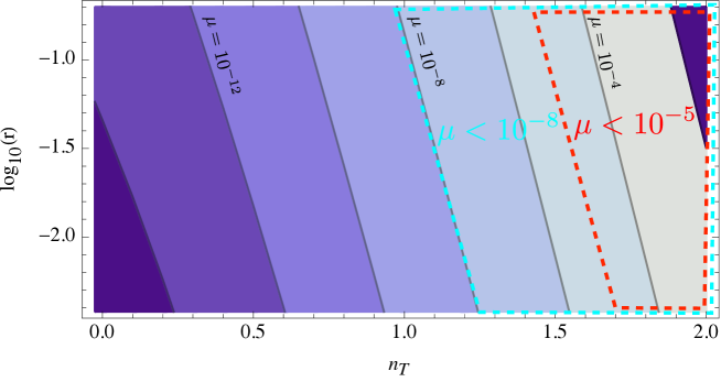
Figure 1: The magnitude of the chemical potential $\mu$ generated from primordial gravitational waves is shown in the $n_{T}$–$r$ plane. The regions enclosed by red dashed lines are ruled out by the COBE satellite. Those by cyan dashed ones can be probed by the PIXIE.

Note that this consequence is the result of the indirect energy transfer via CMB temperature fluctuations from gravitational waves. To understand this, let us discuss Eq. (3.19) again. For simplicity, we neglect the second terms, $ik\lambda F^{T}_{\gamma}$ and $\Lambda$, in both the center and the right-hand side, which describe the free streaming of the CMB photons and the anisotropic nature of Thomson scattering, respectively. Since the Thomson scattering time scale is much shorter than the cosmological time scale, we can take the steady state approximation between the center and the right hand side and obtain $2\partial_{\eta}h\sim-\dot{\tau}F^{T}_{\gamma}$. Accordingly we obtain

$$\dot{F}^{T}_{\gamma}\sim-\dot{\tau}F^{T}_{\gamma}\sim 2\partial_{\eta}h.$$ (4.1)

Eq. (4.1) tells us that the temperature fluctuations created by the integrated Sachs-Wolfe effect are decreasing during extremely short time interval by the Thomson scattering. Therefore, since the generated CMB distortion depends on how much CMB anisotropies are damped by the Thomson scattering, the contribution to the distortions is proportional to $F_{\gamma}\dot{F}_{\gamma}$.

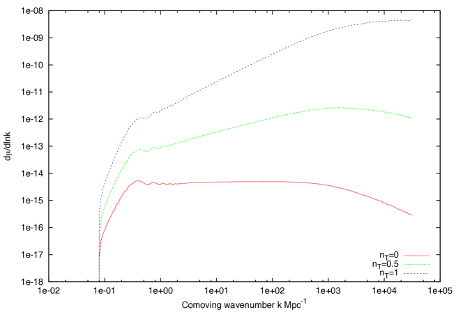
Figure 2: The amount of $\mu$ generated per the logarithmic $k$ interval originated from the tensor modes. The red, green, and blue lines correspond to the cases with $n_{T}=0$, $n_{T}=0.5$ and $n_{T}=1.0$, respectively.

4.2 Comparison with the scalar perturbation case

The CMB distortions originated from the scalar perturbations are mainly generated by the energy release due to Silk damping. In the similar way to Eq. (3.35), the chemical potential created from the scalar perturbations can be calculated from [21, 22]

$$\mu^{S}=1.4\cdot\frac{1}{4}\int^{\eta_{\rm fr}}_{0}d\eta^{\prime}\mathcal{J}_{DC}(\eta^{\prime})\int d(\ln k)\mathcal{P}_{\mathcal{R}}(k)$$

$$\dot{\tau} \bigg{[}-\frac{4}{3k^{2}}(\Theta_{e}-\Theta_{\gamma})^{2}-\sigma_{\gamma}(-18\sigma_{\gamma}+G^{S}_{\gamma 2}+G^{S}_{\gamma 0})+\sum_{l=3}(-1)^{n}(2n+1)F^{S}_{\gamma l}F^{S}_{\gamma l}\bigg{]},$$ (4.2)

where $F^{S}_{\gamma l}$ and $G^{S}_{\gamma l}$ are the Legendre-expansion coefficients for the scalar components of $F_{\gamma}$ and $G_{\gamma}$ defined in Eqs. (3.13) and (3.14). $\Theta_{\gamma}$, $\Theta_{e}$, and $\sigma_{\gamma}$ correspond to the photon fluid velocity, the baryon fluid velocity and the anisotropic stress of the photon fluid [27], which are explicitly written as

$$\Theta_{\gamma}=\frac{3}{4}kF^{S}_{\gamma 1},\quad\Theta_{e}=ikv,\quad\sigma_{\gamma}=\frac{1}{2}F^{S}_{\gamma 2},$$ (4.3)

with $v$ being the baryon fluid velocity potential.

For the case with the scalar mode, since the dominant generation mechanism is Silk damping, the $\mu$ distortion is generated around Silk damping scale (see Fig. 4 in Ref. [24]). On larger scales than Silk damping one, photon and baryon are tightly coupled before the epoch of recombination. In the tight coupling approximation, the velocity difference, $\Theta_{e}-\Theta_{\gamma}$ and the anisotropic stress $\sigma_{\gamma}$ is of the order of $k/\dot{\tau}\ll 1$. Therefore, the contributions from such large scales are negligible.

On the other hand, since the temperature fluctuations due to the tensor modes do not couple with the baryon fluids, they are not suppressed by the order of $k/\dot{\tau}$. As mentioned above, the temperature fluctuations can be approximated to $F^{T}_{\gamma}\sim-2\partial_{\eta}h/\dot{\tau}$ over all scales. Therefore, the generation of the chemical potential due to the tensor modes occurs even on larger scales, compared with Silk damping case.

Fig. 2 shows that scale dependence of $\mu$ distortion. In the figure, the vertical axis represents ${d\mu}/{d\ln k}$. Compared to the scalar mode cases (e.g. Fig. 4 in Ref. [24]), the $\mu$ distortion generated from the tensor mode comes even from larger scales. In particular, as one can see from Fig. 2, the contribution to the chemical potential dramatically increases around $k={\cal O}(0.1)$ Mpc^-1, which corresponds to the Horizon scale at the epoch $\eta_{\rm fr}$. This is because, after horizon crossing, the gravitational waves start to decay and produce the temperature fluctuations through the integrated Sachs-Wolfe effect. Fig. 2 also shows the cases for other values of $n_{T}$. As expected, the contribution from small scales increases for larger $n_{T}$.

5 Conclusions and discussion

In this paper, we have investigated CMB $\mu$ distortion originated from primordial gravitational waves. The temperature anisotropies generated from those are damped through the Thomson scattering, even on scales larger than Silk damping scale, which leads to the generation of the non-zero chemical potential $\mu$. Unfortunately, given the tensor-to-scalar ratio of the order of unity and the scale invariance of primordial gravitational waves, the created chemical potential $\mu$ is as small as $10^{-13}$. However, once the blue spectral index for tensor perturbations is allowed, the significant $\mu$ distortion can be generated, which in turn strongly constrains the tensor-to-scalar ratio and the tensor spectral index.

This new mechanism is quite different from that generated from the scalar perturbations, in which Silk damping effects mainly damp the temperature anisotropies while the damping is ineffective in the tight coupling region. Thus, the chemical potential $\mu$ can be produced even on larger scales for the tensor perturbations while that from the scalar perturbation is created mainly below Silk damping scale. This kind of the scale dependence may enable us to discriminate whether $\mu$ distortion is created from the tensor or the scalar perturbations, even if the former is much smaller than the latter. This is because, if we consider the cross correlation between the temperature anisotropies and the (scale dependent) $\mu$ distortion, their correlated bispectra can be large for the tensor mode compared to the scalar one since the tensor mode is dominant on scales larger than Silk damping scale while that from the scalar mode is significantly suppressed on such larger scales. We will study this issue in the future work.

Appendix A Mixing of Blackbodies

A.1 Mixing blackbodies to a new blackbody

Here let us consider two blackbody spectra with different temperatures, $T+\delta T$ and $T-\delta T$, respectively and mix them. The total energy density of this system is given by

$$\rho_{\text{initial}}=\frac{\alpha}{2}[(T+\delta T)^{4}+(T-\delta T)^{4}]=\alpha T^{4}\left[1+\frac{3}{2}\left(\frac{\delta T}{T}\right)^{2}+\cdots\right]^{4}=\rho_{\text{final}},$$ (A.1)

which is conserved. Assuming that the mixed system relaxes into one blackbody spectrum, the final temperature of a new blackbody one is given by

$$T_{\text{final}}=T\left[1+\frac{3}{2}\left(\frac{\delta T}{T}\right)^{2}+\cdots\right].$$ (A.2)

In this case, we can easily confirm that the final number density changes from the initial number density,

$$n_{\text{initial}}=\beta T^{3}\left[1+3\left(\frac{\delta T}{T}\right)^{2}+\cdots\right]\to n_{\text{final}}=\beta T_{\text{final}}^{3}=\beta T^{3}\left[1+\frac{9}{2}\left(\frac{\delta T}{T}\right)^{2}+\cdots\right].$$ (A.3)

This result implies that, only when the number is not conserved, the new system can relax into one blackbody.

A.2 Mixing blackbodies under both of energy and number conservations

In this subsection, we mix two blackbodies by imposing not only the energy conservation but also the number conservation. In this setting, as shown in the previous subsection, the new mixed system cannot relax into a blackbody, instead, relax into the Bose-Einstein system with a non-zero chemical potential.

For such a Bose-Einstein distribution, the energy and the number densities with a non-zero chemical potential $\mu$ are estimated up to the first order of $\mu$ as

$$\rho =\alpha T_{\text{BE}}^{4}\left(1-\frac{90\zeta(3)}{\pi^{4}}\mu\right)$$ (A.4)

$$n =\beta T^{3}_{\text{BE}}\left(1-\frac{\pi^{2}}{6\zeta(3)}\mu\right),$$ (A.5)

where $T_{\text{BE}}$ is the temperature of this Bose-Einstein distribution. From the number and the energy conservations, $\mu$ and $T_{\text{BE}}$ are easily estimated as [21],

$$\mu =\frac{1}{\left(\frac{\pi^{2}}{9\zeta(3)}-\frac{45\zeta(3)}{\pi^{4}}\right)}\left(\frac{\delta T}{T}\right)^{2},$$ (A.6)

$$T_{\text{BE}} =T\left[1+\frac{\frac{\pi^{2}}{6\zeta(3)}-\frac{45\zeta(3)}{\pi^{4}}}{\frac{\pi^{2}}{9\zeta(3)}-\frac{45\zeta(3)}{\pi^{4}}}\left(\frac{\delta T}{T}\right)^{2}\right].$$ (A.7)

It is now manifest that both of the temperature shift and the generated chemical potential are of the second order in $\delta T/T$.

References

- [1] G. Hinshaw et al. [WMAP Collaboration], arXiv:1212.5226 [astro-ph.CO].
- [2] P. A. R. Ade et al. [Planck Collaboration], arXiv:1303.5082 [astro-ph.CO].
- [3] A. A. Starobinsky, Phys. Lett. B 91, 99 (1980). A. H. Guth, Phys. Rev. D 23, 347 (1981); K. Sato, Mon. Not. Roy. Astron. Soc. 195, 467 (1981).
- [4] P. A. R. Ade et al. [BICEP2 Collaboration], arXiv:1403.3985 [astro-ph.CO].
- [5] Y. B. Zeldovich and R. A. Sunyaev, Astrophys. Space Sci. 4, 301 (1969).
- [6] R. A. Sunyaev and Y. B. Zeldovich Astrophys. Space Sci. 7, 20 (1970).
- [7] Danese, L.; de Zotti, G. : Double Compton process and the spectrum of the microwave background,Astronomy and Astrophysics, vol. 107, no. 1, Mar. 1982, p. 39-42. Research supported by the Consiglio Nazionale delle Ricerche.
- [8] C. Burigana, L. Danese, and G. de Zotti, Astron. Astrophysics, 246, 49 (1991)
- [9] W. Hu, D. Scott and J. Silk, Astrophys. J. 430, L5 (1994) [astro-ph/9402045].
- [10] J. Chluba, S. Y. .Sazonov and R. A. Sunyaev, [astro-ph/0611172].
- [11] R. Khatri and R. A. Sunyaev, JCAP 1206, 038 (2012) [arXiv:1203.2601 [astro-ph.CO]].
- [12] J. C. Mather, E. S. Cheng, D. A. Cottingham, R. E. Eplee, D. J. Fixsen, T. Hewagama, R. B. Isaacman and K. A. Jesnsen et al., Astrophys. J. 420, 439 (1994).
- [13] D. J. Fixsen, E. S. Cheng, J. M. Gales, J. C. Mather, R. A. Shafer and E. L. Wright, Astrophys. J. 473, 576 (1996) [astro-ph/9605054].
- [14] A. Kogut, D. J. Fixsen, D. T. Chuss, J. Dotson, E. Dwek, M. Halpern, G. F. Hinshaw and S. M. Meyer et al., JCAP 1107, 025 (2011) [arXiv:1105.2044 [astro-ph.CO]].
- [15] P. Andre et al. [PRISM Collaboration], arXiv:1306.2259 [astro-ph.CO].
- [16] R. A. Sunyaev and Y. .B. Zeldovich, Astrophys. Space Sci. 9, 368 (1970).
- [17] J. D. Barrow & P. Coles, Mon. Not. Roy. Astron. Soc., 248, 52 (1991).
- [18] R. A. Daly, Astrophys. J. 371, 14 (1991).
- [19] J. Silk, Astrophys. J. 151, 459 (1968).
- [20] J. Chluba and R. A. Sunyaev, Astron. Astrophys. 424, 389 (2003) [astro-ph/0404067].
- [21] R. Khatri, R. A. Sunyaev and J. Chluba, Astron. Astrophys. 543, A136 (2012) [arXiv:1205.2871 [astro-ph.CO]].
- [22] J. Chluba, R. Khatri and R. A. Sunyaev, Mon. Not. Roy. Astron. Soc. 425, 1129 (2012) [arXiv:1202.0057 [astro-ph.CO]].
- [23] J. Chluba and D. Grin, Mon. Not. Roy. Astron. Soc. 434, 1619 (2013) [arXiv:1304.4596 [astro-ph.CO]].
- [24] J. B. Dent, D. A. Easson and H. Tashiro, Phys. Rev. D 86, 023514 (2012) [arXiv:1202.6066 [astro-ph.CO]].
- [25] W. Hu and J. Silk, Phys. Rev. D 48, 485 (1993).
- [26] A. Kosowsky, Annals Phys. 246, 49 (1996) [astro-ph/9501045].
- [27] C. -P. Ma and E. Bertschinger, Astrophys. J. 455, 7 (1995) [astro-ph/9506072].
- [28] J. R. Bond and G. Efstathiou, Astrophys. J. 285, L45 (1984).
- [29] J. Lesgourgues, arXiv:1104.2932 [astro-ph.IM].
- [30] D. Blas, J. Lesgourgues and T. Tram, JCAP 1107, 034 (2011) [arXiv:1104.2933 [astro-ph.CO]].
- [31] J. Lesgourgues, arXiv:1104.2934 [astro-ph.CO].
- [32] J. Lesgourgues and T. Tram, JCAP 1109, 032 (2011) [arXiv:1104.2935 [astro-ph.CO]].
- [33] M. Gerbino, A. Marchini, L. Pagano, L. Salvati, E. Di Valentino and A. Melchiorri, arXiv:1403.5732 [astro-ph.CO].
- [34] Y. Wang and W. Xue, arXiv:1403.5817 [astro-ph.CO].
- [35] F. Wu, Y. Li, Y. Lu and X. Chen, arXiv:1403.6462 [astro-ph.CO].