Strongly reinforced Pólya urns with graph-based competition

Abstract

We introduce a class of reinforcement models where, at each time step $t$, one first chooses a random subset $A_{t}$ of colours (independent of the past) from $n$ colours of balls, and then chooses a colour $i$ from this subset with probability proportional to the number of balls of colour $i$ in the urn raised to the power $\alpha>1$. We consider stability of equilibria for such models and establish the existence of phase transitions in a number of examples, including when the colours are the edges of a graph, a context which is a toy model for the formation and reinforcement of neural connections.

Keywords: reinforcement model, Pólya urn, stochastic approximation algorithm, stable equilibria 2010 Mathematics Subject Classification : Primary: 60K35. Secondary: 37C10.

1 Introduction

Random processes with reinforcement have been studied mathematically since at least the early 1900s, and have connections to applied problems such as the design of clinical trials, and the formation of networks such as neural networks, the Internet, and social networks. One of the most simple and elegant of these models is known as Pólya’s urn: starting with one black and one red ball in an urn, select a ball at random from the urn, replace it, and add another of the same colour. The proportion $X_{t}$ of black balls in the urn after $t$ balls have been added is a bounded Martingale, and has a discrete uniform distribution for each $t$, whence there is a random variable $X\sim U[0,1]$ such that $\mathbb{P}(X_{t}\rightarrow X)=1$. Various generalisations of this model have been studied in the last hundred years or so, see e.g. [17, 22]. In recent times, reinforced random walks and preferential attachment models continue to be studied extensively.

One direction of generalisation of Pólya’s urn is to modify this selection probability (the probability of selecting a ball of a given colour). Fix $W:\mathbb{N}\rightarrow(0,\infty)$, and if $N_{t}^{\scriptscriptstyle(i)}$ is the number of balls of colour $i$ in the urn at time $t$, then at time $t+$ we select a ball of colour $i$ from the urn with probability $W(N_{t}^{\scriptscriptstyle(i)})/\sum_{j}W(N_{t}^{\scriptscriptstyle(j)})$. In Pólya’s urn, there are two colours and $W(x)=x$. A beautiful construction due to Rubin [8] shows that if $\sum_{x=1}^{\infty}W(x)^{-1}<\infty$ (sometimes called the strong reinforcement regime) then only one colour is chosen infinitely often. Otherwise each colour is chosen infinitely often, and if $W$ grows sufficiently slowly (e.g. $W(x)=x^{\alpha}$ for some $\alpha\in(0,1)$) then the proportions of each colour are equal in the limit.

A further direction of generalisation involves having multiple interacting urns, where colours may be present in more than one urn and where multiple balls may be added to one or more urns depending on what colour is selected. See for example the PhD Thesis (and related papers) of Launay [12, 13, 14], and recent work of Launay and Limic [15], and Benaim and coauthors [4, 3]. In such settings colours may not be competing with each other on every iteration of the process, and Rubin’s construction need not apply.

1.1 Our models

Consider the following simplistic model for the reinforcement of neural connections in the brain: A signal enters the brain at some (randomly) chosen neuron and is transmitted to a (random) single neighbouring neuron with probability depending on the relative efficiency of the synapses connecting the neurons, and in doing so the efficiency of the utilized synapse is improved/reinforced. We are interested in the structures and relative efficiency of neural networks that can arise from repeating this process a very large number of times, in a strong reinforcement regime.

With this motivation, we consider a large class of “interacting urn”-type models that we have not found in the literature. Suppose that we have $n$ colours of balls. Let $N_{t}^{\scriptscriptstyle(i)}$ be the number of balls of colour $i$ in our “urn” at time $t\in\mathbb{Z}_{+}$, and assume that $N_{0}^{\scriptscriptstyle(i)}=1$ for each $i\in[n]=\{1,2,\dots,n\}$. The process $\vec{N}_{t}=(N_{t}^{\scriptscriptstyle(i)}:i\in[n])$ evolves as follows. At time $t\in\mathbb{N}$ we choose a subset $A_{t}\subset[n]$ independently of $\mathcal{F}_{t-1}=\sigma\{A_{s},(N_{s}^{\scriptscriptstyle(i)}:i\in[n])\}_{0\leq s\leq t-1}$, according to some law. We then select a colour $i$ from the balls of colours in $A_{t}$ according to their current weights in the urn, i.e., given $A_{t}$, we select a ball of colour $i\in A_{t}$ with probability

$$\frac{W(N_{t-1}^{\scriptscriptstyle(i)})}{\sum_{j\in A_{t}}W(N_{t-1}^{\scriptscriptstyle(j)})}$$ (1)

then we replace that ball and add another of the same colour, so that $N_{t}^{\scriptscriptstyle(j)}=N_{t-1}^{\scriptscriptstyle(j)}+\mathds{1}_{\{j=i\}}$. For a fixed $n$, the law of such a model is then completely specified by the function $W$ and the law of $A_{1}$, so we will refer to any such model as a $(W,A)$-Reinforcement Model, or simply a WARM.

In [10] we consider the case $W(x)={\mathrm{e}}^{\gamma x}$ for some fixed $\gamma>0$. In this paper our results will be for reinforcement functions $W:\mathbb{N}\rightarrow(0,\infty)$ of the following kind:

Condition $(\alpha)$: $W(x)=x^{\alpha}$ for some fixed $\alpha>1$.

We will also assume the following condition.

Condition 1.1 (Subset selection).

The subsets $(A_{t})_{t\geq 0}$ are i.i.d. with $p_{\varnothing}=0$, where $p_{A}\equiv\mathbb{P}(A_{t}=A)$.

We are interested in the random vectors $\vec{X}_{t}=\vec{N}_{t}/(t+n)$ of proportions of balls of each colour, and more precisely their limits as $t\rightarrow\infty$. Any model with $p_{\varnothing}\in(0,1)$ can be considered as a random time change of a model with $p_{\varnothing}=0$, which does not affect the possible limits of $\vec{X}_{t}$. Thus we lose nothing in assuming that $p_{\varnothing}=0$ in Condition 1.1. For models with plenty of symmetry in terms of the colour labellings, we may instead consider the ordered vector $[\vec{X}_{t}]$, having the same elements as $\vec{X}_{t}$, but listed in decreasing order. Most of our examples satisfy the following symmetry property, which implies that $\mathbb{P}(|A_{1}|=m)=nm^{-1}a_{m}p_{m}$:

Condition 1.2 (Symmetry).

There exist $(p_{\ell})_{\ell=1}^{n}$ and $(a_{\ell})_{\ell=1}^{n}$ such that for every $m\geq 0$,

• $p_{A}\in\{0,p_{m}\}$ whenever $|A|=m$, and

• $\#\{A\ni i:|A|=m,p_{A}=p_{m}\}=a_{m}$ for every $i\in[n]$.

Condition 1.2 is somewhat unpalatable, so let us point out that many of the models considered in this paper satisfy the following stronger symmetry property, which implies that $\mathbb{P}(|A_{1}|=m)={n\choose m}p_{m}$, and also that (almost surely) at least $n-\underline{m}+1$ colours are chosen a positive proportion of the time, where $\underline{m}=\min\{m\geq 1:p_{m}>0\}$.

Condition 1.3 (Strong symmetry).

There exist $(p_{i})_{i=1}^{n}$ such that $p_{A}=p_{m}$ whenever $|A|=m$.

We are primarily interested in the setting where the colours $[n]$ are the edges (synapses) of a connected graph $G$ (brain) with $n_{v}$ vertices (neurons). In this setting we will assume the following.

Condition 1.4.

$V_{t}$ is chosen uniformly at random from the vertices of $G$, and $A_{t}$ is the set of edges incident to $V_{t}$.

WARMs where the law of $A_{1}$ corresponds to Condition 1.4 on some graph $G$ will be called WARM graphs. When $G$ is specified the WARM will be called a WARM (on) $G$.

1.2 Examples

We begin with two WARMs that are in general not WARM graphs.

Example 1.5 (Uniform, fixed $m$).

Fix $m\in[n]$ (the model becomes relatively trivial when $m=1$ or $m=n$) and choose $A_{t}$ with $|A_{t}|=m$ uniformly at random from $[n]$. Then $|A_{t}|=m$ almost surely and $\mathbb{P}(A_{t}=A)=m!(n-m)!/n!$ when $|A|=m$. This is the special case of Condition 1.3 with $p_{r}=0$ for all $r\neq m$. At least $n-m+1$ colours are each chosen a positive proportion of the time.

Example 1.6 (Bernoulli$(p)$).

Fix $p\in(0,1)$, and independently choose each colour to be in $A_{t}$ with probability $p$. After a parameter change (due to $p_{\varnothing}=(1-p)^{n}>0$), this is the special case of Condition 1.3 with $p_{m}=p^{m}(1-p)^{n-m}(1-p_{\varnothing})^{-1}$ for all $m\geq 1$. All $n$ colours are chosen a positive proportion of the time.

A natural extension of Example 1.6 would be to have a different $p$ for each colour. Turning to WARM graphs (i.e., assuming Condition 1.4 hereafter), observe that the special case of Example 1.6 with $n=2$ and $p=1/2$ is the same as the WARM on the star-graph on 2 edges.

Example 1.7 (WARM Star graph).

Let $G$ be the star-graph on $n_{v}=n+1$ vertices consisting of a central vertex connected by $n$ edges to $n$ leaves (vertices of degree 1). Then the WARM on $G$ is the special case of Condition 1.3 with $p_{1}=p_{n}=1/(n+1)$ and $p_{m}=0$ otherwise.

In the next two examples, $G$ is regular with degree $d=d(n)$ (so $|A_{t}|=d$ almost surely), so the WARM on $G$ satisfies Condition 1.2 with $p_{A}=0$ if $|A|\neq d$, and with $p_{d}=1/n_{v}$ and $a_{d}=2$ since any one of the $n_{v}$ vertices is equally likely to be $V_{t}$ and every edge is incident to 2 vertices. On the other hand there exist subsets of size $d$ that are chosen with probability 0 (so Condition 1.3 is not satisfied).

Example 1.8 (WARM Cycle graph).

Let $G$ be the cycle graph with $n$ edges and $n$ vertices. Each vertex is of degree $d=2$.

Example 1.9 (WARM Complete graph).

Let $G$ be the complete graph on $n_{v}$ vertices, with $n=n_{v}(n_{v}-1)/2$ edges. Each vertex is of degree $d=n_{v}-1$.

Note that Examples 1.9, 1.8, and 1.5 (with $m=2$) are all identical when $n=3$, and correspond to the WARM triangle graph which is studied extensively in Section 3.3. All of the above examples satisfy the symmetry property Condition 1.2. Let us now give a simple example that does not satisfy Condition 1.2(ii).

Example 1.10 (WARM Line/Path graph).

Let $G$ be the line segment with $n$ edges (and $n+1$ vertices). The two leaves have degree 1, while all interior vertices have degree 2.

Star graphs and the line graph with $n=3$ are special cases of whisker graphs (which also fails to satisfy Condition 1.2 in general) defined as follows.

Example 1.11 (WARM Whisker graph).

A whisker graph is defined as a tree with a diameter less than or equal to three. If the diameter is equal to two, then we obtain a star graph. If the diameter is equal to three, then we have a graph consisting of a distinguished edge $e$ with $r\geq 1$ leaves incident to one endvertex of $e$ and $s=n-(r+1)\geq 1$ leaves incident to the other endvertex (i.e. $G$ is constructed by connecting two star graphs by a single edge, $e$).

We believe that whisker graphs play a central role in the graph setting (see Conjecture 1.24).

1.3 Linearly stable equilibria

For fixed $n$ and $\vec{v}\in\Delta_{n}\equiv\{\vec{u}\in\mathbb{R}^{n}:u_{i}\geq 0,\sum_{i=1}^{n}u_{i}=1\}$, let $F\colon\Delta_{n}\rightarrow\mathbb{R}^{n}$ be defined (for a given WARM) by

$$F(\vec{v})_{i}=-v_{i}+\lim_{t\rightarrow\infty}\sum_{A\ni i}p_{A}\frac{W(v_{i}t)}{\sum_{j\in A}W(v_{j}t)}.$$ (2)

Definition 1.12 (Equilibrium).

For fixed $n$, a vector $\vec{v}\in\Delta_{n}$ is an equilibrium distribution for the WARM if $F(\vec{v})=\vec{0}$. We let $\mathcal{E}$ denote the set of equilibria for a given WARM, and write $\mathcal{E}_{\alpha}=\mathcal{E}$ when Condition $(\alpha)$ holds.

Intuitively this says that in the limit as $t\rightarrow\infty$, the proportion of balls of colour $i$ in the urn is equal to the probability that the next selected ball is of colour $i$. To see that the term inside the limit in (2) sums to 1, observe that

$$\sum_{i=1}^{n}\sum_{A\ni i}p_{A}\frac{W(v_{i}t)}{\sum_{j\in A}W(v_{j}t)}=\sum_{A\neq\varnothing}\sum_{i\in A}p_{A}\frac{W(v_{i}t)}{\sum_{j\in A}W(v_{j}t)}=\sum_{A\neq\varnothing}p_{A}=1.$$

Note that when $W(x)=x^{\alpha}$, $F(\vec{v})=\vec{0}$ reduces to

$$v_{i}= \sum_{A\ni i}p_{A}\cdot\frac{v_{i}^{\alpha}}{\sum_{j\in A}v_{j}^{\alpha}}.$$ (3)

Let the partial derivatives of $F$ at $\vec{v}$ be denoted by $D_{i,k}=\partial F(\vec{v})_{i}/\partial v_{k}$, whenever these quantities exist, and let ${\bf D}(\vec{v})$ denote the matrix with $(i,k)$ entry $D_{i,k}$ evaluated at the point $\vec{v}$.

Definition 1.13 (Stable equilibrium).

An equilibrium distribution $\vec{v}$ (i.e. satisfying (3)) is a linearly-stable equilibrium if all eigenvalues of ${\bf D}(\vec{v})$ have negative real parts, linearly-unstable equilibrium if some eigenvalue of ${\bf D}(\vec{v})$ has positive real part, and critical otherwise. Let $\mathcal{S}$ denote the set of linearly-stable equilibria for a given WARM, and write $\mathcal{S}_{\alpha}=\mathcal{S}$ when Condition $(\alpha)$ holds.

For a given WARM, let $\mathcal{A}$(=$\mathcal{A}_{\alpha}$ when Condition $(\alpha)$ holds) denote the (random, nonempty) set of accumulation points of the sequence $\vec{X}_{t}$. The main reason that we are interested in linearly-stable equilibria is because of the following theorem (and conjecture) whose proof (see Appendix A) relies on Theorem 1.16 below together with the general theory of the dynamical system approach to studying stochastic approximation algorithms, established by Benaïm and coauthors. See for example [4, Proposition 3.5, Theorem 3.9, Theorem 3.11].

Theorem 1.14 (Accumulation structure).

Assume Conditions $(\alpha)$ and 1.1. Then

1. almost surely $\mathcal{A}_{\alpha}\subset\mathcal{E}_{\alpha}$ and $\mathcal{A}_{\alpha}$ is a connected subset of $\Delta_{n}$,

2. $\mathbb{P}(\vec{X}_{t}\rightarrow\vec{v})>0$ for every $\vec{v}\in\mathcal{S}_{\alpha}$.

It follows from Theorem 1.14(i) that if $|\mathcal{E}_{\alpha}|<\infty$ then ($|\mathcal{A}_{\alpha}|=1$ almost surely so) $\vec{X}_{t}$ converges almost surely. Moreover, if $|\mathcal{E}_{\alpha}|=1$ then $\vec{X}_{t}$ converges almost surely to this unique equilibrium. We shall see that when $n=2$ and $\alpha=3$ in Example 1.7 there is a unique equilibrium ($\mathcal{E}_{\alpha}=\{(1/2,1/2)\}$, whence $\vec{X}_{t}$ almost surely converges to $(1/2,1/2)$) that is not linearly stable ($\mathcal{S}_{\alpha}=\varnothing$).

Conjecture 1.15 (Convergence to equlibirum).

For any WARM with $\alpha>1$, there exists a random vector $\vec{X}=(X_{1},\dots,X_{n})$, supported on the set of linearly-stable and critical equilibria such that $\mathbb{P}(\vec{X}_{t}\rightarrow\vec{X})=1$.

1.4 Main results

Our main results describe the set $\mathcal{S}_{\alpha}$ of linearly-stable equilibria in various situations, and hence (assuming Conjecture 1.15) the possible limiting proportions of balls of each colour. In particular we are interested in phase transitions in the set $\mathcal{S}_{\alpha}$ (including whether each colour can be chosen equally often) as $\alpha>1$ varies. Our first main result states that the number of linearly-stable equilibria is finite under Conditions $(\alpha)$ and 1.1.

Theorem 1.16 (Finite number of stable equilibria).

Assume Conditions ($\alpha$) and 1.1. Then $\mathcal{S}_{\alpha}$ is finite.

We will see some examples where $\mathcal{S}_{\alpha}=\varnothing$, but in many cases the existence of at least one linearly-stable equilibrium is given by the following results, when $\alpha>1$ is sufficiently small.

Lemma 1.17 ($\vec{1}/n$ equilibrium).

Assume Conditions 1.1 and 1.2. Then $\vec{1}/n\in\mathcal{E}_{\alpha}$.

Note that $\vec{1}/n$ is not an equilibrium for Example 1.10, which does not satisfy Condition 1.2. The eigenvalues associated to $\vec{1}/n\in\mathcal{E}_{\alpha}$ will be continuous functions of $\alpha$, giving rise to the transitions between the linear-stable and critical regions:

Proposition 1.18 (Stability of $\vec{1}/n$).

Assume Conditions 1.1, 1.3, $(\alpha)$, and that $p_{n}<1$. Then $\vec{1}/n\in\mathcal{S}_{\alpha}$ if and only if

$$\alpha<\frac{1}{n^{2}\sum_{m=2}^{n}\frac{p_{m}}{m^{2}}{n-2\choose m-2}}.$$ (4)

Moreover, $\vec{1}/n$ is critical if and only if equality holds in (4).

Here the right hand side is strictly larger than 1 when $p_{n}<1$, so under the assumptions of Proposition 1.18, $\vec{1}/n\in\mathcal{S}_{\alpha}$ for $\alpha>1$ but sufficiently close (depending on the model) to $1$, and $\vec{1}/n\notin\mathcal{S}_{\alpha}$ for $\alpha$ sufficiently large. In other words, all such models exhibit at least one phase transition. By applying Proposition 1.18 to various special cases one obtains the following:

Corollary 1.19 (Stability of $\vec{1}/n$ in Examples 1.5–1.7).

The equilibrium $\vec{1}/n$ is linearly-stable (critical when equality holds below) for:

• Example 1.5 if and only if

  $$\alpha<\frac{m(n-1)}{n(m-1)};$$

• Example 1.6 if and only if

  $$\alpha<\frac{1-(1-p)^{n}}{\sum_{m=2}^{n}p^{m}(1-p)^{n-m}\frac{n^{2}}{m^{2}}{n-2\choose m-2}};$$

• Example 1.7 if and only if $\alpha<n+1$.

The remaining examples have rather different behaviour:

Proposition 1.20 (Stability of $\vec{1}/n$ in Examples 1.8–1.9).

The equilibrium $\vec{1}/n$ is linearly-stable (critical when equality holds below) for:

• Example 1.8 if and only if $n$ is odd and $\alpha<\cos\left(\tfrac{\pi}{2n}\right)^{-2}$;

• Example 1.9 if and only if $n=3$ and $\alpha<4/3$.

Note that in the graph setting, when $\vec{v}=\vec{1}/n$, the matrix of partial derivatives is related to the edge-adjacency matrix. Typically $\vec{1}/n$ is not the only equilibrium, and indeed we will see many more examples of linearly-stable equilibria for various models. See for example Corollary 3.1 in the case of Example 1.5. If Condition 1.4 (and Condition 1.1) is satisfied then by the law of large numbers, any $\vec{v}\in\mathcal{E}$ must satisfy $v_{i}\leq 2/n_{v}$ for each edge $i$, since each edge is incident to 2 vertices. Similarly, for any $i$ incident to a leaf we have $v_{i}\geq 1/n_{v}$.

The following result often allows one to find stable equilibria in large systems by finding stable equilibria in smaller systems.

Lemma 1.21 (Stability reduction).

Suppose that $p_{A}=\mathbb{P}(A_{t}=A)$ for each $A\subset[n]$, with $p_{\{n\}}=0$, and define $p^{\prime}_{A\setminus\{n\}}=p_{A}$. Then $\vec{v}=(v_{1},\dots,v_{n-1},0)$ is a (linearly-stable) equilibrium for the WARM $(p_{A})_{A\subset[n]}$ if and only if $\vec{v}^{\prime}=(v_{1},\dots,v_{n-1})$ is a (linearly-stable) equilibrium for the WARM $(p^{\prime}_{A^{\prime}})_{A^{\prime}\subset{\bf C}_{n-1}}$.

The most important consequence of Lemma 1.21 for us is in the graph setting. Let $G$ be a graph with vertex set $V$ and edge set $E$, and let $n_{v}=|V|$. Let $G_{1},\dots,G_{k}$ be connected subgraphs of $G$ with $E_{j}=\{e_{1},\dots,e_{|E_{j}|}\}$ and $V_{j}$ denoting the edge set and vertex set respectively of $G_{j}$. Let

$$\mathcal{G}_{\scriptscriptstyle G}=\big{\{}{\bf G}=\{G_{j}\}_{j=1}^{k}:k\leq n_{v}/2,\,|V_{j}|\geq 2\text{ for each }j,\,V=\cup_{j=1}^{k}V_{j},\,V_{j}\cap V_{j^{\prime}}=\varnothing\text{ for all }j\neq j^{\prime}\big{\}},$$ (5)

denote the $V$-spanning collections of non-trivial connected clusters of $G$, and let ${\bf E}=\cup_{j=1}^{k}E_{j}$. Let $\mathcal{E}_{\scriptscriptstyle G}$ and $\mathcal{S}_{\scriptscriptstyle G}$ denote the equilibria and linearly stable equilibria for a WARM on $G$.

Theorem 1.22 (Subgraph stability reduction).

Fix $G$, and let

$${\bf G}=\{G_{j}\}_{j=1}^{k}\in\mathcal{G}_{\scriptscriptstyle G}\qquad\text{and}\qquad\vec{v}=\big{(}(v_{e})_{e\in E_{1}},(v_{e})_{e\in E_{2}},\dots,(v_{e})_{e\in E_{k}},(0)_{e\in E\setminus{\bf E}}\big{)}.$$

Then, for any WARM on $G$,

• $\vec{v}\in\mathcal{E}_{\scriptscriptstyle G}$ if and only if $\frac{|V|}{|V_{j}|}(v_{e})_{e\in E_{j}}\in\mathcal{E}_{\scriptscriptstyle G_{j}}$ for each $j=1,\dots,k$,

• $\vec{v}\in\mathcal{S}_{\scriptscriptstyle G}$ if and only if $\frac{|V|}{|V_{j}|}(v_{e})_{e\in E_{j}}\in\mathcal{S}_{\scriptscriptstyle G_{j}}$ for each $j=1,\dots,k$.

Definition 1.23 ($(G,\alpha)$-stable allocation).

Given a graph $G$, $\alpha>1$ and ${\bf G}\in\mathcal{G}_{\scriptscriptstyle G}$, we say that ${\bf G}$ admits a $(G,\alpha)$-stable allocation if there exists $\vec{v}$ with $v_{e^{\prime}}>0$ for all $e^{\prime}\in{\bf E}$ and $v_{e}=0$ for all $e\in E\setminus{\bf E}$ such that $\vec{v}\in(\mathcal{S}_{\alpha})_{\scriptscriptstyle G}$ or $\vec{v}$ is critical.

An element ${\bf G}$ of $\mathcal{G}_{\scriptscriptstyle G}$ is said to be a whisker-forest (resp. star-forest) if each component $G_{j}$ is a whisker (resp. star) graph.

Conjecture 1.24 (Whisker-forest conjecture).

Let $G$ be any graph. There exists $\alpha_{\scriptscriptstyle G}$ such that, for all $\alpha>\alpha_{\scriptscriptstyle G}$,

• any whisker-forest ${\bf G}$ on $G$ admits a $(G,\alpha)$-stable allocation;

• for any $\vec{v}\in(\mathcal{S}_{\alpha})_{\scriptscriptstyle G}$, there exists a whisker-forest ${\bf G}$ on $G$ such that: $v_{e}>0$ if and only if $e\in{\bf E}$.

As in Conjecture 1.24(ii), we believe that when $\alpha$ is large enough (depending on $G$), all stable equilibria live on whisker forests. What we have proved in this direction is the following result, which follows from an explicit characterisation (see Theorem 3.3) of $\mathcal{S}_{\alpha}$ for the WARM star graph:

Theorem 1.25 ($(G,\alpha)$-stable allocation for star-forests).

For any graph $G$, and $\alpha>1$, any star-forest ${\bf G}$ on $G$ admits a $(G,\alpha)$-stable allocation.

For large $\alpha$, this result can be extended to symmetric-whisker-forests, where each non-star component is symmetric (i.e. $s=r$) due to the following result:

Theorem 1.26 (Symmetric whisker graphs).

For every symmetric ($s=r$) whisker graph $G$, there exists $\alpha_{\scriptscriptstyle G}>1$ such that for all $\alpha>\alpha_{\scriptscriptstyle G}$, $(\mathcal{S}_{\alpha})_{\scriptscriptstyle G}$ is non-empty. Consequently, any symmetric whisker-forest ${\bf G}$ on $G$ admits a $(G,\alpha)$-stable allocation, if $\alpha$ is sufficiently large (depending on ${\bf G}$).

1.5 Overview of the paper

In Section 2 we prove Theorem 1.16, Lemma 1.17, Proposition 1.18, and Theorem 1.22. In Section 3 we obtain more detailed results on the existence of linearly-stable equilibria for various examples. In Section 4 we discuss some open problems, in particular some related to Conjecture 1.24. The proof of Theorem 1.14 follows the standard approach and is relegated to Appendix A.

2 Proofs of general results

In this section we prove the general results of Section 1.4, assuming Conditions 1.1 and $(\alpha)$ throughout. We opt for a proof of Theorem 1.22 instead of proving Lemma 1.21. We therefore begin this section with the proof that there are only finitely many stable equilibria.

2.1 Proof of Theorem 1.16

Fix $\alpha>1$. For $n=1$, the claim is trivial. The proof proceeds via induction over $n$, assuming that the result holds for all $n^{\prime}<n$.

Let $\vec{v}=(v_{1},\dots,v_{n})\in\mathcal{E}_{\alpha}$ denote an equilibrium distribution, so that

$$F(\vec{v})=\vec{0},$$ (6)

where

$$F_{i}(\vec{v})=-v_{i}+\sum_{A\ni i}p_{A}\frac{v_{i}^{\alpha}}{\sum_{k\in A}v_{k}^{\alpha}},\quad\qquad\text{ for }i\in[n].$$ (7)

We assume $v_{i}\neq 0$ for all $i\in[n]$. If an equilibrium is linearly stable for the system of $n$ equations and there is some $I\neq\varnothing$ such that $v_{i}=0$ for all $i\in I$, then it is linearly stable for the system on $[n]\setminus I$ (see Lemma 1.21 or [4, Corollary 3.8]).

Let $A\subset[n]$ be non-empty. Since $\alpha>1$, using Hölder’s inequality we have

$$\sum_{k\in A}v_{k}^{\alpha}\geq\biggl{(}\sum_{k\in A}v_{k}\biggr{)}^{\alpha}|A|^{1-\alpha}.$$ (8)

By the law of large numbers, the set $A$ is chosen a proportion $p_{A}$ of the time (in the limit as $t\rightarrow\infty$). It follows that colours contained in $A$ are chosen at least $p_{A}$ proportion of the time, hence

$$\sum_{k\in A}v_{k}\geq p_{A}.$$ (9)

Equations (8) and (9) yield

$$\sum_{k\in A}v_{k}^{\alpha}\geq p^{\alpha}_{A}|A|^{1-\alpha}.$$ (10)

Inserting this into (6) we obtain

$$v_{i}^{1-\alpha}=\sum_{A\ni i}p_{A}\frac{1}{\sum_{k\in A}v_{k}^{\alpha}}\leq\sum_{A\ni i}p_{A}p^{-\alpha}_{A}|A|^{\alpha-1}.$$

Thus,

$$v_{i}\geq\biggl{(}\sum_{A\ni i}(p_{A}/|A|)^{1-\alpha}\biggr{)}^{1/(1-\alpha)}.$$

This shows that there exists a (model dependent) $\varepsilon>0$ such that there is no $\vec{v}\in\mathcal{E}_{\alpha}$ satisfying $0<v_{i}<\varepsilon$ for some $i\in[n]$. It remains to prove that for any $\varepsilon>0$ there are only finitely many $\vec{v}\in\mathcal{S}_{\alpha}$ satisfying $v_{i}\geq\varepsilon$ for all $i\in[n]$.

Fix $\varepsilon>0$, and choose $\delta\in(0,\frac{\pi}{2\alpha})$ and define $H^{n}\subset\mathbb{C}^{n}$ to be the Cartesian product of $n$ copies of the open complex domain

$$H:=\biggl{\{}z\in\mathbb{C}:\frac{\varepsilon}{2}<|z|<2,|\arg(z)|<\delta\biggr{\}}.$$

Since, for $z\in H$,

$$|\arg(z^{\alpha})|=\alpha|\arg(z)|<\alpha\delta<\pi/2,$$

we see that $\textnormal{Re}(z^{\alpha})>0$ for all $z\in H$. Therefore for non-empty $A$, $\textnormal{Re}\big{[}\sum_{k\in A}v_{k}^{\alpha}\big{]}>0$ for $\vec{v}\in H^{n}$, in particular, all functions $\vec{v}\mapsto\sum\limits_{k\in A}v_{k}^{\alpha}$ are analytic and zero-free in $H^{n}$, which shows that the functions

$$\vec{v}\mapsto\frac{v_{i}^{\alpha}}{\sum\limits_{k\in A}v_{k}^{\alpha}}$$

are also analytic in $H^{n}$, so finally we conclude that the functions $F_{i}(\vec{v})$ are analytic in $H^{n}$.

Next, define the map $F\colon H^{n}\mapsto\mathbb{C}^{n}$ by $F(\vec{v})=(F_{1}(\vec{v}),F_{2}(\vec{v}),\dots,F_{n}(\vec{v}))$ and the set

$${\mathcal{H}}:=\{\vec{v}\in H^{n}\colon F(\vec{v})=\vec{0}\;{\textnormal{ and }}{\textnormal{det}}\left[{\bf D}(\vec{v})\right]\neq 0\}.$$

Clearly $\mathcal{S}_{\alpha}\subset{\mathcal{H}}$. Our goal is to show that (i) ${\mathcal{H}}$ is a set of isolated points and (ii) it does not have accumulation points in the interior of the domain $H^{n}$.

To prove (i), let $\vec{w}\in{\mathcal{H}}$. Since $F(\vec{w})=\vec{0}$ and ${\textnormal{det}}\left[{\bf D}(\vec{w})\right]\neq 0$, due to the Implicit Function Theorem (see [24, Theorem 2, page 40]) there exists a biholomorphic map between some neighborhoods $U\ni\vec{w}$ and $V\ni\vec{0}$ (that is, a bijective holomorphic function whose inverse is also holomorphic). Since the map is bijective, there are no other solutions to the system $F_{i}(\vec{v})=0$, $i\in[n]$ in $U$, which shows that each element of ${\mathcal{H}}$ must be an isolated point.

To prove (ii), let us assume the converse, i.e., there exists a point $\vec{w}\in H^{n}$ which is an accumulation point of ${\mathcal{H}}$. Define

$${\mathcal{Z}}:=\{\vec{v}\in H^{n}\colon F(\vec{v})=\vec{0}\},$$

so ${\mathcal{Z}}$ is an analytic set in the sense of [24, Definition 1, page 129], and clearly ${\mathcal{H}}\subseteq{\mathcal{Z}}$. According to [23, Theorem 2.2, page 52], there exists a neighborhood $\Delta\subset H^{n}$ of the point $\vec{w}$, such that the analytic set $\Delta\cap{\mathcal{Z}}$ can be decomposed into a finite number of pure-dimensional analytic sets. Pure-dimensional means that the set has the same dimension at each point. One of these pure-dimensional analytic sets must have dimension zero (since we have assumed that $\vec{w}$ is an accumulation point for isolated points in ${\mathcal{H}}$, and isolated points are zero-dimensional). It is also clear that this zero-dimensional analytic set must have an accumulation point at $\vec{w}$. Now we use [24, Theorem 6 on page 135], which says that this is impossible: any zero-dimensional analytic set in $\Delta$ cannot have limit points inside $\Delta$. Therefore, we have arrived at a contradiction.

So far we have proved that the set ${\mathcal{H}}$ consists of isolated points and does not have accumulation points in the interior of $H^{n}$. Since the set

$$B:=\{\vec{v}\in\mathbb{C}^{n}\colon\textnormal{Im}(v_{i})=0,\;\;\;\varepsilon\leq\textnormal{Re}(v_{i})\leq 1\}$$

is compact in $\mathbb{C}^{n}$, we conclude that the set $B\cap H^{n}$ is finite. Since stable equilibria are elements of $B\cap H^{n}$, this shows that we can have only finitely many $\vec{v}\in\mathcal{S}_{\alpha}$ satisfying $v_{i}>\varepsilon$ for each $i$. ∎

2.2 Proof of Lemma 1.17 and Proposition 1.18

Proof of Lemma 1.17. Assume that Condition 1.2 holds. Then, for $\vec{v}=\vec{1}/n$, the right hand side of (3) becomes

$$\sum_{A\ni i}\frac{p_{A}}{|A|}=\sum_{m=1}^{n}\sum_{\stackrel{{\scriptstyle A\ni i:}}{{|A|=m}}}\frac{p_{A}}{m}=\sum_{m=1}^{n}\frac{a_{m}p_{m}}{m},$$ (11)

which does not depend on $i\in[n]$. Since these quantities sum to 1, it follows that the right hand side of (3) is equal to $1/n$ for each $i$, which proves that $\vec{1}/n$ is an equilibrium (i.e., Lemma 1.17). ∎

Recall that the adjugate matrix $\mathrm{adj}{\bf A}$ of a square matrix ${\bf A}$ is given by $\mathrm{adj}{\bf A}={\bf C}^{\mathrm{T}}$, i.e., the transpose of the cofactor matrix ${\bf C}$ of ${\bf A}$. Recall that if ${\bf A}$ is a diagonal matrix with entries $A_{ii}$, then its cofactor matrix is a diagonal matrix ${\bf C}$ with $C_{ii}=\prod_{j\neq i}A_{jj}$, and its adjugate matrix is a diagonal matrix $\mathrm{adj}{\bf A}={\bf C}^{\mathrm{T}}={\bf C}$. In order to prove Proposition 1.18, we will use the following modification of the Matrix Determinant Lemma, which we have not found in the literature (although we expect that it is well known).

Lemma 2.1 (Modified Matrix Determinant Lemma).

If ${\bf R}\in\mathbb{R}^{n\times n}$ and $\vec{y},\vec{w}\in\mathbb{R}^{n}$ are column vectors then

$$\det({\bf R}+\vec{y}\vec{w}^{\mathrm{T}})=\det({\bf R})+\vec{w}^{\mathrm{T}}\mathrm{adj}({\bf R})\vec{y}.$$ (12)

Proof.

If ${\bf R}$ is invertible, then the matrix determinant lemma gives

$$\det({\bf R}+\vec{y}\vec{w}^{\mathrm{T}})=(1+\vec{w}^{\mathrm{T}}{\bf R}^{-1}\vec{y})\det({\bf R})=\det({\bf R})+\vec{w}^{\mathrm{T}}{\bf R}^{-1}\det({\bf R})\vec{y}=\det({\bf R})+\vec{w}^{\mathrm{T}}\mathrm{adj}({\bf R})\vec{y}.$$

If ${\bf R}$ is not invertible then ${\bf R}$ has some eigenvalues that are zero (and possibly some non-zero) and there exists some $\varepsilon_{0}$ (corresponding to the smallest magnitude-non-zero eigenvalue) such that no $\varepsilon\in(0,\varepsilon_{0})$ is an eigenvalue for ${\bf R}$, i.e., $\det({\bf R}-\varepsilon{\bf I})\neq 0$ for all such $\varepsilon$. Therefore, ${\bf R}-\varepsilon{\bf I}$ is invertible for any such $\varepsilon$. It follows that for all $\varepsilon\in(0,\varepsilon_{0})$

$$\det({\bf R}-\varepsilon{\bf I}+\vec{y}\vec{w}^{\mathrm{T}})=\det({\bf R}-\varepsilon{\bf I})+\vec{w}^{\mathrm{T}}\mathrm{adj}({\bf R}-\varepsilon{\bf I})\vec{y}.$$ (13)

We obtain the desired conclusion by taking the limit as $\varepsilon\downarrow 0$ on both sides of (13), and using the facts that all entries of $\mathrm{adj}({\bf R})$ are just sums and differences of minors (determinants of submatrices), and determinants are continuous functions of ${\bf R}$ (in the natural sense). ∎

Proof of Proposition 1.18. When $W(x)=x^{\alpha}$, (2) becomes

$$F(\vec{v})_{i}=-v_{i}+\sum_{A\ni i}p_{A}\frac{v_{i}^{\alpha}}{\sum_{j\in A}v_{j}^{\alpha}},$$

so that

$$D_{i,i}(\vec{v})=-1+\alpha v_{i}^{\alpha-1}\sum_{A\ni i}p_{A}\frac{\sum_{j\in A}v_{j}^{\alpha}-v_{i}^{\alpha}}{\left(\sum_{j\in A}v_{j}^{\alpha}\right)^{2}},$$ (14)

and, for $k\neq i$,

$$D_{i,k}(\vec{v})=-\alpha v_{k}^{\alpha-1}v_{i}^{\alpha}\sum_{A\ni i,k}p_{A}\frac{1}{\left(\sum_{j\in A}v_{j}^{\alpha}\right)^{2}}.$$ (15)

When $\vec{v}=\vec{1}/n$, this reduces to

$$D_{i,i}(\vec{1}/n)= -1+\alpha n\sum_{A\ni i}p_{A}\frac{|A|-1}{|A|^{2}},$$ (16)

$$D_{i,k}(\vec{1}/n)= -\alpha n\sum_{A\ni i,k}p_{A}\frac{1}{|A|^{2}}.$$ (17)

Assume that Condition 1.3 holds. Then, (16) can be written as

$$D_{i,i}(\vec{1}/n)= -1+\alpha n\sum_{m=1}^{n}p_{m}\sum_{A:|A|=m,i\in A}\frac{m-1}{m^{2}}$$

$$= -1+\alpha n\sum_{m=2}^{n}\frac{p_{m}}{m^{2}}{n-1\choose m-1}(m-1)$$

$$\equiv -1+\beta,$$ (18)

$$D_{i,k}(\vec{1}/n)= -\alpha n\sum_{m=2}^{n}\frac{p_{m}}{m^{2}}{n-2\choose m-2},\quad\text{ for }k\neq i$$

$$\equiv \delta<0.$$

To compute the eigenvalues of ${\bf D}(\vec{1}/n)$, observe that

$${\bf H}\equiv{\bf D}-\lambda{\bf I}=(-(1+\lambda)+\beta-\delta){\bf I}+\vec{1}(\delta\vec{1})^{\mathrm{T}}.$$

Hence, by Lemma 2.1, the determinant of ${\bf H}$ is

$$(-(1+\lambda)+\beta-\delta)^{n}+\sum_{i=1}^{n}\delta(-(1+\lambda)+\beta-\delta)^{n-1}.$$

This is equal to zero when

$$\lambda=\beta-\delta-1,\qquad\text{ or }\qquad\lambda=(n-1)\delta+\beta-1=-1.$$

The first eigenvalue satisfies

$$\lambda= \alpha n\sum_{m=2}^{n}\frac{p_{m}}{m^{2}}{n-1\choose m-1}(m-1)+\alpha n\sum_{m=2}^{n}\frac{p_{m}}{m^{2}}{n-2\choose m-2}-1$$

$$= \alpha n^{2}\sum_{m=2}^{n}\frac{p_{m}}{m^{2}}{n-2\choose m-2}-1,$$

which is continuous and increasing in $\alpha$, and is $<0$ if and only if

$$\alpha<\frac{1}{n^{2}\sum_{m=2}^{n}\frac{p_{m}}{m^{2}}{n-2\choose m-2}},$$

as required. ∎

2.3 Proof of Theorem 1.22

Under Condition 1.4, $p_{A}=1/|V|$ for every $A$ that is the set of edges incident to some vertex, and of course every edge $e$ is an edge in exactly two such $A$. For a vertex $x$ and an edge $e$ write $x\in e$ if $e=(x,x^{\prime})=(x^{\prime},x)$ for some $x^{\prime}\in V$ (i.e. if $x$ is an endvertex of $e$). Then the equilibrium equation for $e\notin{\bf E}$ is $0=0$, while for $e\in E_{j}$ it is

$$v_{e}= \sum_{A\ni e}p_{A}\frac{v_{\mathrm{e}}^{\alpha}}{\sum_{e^{\prime}\in A}v_{e^{\prime}}^{\alpha}}=\sum_{\stackrel{{\scriptstyle x\in V:}}{{x\in e}}}\frac{1}{|V|}\frac{v_{\mathrm{e}}^{\alpha}}{\sum_{\stackrel{{\scriptstyle e^{\prime}\in E:}}{{x\in e^{\prime}}}}v_{e^{\prime}}^{\alpha}}$$ (19)

$$= \sum_{\stackrel{{\scriptstyle x\in V_{j}:}}{{x\in e}}}\frac{1}{|V|}\frac{v_{\mathrm{e}}^{\alpha}}{\sum_{\stackrel{{\scriptstyle e^{\prime}\in E_{j}:}}{{x\in e^{\prime}}}}v_{e^{\prime}}^{\alpha}+\sum_{\stackrel{{\scriptstyle e^{\prime}\notin E_{j}:}}{{x\in e^{\prime}}}}v_{e^{\prime}}^{\alpha}},$$ (20)

where Let $e^{\prime}\notin E_{j}$ but $x\in e^{\prime}$ and $x\in V_{j}$. Then we have by definition of ${\bf G}$ that $x\notin V_{i}$ for $i\neq j$, so $e^{\prime}\notin E_{i}$ for any $i$. This means that $v_{e^{\prime}}=0$. It follows that the second sum in the denominator of (20) vanishes, so

$$v_{e}= \sum_{\stackrel{{\scriptstyle x\in V_{j}:}}{{x\in e}}}\frac{1}{|V|}\frac{v_{\mathrm{e}}^{\alpha}}{\sum_{\stackrel{{\scriptstyle e^{\prime}\in E_{j}:}}{{x\in e^{\prime}}}}v_{e^{\prime}}^{\alpha}},\quad\text{ and therefore }\quad\frac{|V|}{|V_{j}|}v_{e}=\sum_{\stackrel{{\scriptstyle x\in V_{j}:}}{{x\in e}}}\frac{1}{|V_{j}|}\frac{(\frac{|V|}{|V_{j}|}v_{e})^{\alpha}}{\sum_{\stackrel{{\scriptstyle e^{\prime}\in E_{j}:}}{{x\in e^{\prime}}}}(\frac{|V|}{|V_{j}|}v_{e^{\prime}})^{\alpha}},$$ (21)

which is (19) for the graph $G_{j}\ni e$ and appropriately rescaled $v$ components. This proves the first claim.

For the second claim, note that if $e\in E_{j}$ and $e^{\prime}\notin E_{j}$ then for $\vec{v}$ as in the theorem $F(\vec{v})_{e}$ does not depend on $v_{e}^{\prime}$. Thus for such $e,e^{\prime}$ we have $D_{e,e^{\prime}}=0$. It follows that ${\bf D}(\vec{v})$ is a block diagonal matrix of the form

$${\bf D}=\begin{pmatrix}{\bf D^{\scriptscriptstyle(1)}}&0&\cdots&0\\ 0&{\bf D^{\scriptscriptstyle(2)}}&\cdots&0\\ \vdots&\vdots&\ddots&\vdots\\ 0&0&\cdots&{\bf D^{\scriptscriptstyle(k+1)}}\end{pmatrix},$$

where ${\bf D^{\scriptscriptstyle(i)}}$ is the ${\bf D}$ matrix for $G_{i}$ for $i\leq k$ and where ${\bf D^{\scriptscriptstyle(k+1)}}=-{\bf I}_{|E\setminus{\bf E}|}$, and ${\bf I}_{m}$ denotes the identity matrix of dimension $m$. Thus the eigenvalues of ${\bf D}$ are simply those of each ${\bf D^{\scriptscriptstyle(i)}}$, $i\in[k+1]$ combined. Since the eigenvalue of ${\bf D^{\scriptscriptstyle(k+1)}}$ is $-1<0$, the result follows. ∎

3 Special cases

In this section, we examine some of our examples more carefully, beginning with one of the non-graphical WARMs.

3.1 Fixed $m$, uniform $A_{t}$ model

Recall that for this model, defined in Example 1.5, at least $n-m+1$ colours must be each chosen a positive proportion of the time. It is not too hard to prove that with positive probability $m-1$ of the colours are never chosen, from which it follows that with positive probability exactly $n-m+1$ colours are each chosen a positive proportion of the time.

From (3) $\vec{v}$ is an equilibrium if and only if

$$v_{i}= {n\choose m}^{-1}\sum_{\stackrel{{\scriptstyle A\ni i:}}{{|A|=m}}}\frac{v_{i}^{\alpha}}{\sum_{j\in A}v_{j}^{\alpha}}.$$ (22)

The first claim of Corollary 1.19 follows directly from Proposition 1.18 with $p_{m}={n\choose m}^{-1}$ for each of the ${n\choose m}$ subsets of size $m$. The following extension of this result could be obtained from Lemmas 1.21 and 1.17, and Proposition 1.18, by keeping track of the $p^{\prime}_{s}$ for various values of $s$ after $n-k$ colours have been removed. However, a direct proof is also not too hard, as we will see in the following.

Here and elsewhere, we use the notation $(u)_{k}$ to denote the vector $(u,\dots,u)\in\mathbb{R}^{k}$.

Corollary 3.1 (Stability in the fixed $m$, uniform $A_{t}$ model).

Let $k\geq n-m+1$. Then $\vec{v}=((1/k)_{k},(0)_{n-k})\in\mathcal{E}_{\alpha}$ for all $\alpha$, and $\vec{v}\in\mathcal{S}_{\alpha}$ if and only if

$$\alpha<\dfrac{\displaystyle{n\choose m}}{k^{2}\displaystyle{\sum_{r=(m-k)\vee 0}^{\scriptscriptstyle(n-k)\wedge(m-2)}{n-k\choose r}\frac{1}{(m-r)^{2}}{k-2\choose m-r-2}}},$$

while $\vec{v}$ is critical if equality holds.

Proof.

With $\vec{v}$ of the given form we have that (14)-(15) reduces to $D_{i,i}=-1$ and $D_{i,\ell}=D_{\ell,i}=0$ for $i>k$. For $i\leq k$, using the fact that $n-k\leq m-1$, and that $m-r-1=0$ if $r=m-1$ we have with $s^{\prime}=(n-k)\wedge(m-2)$,

$$D_{i,i}= -1+{n\choose m}^{-1}\alpha k\sum_{r=s}^{s^{\prime}}{k-1\choose m-r-1}{n-k\choose r}\frac{m-r-1}{(m-r)^{2}},$$

$$D_{i,\ell}= -{n\choose m}^{-1}\alpha k\sum_{r=s}^{s^{\prime}}{k-2\choose m-r-2}{n-k\choose r}\frac{1}{(m-r)^{2}}.$$

Using Lemma 2.1,

$$\det({\bf D}-\lambda{\bf I})=(-(1+\lambda))^{n-k})(a^{k}+ba^{k-1}k)=(-(1+\lambda))^{n-k}a^{k-1}(a+bk),$$

with

$$b= -{n\choose m}^{-1}\alpha k\sum_{r=s}^{s^{\prime}}{k-2\choose m-r-2}{n-k\choose r}\frac{1}{(m-r)^{2}}$$

$$a= -(1+\lambda)+{n\choose m}^{-1}\alpha k\sum_{r=s}^{s^{\prime}}{k-1\choose m-r-1}{n-k\choose r}\frac{m-r-1}{(m-r)^{2}}-b$$

$$= -(1+\lambda)+{n\choose m}^{-1}\alpha k^{2}\sum_{r=s}^{s^{\prime}}{n-k\choose r}\frac{1}{(m-r)^{2}}{k-2\choose m-r-2}.$$

The term $a+bk$ can be computed explicitly and equals $-(1+\lambda)$, i.e., $\lambda=-1$.

Note that $k-1\geq 1$ since $m<n$, so it remains to consider the case $a=0$, i.e.,

$$\lambda=-1+{n\choose m}^{-1}\alpha k^{2}\sum_{r=s}^{s^{\prime}}{n-k\choose r}\frac{1}{(m-r)^{2}}{k-2\choose m-r-2},$$

which is continuous and increasing in $\alpha$ and is negative if and only if

$$\alpha<\dfrac{{n\choose m}}{k^{2}\sum_{r=s}^{s^{\prime}}{n-k\choose r}\frac{1}{(m-r)^{2}}{k-2\choose m-r-2}}.$$

∎

3.2 Star graph

Throughout this section, we consider a WARM star graph on $n$ edges. First we describe the situation where $n=2$ (which is the same as the simplest line graph, and which also corresponds (after a time-change) to Example 1.6 with $n=2$ and $p=1/2$).

Theorem 3.2 (Equilibria and stability for star graph with two edges).

For the star graph with two edges the following is true: For $\alpha=3$, $\mathcal{E}_{\alpha}=\{(1/2,1/2)\}$ and this equilibrium is critical, while for every $\alpha\neq 3$ there exists a unique $(v,u)\in\mathcal{S}_{\alpha}$, where $v=v(\alpha)\geq 1/2$. Moreover, $v(\alpha)$ is a continuous function of $\alpha$, that is strictly increasing for $\alpha>3$ from $v(3)=1/2$ to $v(+\infty)=2/3$, and such that $v(\alpha)=1/2$ for $\alpha<3$.

The main result of this section is the following, which will be proved via a sequence of lemmas:

Theorem 3.3 (Equilibria and stability for star graphs).

There exist $\tilde{\alpha}(k,n)\in(1,n+1)$ (for $k\in[n]$) such that the only equilibria for the star graph with $n\geq 2$ edges are given by

• $(1/n)_{n}$ for $\alpha>1$; and (with $v>u$)

• $((v)_{k},(u)_{n-k})$ for $1\leq k<n/2$ and $\alpha>\tilde{\alpha}(k,n)$, with $v(\alpha)$ increasing in $\alpha$;

• $((v)_{k},(u)_{n-k})$ for $1\leq k<n/2$ and $\alpha\in(\tilde{\alpha}(k,n),n+1)$, with $v(\alpha)$ decreasing in $\alpha$;

• $((v)_{k},(u)_{n-k})$ for $n/2\leq k\leq n-1$ and $\alpha>n+1$, with $v(\alpha)$ increasing in $\alpha$.

Moreover, $(1/n)_{n}\in\mathcal{S}_{\alpha}$ if and only if $\alpha<n+1$ (it is critical when $\alpha=n+1$). Equilibrium (ii) $\in\mathcal{S}_{\alpha}$ if and only if $k=1$ and $\alpha>\tilde{\alpha}(1,n)$ (in which case $v(+\infty)=2/(n+1)$). All other equilibria are not linearly stable.

Recall that for the star graph on $n$ edges, any equilibrium $\vec{v}\in\mathcal{E}_{\alpha}$ must satisfy

$$v_{i}=\frac{1}{n+1}+\frac{1}{n+1}\cdot\frac{v_{i}^{\alpha}}{v_{1}^{\alpha}+\dots+v_{n}^{\alpha}},\;\;\;\;1\leq i\leq n.$$ (23)

Then, clearly $\vec{v}\in\mathcal{E}_{\alpha}$ must satisfy $1/(n+1)<v_{i}<2/(n+1)$ for each edge $i\in[n]$, therefore all equilibria are internal, and $v_{i}/v_{j}\in[1/2,2]$.

Lemma 3.4.

Assume that $\vec{v}\in\mathcal{E}_{\alpha}$ for the WARM star graph with $n$ edges. Then $\vec{v}=(1/n)_{n}$ or there exist $v>u$ and $k\in[n-1]$ such that $\vec{v}=((v)_{k},(u)_{n-k})$.

Proof.

Assume that $\vec{v}$ is an equilibrium. Fix $\delta\in(0,1)$ and consider the set of $\vec{v}$ such that $\sum_{i=1}^{n}v_{i}^{\alpha}=\delta$. Define a function $f\colon(0,1)\mapsto\mathbb{R}$ by

$$f(x)=x^{-1}(1+\delta^{-1}x^{\alpha}).$$ (24)

Then (23) is equivalent to $f(v_{i})=n+1$. Since

$$f^{\prime}(x)=-x^{-2}+(\alpha-1)\delta^{-1}x^{\alpha-2}=x^{-2}((\alpha-1)\delta^{-1}x^{\alpha}-1),$$

the function $f$ has an extremum where $x^{\alpha}=\delta/(\alpha-1)$. Hence, when

$$\delta\in\frac{\alpha-1}{(n+1)^{\alpha}}(1,2^{\alpha}),$$

there is exactly one local extremum in $(1,2)/(n+1)$, and otherwise there are no local extrema in $(1,2)/(n+1)$. It follows that for any $\delta$, there are at most two solutions to $f(x)=n+1$, whence any equilibrium $\vec{v}$ has at most 2 distinct components. ∎

Lemma 3.5.

There exist unique equilibria satisfying (ii)-(iv) of Theorem 3.3.

Proof.

Assume that $1\leq k\leq n-1$. Any $\vec{v}\in\mathcal{E}_{\alpha}$ if and only if it satisfies (23). For $\vec{v}$ of the form $\vec{v}=((v)_{k},(u)_{n-k})$, (23) is equivalent to a single equation

$$u=\frac{1}{n+1}+\frac{1}{n+1}\cdot\frac{u^{\alpha}}{kv^{\alpha}+(n-k)u^{\alpha}},$$ (25)

plus the balance equation $kv+(n-k)u=1$. We introduce a new variable

$$t=\ln(v/u)=\ln\left(\frac{1}{k}\left(\frac{1}{u}-n+k\right)\right).$$

From the above formula it follows that

$$u=\frac{1}{n+k({\mathrm{e}}^{t}-1)},$$

and (25) gives us

$$\frac{1}{n+k({\mathrm{e}}^{t}-1)}=\frac{1}{n+1}+\frac{1}{n+1}\cdot\frac{1}{n-k+k{\mathrm{e}}^{\alpha t}}.$$ (26)

Solving the above equation for ${\mathrm{e}}^{\alpha t}$ we obtain

$${\mathrm{e}}^{\alpha t}=\frac{n+1-k}{k}\cdot\frac{{\mathrm{e}}^{t}-\frac{n-k}{n-k+1}}{\frac{1+k}{k}-{\mathrm{e}}^{t}}.$$ (27)

Let us define $a:=(n-k)/(n-k+1)$, $b:=(1+k)/k$ and

$$f_{k,n}(t):=\ln\left(\frac{n+1-k}{k}\cdot\frac{{\mathrm{e}}^{t}-a}{b-{\mathrm{e}}^{t}}\right),\;\;\;\ln(a)<t<\ln(b),\;1\leq k\leq n-1.$$ (28)

Then, (27) is equivalent to

$$\alpha t=f_{k,n}(t).$$ (29)

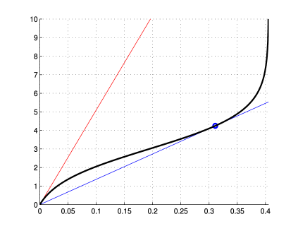
Figure 1: Solving equation $\alpha t=f_{k,n}(t)$ when $k<n/2$. The black curve is $y=f_{k,n}(t)$. The blue line is $y=\tilde{\alpha}t$ where $\tilde{\alpha}=\alpha(k,n)$ and the red line is $y=(n+1)t$.

Let us investigate the function $t\mapsto f_{k,n}(t)$ in more detail. We compute

$$f_{k,n}^{\prime}(t)= \frac{a}{{\mathrm{e}}^{t}-a}+\frac{b}{b-{\mathrm{e}}^{t}},$$

$$f_{k,n}^{\prime\prime}(t)= \left[-\frac{a}{({\mathrm{e}}^{t}-a)^{2}}+\frac{b}{(b-{\mathrm{e}}^{t})^{2}}\right]{\mathrm{e}}^{t}=\frac{(b-a){\mathrm{e}}^{t}({\mathrm{e}}^{2t}-ab)}{({\mathrm{e}}^{t}-a)^{2}(b-{\mathrm{e}}^{t})^{2}}.$$

From these equations, we obtain the following facts:

• $f_{k,n}(t)$ is an increasing function and $f_{k,n}(t)\to+\infty$ as $t\uparrow\ln(b)$;

• $f_{k,n}(0)=0$ and $f_{k,n}^{\prime}(0)=n+1$;

• $f_{k,n}(t)$ is concave for $t\in(\ln(a),\tilde{t})$ and convex for $t\in(\tilde{t},\ln(b))$, where $\tilde{t}:=\ln(ab)/2$;

• $f_{k,n}^{\prime\prime}(0)=(2k-n)(n+1)$;

• The inflection point $\tilde{t}$ satisfies $\tilde{t}\leq 0$ if $k\geq n/2$ and $\tilde{t}>0$ if $k<n/2$.

• For all $t\in(\ln(a),\ln(b))$ we have $f_{k,n}^{\prime}(t)\geq f_{k,n}^{\prime}(\tilde{t})=\frac{\sqrt{b}+\sqrt{a}}{\sqrt{b}-\sqrt{a}}>1$.

Let us first consider the case when $k<n/2$. Then the function $t\mapsto f_{k,n}(t)$ is concave on $(0,\tilde{t})$ and convex on $(\tilde{t},\ln(b))$. The graph of $f_{k,n}(t)$ is shown in Figure 1. Note that there exists a unique $\tilde{\alpha}(n,k)$ such that the straight line $y=\tilde{\alpha}t$ is tangent to $y=f_{k,n}(t)$ at some point $\tilde{t}$ (see the blue line in Figure 1). Since $f_{k,n}(0)=n+1$ and $f_{k,n}(t)$ is an increasing function, we see that $\tilde{\alpha}<n+1$, and item (vi) above shows that $\tilde{\alpha}>1$. It is clear that: for $\alpha>\tilde{\alpha}$ there is a solution $t_{2}(\alpha)$ to (29) that is an increasing function of $\alpha$; for $\alpha\in(\tilde{\alpha},n+1)$ there is another solution $t_{1}(\alpha)<\tilde{t}<t_{2}(\alpha)$ that is decreasing in $\alpha$; there are no other solutions to (29). This demonstrates both the existence and uniqueness of equilibria satisfying (ii) and (iii) of Theorem 3.3 respectively.

When $k\geq n/2$ the situation is simpler, as the function $t\mapsto f_{k,n}(t)$ is convex on $(0,\ln(b))$. Since $f_{k,n}^{\prime}(0)=n+1$ we see that for every $\alpha>n+1$ there exists a unique positive solution to (29), and that this solution is increasing in $\alpha$. See Figure 2. Finally, note that when $k=1$, $t\uparrow\log(b)$ as $\alpha\uparrow\infty$ implies that $v(n-1)/(1-v)\uparrow b=2$ which in turn implies that $v\uparrow 2/(n+1)$. ∎

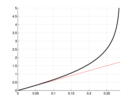
Figure 2: Solving equation $\alpha t=f_{k,n}(t)$ when $k\geq n/2$. The black curve is $y=f_{k,n}(t)$. The red line is $y=(n+1)t$.

For $\vec{v}\in\mathbb{R}^{n}$ and $a>0$, write $\vec{v}^{a}=(v_{1}^{a},\dots,v_{n}^{a})$, so that e.g. $((v)_{k},(u)_{n-k})^{a}=((v^{a})_{k},(u^{a})_{n-k})$.

Lemma 3.6.

Assume $\vec{v}=((v)_{k},(u)_{n-k})\in\mathcal{E}_{\alpha}$ for some $1\leq k\leq n-1$ and $v>u$. Let $\eta=kv^{\alpha}+(n-k)u^{\alpha}$ and $\xi=\alpha(n+1)^{-1}\eta^{-2}$. Then $\vec{v}\in\mathcal{S}_{\alpha}$ (critical if equality holds below) if and only if

$$k=1 \quad\qquad\text{and}\quad\qquad\xi(uv)^{\alpha-1}<1,\quad\text{or}$$

$$k\geq 2 \quad\qquad\text{and}\quad\qquad v<\frac{\alpha}{(\alpha-1)(n+1)}.$$

Proof.

The matrix ${\bf D}$ of partial derivatives has entries

$$D_{ii}= -1+\xi\times\begin{cases}v^{\alpha-1}\left((k-1)v^{\alpha}+(n-k)u^{\alpha}\right)&\text{ if }i\leq k,\\ u^{\alpha-1}\left(kv^{\alpha}+(n-k-1)u^{\alpha}\right)&\text{ if }i>k,\end{cases}$$

$$= -1+\xi\times\begin{cases}v^{\alpha-1}\eta-v^{2\alpha-1}&\text{ if }i\leq k,\\ u^{\alpha-1}\eta-u^{2\alpha-1}&\text{ if }i>k,\end{cases}$$

$$D_{ij}= -\xi\times\begin{cases}v^{2\alpha-1}&\text{ if }i,j\leq k,\\ v^{\alpha}u^{\alpha-1}&\text{ if }i\leq k<j,\\ v^{\alpha-1}u^{\alpha}&\text{ if }j\leq k<i,\\ u^{2\alpha-1}&\text{ if }i,j>k.\end{cases}$$

Let

$$\vec{x}= \vec{v}^{\alpha},\quad\text{and}\quad\vec{w}=-\xi\vec{v}^{\alpha-1}.$$ (30)

Let ${\bf Z}$ be a diagonal matrix with $Z_{ii}=D_{ii}+z_{i}$, where $\vec{z}=-\lambda\vec{1}+\xi\vec{v}^{2\alpha-1}$. Then

$$Z_{ii}=-(1+\lambda)+\xi\eta\begin{cases}v^{\alpha-1},&\text{ if }i\leq k,\\ u^{\alpha-1},&\text{ if }i>k,\end{cases}$$

and ${\bf D}-\lambda{\bf I}={\bf Z}+\vec{x}\vec{w}^{\mathrm{T}}$. It follows from Lemma 2.1 that

$$\det({\bf D}-\lambda{\bf I})= \det({\bf Z})+\vec{w}^{\mathrm{T}}\mathrm{adj}({\bf Z})\vec{x}$$

$$= Z_{1,1}^{k}Z_{n,n}^{n-k}-\xi v^{2\alpha-1}kZ_{1,1}^{k-1}Z_{n,n}^{n-k}-\xi u^{2\alpha-1}(n-k)Z_{1,1}^{k}Z_{n,n}^{n-k-1}$$

$$= Z_{1,1}^{k-1}Z_{n,n}^{n-k-1}\left(Z_{1,1}Z_{n,n}-\xi v^{2\alpha-1}kZ_{n,n}-\xi u^{2\alpha-1}(n-k)Z_{1,1}\right).$$

After a lot of simplifying, using the definition of $\eta$ and that $kv+(n-k)u=1$ we get that the term in brackets is zero if and only if

$$(1+\lambda)^{2}-(1+\lambda)\xi(uv)^{\alpha-1}=0,$$

i.e. if and only if $\lambda=-1$ or $\lambda=-1+\xi(uv)^{\alpha-1}$. The latter is $<0$ precisely when $\xi(uv)^{\alpha-1}<1$.

If $k>1$ then we also have an eigenvalue when $Z_{1,1}=0$, for which $\lambda=-1+\xi\eta v^{\alpha-1}$ is negative when $\xi\eta v^{\alpha-1}<1$. Similarly if $n-k>1$ then we also have an eigenvalue when $Z_{n,n}=0$ for which $\lambda=-1+\xi\eta u^{\alpha-1}$ is negative when $\xi\eta u^{\alpha-1}<1$.

Since $u<v$ we have that $\xi\eta u^{\alpha-1}<1$ if $\xi\eta v^{\alpha-1}<1$. Next,

$$\eta= u^{\alpha-1}(kv(v/u)^{\alpha-1}+(n-k)u)>u^{\alpha-1}(kv+(n-k)u)=u^{\alpha-1}.$$

This implies that $\xi(uv)^{\alpha-1}<1$ if $\xi\eta v^{\alpha-1}<1$. Similarly $v^{\alpha-1}>\eta$ so $\xi\eta u^{\alpha-1}<1$ when $\xi(uv)^{\alpha-1}<1$. Therefore, we have proved that the equilibrium with $k=1$ is linearly stable if and only if $\xi(uv)^{\alpha-1}<1$ and the equilibrium with $k\geq 2$ is linearly stable if and only if $\xi\eta v^{\alpha-1}<1$. Since $v$ satisfies

$$v=\frac{1}{n+1}+\frac{1}{n+1}\times\frac{v^{\alpha}}{kv^{\alpha}+(n-k)u^{\alpha}}=\frac{1}{n+1}+\frac{\xi\eta v^{\alpha}}{\alpha},$$

the condition $\xi\eta v^{\alpha-1}<1$ is equivalent to $v<\frac{\alpha}{(\alpha-1)(n+1)}$. ∎

Remark: The proof of Lemma 3.6 shows that if $k\geq 2$ and $((v)_{k},(u)_{n-k})\in\mathcal{S}_{\alpha}$ then $\xi(uv)^{\alpha-1}<1$. This observation will be useful for us later, when we investigate the stability of these equilibria.

Lemma 3.7.

Assume that $((v)_{k},(u)_{n-k})\in\mathcal{E}_{\alpha}$ with $v>u$ and $\xi$ and $\eta$ are defined as in Lemma 3.6. Then the condition $\xi(uv)^{\alpha-1}<1$ is equivalent to $\partial v/\partial\alpha>0$.

Proof.

We use the same notation as in the proof of Lemma 3.5, that is $t=\ln(v/u)$. Taking the derivative $\partial/\partial\alpha$ of both sides of equation (26) we obtain, with $t^{\prime}=\frac{{\textnormal{d}}t}{{\textnormal{d}}\alpha}$,

$$\frac{{\mathrm{e}}^{t}t^{\prime}}{(n+k({\mathrm{e}}^{t}-1))^{2}}=\frac{1}{n+1}\cdot\frac{{\mathrm{e}}^{\alpha t}(t+\alpha t^{\prime})}{(n-k+k{\mathrm{e}}^{\alpha t})^{2}}.$$

Since $t>0$ the above equation gives us

$$\frac{{\mathrm{e}}^{t}t^{\prime}}{(n+k({\mathrm{e}}^{t}-1))^{2}}>\frac{\alpha}{n+1}\cdot\frac{{\mathrm{e}}^{\alpha t}t^{\prime}}{(n-k+k{\mathrm{e}}^{\alpha t})^{2}}.$$

Rewriting this inequality in terms of $u$ and $v$ (recall that $u=1/(n+k({\mathrm{e}}^{t}-1))$ and ${\mathrm{e}}^{t}=v/u$) we obtain

$$uvt^{\prime}>\frac{\alpha}{n+1}\cdot\frac{(uv)^{\alpha}}{(kv^{\alpha}+(n-k)u^{\alpha})^{2}}t^{\prime}$$

which is equivalent to

$$t^{\prime}(\xi(uv)^{\alpha-1}-1)<0.$$

Therefore, $\xi(uv)^{\alpha-1}<1$ if and only if $t^{\prime}>0$, which is equivalent to $\partial v/\partial\alpha>0$ since $t=\log(v/u)$ and $u=(1-kv)/(n-k)$. ∎

Proof of Theorems 3.2 and 3.3. The fact that $(1/n)_{n}\in\mathcal{S}_{\alpha}$ if and only if $\alpha<n+1$ is part (iii) of Corollary 1.19. By Lemma 3.4 all other equilibria are of the form $((v)_{k},(u)_{n-k})$ for some $v>u$, $1\leq k\leq n-1$.

If $n=2$ then $k=1\geq n/2$, and we have by Lemma 3.5 that there exists an (unique) equilibrium of the form $((v)_{k},(u)_{n-k})$ with $v>u$ if and only if $\alpha>n+1$, and that $v(\alpha)$ is increasing to $2/3$. This proves Theorem 3.2.

For $n>2$, if $k=1$ and $\alpha\in(\tilde{\alpha}(1,n),n+1)$ we have by Lemma 3.5 that there exist two equilibria of the form $(v,(u)_{n-1})$, one of which has $\partial v/\partial\alpha<0$ and the other $\partial v/\partial\alpha>0$. Lemmas 3.6 and 3.7 tell us that linear stability is equivalent to $\partial v/\partial\alpha>0$, so this shows that only one of these two equilibria is linearly stable. When $\alpha>n+1$ we have a unique equilibrium of the form $(v,(u)_{n-1})$, and since $\partial v/\partial\alpha>0$ it is linearly stable.

Next, let us consider the equilibria corresponding to $k>1$. First, assume that $k\geq n/2$ or $k<n/2$ and $\alpha>n+1$. Then we have only one such equilibrium, which exists for $\alpha>n+1$. However, if $\alpha>n+1$ then $\alpha/((\alpha-1)(n+1))<1/n$, and Lemma 3.6 tells us that such an equilibrium can not be linearly stable (since $v>u$ implies $v>1/n$).

Finally, let us consider the case $k<n/2$ and $\alpha\in(\alpha(k,n),n+1)$. In this case we have two equilibria, corresponding to two solutions of equation $\alpha t=f_{k,n}(t)$ (see Figure 1). Let us denote these equilibria

$$\vec{v}^{\scriptscriptstyle(1)}=\vec{v}^{\scriptscriptstyle(1)}(\alpha)=((v^{\scriptscriptstyle(1)})_{k},(u^{\scriptscriptstyle(1)})_{n-k})$$

and similarly for $\vec{v}^{\scriptscriptstyle(2)}=\vec{v}^{\scriptscriptstyle(2)}(\alpha)$. We assume that $v^{\scriptscriptstyle(1)}<v^{\scriptscriptstyle(2)}$. From the proof of Lemma 3.5 we know that $v^{\scriptscriptstyle(1)}$ is a decreasing function of $\alpha$ while $v^{\scriptscriptstyle(2)}$ is an increasing function of $\alpha$.

From the remark on page 3.2 and Lemma 3.7, $\vec{v}^{\scriptscriptstyle(1)}$ can not be linearly stable since $v^{\scriptscriptstyle(1)}(\alpha)$ is decreasing in $\alpha$.

Let us consider the equilibrium $\vec{v}^{\scriptscriptstyle(2)}$. If this equilibrium is stable, then from Lemma 3.6, we find that $v^{\scriptscriptstyle(2)}<\alpha/((\alpha-1)(n+1))$. Since $v^{\scriptscriptstyle(1)}<v^{\scriptscriptstyle(2)}$, we see that $v^{\scriptscriptstyle(1)}$ also satisfies the condition $v^{\scriptscriptstyle(1)}<\alpha/((\alpha-1)(n+1))$, therefore $\vec{v}^{\scriptscriptstyle(1)}$ must be a stable equilibrium due to Lemma 3.6. Thus we have arrived at a contradiction (since we know that $\vec{v}^{\scriptscriptstyle(1)}$ can not be linearly stable), and we conclude that $\vec{v}^{\scriptscriptstyle(2)}$ is not linearly stable. ∎

3.3 Triangle graph

Consider a WARM triangle graph, under Condition $(\alpha)$. Equations (3) give us the following

$$v_{1} = \frac{1}{3}\frac{v_{1}^{\alpha}}{v_{1}^{\alpha}+v_{2}^{\alpha}}+\frac{1}{3}\frac{v_{1}^{\alpha}}{v_{1}^{\alpha}+v_{3}^{\alpha}},$$

$$v_{2} = \frac{1}{3}\frac{v_{2}^{\alpha}}{v_{2}^{\alpha}+v_{3}^{\alpha}}+\frac{1}{3}\frac{v_{2}^{\alpha}}{v_{1}^{\alpha}+v_{2}^{\alpha}},$$ (31)

$$v_{3} = \frac{1}{3}\frac{v_{3}^{\alpha}}{v_{1}^{\alpha}+v_{3}^{\alpha}}+\frac{1}{3}\frac{v_{3}^{\alpha}}{v_{2}^{\alpha}+v_{3}^{\alpha}}.$$

From now on we will list $(v_{1},v_{2},v_{3})$ in the decreasing order: $v_{1}\geq v_{2}\geq v_{3}$.

Theorem 3.8 (Equilibira and stability for WARM triangle graph).

The only equilibria for the WARM triangle graph are given by

• $(1/3,1/3,1/3)$, for all $\alpha>1$;

• $(1/2,1/2,0)$, for all $\alpha>1$;

• $(v,u,0)$ for $\alpha>3$, where $v>u$ and $v(\alpha)$ increases from $v(3+)=1/2$ to $v(+\infty)=2/3$ (here $(v,u)$ is an equilibrium for the line/star graph with two edges, see Theorem 3.2);

• $(v,v,u)$, for $\alpha\in(1,4/3]$, where $v>u$ and $v(\alpha)$ decreases from $v(1+)=1/2$ to $v(4/3-)=1/3$.

• $(v,u,u)$, for $\alpha\geq 4/3$, where $v>u$ and $v(\alpha)$ increases from $v(4/3+)=1/3$ to $v(+\infty)=2/3$;

Their stability properties are listed below:

Equilibrium (i) is linearly stable if and only if $$\alpha<4/3$$,

Equilibrium (ii) is linearly stable if and only if $$\alpha<3$$,

Equilibrium (iii) is linearly stable for all $$\alpha>3$$,

Equilibria (iv) and (v) are not linearly stable,

The equilibria are critical if and only if equality holds in the above.

The proof will be completed by a sequence of lemmas.

Lemma 3.9.

There exist equilibria described in items (iv) and (v) in Theorem 3.8.

Proof.

Let us consider an equilibrium $(v,u,u)$ with $v>u$. Let us denote $v/u={\mathrm{e}}^{t}$, note that $t>0$. From the condition $v+2u=1$ we find that $u=(2+{\mathrm{e}}^{t})^{-1}$. Then equation (2) in (3.3) gives us

$$\frac{1}{2+{\mathrm{e}}^{t}}=\frac{1}{6}+\frac{1}{3}\cdot\frac{1}{1+{\mathrm{e}}^{\alpha t}},$$ (32)

which can be rewritten in the form

$${\mathrm{e}}^{\alpha t}=\frac{3{\mathrm{e}}^{t}}{4-{\mathrm{e}}^{t}},$$

which is equivalent to

$$h(t):=\ln\left(\frac{3}{4-{\mathrm{e}}^{t}}\right)=(\alpha-1)t.$$ (33)

One can check that the function $h(t)$ is convex on $t\in(0,\log(4))$ and it satisfies $h(0)=0$ and $h^{\prime}(0)=1/3$, therefore (33) has a positive solution $t=t(\alpha)$ if and only if $\alpha>4/3$ (and this solution is necessarily unique). The graph of the function $t\mapsto h(t)$ is given in Figure 3. It is clear that ${\textnormal{d}}t/{\textnormal{d}}\alpha>0$ (see Figure 3), which implies that $v(\alpha)$ is an increasing function. Finally, $t(4/3)=0$ and $t(+\infty)=\ln(4)$, which gives us $v(4/3+)=1/3$ and $v(+\infty)=2/3$. This completes the proof of part (v) in Theorem 3.8.

Let us now consider an equilibrium $(v,v,u)$ with $v>u$. This case is equivalent to the previous one, except that now we have $u/v={\mathrm{e}}^{t}$ and $t<0$. One can check that $t$ also must satisfy (33), and that (33) has a negative solution if and only if $\alpha\in(1,4/3)$. This solution $t=t(\alpha)$ is unique, and it satisfies $\frac{{\textnormal{d}}t}{{\textnormal{d}}\alpha}>0$, which translates into the property that $v(\alpha)=1/(2+{\mathrm{e}}^{t})$ is a decreasing function. Since $t(4/3)=0$ and $t(1)=-\infty$ we see that $v(1+)=1/2$ and $v(4/3-)=1/3$. ∎

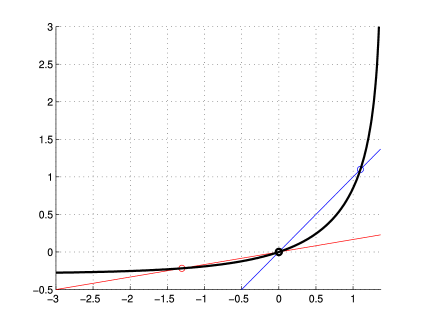
Figure 3: Finding equilibriums of the form $(v,u,u)$ and $(v,v,u)$. The black curve is the graph of the function $y=h(t)=\ln(3/(4-\exp(t)))$, the straight lines correspond to graphs of the functions $y=(\alpha-1)t$ for $\alpha=2$ (blue) and $\alpha=7/6$ (red).

Lemma 3.10.

For $\alpha\in(1,4/3)$, there are no equilibria other than (i)-(v) of Theorem 3.8.

Proof.

Assume that $(v,u,0)$ is an equilibrium. Then $(v,u)$ is an equilibrium for the line graph with two edges, and Theorem 3.2 shows that for $\alpha\in(1,3]$ the only such equilibrium is $(1/2,1/2)$, and for $\alpha>3$ there are two such equilibria, $(1/2,1/2,0)$ and $(v,1-v,0)$. This shows that there do not exist any other equilibria of the form $(v,1-v,0)$. Let us consider $(v_{1},v_{2},v_{3})$, where $v_{1}\geq v_{2}\geq v_{3}>0$. We will show that if $\alpha\in(1,4/3)$ and $(v_{1},v_{2},v_{3})$ is an equilibrium, then necessarily $v_{1}=v_{2}$. Assume $v_{1}>v_{2}$. We introduce the new variables $s>0$ and $a\geq 1$

$$\left(\frac{v_{2}}{v_{1}}\right)^{\alpha}={\mathrm{e}}^{-s},\qquad\quad\left(\frac{v_{2}}{v_{3}}\right)^{\alpha}=a.$$

Dividing the second equation in (3.3) by the first one we get

$$\frac{v_{2}}{v_{1}}=\frac{\frac{1}{1+\left(\frac{v_{3}}{v_{2}}\right)^{\alpha}}+\frac{1}{1+\left(\frac{v_{1}}{v_{2}}\right)^{\alpha}}}{\frac{1}{1+\left(\frac{v_{2}}{v_{1}}\right)^{\alpha}}+\frac{1}{1+\left(\frac{v_{3}}{v_{1}}\right)^{\alpha}}}$$

In our new notation, this is equivalent to

$${\mathrm{e}}^{-\frac{s}{\alpha}}=\frac{\frac{1}{1+a^{-1}}+\frac{1}{1+{\mathrm{e}}^{s}}}{\frac{1}{1+{\mathrm{e}}^{-s}}+\frac{1}{1+a^{-1}{\mathrm{e}}^{-s}}}.$$

We rewrite the above equation as

$${\mathrm{e}}^{\scriptscriptstyle(1-\frac{1}{\alpha})s}=\frac{\frac{a}{1+a}+\frac{1}{1+{\mathrm{e}}^{s}}}{\frac{1}{1+{\mathrm{e}}^{s}}+\frac{a}{1+a{\mathrm{e}}^{s}}},$$

and this is equivalent to

$$\left(1-\frac{1}{\alpha}\right)s=\ln(1+2a+a{\mathrm{e}}^{s})+\ln(1+a{\mathrm{e}}^{s})-\ln(1+a+2a{\mathrm{e}}^{s})-\ln(1+a)=:f_{a}(s).$$ (34)

We will show that for all $a\geq 1$ and for all $\beta:=(1-1/\alpha)\in[0,1/4]$, the equation $f_{a}(s)=\beta s$, $s\geq 0$ has a unique solution $s=0$, which implies that $v_{1}=v_{2}$. We calculate

$$f_{a}^{\prime}(s)=1-\frac{1+2a}{1+2a+a{\mathrm{e}}^{s}}-\frac{1}{1+a{\mathrm{e}}^{s}}+\frac{1+a}{1+a+2a{\mathrm{e}}^{s}},$$

which shows that

$$4f_{a}^{\prime}(s)-1=\frac{6a^{3}{\mathrm{e}}^{3s}+3a^{2}(a+1){\mathrm{e}}^{2s}+(6a^{3}-8a^{2}-4a){\mathrm{e}}^{s}-2a^{2}-3a-1}{(1+2a+a{\mathrm{e}}^{s})(1+a{\mathrm{e}}^{s})(1+a+2a{\mathrm{e}}^{s})}.$$

Note that, for all $s>0$,

$$6a^{3}{\mathrm{e}}^{3s}+(3a^{3}-8a^{2}-4a){\mathrm{e}}^{s}>6a^{3}{\mathrm{e}}^{s}+(6a^{3}-8a^{2}-4a){\mathrm{e}}^{s}=4a{\mathrm{e}}^{s}(3a^{2}-2a-1)\geq 0,\;\;\;{\textnormal{for all}}\;a\geq 1,$$

and

$$3a^{2}(a+1){\mathrm{e}}^{2s}-2a^{2}-3a-1>3a^{3}+a^{2}-3a-1=(3a+1)(a^{2}-1)\geq 0,\;\;\;{\textnormal{for all}}\;a\geq 1.$$

Therefore we have proved that $f_{a}^{\prime}(s)>1/4$ for all $a\geq 1$ and all $s>0$. As a result, for all $\beta\in(0,1/4)$ it is true that the function $s\mapsto f_{a}(s)-\beta s$ is strictly increasing, and since $f_{a}(0)=0$ it shows that the only non-negative solution to $f_{a}(s)=\beta s$ is $s=0$. ∎

Lemma 3.11.

For $\alpha\geq 4/3$ there are no equilibria other than (i)-(v) of Theorem 3.8.

Proof.

We assume that $\alpha\geq 4/3$ and $v_{2}>v_{3}>0$, our goal is to show that this leads to a contradiction. We start by rewriting the second and the third equations in (3.3) as follows

$$\frac{3}{v_{2}^{\alpha-1}} = \frac{a+2b+c}{(a+b)(b+c)},$$

$$\frac{3}{v_{3}^{\alpha-1}} = \frac{a+b+2c}{(a+c)(b+c)},$$

where we have denoted $a=v_{1}^{\alpha}$, $b=v_{2}^{\alpha}$ and $c=v_{3}^{\alpha}$. Dividing the second equation by the first one we obtain

$$\left(\frac{v_{2}}{v_{3}}\right)^{\alpha-1}=\frac{(a+b+2c)(a+b)}{(a+2b+c)(a+c)}.$$

Some simple algebra shows that the above equation is equivalent to

$$\left(\frac{v_{2}}{v_{3}}\right)^{\alpha-1}-1=\frac{b^{2}-c^{2}}{(a+2b+c)(a+c)}.$$

Since $b^{2}-c^{2}=(b-c)(b+c)=(b/c-1)(b+c)c$, the previous equation can be rewritten as

$$\frac{v_{2}}{v_{3}}\times\frac{\left(\frac{v_{2}}{v_{3}}\right)^{\alpha-1}-1}{\left(\frac{v_{2}}{v_{3}}\right)^{\alpha}-1}=\frac{v_{2}}{v_{3}}\times\frac{(b+c)c}{(a+2b+c)(a+c)}.$$ (35)

Let us denote the expression in the left-hand side {resp. in the right-hand side} as $L$ {resp. $R$}. Our first goal is to prove that $L>1/4$. Let us denote $w=v_{2}/v_{3}$, note that $w>1$. Then

$$L:=w\frac{w^{\alpha-1}-1}{w^{\alpha}-1}=1-\frac{w-1}{w^{\alpha}-1}.$$ (36)

It is easy to check that for all $\alpha>1$ the function $z\mapsto(z^{\alpha}-1)/(z-1)$ is strictly increasing for $z\in(1,\infty)$, therefore we have

$$\frac{w^{\alpha}-1}{w-1}>\lim\limits_{z\to 1^{+}}\frac{z^{\alpha}-1}{z-1}=\alpha.$$

This implies $(w-1)/(w^{\alpha}-1)<1/\alpha$ and

$$L=1-\frac{w-1}{w^{\alpha}-1}>1-\frac{1}{\alpha}\geq 1/4.$$ (37)

Our second goal is to prove that $R\leq 1/4$. Let us denote $x=v_{2}/v_{1}$ and $y=v_{3}/v_{2}$, so that $v_{2}=xv_{1}$ and $v_{3}=xyv_{1}$. Note that the inequality $v_{1}\geq v_{2}>v_{3}>0$ implies $0<x\leq 1$ and $0<y<1$. We rewrite the right-hand side in (35) as

$$R:=\frac{v_{2}}{v_{3}}\times\frac{(b+c)c}{(a+2b+c)(a+c)} = \frac{v_{2}(v_{2}^{\alpha}+v_{3}^{\alpha})v_{3}^{\alpha-1}}{(v_{1}^{\alpha}+2v_{2}^{\alpha}+v_{3}^{\alpha})(v_{1}^{\alpha}+v_{3}^{\alpha})}$$

$$= \frac{x^{2\alpha}y^{\alpha-1}(1+y^{\alpha})}{(1+x^{\alpha}(2+y^{\alpha}))(1+x^{\alpha}y^{\alpha})}=:f(x,y).$$

First we check that for all $q>0$ the function $z\mapsto z^{2}/((1+z(2+q))(1+zq))$ is increasing for $z>0$, thus

$$\sup\limits_{0<z\leq 1}\frac{z^{2}}{(1+z(2+q))(1+zq)}=\frac{z^{2}}{(1+z(2+q))(1+zq)}\Big{|}_{z=1}=\frac{1}{(3+q)(1+q)}.$$

Therefore from the above identity and (3.3) we obtain

$$R\leq\sup\limits_{0<t<1}\left[\sup\limits_{0<s\leq 1}f(s,t)\right] = \sup\limits_{0<t<1}t^{\alpha-1}(1+t^{\alpha})\left[\sup\limits_{0<s\leq 1}\frac{s^{2\alpha}}{(1+s^{\alpha}(2+t^{\alpha}))(1+s^{\alpha}t^{\alpha})}\right]$$ (39)

$$= \sup\limits_{0<t<1}\frac{t^{\alpha-1}}{3+t^{\alpha}}.$$

Consider the function $g(t):=t^{\alpha-1}/(3+t^{\alpha})$. We compute

$$\frac{{\textnormal{d}}g(t)}{{\textnormal{d}}t}=\frac{t^{\alpha-2}(3(\alpha-1)-t^{\alpha})}{(3+t^{\alpha})^{2}}.$$

Since $3(\alpha-1)\geq 1$ for $\alpha\geq 4/3$, we see that ${\textnormal{d}}g(t)/{\textnormal{d}}t>0$ for $0<t<1$, thus $g(t)$ is increasing for $t\in(0,1)$ and

$$\sup\limits_{\begin{subarray}{c}0<s\leq 1\\ 0<t<1\end{subarray}}f(s,t)=\sup\limits_{0<t<1}\frac{t^{\alpha-1}}{3+t^{\alpha}}=\frac{t^{\alpha-1}}{3+t^{\alpha}}\Big{|}_{t=1}=\frac{1}{4}.$$

The above equation combined with (35), (37) and (39) imply $1/4<L=R\leq 1/4$. This shows that our initial assumption $v_{2}>v_{3}>0$ can not be true, therefore $v_{3}=0$ or $v_{2}=v_{3}$. ∎

Lemma 3.12.

Let us define

$$\eta:=\frac{\alpha(uv)^{\alpha}}{3(u^{\alpha}+v^{\alpha})^{2}}.$$

An equilibrium of the form $(v,u,u)$ or $(u,u,v)$ for $v>u$ is linearly stable if and only if both $\eta<uv$ and $\eta<u-\frac{\alpha}{6}$.

Proof.

Assume that $(v_{1},v_{2},v_{3})=(v,u,u)$ and $v\neq u$. The Jacobian matrix is of the form

$${\bf D}=\begin{pmatrix}-1+\frac{2\eta}{v}&-\frac{\eta}{u}&-\frac{\eta}{u}\\ -\frac{\eta}{v}&-1+\frac{\alpha}{12u}+\frac{\eta}{u}&-\frac{\alpha}{12u}\\ -\frac{\eta}{v}&-\frac{\alpha}{12u}&-1+\frac{\alpha}{12u}+\frac{\eta}{u}\end{pmatrix}.$$ (40)

One can check that

$${\textnormal{det}}({\bf D}-\lambda{\bf I})=-(\lambda+1)\left(\lambda+1-\frac{\eta}{uv}(v+2u)\right)\left(\lambda+1-\frac{\alpha+6\eta}{6u}\right).$$

Since $v+2u=1$ we see that the eigenvalues are

$$\lambda_{1}=-1,\;\;\;\lambda_{2}=-1+\frac{\eta}{uv},\;\;\;\lambda_{3}=-1+\frac{\alpha+6\eta}{6u}.$$

∎

Lemma 3.13.

The equilibrium of Theorem 3.8(iv) is not linearly stable.

Proof.

Assume that $(v,u,u)$ is an equilibrium, such that $v>u$ and $\alpha>4/3$. In order to show that $(v,u,u)$ is not a linearly stable equilibrium it is enough to prove that that $\eta>u-\alpha/6$ (see Lemma 3.12). Define $r=v/u$. The condition $\eta>u-\alpha/6$ is equivalent to

$$\frac{1}{2}+\frac{r^{\alpha}}{(1+r^{\alpha})^{2}}>\frac{3}{\alpha(2+r)}.$$

This inequality is obvious if $\alpha>2$, so we only need to consider $\alpha\in(4/3,2]$. Let us introduce the new variable $z=r^{\frac{\alpha}{2}}-1$, so that $r=(1+z)^{\frac{2}{\alpha}}$. With this notation, we need to prove that for all $\alpha\in(4/3,2]$ and all $z>0$

$$\frac{1}{2}+\frac{(1+z)^{2}}{(1+(1+z)^{2})^{2}}>\frac{3}{\alpha(2+(1+z)^{\frac{2}{\alpha}})}.$$

For all $\alpha\in(4/3,2]$ and all $z>0$ we have $(1+z)^{\frac{2}{\alpha}}\geq 1+z$, therefore

$$\frac{3}{\alpha(2+(1+z)^{\frac{2}{\alpha}})}\leq\frac{3}{\alpha(3+z)}<\frac{9}{4(3+z)}.$$

So it is enough to show that for all $z>0$

$$\frac{1}{2}+\frac{(1+z)^{2}}{(1+(1+z)^{2})^{2}}>\frac{9}{4(3+z)}.$$

Multiplying both sides by $(1+(1+z)^{2})^{2}(3+z)$ and simplifying the resulting expressions, we obtain that the above inequality is equivalent to

$$2z^{5}+5z^{4}+8z^{3}+12z^{2}+12z>0\;\;\;{\textnormal{for all}}\;z>0,$$

which is obviously true. ∎

Lemma 3.14.

The equilibrium of Theorem 3.8(v) is not linearly stable.

Proof.

We will show that the first condition of Lemma 3.12 is not satisfied, that is $\eta>uv$ for all $\alpha>4/3$.

Assume that $(v,v,u)$ is an equilibrium. Consider the same parameterization as in the proof of Lemma 3.9: $u/v={\mathrm{e}}^{t}$, $v=(2+{\mathrm{e}}^{t})^{-1}$. Note that $t<0$ and from the proof of Lemma 3.9 we know that $\frac{{\textnormal{d}}t}{{\textnormal{d}}\alpha}>0$. We consider $t$ as a function of $\alpha$. Equation (32) gives us

$$\frac{{\textnormal{d}}}{{\textnormal{d}}\alpha}\left[\frac{1}{2+{\mathrm{e}}^{t}}\right]=\frac{{\textnormal{d}}}{{\textnormal{d}}\alpha}\left[\frac{1}{6}+\frac{1}{3}\cdot\frac{1}{1+{\mathrm{e}}^{\alpha t}}\right],$$

which is equivalent to

$$\frac{{\mathrm{e}}^{t}t^{\prime}}{(2+{\mathrm{e}}^{t})^{2}}=\frac{1}{3}\cdot\frac{{\mathrm{e}}^{\alpha t}(t+\alpha t^{\prime})}{(1+{\mathrm{e}}^{\alpha t})^{2}},$$

where $t^{\prime}:=\frac{{\textnormal{d}}t}{{\textnormal{d}}\alpha}$. Since $t<0$ and $t^{\prime}>0$,

$$\frac{{\mathrm{e}}^{t}}{(2+{\mathrm{e}}^{t})^{2}}<\frac{1}{3}\cdot\frac{{\mathrm{e}}^{\alpha t}\alpha}{(1+{\mathrm{e}}^{\alpha t})^{2}}.$$

Since ${\mathrm{e}}^{t}=u/v$ and $(2+{\mathrm{e}}^{t})^{-1}=v$, the above inequality gives us

$$uv<\frac{\alpha(uv)^{\alpha}}{3(u^{\alpha}+v^{\alpha})^{2}}.$$

Applying Lemma 3.12, we conclude that $(v,v,u)$ is not a linearly stable equilibrium. ∎

3.4 Whisker graph

Since we already understand the star-graph setting, let us in this section restrict our attention to whisker graphs that are not star graphs.

For the $(r,s)$-whisker graph (with $r+1+s=n$), $\vec{v}\in\mathcal{E}_{\alpha}$ if and only if $\vec{v}$ satisfies (for all $i=1,\dots,n$)

$$0=F(\vec{v})_{i}=-v_{i}+\frac{1}{n+1}\begin{cases}1+\frac{v_{i}^{\alpha}}{\delta_{r}},&i\leq r,\\ v_{r+1}^{\alpha}\left[\frac{1}{\delta_{r}}+\frac{1}{\delta_{s}}\right],&i=r+1,\\ 1+\frac{v_{i}^{\alpha}}{\delta_{s}},&r+2\leq i\leq n,\end{cases}$$ (41)

where $\delta_{r}=\sum_{i=1}^{r+1}v_{i}^{\alpha}$ and $\delta_{s}=\sum_{i=r+1}^{n}v_{i}^{\alpha}$. Fixing $\delta_{r}$ and repeating the proof of Lemma 3.4 with $f$ given by (24), we have that for any equilibrium $\vec{v}$ on a whisker graph, $\{v_{1},\dots,v_{r}\}$ has at most 2 distinct elements (only one element when $\delta_{r}\notin\frac{(\alpha-1)}{(n+1)^{\alpha}}(1,2^{\alpha})$). Similarly $\{v_{r+2},\dots,v_{n}\}$ has at most 2 distinct elements (only one element when $\delta_{s}\notin\frac{(\alpha-1)}{(n+1)^{\alpha}}(1,2^{\alpha})$). From this we obtain the following lemma:

Lemma 3.15.

For all $\alpha>1$, all equilibria for a whisker graph are of the form

$$((v)_{k_{r}},(u)_{r-k_{r}},v_{r+1},(v^{\prime})_{k_{s}},(u^{\prime})_{s-k_{s}}).$$ (42)

Note that $v_{r+1}\geq 0$ and all other entries are bounded above and below by $2/(n+1)$ and $1/(n+1)$, respectively. For such $\vec{v}$, we have that $\delta_{r}=k_{r}v^{\alpha}+(r-k_{r})u^{\alpha}+v_{r+1}^{\alpha}$ and similarly $\delta_{s}=k_{s}(v^{\prime})^{\alpha}+(s-k_{s})(u^{\prime})^{\alpha}+v_{r+1}^{\alpha}$.

Letting $\xi_{r}=\frac{\alpha}{(n+1)\delta_{r}^{2}}$ and $\xi_{s}=\frac{\alpha}{(n+1)\delta_{s}^{2}}$ we have that

$$D_{i,i}= -1+\frac{\alpha}{n+1}\begin{cases}v_{i}^{\alpha-1}\left[\frac{\delta_{r}-v_{i}^{\alpha}}{\delta_{r}^{2}}\right],&i\leq r,\\ v_{r+1}^{\alpha-1}\left[\frac{(\delta_{r}-v_{r+1}^{\alpha})}{\delta_{r}^{2}}+\frac{(\delta_{s}-v_{r+1}^{\alpha})}{\delta_{s}^{2}}\right],&i=r+1,\\ v_{i}^{\alpha-1}\left[\frac{\delta_{s}-v_{i}^{\alpha}}{\delta_{s}^{2}}\right],&r+2\leq i\leq n.\end{cases}$$ (43)

$$= -1+\begin{cases}\xi_{r}v^{\alpha-1}(\delta_{r}-v^{\alpha}),&i\leq k_{r},\\ \xi_{r}u^{\alpha-1}(\delta_{r}-u^{\alpha}),&k_{r}+1\leq i\leq r,\\ \xi_{r}v_{r+1}^{\alpha-1}(\delta_{r}-v_{r+1}^{\alpha})+\xi_{s}v_{r+1}^{\alpha-1}(\delta_{s}-v_{r+1}^{\alpha}),&i=r+1\\ \xi_{s}(v^{\prime})^{\alpha-1}(\delta_{s}-(v^{\prime})^{\alpha}),&r+2\leq i\leq r+2+k_{s},\\ \xi_{s}(u^{\prime})^{\alpha-1}(\delta_{s}-(u^{\prime})^{\alpha}),&r+2+k_{s}\leq i\leq n.\end{cases}$$

Moreover $D_{i,\ell}=0$ if $i\leq r$ and $\ell\geq r+2$ (or vice versa) and otherwise

$$D_{i,\ell}=-v_{i}^{\alpha}v_{\ell}^{\alpha-1}\begin{cases}\xi_{r},&i,\ell\leq r+1,i\neq\ell,\\ \xi_{s},&i,\ell\geq r+1,i\neq\ell.\end{cases}$$

Now ${\bf M}\equiv{\bf D}-\lambda{\bf I}$ is of the form

$${\bf M}=\begin{pmatrix}{\bf A}&\vline\,\vec{g}\,\vline&0\\ \hline\cr\vec{h}^{\mathrm{T}}&\vline\,a\,\vline&\vec{t}^{\mathrm{T}}\\ \hline\cr 0&\vline\,\vec{z}\,\vline&{\bf B}\end{pmatrix},$$

where ${\bf A}\in\mathbb{R}^{r\times r}$ has the same form as the matrix ${\bf D}-\lambda{\bf I}$ in the case of the star-graph on $r$ edges,

$$\vec{g}^{\mathrm{T}}=-\frac{\alpha v_{r+1}^{\alpha-1}}{(n+1)\delta_{r}^{2}}(v^{\alpha},\dots,v^{\alpha},u^{\alpha},\dots,u^{\alpha})\in\mathbb{R}^{r}$$

$$\vec{h}^{\mathrm{T}}=-\frac{\alpha v_{r+1}^{\alpha}}{(n+1)\delta_{r}^{2}}(v^{\alpha-1},\dots,v^{\alpha-1},u^{\alpha-1},\dots,u^{\alpha-1})\in\mathbb{R}^{r}$$

and $a=D_{r+1,r+1}-\lambda$ etc. We have that

$$\vec{g}= -\xi_{r}v_{r+1}^{\alpha-1}\vec{x}_{r},\qquad\quad\vec{h}=v_{r+1}^{\alpha}\vec{w}_{r},$$

where $\vec{x}_{r}$ and $\vec{w}_{r}$ are defined as in (30) (but with $\xi_{r}$ instead of $\xi$), i.e.,

$$\vec{x}_{r}^{\mathrm{T}}= (v^{\alpha},\dots,v^{\alpha},u^{\alpha},\dots,u^{\alpha}),\quad\text{ and }$$ (44)

$$\vec{w}_{r}^{\mathrm{T}}= -\xi_{r}(v^{\alpha-1},\dots,v^{\alpha-1},u^{\alpha-1},\dots,u^{\alpha-1}).$$ (45)

Similarly,

$$\vec{z}= -\xi_{s}v_{r+1}^{\alpha-1}\vec{x}^{\prime}_{s},\qquad\quad\vec{t}=v_{r+1}^{\alpha}\vec{w}^{\prime}_{s}.$$

Lemma 3.16.

The determinant of ${\bf M}$ is given by

$$\det({\bf M})= a\det({\bf A})\det({\bf B})-\left(\det({\bf B})\vec{h}^{\mathrm{T}}\mathrm{adj}({\bf A})\vec{g}+\det({\bf A})\vec{t}^{\mathrm{T}}\mathrm{adj}({\bf B})\vec{z}\right).$$ (46)

Proof.

Firstly note that $\det({\bf M})=\det({\bf H})$, where

$${\bf H}=\begin{pmatrix}{\bf A}&{\bf 0}&\vec{g}\\ {\bf 0}&{\bf B}&\vec{z}\\ \vec{h}^{\mathrm{T}}&\vec{t}^{\mathrm{T}}&a\end{pmatrix}.$$

Let ${\bf R}=\begin{pmatrix}{\bf A}&{\bf 0}\\ {\bf 0}&{\bf B}\end{pmatrix}$. Then using the block matrix form of ${\bf H}$,

$$\det({\bf H})= (a+1)\det({\bf R})-\det\left({\bf R}+{\vec{g}\choose\vec{z}}(\vec{h}^{\mathrm{T}},\vec{t}^{\mathrm{T}})\right).$$

Now by definition of $\mathrm{adj}$ we have that ${\bf R}\mathrm{adj}({\bf R})=\det({\bf R}){\bf I}$, from which it follows easily that for ${\bf R}$ of the form $\begin{pmatrix}{\bf A}&{\bf 0}\\ {\bf 0}&{\bf B}\end{pmatrix}$

$$\mathrm{adj}({\bf R})=\begin{pmatrix}\det({\bf B})\mathrm{adj}({\bf A})&{\bf 0}\\ {\bf 0}&\det({\bf A})\mathrm{adj}({\bf B})\end{pmatrix}$$

Combining this with Lemma 2.1, we arrive at

$$\det({\bf H})= (a+1)\det({\bf R})-\left(\det({\bf R})+(\vec{h}^{\mathrm{T}},\vec{t}^{\mathrm{T}})\mathrm{adj}({\bf R}){\vec{g}\choose\vec{z}}\right)$$

$$= a\det({\bf R})-\left(\det({\bf B})\vec{h}^{\mathrm{T}}\mathrm{adj}({\bf A})\vec{g}+\det({\bf A})\vec{t}^{\mathrm{T}}\mathrm{adj}({\bf B})\vec{z}\right).$$

But $\det({\bf R})=\det({\bf A})\det({\bf B})$, yielding (46). ∎

Now we know that ${\bf A}$ and ${\bf B}$ can be written in the form ${\bf A}={\bf Z}+\vec{x}_{r}\vec{w}^{\mathrm{T}}_{r}$ and ${\bf B}={\bf Z^{\prime}}+\vec{x}_{s}^{\prime}(\vec{w}^{\prime}_{s})^{\mathrm{T}}$ and where ${\bf Z}$ and ${\bf Z^{\prime}}$ are diagonal matrices with

$$Z_{ii}= -(1+\lambda)+\delta_{r}\xi_{r}\begin{cases}v^{\alpha-1},&i\leq k_{r},\\ u^{\alpha-1},&k_{r}<i\leq r,\end{cases}$$

$$Z^{\prime}_{ii}= -(1+\lambda)+\delta_{s}\xi_{s}\begin{cases}(v^{\prime})^{\alpha-1},&i\leq k_{s},\\ (u^{\prime})^{\alpha-1},&k_{s}<i\leq n-r-1,\end{cases}$$

for which $\mathrm{adj}({\bf Z})$ is easy to express. Indeed,

$$\det({\bf Z})= (-(1+\lambda)+\delta_{r}\xi_{r}v^{\alpha-1})^{k_{r}}(-(1+\lambda)+\delta_{r}\xi_{r}u^{\alpha-1})^{r-k_{r}},$$

$$\vec{w}_{r}^{\mathrm{T}}\mathrm{adj}({\bf Z})\vec{u}_{r}= -\xi_{r}\left(\sum_{i=1}^{k_{r}}v^{2\alpha-1}\left[(-(1+\lambda)+\delta_{r}\xi_{r}v^{\alpha-1})^{k_{r}-1}(-(1+\lambda)+\delta_{r}\xi_{r}u^{\alpha-1})^{r-k_{r}}\right]\right.$$

$$\quad+\left.\sum_{i=k_{r}+1}^{r}u^{2\alpha-1}\left[(-(1+\lambda)+\delta_{r}\xi_{r}u^{\alpha-1})^{k_{r}}(-(1+\lambda)+\delta_{r}\xi_{r}v^{\alpha-1})^{r-k_{r}-1}\right]\right),$$

and if both $k_{r}\geq 1$ and $r-k_{r}\geq 1$ this becomes

$$\vec{w}_{r}^{\mathrm{T}}\mathrm{adj}({\bf Z})\vec{u}_{r}= -\xi_{r}(-(1+\lambda)+\delta_{r}\xi_{r}v^{\alpha-1})^{k_{r}-1}(-(1+\lambda)+\delta_{r}\xi_{r}u^{\alpha-1})^{r-k_{r}-1}$$

$$\quad\Big{(}k_{r}v^{2\alpha-1}(-(1+\lambda)+\delta_{r}\xi_{r}u^{\alpha-1})+(r-k_{r})u^{2\alpha-1}(-(1+\lambda)+\delta_{r}\xi_{r}u^{\alpha-1})\Big{)}.$$

Similarly

$$\det({\bf Z^{\prime}})= (-(1+\lambda)+\delta_{s}\xi_{s}v^{\alpha-1})^{k_{s}}(-(1+\lambda)+\delta_{s}\xi_{s}(u^{\prime})^{\alpha-1})^{s-k_{s}},$$

$$\vec{w}_{s}^{\mathrm{T}}\mathrm{adj}({\bf Z^{\prime}})\vec{u}_{s}= -\xi_{s}\left(\sum_{i=1}^{k_{s}}(v^{\prime})^{2\alpha-1}\left[(-(1+\lambda)+\delta_{s}\xi_{s}(v^{\prime})^{\alpha-1})^{k_{s}-1}(-(1+\lambda)+\delta_{s}\xi_{s}(u^{\prime})^{\alpha-1})^{s-k_{s}}\right]\right.$$

$$\quad+\left.\sum_{i=k_{s}+1}^{s}(u^{\prime})^{\alpha-1}\left[(-(1+\lambda)+\delta_{s}\xi_{s}(u^{\prime})^{\alpha-1})^{k_{s}}(-(1+\lambda)+\delta_{s}\xi_{s}(v^{\prime})^{\alpha-1})^{s-k_{s}-1}\right]\right).$$

The question is whether we can handle the term of the form $\vec{h}^{\mathrm{T}}\mathrm{adj}({\bf A})\vec{g}$. However, again by Lemma 2.1,

$$\vec{h}^{\mathrm{T}}\mathrm{adj}({\bf A})\vec{g}=\det({\bf A}+\vec{g}\vec{h}^{\mathrm{T}})-\det({\bf A}),$$

and we know what to do with $\det({\bf A})$ as above. On the other hand, since ${\bf A}={\bf Z}+\vec{u}_{r}\vec{w}_{r}$ and $\vec{g}=-\xi_{r}v_{r+1}^{\alpha-1}\vec{u}_{r}$ and $\vec{h}=v_{r+1}^{\alpha}\vec{w}_{r}$,

$${\bf A}+\vec{g}\vec{h}^{\mathrm{T}}={\bf Z}+\vec{u}_{r}\vec{w}_{r}^{\mathrm{T}}-\xi_{r}v_{r+1}^{2\alpha-1}\vec{u}_{r}\vec{w}_{r}^{\mathrm{T}}={\bf Z}+(1-\xi_{r}v_{r+1}^{2\alpha-1})\vec{u}_{r}\vec{w}_{r}^{\mathrm{T}}.$$

Thus we can express the determinant of ${\bf A}+\vec{g}\vec{h}^{\mathrm{T}}$ as

$$\det({\bf A}+\vec{g}\vec{h}^{\mathrm{T}})= \det({\bf Z})+(1-\xi_{r}v_{r+1}^{2\alpha-1})\vec{w}_{r}^{\mathrm{T}}\mathrm{adj}({\bf Z})\vec{u}_{r}$$

$$= \det({\bf A})-\xi_{r}v_{r+1}^{2\alpha-1}\vec{w}_{r}^{\mathrm{T}}\mathrm{adj}({\bf Z})\vec{u}_{r},$$

since $\det({\bf A})=\det({\bf Z})+\vec{w}_{r}^{\mathrm{T}}\mathrm{adj}({\bf Z})\vec{u}_{r}$. Since we can do the same with the ${\bf B}$ terms we can write an expression for the determinant in terms of all these quantities.

Recall from (43) that

$$a= -(1+\lambda)+\frac{\alpha v_{r+1}^{\alpha-1}}{n+1}\left[\frac{(\delta_{r}-v_{r+1}^{\alpha})}{\delta_{r}^{2}}+\frac{(\delta_{s}-v_{r+1}^{\alpha})}{\delta_{s}^{2}}\right]$$

$$= -(1+\lambda)+v_{r+1}^{\alpha-1}\big{(}\xi_{r}(\delta_{r}-v_{r+1}^{\alpha})+\xi_{s}(\delta_{s}-v_{r+1}^{\alpha})\big{)},$$

where $\delta_{r}-v_{r+1}^{\alpha}=\sum_{i=1}^{r}v_{i}^{\alpha}$ and $\delta_{s}-v_{r+1}^{\alpha}=\sum_{i=r+2}^{n}v_{i}^{\alpha}$. From (46) and the above we have established the following lemma:

Lemma 3.17.

The determinant of ${\bf M}$ satisfies

$$\det({\bf M})= a\left[\det({\bf Z})+\vec{w}_{r}^{\mathrm{T}}\mathrm{adj}({\bf Z})\vec{u}_{r}\right]\left[\det({\bf Z^{\prime}})+\vec{w}_{s}^{\mathrm{T}}\mathrm{adj}({\bf Z^{\prime}})\vec{u}_{s}\right]$$ (47)

$$+\left[\det({\bf Z^{\prime}})+\vec{w}_{s}^{\mathrm{T}}\mathrm{adj}({\bf Z^{\prime}})\vec{u}_{s}\right]\left[\xi_{r}v_{r+1}^{2\alpha-1}\vec{w}_{r}^{\mathrm{T}}\mathrm{adj}({\bf Z})\vec{u}_{r}\right]$$ (48)

$$+\left[\det({\bf Z})+\vec{w}_{r}^{\mathrm{T}}\mathrm{adj}({\bf Z})\vec{u}_{r}\right]\left[\xi_{s}v_{r+1}^{2\alpha-1}\vec{w}_{s}^{\mathrm{T}}\mathrm{adj}({\bf Z^{\prime}})\vec{u}_{s}\right].$$ (49)

3.4.1 Special cases

If $v_{r+1}=0$ then $a=-(1+\lambda)$, the two terms (48) and (49) vanish and we recover the fact (see Theorem 1.22) that the case $v_{r+1}=0$ is linearly stable if and only if each of the remaining star graphs is linearly stable.

Let us now examine the completely symmetric case $r=s=k_{r}=k_{s}$, $v=v^{\prime}$.

Lemma 3.18.

For the symmetric whisker graph with $r=s=k_{r}=k_{s}$, $\vec{v}=((v)_{r},v_{r+1},(v)_{r})$ is a linearly stable equilibrium if and only if

$$\xi_{r}v_{r+1}^{\alpha-1}v^{\alpha-1}<1,\quad\text{and in the case $r>1$ also}\quad\delta_{r}\xi_{r}v^{\alpha-1}<1.$$

Proof.

We have that ${\bf Z}={\bf Z^{\prime}}$ etc., and thus

$$\det({\bf M})= a\left[\det({\bf Z})+\vec{w}_{r}^{\mathrm{T}}\mathrm{adj}({\bf Z})\vec{u}_{r}\right]^{2}$$

$$+2\left[\xi_{r}v_{r+1}^{2\alpha-1}\vec{w}_{r}^{\mathrm{T}}\mathrm{adj}({\bf Z})\vec{u}_{r}\right]\left[\det({\bf Z})+\vec{w}_{r}^{\mathrm{T}}\mathrm{adj}({\bf Z})\vec{u}_{r}\right]$$

$$= \left[\det({\bf Z})+\vec{w}_{r}^{\mathrm{T}}\mathrm{adj}({\bf Z})\vec{u}_{r}\right]\left(a\left[\det({\bf Z})+\vec{w}_{r}^{\mathrm{T}}\mathrm{adj}({\bf Z})\vec{u}_{r}\right]+2\left[\xi_{r}v_{r+1}^{2\alpha-1}\vec{w}_{r}^{\mathrm{T}}\mathrm{adj}({\bf Z})\vec{u}_{r}\right]\right).$$

Here $\det({\bf Z})=(-(1+\lambda)+\delta_{r}\xi_{r}v^{\alpha-1})^{r}$ and

$$\det({\bf Z})+\vec{w}_{r}^{\mathrm{T}}\mathrm{adj}({\bf Z})\vec{u}_{r}= (-(1+\lambda)+\delta_{r}\xi_{r}v^{\alpha-1})^{r}-r\xi_{r}v^{2\alpha-1}(-(1+\lambda)+\delta_{r}\xi_{r}v^{\alpha-1})^{r-1}$$

$$= (-(1+\lambda)+\delta_{r}\xi_{r}v^{\alpha-1})^{r-1}\left[(-(1+\lambda)+\delta_{r}\xi_{r}v^{\alpha-1})-r\xi_{r}v^{2\alpha-1}\right]$$

$$= (-(1+\lambda)+\delta_{r}\xi_{r}v^{\alpha-1})^{r-1}\left[-(1+\lambda)+\xi_{r}v^{\alpha-1}v_{r+1}^{\alpha}\right],$$

so

$$\lambda=\delta_{r}\xi_{r}v^{\alpha-1}-1,\quad\text{and}\quad\lambda=\xi_{r}v^{\alpha-1}v_{r+1}^{\alpha}-1$$

are eigenvalues, with the first of multiplicity $r-1$ (vanishing when $r=1$).

Next

$$a= -(1+\lambda)+v_{r+1}^{\alpha-1}\big{(}\xi_{r}(\delta_{r}-v_{r+1}^{\alpha})+\xi_{s}(\delta_{s}-v_{r+1}^{\alpha})\big{)}$$

$$= -(1+\lambda)+2rv_{r+1}^{\alpha-1}\xi_{r}v^{\alpha},$$

so

$$\det({\bf M})= \big{(}-(1+\lambda)+2rv_{r+1}^{\alpha-1}\xi_{r}v^{\alpha}\big{)}(-(1+\lambda)+\delta_{r}\xi_{r}v^{\alpha-1})^{r-1}\left[-(1+\lambda)+\xi_{r}v^{\alpha-1}v_{r+1}^{\alpha}\right]$$

$$-2r\xi_{r}v^{2\alpha-1}(-(1+\lambda)+\delta_{r}\xi_{r}v^{\alpha-1})^{r-1}\xi_{r}v_{r+1}^{2\alpha-1}$$

$$= (-(1+\lambda)+\delta_{r}\xi_{r}v^{\alpha-1})^{r-1}\big{(}1+\lambda\big{)}\left[(1+\lambda)-\xi_{r}v_{r+1}^{\alpha-1}v^{\alpha-1}\right],$$

where we have used $2rv+v_{r+1}=1$. The corresponding eigenvalues are

$$\lambda=\delta_{r}\xi_{r}v^{\alpha-1}-1,\quad\lambda=-1,\quad\text{and}\quad\lambda=\xi_{r}v_{r+1}^{\alpha-1}v^{\alpha-1}-1,$$

with the former not being present when $r=1$.∎

We are now ready to state our main result of this section:

Theorem 3.19.

On the symmetric whisker graph, with $r\geq 1$ there exists $\alpha(r)>1$ such that for any $\alpha>\alpha(r)$ there exist two equilibria of the form $((v)_{r},u,(v)_{r})$, both with $v<u$, exactly one of which is linearly stable. For the linearly stable equilibrium the function $u(\alpha)$ increases to $u(+\infty)=(r+1)^{-1}$. For $\alpha<\alpha(r)$ there do not exist equilibria of the form $((v)_{r},u,(v)_{r})$ with $u>0$

Proof.

To establish the existence of such equilibria we need to show that the equation

$$v=\frac{1}{2(r+1)}+\frac{1}{2(r+1)}\frac{v^{\alpha}}{u^{\alpha}+rv^{\alpha}},$$ (50)

or, equivalently,

$$u=\frac{1}{r+1}\frac{u^{\alpha}}{u^{\alpha}+rv^{\alpha}},$$ (51)

has a solution $u>0$, $v>0$, satisfying $u+2rv=1$. We define $u/v={\mathrm{e}}^{t}$, then $v=1/(2r+{\mathrm{e}}^{t})$ and we find from (50) that

$$\frac{1}{2r+{\mathrm{e}}^{t}}=\frac{1}{2(r+1)}+\frac{1}{2(r+1)}\cdot\frac{1}{1+{\mathrm{e}}^{\alpha t}}.$$ (52)

Solving this equation for ${\mathrm{e}}^{\alpha t}$ we obtain

$${\mathrm{e}}^{\alpha t}=\frac{(r+1){\mathrm{e}}^{t}}{2-{\mathrm{e}}^{t}}$$ (53)

which is equivalent to

$$(\alpha-1)t=\ln\left(\frac{r+1}{2-{\mathrm{e}}^{t}}\right).$$ (54)

The function $h_{r}(t):=\ln((r+1)/(2-{\mathrm{e}}^{t}))$ is convex, increasing and strictly positive on $t\in(-\infty,\ln(2))$. The graph of this function is shown in Figure 4. Since the function is convex, increasing and $h_{r}(0)>0$ it is clear that there exists $\alpha(r)$ such that the equation $h_{r}(t)=(\alpha-1)t$ will have two solutions for $\alpha>\alpha(r)$ and no solutions for $\alpha<\alpha(r)$.

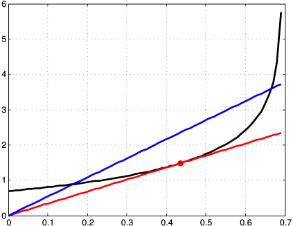
Figure 4: The graph of functions $y=h_{r}(t)$ (black), $y=(\alpha(r)-1)t$ (red) and $y=(\alpha-1)t$ for $\alpha>\alpha(r)$ (blue). The point $(t(r),h_{r}(t(r)))$ is marked by a red circle.

Let us define for $\alpha>1$

$$g(\alpha):=(\alpha-1)\ln(2(\alpha-1))-\alpha\ln(\alpha).$$ (55)

One can check that $g^{\prime\prime}(\alpha)>0$, and that $g^{\prime}(1+)=-\infty$ and $g(+\infty)=+\infty$. The graph of the function $\alpha\mapsto g(\alpha)$ is shown in Figure 5. For $r\geq 1$ we define $\alpha_{*}(r)$ to be the unique positive solution to the equation

$$g(\alpha)=\ln\left(\frac{1+r}{2}\right),\;\textnormal{or equivalently }\;\left[2\left(1-\frac{1}{\alpha}\right)\right]^{\alpha-1}=\frac{\alpha}{2}(r+1).$$ (56)

We can see $\alpha(1)$ (the solution to $g(\alpha)=0$) marked by a red circle on Figure 5.

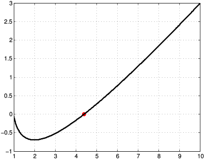
Figure 5: The graph of the function $\alpha\mapsto g(\alpha)$ defined in (55).

Let us show that $\alpha(r)$ satisfies equation (56) (i.e. that $\alpha(r)=\alpha_{*}(r)$. From the graph in Figure 4 it is clear that $\alpha(r)$ is characterized by the following system of two equations

$$h_{r}(t) = (\alpha-1)t,\qquad\qquad h_{r}^{\prime}(t)=\alpha-1.$$

This system expresses the fact that the graph of the straight line $y=(\alpha-1)t$ must be a tangent line to the curve $y=h_{r}(t)$ at the point of their intersection $t=t(r)$. From the equation $h_{r}^{\prime}(t)=\alpha-1$ we find that

$${\mathrm{e}}^{t}=2\left(1-\frac{1}{\alpha}\right)$$ (57)

and substituting this result into the first equation $h_{r}(t)=(\alpha-1)t$ (or into the equivalent equation (53)) we obtain (56).

Thus we have now proved that: (i) For $\alpha<\alpha(r)$ there do not exist equilibria of the form $((v)_{r},u,(v)_{r})$; (ii) For all $\alpha>\alpha(r)$ the equation (54) has two solutions, $0<t_{1}(\alpha)<t_{2}(\alpha)<\ln(2)$, such that $t_{1}(\alpha)$ is decreasing in $\alpha$ and $t_{2}(\alpha)$ is increasing in $\alpha$. These two solutions give us two equilibria of the form $((v)_{r},u,(v)_{r})$ (recall that $u=1/(2r+{\mathrm{e}}^{t})$).

Next, let us investigate stability of these equilibria. According to Lemma 3.18, the equilibrium is linearly stable if and only if

$$\frac{\alpha(uv)^{\alpha-1}}{2(r+1)(u^{\alpha}+rv^{\alpha})^{2}}<1,$$ (58)

and in the case $r=1$,

$$\frac{\alpha v^{\alpha-1}}{2(r+1)(u^{\alpha}+rv^{\alpha})}<1.$$ (59)

Applying the same ideas as in the proof of Lemmas 3.7 and 3.14 (taking the derivative $\partial/\partial\alpha$ of equation (54)) we check that the inequality (58) is equivalent to $\frac{\partial t}{\partial\alpha}>0$. One of the two equlibriums that we have found (the one corresponding to the solution $t_{1}(\alpha)$) is decreasing in $\alpha$, therefore it can not possibly be a stable equilibrium. At the same time the second solution $t_{2}(\alpha)$ is increasing in $\alpha$, therefore the condition (58) is satisfied. Let us look at the remaining condition (59). Using (51), we see that this is equivalent to

$$\left(\frac{u}{v}\right)^{\alpha-1}={\mathrm{e}}^{\scriptscriptstyle(\alpha-1)t_{2}}>\frac{\alpha}{2}.$$ (60)

Recall that we have denoted the unique solution to the equation $h_{r}(t)=(\alpha(r)-1)t$ by $t(r)$ (see Figure 4). Note that $\alpha>\alpha(r)$ and $t_{2}>t(r)$. Inequality (60) is satisfied when $\alpha=\alpha(r)$ and $t_{2}=t(r)$, since from formulas (56) and (57) it follows that

$${\mathrm{e}}^{\scriptscriptstyle(\alpha(r)-1)t(r)}=\left[2\left(1-\frac{1}{\alpha(r)}\right)\right]^{\alpha(r)-1}=\frac{\alpha(r)}{2}(r+1)>\frac{\alpha(r)}{2}.$$

If we increase $\alpha$ (while keeping $t_{2}=t(r)$ constant), then the inequality is still true, as the function on the left-hand side increases faster than the function on the right-hand side. Increasing $t_{2}$ will only increase the left-hand side, while keeping the right-hand side constant, and the required inequality is still true. Thus we have proved that the second equilibrium (the one with $v/u={\mathrm{e}}^{t_{2}(\alpha)}$) is linearly stable. ∎

3.5 Complete graph

Theorem 3.20.

Consider a complete graph on $n_{v}$ vertices and $n:=n_{v}(n_{v}-1)/2$ edges. For $n_{v}=3$, the equilibrium $\vec{1}/n$ is linearly stable if $\alpha<4/3$ (critical if equality holds), and it is linearly unstable if $\alpha>4/3$. For $n_{v}\geq 4$, the equilibrium $\vec{1}/n$ is linearly unstable.

Proof.

The case of $n_{v}=3$ (triangle graph) was considered in full detail in Theorem 3.8. Let us assume that $n_{v}\geq 4$. Let $K_{n_{v}}$ be the complete graph on $n_{v}$ vertices. We recall that the line-graph $L=L(K_{n_{v}})$ is defined by considering edges of $K_{n_{v}}$ as vertices of $L$, and the vertices of $L$ are adjacent if and only if the corresponding edges of $K_{n_{v}}$ are both incident to some vertex in $K_{n_{v}}$. The equations (16) give us

$$D_{i,j}(\vec{1}/n)=\begin{cases}-1+\alpha-\frac{\alpha}{n_{v}-1},\;\;\;&{\textnormal{ if }}\;i=j,\\ -\frac{\alpha}{2(n_{v}-1)},\;\;\;&{\textnormal{ if }}\;i\neq j,\text{ and }i,j\text{ are both incident to some vertex }x,\\ 0,\;\;\;&\text{ otherwise.}\end{cases}$$ (61)

Note that

$${\bf D}=\left(-1+\alpha-\alpha\frac{1}{n_{v}-1}\right){\bf I}-\frac{\alpha}{2(n_{v}-1)}{\bf A},$$ (62)

where ${\bf A}$ is the adjacency matrix of $L$. According to [5, Corollary 1.4.2], the matrix ${\bf A}$ has an eigenvalue $-2$ of degree $n-n_{v}$. This shows that the matrix ${\bf D}$ has an eigenvalue

$$-1+\alpha-\alpha\frac{1}{n_{v}-1}-\frac{\alpha}{2(n_{v}-1)}\times(-2)=-1+\alpha>0$$

of multiplicity $n-n_{v}$, and therefore $\vec{1}/n$ is a linearly unstable equilibrium. ∎

3.6 Circle graph

Lemma 3.21.

The equilibrium $\vec{v}=\vec{1}/n$ is linearly stable if and only if $n$ is odd and $\alpha<\cos\left(\tfrac{\pi}{2n}\right)^{-2}$.

Proof.

For the circle graph with $n$ vertices and edges, we label the edges $\{0,\dots,n-1\}$ around the circle (in the obvious way) and use addition and subtraction $\mod(n-1)$. Then, $\vec{v}$ is an equilibrium if and only if

$$v_{i}=\frac{1}{n}\frac{v_{i}^{\alpha}}{v_{i}^{\alpha}+v_{i+1}^{\alpha}}+\frac{1}{n}\frac{v_{i}^{\alpha}}{v_{i}^{\alpha}+v_{i-1}^{\alpha}}.$$ (63)

Moreover,

$$F(\vec{v})_{i}=-v_{i}+\frac{1}{n}\frac{v_{i}^{\alpha}}{v_{i}^{\alpha}+v_{i+1}^{\alpha}}+\frac{1}{n}\frac{v_{i}^{\alpha}}{v_{i}^{\alpha}+v_{i-1}^{\alpha}}$$

has derivatives

$$D_{i,i}(\vec{v})= -1+\frac{\alpha v_{i}^{\alpha-1}}{n}\left[\frac{1}{v_{i}^{\alpha}+v_{i+1}^{\alpha}}+\frac{1}{v_{i}^{\alpha}+v_{i-1}^{\alpha}}-\frac{v_{i}^{\alpha}}{(v_{i}^{\alpha}+v_{i+1}^{\alpha})^{2}}+\frac{v_{i}^{\alpha}}{(v_{i}^{\alpha}+v_{i-1}^{\alpha})^{2}}\right],$$

$$D_{i,i+1}(\vec{v})= -\frac{\alpha v_{i+1}^{\alpha-1}}{n}\frac{v_{i}^{\alpha}}{(v_{i}^{\alpha}+v_{i+1}^{\alpha})^{2}},$$

$$D_{i,i-1}(\vec{v})= -\frac{\alpha v_{i-1}^{\alpha-1}}{n}\frac{v_{i}^{\alpha}}{(v_{i}^{\alpha}+v_{i-1}^{\alpha})^{2}},$$

$$D_{i,k}(\vec{v})= ~{}0\quad\text{ otherwise.}$$

For $\vec{v}=\vec{1}/n$, these reduce to

$$D_{i,i}(\vec{1}/n)= -1+\frac{\alpha}{2},$$

$$D_{i,i+1}(\vec{1}/n)= D_{i,i-1}(\vec{1}/n)=-\frac{\alpha}{4},$$

$$D_{i,k}(\vec{1}/n)= ~{}0\quad\text{ otherwise.}$$

Thus, ${\bf D}$ is a circulant matrix with 3 consecutive $(\!\!\!\!\mod(n-1))$ non-zero entries $-\alpha/4$, $-1+\alpha/2$, $-\alpha/4$. Therefore its eigenvalues are of the form

$$\lambda_{j}= -1+\frac{\alpha}{2}-\frac{\alpha}{4}{\mathrm{e}}^{2\pi ij/n}-\frac{\alpha}{4}{\mathrm{e}}^{-2\pi ij/n}$$

$$= -1+\frac{\alpha}{2}-\frac{\alpha}{2}\cos(2\pi j/n),$$

for $j=0,\dots,n-1$. All of these eigenvalues are negative if and only if for every $j=0,\dots,n-1$,

$$\alpha[1-\cos(2\pi j/n)]<2.$$

When $n$ is even, the left hand side attains its maximum of $2\alpha$ at $j=n/2$ for which the stability criterion is $\alpha<1$. When $n$ is odd, the left hand side attains its maximum at $j=(n+1)/2$ for which the stability criterion becomes

$$\alpha<\frac{2}{1-\cos(\pi(1+1/n))}=\frac{2}{1+\cos(\pi/n)}=\frac{1}{\cos\left(\pi/2n\right)^{2}},$$

where the right hand side is greater than 1. ∎

Note that for $n=3$, this reduces to $\alpha<2/(1+1/2)=4/3$, which must be the case since for $n=3$ this corresponds to the case of fixed $m=2$, uniform $A_{t}$ (with $n=3$). By Theorem 1.22, for $n$ even, the vector $\vec{v}_{\text{alt}}=2(1,0,1,0,\dots,1,0)/n$ is a linearly-stable equilibrium for all $\alpha>1$.

4 Discussion and open problems

Regarding Conjecture 1.24.

We have shown that when $G$ is the triangle graph and $\alpha>4/3$, any stable equilibrium has some $v_{i}=0$. We believe that the same is true (for $\alpha>\alpha_{\scriptscriptstyle G}$) when $G$ is the line graph on 4 edges. Assuming that this can be verified, it is reasonable to expect that for any fixed $G$, and all $\alpha$ sufficiently large, the only linearly-stable equilibria are those admitted by whisker-forests.

We have shown that for all $\alpha>\alpha(r)$ there is a linearly-stable equilibrium (or a unique equilibrium that is critical) on a symmetric whisker-graph. We expect that the symmetry property is not needed. If this can be verified, it would imply that for any $G$, any whisker-forest admits a stable equilibrium for $\alpha$ sufficiently large. There are a great many problems about WARMs that remain open, among them are the following:

• Is it true that all $\vec{v}\in\mathcal{E}_{\alpha}$ for a WARM line graph with $3$ edges are symmetric (i.e., that $v_{1}=v_{3}$)?

• Can one prove non-convergence to linearly-unstable equilibria in our general setting?

• Is it in our general setting true that $\mathcal{A}\subset\mathcal{S}_{\alpha}$ when $\mathcal{S}_{\alpha}\neq\varnothing$?

More general models.

This work is inspired by modelling of the brain. We think of the signal entering, giving rise to our generalized Pólya urn. However, in the brain, signals are transmitted between several neurons, suggesting a model where signals perform a random motion (with or without branching of the signal). Without branching, this could be modelled using edge-reinforced random walks (see e.g., [8, 9, 21, 22, 16, 18] and the references therein) on graphs, killed at certain vertices. With branching, this would give rise to a certain kind of branching reinforced walk with killing. Such problems have attracted substantial attention oven the past decade.

Appendix A -    Proof of Theorem 1.14

The proof of Theorem 1.14 follows the proof of [3, Theorem 1.2] very closely. We repeat this argument almost exactly, only modifying the expression of the Lyapunov function and some related objects. We have included this material for the sake of completeness.

The main idea of the proof of Theorem 1.14 is to interpret the evolution of the WARM as a stochastic approximation algorithm (see [2]). We introduce several definitions and notations. We recall that $N_{t}^{\scriptscriptstyle(i)}$ denotes the number of balls of colour $i$ at time $t\in\mathbb{Z}^{+}$, $N_{0}^{\scriptscriptstyle(i)}=1$ and $n$ is the total number of colours. We assume that $p_{\varnothing}=0$, therefore the total number of balls at time $t$ is $n+t$. We denote $X_{t}^{\scriptscriptstyle(i)}:=N_{t}^{\scriptscriptstyle(i)}/(n+t)$ to be the proportion of balls of colour $i$. We define $C_{t}^{\scriptscriptstyle(i)}$ be the number of balls of colour $i$ which is added to the urn at time $t$, that is $C_{t}^{\scriptscriptstyle(i)}:=N_{t+1}^{\scriptscriptstyle(i)}-N_{t}^{\scriptscriptstyle(i)}$. We denote ${\mathcal{F}}_{t}:=\sigma\{\vec{N}_{u}\colon 1\leq u\leq t\}$. Note that $C_{t}^{\scriptscriptstyle(i)}\in\{0,1\}$ is a Bernoulli random variable, such that

$${\mathbb{P}}(C_{t}^{\scriptscriptstyle(i)}=1\mid{\mathcal{F}}_{t})=\sum\limits_{A\colon i\in A}p_{A}\frac{(X_{t}^{\scriptscriptstyle(i)})^{\alpha}}{\sum\limits_{j\in A}(X_{t}^{\scriptscriptstyle(j)})^{\alpha}},$$ (A.1)

moreover, we have $\sum_{i=1}^{n}C_{t}^{\scriptscriptstyle(i)}=1$ (since only one ball is added to the urn at time $t$). By definition, we have $N_{t+1}^{\scriptscriptstyle(i)}=N_{t}^{\scriptscriptstyle(i)}+C_{t}^{\scriptscriptstyle(i)}$, therefore

$$X_{t+1}^{\scriptscriptstyle(i)}-X_{t}^{\scriptscriptstyle(i)}=\frac{1}{n+t+1}\left(-X_{t}^{\scriptscriptstyle(i)}+C_{t}^{\scriptscriptstyle(i)}\right).$$ (A.2)

Denoting

$$F_{i}(x_{1},x_{2},\dots,x_{n}):=-x_{i}+\sum\limits_{A\colon i\in A}p_{A}\frac{x_{i}^{\alpha}}{\sum\limits_{j\in A}x_{j}^{\alpha}},$$

and using (A.1), we can rewrite (A.2) in the form

$$\vec{X}_{t+1}-\vec{X}_{t}=\gamma_{t}(F(\vec{X}_{t})+\vec{u}_{t}),$$ (A.3)

where $F=(F_{1},F_{2},\dots,F_{n})$, $\gamma_{t}:=1/(n+t+1)$ and $u_{t}^{\scriptscriptstyle(i)}:=C^{\scriptscriptstyle(i)}_{t}-{\mathbb{E}}[C^{\scriptscriptstyle(i)}_{t}\mid{\mathcal{F}}_{t}]$. Formula (A.3) expresses the WARM as a stochastic approximation algorithm. This is a classical approach to studying convergence of generalized Polya urns, as there exists a well-developed theory for stochastic approximation algorithms (see [2, 6, 11]). In particular, the result of Theorem 1.14, (ii) follows at once from (A.3) and [2, Proposition 7.5].

We write $A\sqsubset[n]$ when $A\subset[n]$ and $p_{A}>0$. Let us denote $c:=\tfrac{1}{2}\min\{p_{A}\colon A\sqsubset[n]\}$. We define $\Delta$ to be the set of $n$-tuples $(x_{1},x_{2},\dots,x_{n})\in\mathbb{R}^{n}$ such that

1. $x_{i}\geq 0$ and $\sum_{i=1}^{n}x_{i}=1$, and

2. for all $A\sqsubset[n]$ we have $\sum_{i\in A}x_{i}\geq c$.

Clearly $F:\Delta\mapsto T\Delta$ is Lipschitz. The following lemma is an analogue of [3, Lemma 3.4]:

Lemma A.1.

$\Delta$ is positively invariant under the ODE $\;\frac{{\textnormal{d}}\vec{v}(t)}{{\textnormal{d}}t}=F(\vec{v}(t))$.

Proof.

If $v$ belongs to the boundary of $\Delta$, then either $v_{i}=0$ for some $i\in[n]$, or there exists a set $A\sqsubset[n]$ with $\sum_{i\in A}v_{i}=c$. In the former case, since $F_{i}(\vec{v})=0$ if $v_{i}=0$, it is clear that $v(t)$ will stay on the corresponding boundary. Let us consider the latter case. Given a set $A$ with $p_{A}>0$, we have

$$\frac{{\textnormal{d}}}{{\textnormal{d}}t}\sum\limits_{i\in A}v_{i}=\sum\limits_{i\in A}\Big{(}-v_{i}+\sum\limits_{B\colon i\in B}p_{B}\frac{v_{i}^{\alpha}}{\sum\limits_{j\in B}v_{j}^{\alpha}}\Big{)}\geq\sum\limits_{i\in A}\Big{(}-v_{i}+p_{A}\frac{v_{i}^{\alpha}}{\sum\limits_{j\in A}v_{j}^{\alpha}}\Big{)}=-\sum\limits_{i\in A}v_{i}+p_{A}.$$

If $v$ is on the boundary of $\Delta$ and there exists a set $A$ such that $\sum_{i\in A}v_{i}=c$, then

$$\frac{{\textnormal{d}}}{{\textnormal{d}}t}\sum\limits_{i\in A}v_{i}\geq-\sum\limits_{i\in A}v_{i}+p_{A}=-c+p_{A}>0,$$

which means that $F$ points inward on the boundary of $\Delta$. ∎

We recall that ${\mathcal{E}}={\mathcal{E}}_{\alpha}$ denotes the set of equilibria of the WARM (the set of solutions to $F(\vec{v})=\vec{0}$).

Definition A.2 (Strict Lyapunov function).

A strict Lyapunov function for a vector field $F$ is a continuous map $L:\Delta\mapsto\mathbb{R}$ which is strictly monotone along any integral curve of $F$ outside of ${\mathcal{E}}$. In this case, we call $F$ gradient-like.

We define a function $L\colon\Delta\mapsto\mathbb{R}$ as

$$L(x_{1},x_{2},\dots,x_{n})=-\sum\limits_{i=1}^{n}x_{i}+\frac{1}{\alpha}\sum\limits_{A}p_{A}\ln\Big{(}\sum\limits_{j\in A}x_{j}^{\alpha}\Big{)}.$$ (A.4)

One can check that

$$x_{i}\frac{\partial L}{\partial x_{i}}=-x_{i}+\sum\limits_{A:i\in A}p_{A}\frac{x_{i}^{\alpha}}{\sum\limits_{j\in A}x_{j}^{\alpha}}=F_{i}(\vec{x})$$ (A.5)

The following result is an analogue of [3, Lemma 4.1]:

Lemma A.3.

$L$ is a strict Lyapunov function for $F$.

Proof.

Assume that $v(t)=(v_{1}(t),v_{2}(t),\dots,v_{n}(t))$ is an integral curve of $F$, which means that $\frac{{\textnormal{d}}v}{{\textnormal{d}}t}=F(v)$, then

$$\frac{{\textnormal{d}}}{{\textnormal{d}}t}L(v(t))=\sum\limits_{i=1}^{n}\frac{\partial L}{\partial x_{i}}\frac{{\textnormal{d}}v_{i}}{{\textnormal{d}}t}=\sum\limits_{i=1}^{n}v_{i}\left(\frac{\partial L}{\partial x_{i}}\right)^{2}\geq 0.$$

The last expression is zero if and only if $v_{i}\left(\frac{\partial L}{\partial x_{i}}\right)^{2}=0$ for all $i\in[n]$, which is equivalent to $F(v)=0$ (or $v\in{\mathcal{E}}$).

∎

The proof of Theorem 1.14(i) relies on the following result (see [1], [2] and [3, Theorem 3.3]):

Theorem A.4.

Let $F\colon\mathbb{R}^{n}\mapsto\mathbb{R}^{n}$ be a continuous gradient-like vector field with unique integral curves, let ${\mathcal{E}}$ be its equilibria set, let $L$ be a strict Lyapunov function, and let $\vec{X}_{t}$ be a solution to the recursion (A.3), where $(\gamma_{t})_{t\geq 0}$ is a decreasing sequence and $(\vec{u}_{t})_{t\geq 0}\subset\mathbb{R}^{n}$. Assume that

• $({\vec{X}}_{t})_{t\geq 0}$ is bounded,

• for each $T>0$,

  $$\lim\limits_{t\to+\infty}\Big{(}\sup\limits_{\{k\colon 0\leq\tau_{k}-\tau_{n}\leq T\}}\Big{\|}\sum\limits_{i=n}^{k-1}\gamma_{i}\vec{u}_{i}\Big{\|}\Big{)}=0,$$

  where $\tau_{n}=\sum\limits_{i=0}^{n-1}\gamma_{i}$, and

• $L({\mathcal{E}})\subset\mathbb{R}$ has empty interior.

Then the limit set of $(\vec{X}_{t})_{t\geq 0}$ is a connected subset of ${\mathcal{E}}$.

Proof of Theorem 1.14(i). Again, the proof follows the proof of [3, Theorem 1.2] very closely. Note that $\gamma_{t}=1/(n+t+1)$ satisfies

$$\lim\limits_{t\to+\infty}\gamma_{t}=0,\qquad{\textnormal{ and }}\qquad\sum\limits_{t\geq 0}\gamma_{t}=+\infty.$$

It is obvious from the definition that $(\vec{X}_{t})_{t\geq 0}$ is bounded, thus condition (i) of Theorem A.4 is satisfied. Let us verify condition (ii). We define

$$\vec{M}_{t}:=\sum\limits_{s=0}^{t}\gamma_{s}\vec{u}_{s}.$$

It is clear that $(\vec{M}_{t})_{t\geq 0}$ is a martingale adapted to the filtration $({\mathcal{F}}_{t})_{t\geq 0}$. Furthermore, since for any $t\geq 0$,

$$\sum\limits_{s=0}^{t}{\mathbb{E}}\left[\|\vec{M}_{s+1}-\vec{M}_{s}\|^{2}|{\mathcal{F}}_{s}\right]\leq\sum\limits_{s=0}^{t}\gamma_{s+1}^{2}\leq\sum\limits_{s=0}^{\infty}\gamma_{s}^{2}<\infty,$$

the sequence $(\vec{M}_{t})_{t\geq 0}$ converges almost surely and in $L^{2}$ to a finite random vector. In particular, it is a Cauchy sequence and therefore, the condition (ii) holds almost surely.

Now we need to verify condition (iii) in Theorem A.4. We need to distinguish between equilibria lying in the interior of ${\mathcal{E}}$ and those lying on the boundary. For each subset $S\subset[n]$, we define

$$\Delta_{S}:=\{v\in\Delta\colon v_{i}=0{\textnormal{ iff }}i\notin S\}.$$

We see that $\Delta_{S}$ is a face of $\Delta$, it is also a manifold with corners, and, extending the result of Lemma A.1, it is easy to see that $\Delta_{S}$ is positively invariant under the ODE $\frac{{\textnormal{d}}\vec{v}}{{\textnormal{d}}t}=F(\vec{v})$.

Definition A.5.

$\vec{v}\in\Delta_{S}$ is an $S$-singularity for $L$ if

$$\frac{\partial L}{\partial v_{i}}(\vec{v})=0\;{\textnormal{ for all }}i\in S.$$

Let ${\mathcal{E}}_{\scriptscriptstyle S}\subset\Delta_{S}$ denote the set of $S$-singularities for $L$.

Lemma A.6.

${\mathcal{E}}=\cup_{S\subset[n]}{\mathcal{E}}_{\scriptscriptstyle S}$.

Proof.

$\vec{v}\in{\mathcal{E}}$ means that $F(\vec{v})=0$, and due to (A.5) this is equivalent to $v_{i}\frac{\partial L}{\partial v_{i}}=0$. Therefore, $\vec{v}\in{\mathcal{E}}$ implies that for all $i\in[n]$, either $v_{i}=0$ or $\frac{\partial L}{\partial v_{i}}=0$. ∎

In order to check condition (iii) of Theorem A.4, we need to show that $L({\mathcal{E}})=0$. For any $S\subset[n]$, the function $L$ restricted to $\Delta_{S}$ is a $C^{\infty}$ function, thus by Sard’s theorem $L({\mathcal{E}}_{\scriptscriptstyle S})$ has zero Lebesgue measure, which implies that $L({\mathcal{E}})$ has zero Lebesgue measure, which in turn implies that $L({\mathcal{E}})$ has empty interior. This verifies condition (iii) in Theorem A.4, and ends the proof of Theorem 1.14(i). ∎

References

- [1] Benaïm, M. A dynamical system approach to stochastic approximations. SIAM J. Control Optim. 34 (1996), no. 2, 437-472.
- [2] Benaïm, M. Dynamics of stochastic approximation algorithms. Séminaire de probabilités (Strasbourg), tome 33 (1999), p. 1-68.
- [3] Benaïm, M., Benjamini, I., and Chen, J., and Lima, Y. A generalised Pólya’s urn with graph-based interactions. Random Structures and Algorithms (to appear).
- [4] Benaïm, M., Raimond, O., and Schapira, B. Strongly reinforced vertex-reinforced-random-walk on the complete graph. Preprint, 2012.
- [5] Brouwer, A.E. and Haemers, W.H. Spectra of graphs. Springer, New York, 2012.
- [6] Chen, H.-F. Stochastic Approximation and Its Applications. Nonconvex Optimization and Its Applications, Vol. 64, Springer, 2002.
- [7] Chung, F., Handjani, S., and Jungreis, D. Generalizations of Pólya’s urn problem, Annals of Combinatorics, 7:141–153, 2003.
- [8] Davis, B. Reinforced random walk. Probab. Theory Related Fields 84(2):203–229, 1990.
- [9] Durrett, R, Kesten, H., and Limic, V. Once edge-reinforced random walk on a tree. Probab. Theory Related Fields, 122(4):567–592, 2002.
- [10] Holmes, M., and Kuznetsov, A. Exponentially reinforced Pólya urns with graph-based competition. In preparation.
- [11] Kushner, H. J., and Yin, G. G. Stochastic approximation and recursive algorithms and applications. Applications of Mathematics, vol. 35, second edition, Springer, 2003.
- [12] Launay, M. Urnes Interagissantes. PhD thesis, Université Aix-Marseille, 2012.
- [13] Launay, M. Interacting Urn Models. http://arxiv.org/abs/1101.1410, 2012.
- [14] Launay, M. Urns with simultaneous drawing. http://arxiv.org/abs/1201.3495, 2012.
- [15] Launay, M., and Limic, V. Generalized Interacting Urn Models. http://arxiv.org/abs/1207.5635, 2012.
- [16] Limic, V. and Tarrès, P. Attracting edge and strongly edge reinforced walks. Ann. Probab., 35(5):1783–1806, 2007.
- [17] Mahmoud, H.M. Pólya Urn Models CRC Press, Boca Raton FL, 2009).
- [18] Merkl, F. and Rolles, S. Recurrence of edge-reinforced random walk on a two-dimensional graph. Ann. Probab., 37(5):1679–1714, 2009.
- [19] Moler, J. A., Plo, F., and San Miguel, M., Almost sure convergence of urn models in a random environment, In Proceedings of the Seminar on Stability Problems for Stochastic Models, Part I (Eger, 2001), J. Math. Sci. (New York), 111:3566–3571, 2002.
- [20] Oliveira, R., and Spencer, J. Connectivity transitions in networks with super-linear preferential attachment Internet Math. 2:121–163, 2005.
- [21] Pemantle, R. Phase transition in reinforced random walk and RWRE on trees. Ann. Probab., 16(3):1229–1241, 1988.
- [22] Pemantle, R. A survey of random processes with reinforcement, Probab. Surv.4: 1–79, 2007.
- [23] Nishino, T. Function theory in several complex variables. Translations of Mathematical Monographs, Vol. 193, American Mathematical Society, 2001.
- [24] Shabat, B.V. Introduction to Complex Analysis: part II, functions of several variables. Translations of Mathematical Monographs, Vol. 110, American Mathematical Society, 1992.