Baltic Astronomy, vol. 23, 37–54, 2014

HOW DOES THE STRUCTURE OF SPHERICAL DARK MATTER HALOES AFFECT THE TYPES OF ORBITS IN DISK GALAXIES?

Euaggelos E. Zotos

  Department of Physics, School of Science, Aristotle University of Thessaloniki,
GR-541 24, Thessaloniki, Greece; e-mail: evzotos@physics.auth.gr

Received: 2014 March 24; accepted: 2014 March 30

Abstract.  The main objective of this work is to determine the character of orbits of stars moving in the meridional $(R,z)$ plane of an axially symmetric time-independent disk galaxy model with a central massive nucleus and an additional spherical dark matter halo component. In particular, we try to reveal the influence of the scale length of the dark matter halo on the different families of orbits of stars, by monitoring how the percentage of chaotic orbits, as well as the percentages of orbits of the main regular resonant families evolve when this parameter varies. The smaller alignment index (SALI) was computed by numerically integrating the equations of motion as well as the variational equations to extensive samples of orbits in order to distinguish safely between ordered and chaotic motion. In addition, a method based on the concept of spectral dynamics that utilizes the Fourier transform of the time series of each coordinate is used to identify the various families of regular orbits and also to recognize the secondary resonances that bifurcate from them. Our numerical computations reveal that when the dark matter halo is highly concentrated, that is when the scale length has low values the vast majority of star orbits move in regular orbits, while on the oth er hand in less concentrated dark matter haloes the percentage of chaos increases significantly. We also compared our results with early related work.

Key words:  galaxies: kinematics and dynamics, structure; chaos; dark matter haloes

1.   INTRODUCTION

A large amount of observational data indicate that disk galaxies are often surrounded by massive and extended dark matter haloes. Undoubtedly the best tool to study dark matter haloes in galaxies is the galactic rotation curve derived from neutral hydrogen HI (e.g., Clemens 1985; Persic & Salucci 1995; Honma & Sofue 1997). The determination of the exact shape of a dark matter halo however, is a challenging task. Numerical simulations suggest that dark matter haloes are not only spherical, but may also be prolate, oblate, or even triaxial (e.g., Merritt & Fridman 1996; Cooray 2000; Kunihito et al. 2000; Olling & Merrifield 2000; Jing & Suto 2002; Wechsler et al. 2002; Kasun & Evrard 2005; Allgood et al. 2006; Capuzzo-Dolcetta et al. 2007; Wang et al. 2009; Evans & Bridle 2009). The variety of the shapes of galactic haloes points out that the structure of these objects plays an important role in the orbital behavior and, generally, in the dynamics of a galaxy.

The presence of dark matter haloes in galaxies is indeed expected by the standard cold dark matter (CDM) cosmology models regarding formation of galaxies. The most well-known model for CDM haloes is the flattened cuspy Navarro Frenk White (NFW) model (Navarro et al. 1996, 1997), which is simplified to be spherical. Most CDM models, however, take considerable deviations from the standard spherically symmetric dark matter halo distributions into account. For instance, the model of formation of dark matter haloes in a universe dominated by CDM by Frenk et al. (1988) produced triaxial haloes with a preference for prolate configurations. In addition, numerical simulations of dark matter halo formation conducted by Dubinski & Carlberg (1991) are consistent with haloes that are triaxial and flat. There are roughly equal numbers of dark haloes with oblate and prolate forms.

Over the last years several dynamical models have been developed in order to model the properties of dark matter haloes. A three-dimensional model consisting of a disk, a spherical nucleus, and a logarithmic asymmetric dark matter halo component was used in Caranicolas & Zotos (2009). For simplicity, a nearly spherical dark matter halo with an internal, small deviation from spherical symmetry described by the term $-\lambda x^{3}$ was chosen. The results of this work suggest that even small asymmetries in the galactic halo play a significant role in the nature of three-dimensional orbits, mainly by depopulating the box family; the box orbits become chaotic as the value of the internal perturbation increases. In the same vein, a similar three-dimensional composite galaxy model was utilized in Caranicolas & Zotos (2011), however, in this case the dark mater halo was modeled by a mass Plummer potential. The mass of the halo was found to be an important physical quantity, acting as a chaos controller in galaxies. In particular, the percentage of chaotic orbits reduces rapidly as the mass of the spherical dark halo increases. Moreover, it was found that the amount of chaos is higher in asymmetric triaxial galaxies when they are surrounded by less concentrated spherical dark halo components.

Furthermore, in two earlier papers (Caranicolas 1997; Papadopoulos & Caranicolas 2006) two-dimensional, axially symmetric or non-axially symmetric active galaxy models with an additional spherical halo component were studied. In both cases it was observed that the presence of a spherical halo resulted in reduced area in the phase space occupied by the chaotic orbits. Moreover, the behavior of orbits in an active galaxy with a biaxial (prolate or oblate) dark matter halo was investigated recently in Caranicolas & Zotos (2010). In this work, we studied how the regular or chaotic nature of orbits is influenced by some important quantities of the system, such as the flattening parameter of the halo, the scale length of the halo component, and the conserved component of the angular momentum. It was found that when a biaxial halo component is present there is a linear relationship between the chaotic percentage in the phase plane and the flattening parameter. In contrast, the relation between chaos and the scale length of the halo was found to be not linear but exponential. A similar model was used in Helmi (2004) for numerical simulations of the evolution of a system like the Sagittarius dSph in a variety of galactic potentials varying the flattening parameter.

In a very recent paper Zotos (2014) we revealed how all the dynamical parameters of a multi component model influence the percentages of orbits. For the description of the properties of the dark matter halo we used a softened logarithmic potential. Usually , logarithmic potentials are utilized for modeling dark matter haloes, however, in the present work we decided to use a mass type potential. We made this choice for two main reasons: (i) we wanted to know the exact amount of mass of the halo; logarithmic potentials cannot give this information and (ii) it would be of particular interest to compare the corresponding results derived using two different types of model potentials for the dark matter halo.

The layout of the paper is as follows: Section 2 contains a detailed presentation of the structure and the properties of our galactic gravitational model. In Section 3 we describe the computational methods we used in order to determine the character and the classification of orbits. In the following section, we investigate how the scale length of the dark matter halo influences the nature as well as the evolution of the percentages of the different families of orbits. The paper ends with Section 5, where the main conclusions of our numerical analysis and the discussion are presented.

2.   PROPERTIES OF THE GALACTIC MODEL

In this investigation we try to reveal the regular or chaotic nature of orbits of stars moving in the meridional plane of an axially symmetric disk galaxy with a central massive nucleus and a spherical dark matter halo. We use the usual cylindrical coordinates $(R,\phi,z)$, where $z$ is the axis of symmetry.

The total gravitational potential $\Phi(R,z)$ in our model consists of three components: the central nuclear component $\Phi_{\rm n}$, the disk potential $\Phi_{\rm d}$ and the spherical dark matter halo component $\Phi_{\rm h}$. For the description of the central nucleus, we use a Plummer potential (e.g., Binney & Tremaine 2008)

$$\Phi_{\rm n}(R,z)=\frac{-GM_{\rm n}}{\sqrt{R^{2}+z^{2}+c_{\rm n}^{2}}}.$$ (1)

Here $G$ is the gravitational constant, while $M_{\rm n}$ and $c_{\rm n}$ are the mass and the scale length of the nucleus, respectively. This potential has been used successfully in the past to model and, therefore, interpret the effects of the central mass component in a galaxy (see e.g., Hasan & Norman 1990; Hasan et al. 1993; Zotos 2011b, 2012; Zotos & Carpintero 2013; Zotos 2014). At this point, we must emphasize that we do not include any relativistic effects, because the nucleus represents a bulge rather than a black hole or any other compact object.

On the other hand, the galactic disk is represented by the well-known Miyamoto-Nagai potential Miyamoto & Nagai (1975)

$$\Phi_{\rm d}(R,z)=\frac{-GM_{\rm d}}{\sqrt{R^{2}+\left(\alpha+\sqrt{h^{2}+z^{2}}\right)^{2}}},$$ (2)

where, $M_{\rm d}$ is the mass of the disk, $\alpha$ is the scale length of the disk, and $h$ corresponds to the disk’s scale height (e.g., Zotos 2011a). Furthermore, the dark matter halo is modeled by another Plummer potential

$$\Phi_{\rm h}(R,z)=\frac{-GM_{\rm h}}{\sqrt{R^{2}+z^{2}+c_{\rm h}^{2}}},$$ (3)

where $M_{\rm h}$ and $c_{\rm h}$ are the mass and the scale length of the dark halo, respectively.

We use a system of galactic units where the unit of length is 1 kpc, the unit of velocity is 10 km s^-1, and $G=1$. Thus, the unit of mass is $2.325\times 10^{7}{\rm M}_{\odot}$, that of time is $0.9778\times 10^{8}$ yr, the unit of angular momentum (per unit mass) is 10 km kpc^-1 s^-1, and the unit of energy (per unit mass) is 100 km²s^-2. In these units, the values of the involved parameters are: $M_{\rm n}=400$ (corresponding to $9.3\times 10^{9}$ M_⊙), $c_{\rm n}=0.25$, $M_{\rm d}=7000$ (corresponding to $1.63\times 10^{11}$ M${}_{\odot})$, $\alpha=3$, $h=0.175$ and $M_{\rm h}=10000$ (corresponding to $2.325\times 10^{11}$ M_⊙). The particular values of the parameters were chosen with a Milky Way-type galaxy in mind (e.g., Allen & Santillán 1991). The above-mentioned set of values of the parameters, which are kept constant throughout the numerical calculations, secures positive mass density everywhere and is free of singularities. The scale length of the dark matter halo, on the other hand, is treated as a parameter.

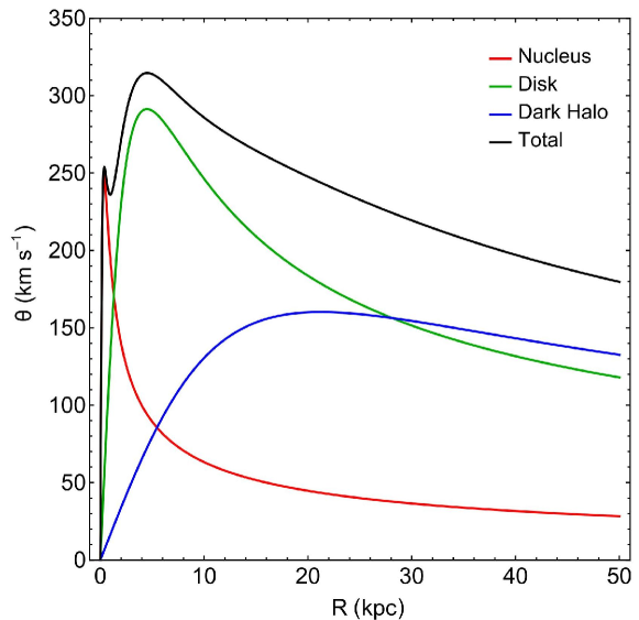
Figure 1: A plot of the rotation curve in our galactic model. We distinguish the total circular velocity (black) and also the contributions from the central massive nucleus (red), the disk (green) and that of the dark matter halo (blue).

Undoubtedly, one of the most important physical quantities in galaxies is the circular velocity in the galactic plane $(z=0)$ (e.g., Zotos, 2011c) which is defined as,

$$\theta(R)=\sqrt{R\left|\frac{\partial\Phi(R,z)}{\partial R}\right|_{z=0}}.$$ (4)

In Fig. 1 we present a plot of $\theta(R)$ (black curve) for our galactic model when $c_{\rm h}=15$. Moreover, in the same plot, the red line shows the contribution from the central nucleus, the green curve is the contribution from the disk, while the blue line corresponds to the contribution form the dark matter halo. It is seen that each contribution prevails in different distances form the galactic center. In particular, at small distances, when $R\leq 2$ kpc, the contribution from the massive central nucleus dominates, while at mediocre distances, $2<R<28$ kpc, the disk contribution is the dominant factor. On the other hand, at very large galactocentric distances, $R>28$ kpc, we see that the contribution from the dark matter halo prevails, thus forcing the rotation curve to remain flat with increasing distance from the center. We also observe the characteristic local minimum (at $R\simeq 2$ kpc) of the rotation curve due to the massive nucleus, which appears when fitting the observed data to a galactic model (e.g., Gómez et al. 2010; Irrgang et al. 2013).

Exploiting the fact that the $L_{z}$-component of the total angular momentum $L_{z}$ is conserved because the gravitational potential $\Phi(R,z)$ is axisymmetric, orbits can be described by means of the effective potential

$$\Phi_{\rm eff}(R,z)=\Phi(R,z)+\frac{L_{z}^{2}}{2R^{2}}.$$ (5)

Then, the basic equations of motion on the meridional plane are

$$\ddot{R}=-\frac{\partial\Phi_{\rm eff}}{\partial R},\ \ \ \ddot{z}=-\frac{\partial\Phi_{\rm eff}}{\partial z},$$ (6)

while the equations governing the evolution of a deviation vector ${\bf{w}}=(\delta R,\delta z,\delta\dot{R},\delta\dot{z})$, which joins the corresponding phase space points of two initially nearby orbits, needed for the calculation of the standard indicators of chaos (the SALI in our case), are given by the variational equations

$$\dot{(\delta R)} = \delta\dot{R},\ \ \ \dot{(\delta z)}=\delta\dot{z},$$

$$(\dot{\delta\dot{R}}) = -\frac{\partial^{2}\Phi_{\rm eff}}{\partial R^{2}}\delta R-\frac{\partial^{2}\Phi_{\rm eff}}{\partial R\partial z}\delta z,$$

$$(\dot{\delta\dot{z}}) = -\frac{\partial^{2}\Phi_{\rm eff}}{\partial z\partial R}\delta R-\frac{\partial^{2}\Phi_{\rm eff}}{\partial z^{2}}\delta z.$$ (7)

Consequently, the corresponding Hamiltonian to the effective potential given in Eq. (5) can be written as

$$H=\frac{1}{2}\left(\dot{R}^{2}+\dot{z}^{2}\right)+\Phi_{\rm eff}(R,z)=E,$$ (8)

where $\dot{R}$ and $\dot{z}$ are momenta per unit mass, conjugate to $R$ and $z$ respectively, while $E$ is the numerical value of the Hamiltonian, which is conserved. Therefore, an orbit is restricted to the area in the meridional plane satisfying $E\ geq\Phi_{\rm eff}$.

3.   COMPUTATIONAL METHODS

In our numerical exploration, we seek to determine whether an orbit is regular or chaotic. Several indicators of chaos are available in the literature; we chose the SALI indicator introduced in Skokos (2001). The time-evolution of SALI strongly depends on the nature of the computed orbit since when the orbit is regular the SALI exhibits small fluctuations around nonzero values, while on the other hand, in the case of chaotic orbits the SALI after a small transient period it tends exponentially to zero approaching the limit of the accuracy of the computer $(10^{-16})$. Therefore, the particular time-evolution of the SALI allows us to distinguish fast and safely between regular and chaotic motion. The time-evolution of a regular (R) and a chaotic (C) orbit for a time period of $10^{4}$ time units is presented in Fig. 2 We observe, that both regular and chaotic orbits exhibit the expected behavior. Nevertheless, we have to define a specific numerical threshold value for determining the transition from regularity to chaos. After conducting extensive numerical experiments, integrating many sets of orbits, we conclude that a safe threshold value for the SALI taking into account the total integration time of $10^{4}$ time units is the value $10^{-7}$. The horizontal, blue and dashed line in Fig. 2 corresponds to that threshold value which separates regular from chaotic motion. In order to decide whether an orbit is regular or chaotic, one may use the usual method according to which we check after a certain and predefined time interval of numerical integration, if the value of SALI has become less than the established threshold value. Therefore, if SALI $\leq 10^{-7}$ the orbit is chaotic, while if SALI $>10^{-7}$ the orbit is regular.

However, depending on the particular location of each orbit, this threshold value can be reached more or less quickly, as there are phenomena that can hold off the final classification of an orbit (i.e., there are special orbits called “sticky” orbits, which behave regularly for long time periods before they finally drift away from the regular regions and start to wander in the chaotic domain, revealing their true chaotic nature fully. A characteristic example of a sticky orbit (S) in our galactic model can be seen in Fig. 2, where we observe that the chaotic character of the particular sticky orbit is revealed only after a vast integration time of about 3000 time units.

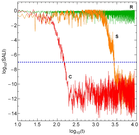
Figure 2: Time-evolution of the SALI of a regular orbit (green color – R), a sticky orbit (orange color – S) and a chaotic orbit (red color – C) in our model for a time period of $10^{4}$ time units. The horizontal, blue dashed line corresponds to the threshold value $10^{-7}$ which separates regular from chaotic motion. The chaotic orbit needs only about 150 time units in order to cross the threshold, while the sticky orbit requires about 3000 time units so as to reveal its true chaotic nature.

To examine the orbital properties (chaoticity or regularity) of the dynamical system, we need to establish some samples of initial conditions of orbits. The best approach, undoubtedly, would have been to extract these samples of orbits from the distribution function of the model. Unfortunately, this is not available, so we followed another course of action. To determine the character of the orbits in our model, we chose, for each value of the scale length $c_{h}$ of the dark matter halo, a dense grid of initial conditions regularly distributed in the area allowed by the value of the orbital energy $E$. Our investigation takes place in the phase space $(R,\dot{R})$ for a better understanding of the orbital structure of the system. The step separation of the initial conditions along the $R$ and $\dot{R}$ axes (in other words the density of the grids) was controlled in such a way that always there are at least 50 000 orbits to be integrated. The grids of initial conditions of orbits whose properties will be examined are defined as follows: we consider orbits with the initial conditions $(R_{0},\dot{R_{0}})$ with $z_{0}=0$, while the initial value of $\dot{z_{0}}$ is obtained from the energy integral (8). For each initial condition, we numerically integrated the equations of motion (6) as well as the variational equations (7) with a double precision Bulirsch-Stoer algorithm (e.g., Press et al. 1992) with a small time step of the order of $10^{-2}$, which is sufficient enough for the desired accuracy of our computations (i.e., our results practically do not change by halving the time step). In all cases, the energy integral (Eq. 8) was conserved better than one part in $10^{-10}$, although for most orbits it was better than one part in $10^{-11}$.

Each orbit was numerically integrated for a time interval of $10^{4}$ time units ($10^{12}$ yr), which corresponds to a time span of the order of hundreds of orbital periods. The particular choice of the total integration time is an element of great importance, especially in the case of the sticky orbits. A sticky orbit could be easily misclassified as regular by any chaos indicator, if the total integration interval is too small, so that the orbit does not have enough time to reveal its true chaotic character. Thus, all the initial conditions of the orbits of a given grid were integrated, as we already said, for $10^{4}$ time units, thus avoiding sticky orbits with a stickiness at least of the order of $10^{2}$ Hubble time. All the sticky orbits that do not show any signs of chaoticity for $10^{4}$ time units are counted as regular orbits since such vast sticky periods are completely out of the scope of our research.

A first step toward the understanding of the overall behavior of our system is knowing whether the orbits in the galactic model are regular or chaotic. Also of particular interest is the distribution of regular orbits into different families. Therefore, once the orbits have been characterized as regular or chaotic, we then further classify the regular orbits into different families by using a frequency analysis method (Carpintero & Aguilar 1998; Muzzio et al. 2005). Initially, Binney & Spergel (1982, 1984) proposed a technique, dubbed spectral dynamics, for this particular purpose. Later on, this method has been extended and improved by Carpintero & Aguilar (1998) and Šidlichovský and Nesvorný (1996). In a recent work, Zotos & Carpintero (2013) the algorithm was refined even further so it can be used to classify orbits in the meridional plane. In general terms, this method computes the Fourier transform of the coordinates of an orbit, identifies its peaks, extracts the corresponding frequencies, and searches for the fundamental frequencies and their possible resonances. Thus, we can easily identify various families of regular orbits and also recognize the secondary resonances that bifurcate from them. This technique has been applied in several previous papers (e.g., Zotos & Carpintero 2013; Caranicolas & Zotos 2013; Zotos & Caranicolas 2013, 2014) in the field of orbit classification (not only regular versus chaotic, but also separating regular orbits into different regular families) in different galactic gravitational potentials.

Before closing this section, we would like to make a clarification about the nomenclature of orbits. All the orbits of an axisymmetric potential are in fact three-dimensional (3D) loop orbits, i.e., orbits that always rotate around the axis of symmetry in the same direction. However, in dealing with the meridional plane, the rotational motion is lost, so the path that the orbit follows onto this plane can take any shape, depending on the nature of the orbit. Following the same approach of the previous papers of this series, we characterize an orbit according to its behavior in the meridional plane. If, for example, an orbit is a rosette lying in the equatorial plane of the axisymmetric potential, it will be a linear orbit in the meridional plane, a tube orbit will be a 2:1 orbit, etc. We should emphasize that we use the term “box orbit” for an orbit that conserves circulation, but this refers only to the circulation provided by the meridional plane itself. Because of the their boxlike shape in the meridional plane, such orbits were originally called “boxes” (e.g., Ollongren 1962), even though their three-dimensional shapes are more similar to doughnuts (see the review of Merritt 1999). Nevertheless, we kept this formalism to maintain continuity with all the previous papers of this series.

4.   ORBIT CLASSIFICATION

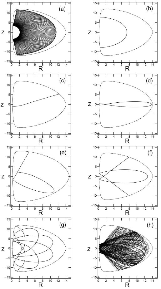
Figure 3: Orbit collection of the basic types of orbits in our galaxy model: (a) box orbit; (b) 2:1 banana-type orbit; (c) 1:1 linear orbit; (d) 2:3 fish-type orbit; (e) 3:2 boxlet orbit; (f) 4:3 boxlet orbit; (g) 10:7 boxlet orbit, one of our “orbits with higher resonance”; (h) chaotic orbit. $R$ and $z$ are the cylindrical coordinates.

Table 1: Types and initial conditions of the orbits shown in Fig. 3 (a-h). In all cases, $z_{0}=0$, $\dot{z_{0}}$ is found from the energy integral, Eq. (8), while $T_{\rm per}$ is the period of the resonant parent periodic orbits.

Figure	Type	$R_{0}$	$\dot{R_{0}}$	$T_{\rm per}$
Fig. 3a	box	2.10000000	0.00000000	–
Fig. 3b	2:1 banana	7.39378964	0.00000000	1.90395532
Fig. 3c	1:1 linear	3.39916301	42.85969675	1.28112540
Fig. 3d	2:3 boxlet	13.75776855	0.00000000	2.55010488
Fig. 3e	3:2 boxlet	0.85335785	20.81656490	3.94317967
Fig. 3f	4:3 boxlet	12.74460663	0.00000000	5.12001897
Fig. 3g	10:7 boxlet	2.48051157	0.00000000	12.99471468
Fig. 3h	chaotic	0.25000000	0.00000000	–

In this section, we will numerically integrate several sets of orbits, in an attempt to distinguish the regular or chaotic nature of motion of stars. We use the sets of initial conditions described in the previous section to construct the respective grids, always adopting values inside the zero velocity curve (ZVC). In all cases, the energy was set equal to $-1000$, the angular momentum of the orbits is $L_{\rm z}=10$, while the scale length of the dark halo is treated as a parameter. Here, we have to point out that the energy level controls the size of the grid and particularly the $R_{\rm max}$ which is the maximum possible value of the $R$ coordinate. We chose that energy level $(E=-1000)$ which yields 10 kpc $<R_{\rm max}<17$ kpc. To study how scale length of the dark halo $c_{\rm h}$ influences the level of chaos, we let it vary while fixing all other parameters of our galaxy model. As already noted, we fix the values of all other parameters and integrate orbits in the meridional plane for the set $c_{\rm h}=\{5,7.5,10,...,30\}$. Once the values of the parameters were chosen, we computed a set of initial conditions as described in Section 3 and integrated the corresponding orbits computing the SALI of the orbits and then classifying regular orbits into different families.

Our numerical investigation reveals that in our galaxy model there are eight basic types of orbits: (i) chaotic orbits; (ii) box orbits; (iii) 1:1 linear orbits; (iv) 2:1 banana-type orbits; (v) 2:3 fish-type orbits; (vi) 3:2 resonant orbits; (vii) 4:3 resonant orbits and (viii) orbits with other resonances (i.e., all resonant orbits not included in the former categories). It turns out that for these last orbits the corresponding percentage is less than 1% in all cases, and therefore their contribution to the overall orbital structure of the galaxy is insignificant. A $n:m$ resonant orbit would be represented by $m$ distinct islands of invariant curves in the phase plane $(R,\dot{R})$ and $n$ distinct islands of invariant curves in the $(z,\dot{z})$ surface of section. In Fig. 3 (a-h) we present examples of each of the basic types of regular orbits, plus an example of a chaotic one. In all cases, we set $c_{\rm h}=15$ (except for the 3:2 resonant orbit, where $c_{\rm h}=12.5$). The orbits shown in Figs. 3a and 3h were computed until $t=200$ time units, while all the parent periodic orbits were computed until one period has completed. The black thick curve circumscribing each orbit is the limiting curve in the meridional plane $(R,z)$ defined as $\Phi_{\rm eff}(R,z)=E$. Table 1 shows the types and the initial conditions for each of the depicted orbits; for the resonant cases, the initial conditions and the period $T_{\rm per}$ correspond to the parent periodic orbits.

At this point, we should note that the 1:1 resonance is usually the hallmark of the loop orbits and both coordinates oscillate with the same frequency in their main motion. Their mother orbit is a closed loop orbit. Moreover, when the oscillations are in phase, the 1:1 orbit degenerates into a linear orbit (the same as in Lissajous figures made with two oscillators). In our meridional plane, however, 1:1 orbits do not have the shape of a loop. In fact, their mother orbit is linear (e.g., Fig. 3c) , and thus they do not have a hollow (in the meridional plane), but fill a region around the linear mother, always oscillating along the $R$ and $z$ directions with the same frequency. We designate these orbits “1:1 linear open orbits” to differentiate them from true meridional plane loop orbits, which have a hollow and also always rotate in the same direction.

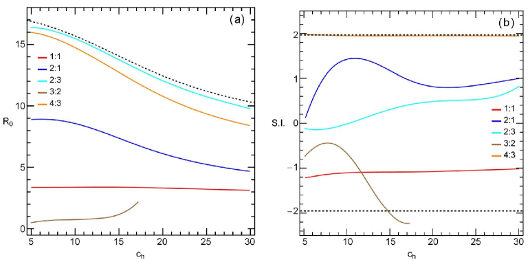
Figure 4: Panel (a), left: the $(R_{0},c_{\rm h})$ characteristic curves of the orbital families; panel (b), right: evolution of the stability index S.I. of the families of periodic orbits shown in panel (a). The black horizontal dashed lines at –2 and +2 delimit the range of S.I. for which the periodic orbits are stable.

In Fig. 4a we present a very informative diagram the so-called “characteristic” orbital diagram Contopoulos & Mertzanides (1977). It shows the evolution of the $R$ coordinate of the initial conditions of the parent periodic orbits of each orbital family as a function of the variable scale length of the dark halo $c_{\rm h}$. Here we should emphasize, that for orbits starting perpendicular to the $R$-axis, we need only the initial condition of $R_{0}$ in order to locate them on the characteristic diagram. On the other hand, for orbits not starting perpendicular to the $R$-axis (i.e, the 1:1 and 3:2 resonant orbits) initial conditions as position-velocity pairs $(R,\dot{R})$ are required and, therefore, the characteristic diagram is three-dimensional providing full information regarding the interrelations of the initial conditions in a tree of families of periodic orbits. The outermost black dashed line denotes the permissible area of motion as it is defined by the particular value of the energy; the region above this line is forbidden. Furthermore, the diagram shown in Fig. 4b is called the “stability diagram” (Contopoulos & Barbanis 1985; Contopoulos & Magnenat 1985), and it illustrates the stability of all the families of periodic orbits in our dynamical system when the numerical value of $c_{\rm h}$ varies, while all other parameters remain constant. A periodic orbit is stable if only the stability index (S.I.) (Meyer & Hall 1992; Zotos 2013) is between –2 and +2. This diagram help us to monitor the evolution of S.I. of the resonant periodic orbits as well as the transitions from stability to instability and vice versa. Our computations suggest that almost all resonant families are stable throughout the interval $c_{\rm h}\in[5,30]$. We observe that the curve of the 4:3 is located very close to the upper stability limit, evolving asymptotically, but in never crosses the critical value (+2), at least inside the studied interval of values of $c_{\rm h}$. Contrary, the 3:2 family is stable only for $c_{\rm h}<14.71$, while for larger values of the dark halo scale length the resonant periodic orbits become unstable and eventually the 3:2 family terminates when $c_{\rm h}=17.1923$.

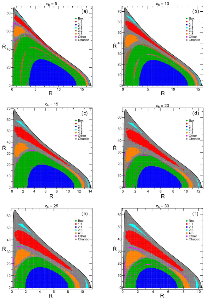
Figure 5: Orbital structure of the phase plane $(R,\dot{R})$ of our galaxy model for different values of the scale length of the dark halo $c_{\rm h}$.

In Figs. 5 (a–f) we present six grids of initial conditions $(R_{0},\dot{R_{0}})$ of orbits that we have classified for different values of the scale length of the dark matter halo $c_{\rm h}$. These color-coded grids of initial conditions are equivalent to the classical Poincaré surfaces of section (PSS) and allow us to determine what types of orbits occupy specific areas in the phase plane $(R,\dot{R})$. The outermost black thick curve is the limiting curve which is defined as

$$\frac{1}{2}\dot{R}^{2}+\Phi_{\rm eff}(R,0)=E.$$ (9)

In Fig. 5a we see that when the spherical dark matter halo is very concentrated $(c_{\rm h}=5)$, the vast majority of the phase plane is covered by initial conditions corresponding to regular orbits, while chaos is confined only at the outer parts of the phase plane thus displaying a thin chaotic layer. In particular, we can distinguish the seven main types of regular orbits presented earlier: (i) 2:1 banana-type orbits located at the central region of the grid; (ii) box orbits situated mainly outside of the 2:1 resonant orbits; (iii) 1:1 open linear orbits form the elongated island of initial conditions; (iv) 2:3 fish-type resonant orbits form the set of three small islands at the outer parts of the grid; (v) 3:2 resonant orbits producing several stability islands inside the box region; (vi) 4:3 resonant orbits form the chain of three islands; and (vii) other types of resonances producing extremely small islands embedded both in the chaotic and box areas. However, as the value of scale length increases and the dark matter halo becomes less and less concentrated, we observe that the amount of box and 2:1 resonant orbits reduces thus giving place to other resonant orbits (i.e., the 1:1, 2:3 and 4:3 families) to grow, while at the same time the chaotic region increases in size. When $c_{\rm h}=15$, Fig. 5c shows that there is no indication whatsoever of the 3:2 family. This is expected because for $14.71<c_{\rm h}<17.1923$ the 3:2 resonant orbits are unstable (see Fig. 4, a-b). This means that the periodic point of the 3:2 resonance is indeed present in Fig. 5c, although evidently deeply buried in the box area. For relatively large values of the scale length $(c\geq 20)$ one may see in Figs. 5 (d–f) that there is a substantial chaotic region, while higher resonant orbits (i.e., the 4:5, 6:5, 7:5 and 10:7) produce thin filaments of initial conditions inside the box an chaotic regions. It should also be mentioned that the permissible area on the phase plane (both the $R_{\rm max}$ and the radial velocity $\dot{R}$ of the stars near the center of the galaxy are reduced) is reduced with increasing scale length of the dark matter halo.

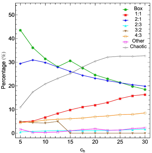
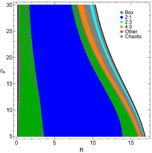
Figure 6: Evolution of the percentages of different types of orbits in the phase plane $(R,\dot{R})$ of our galaxy model, when varying the value of the scale length of the dark halo $c_{\rm h}$.

Figure 7: Orbital structure of the $(R,c_{\rm h})$ plane. This diagram gives a detailed analysis of the evolution of orbits starting perpendicularly to the $R$-axis when the value of the halo scale length varies in the interval $c_{\rm h}\in[5,30]$.

The following Fig. 7 shows the evolution of the percentages of the chaotic and all types of regular orbits as a function of the scale length of the dark matter halo, $c_{\rm h}$. One may observe that, as we proceed to higher values of the scale length, the percentage of chaotic orbits increases, while at the same time, the rate of box and 2:1 resonant orbits reduces steadily. In the case of very low scale length $(c_{\rm h}=5)$ almost the entire phase plane is covered only by initial conditions of regular orbits; about 45% of the phase plane corresponds to initial conditions of box orbits and only about 10% of it to chaotic orbits. However, when $c_{\rm h}>17.5$, chaotic orbits is the most populated family dominating the phase plane. It is also seen that, when $c_{\rm h}>22.5$, the percentage of chaotic orbits seem to saturate around 32%. At the highest studied value of the scale length $(c_{\rm h}=30)$ or in other words when the dark halo is very loose, the rates of box, 2:1 and 1:1 resonant orbits tend to a common value (around 20%), thus sharing three fifths of the phase plane. Furthermore, our numerical analysis suggests that the percentages of the 1:1, 2:3 and 4:3 families grow with increasing scale length, although following different rates. In fact, the amount of 1:1 resonant orbits increases almost linearly, while the 2:3 and 4:3 families exhibit a less sharp increase, so we may argue that these types of orbits are practically immune to the change of $c_{\rm h}$. Moreover, for $c_{\rm h}<12.5$, the 3:2 family holds a constant rate around 5%, while for larger values of $c_{\rm h}$ it vanishes. In addition, we may say that in general terms, all other resonant families possess throughout very low percentages (always less than 5%) so, varying the value of $c_{\rm h}$ only shuffles the orbital content among them. Thus, taking into account all the above-mentioned analysis, we may conclude that in the phase plane $(R,\dot{R})$ the types of orbits, that are mostly influenced by the scale length of the spherical dark matter halo, are the box, 1:1, 2:1 and the chaotic orbits.

The grids in the phase plane $(R,\dot{R})$ can provide information on the phase space mixing for only a fixed value of the halo scale length $c_{\rm h}$. However, Hénon back in the 60s considered a plane which provides information about regions of regularity and regions of chaos using the section $z=\dot{R}=0$, $\dot{z}>0$, i.e., the test particles (stars) are launched on the $R$-axis, parallel to the $z$-axis and in the positive $z$-direction. Thus, in contrast to the previously discussed grids, only orbits with pericenters on the $R$-axis are included and therefore the value of $c_{\rm h}$ is now used as an ordinate. Fig. 7 shows the orbital structure of the $(R,c_{\rm h})$-plane when $c_{\rm h}\in[5,30]$. In order to be able to monitor with sufficient accuracy and details the evolution of the families of orbits, we defined a dense grid of $10^{5}$ initial conditions in the $(R,c_{\rm h})$-plane. It is evident, that the vast majority of the grid is covered either by box or 2:1 resonant orbits, while initial conditions of chaotic orbits are mainly confined to right outer part of the $(R,c_{\rm h})$-plane. Furthermore, the 2:3 and 4:3 resonances produce thin stability layers. It is also seen, that several families of higher resonant orbits are present, corresponding to thin filaments of initial conditions living inside the box region. It should be emphasized, that the maximum value of the $R$ coordinate $(R_{\rm max})$ is reduced with increasing $c_{\rm h}$. We must also stress out that the $(R,c_{\rm h})$-plane contains only such orbits starting perpendicularly to the $R$-axis, while orbits whose initial conditions are pairs of position-velocity (i.e., the 1:1 and 3:2 resonant families) are obviously not included.

5.   DISCUSSION AND CONCLUSIONS

The aim of the present work was to investigate how influential is the scale length of the dark matter halo on the level of chaos and on the distribution of regular families among its orbits. For this purpose, we used an analytic, axially symmetric galactic gravitational model which embraces the general features of a disk galaxy with a dense, massive, central nucleus and an additional spherical dark matter halo component. To simplify our study, we chose to work in the meridional plane $(R,z)$, thus reducing three-dimensional to two-dimensional motion. We kept the values of all other parameters constant, because our main objective was to determine the influence of the scale length on the percentages of the orbits. Our thorough and detailed numerical analysis suggests that the level of chaos as well as the distribution in regular families is indeed very dependent on the halo scale length.

Undoubtedly, a disk galaxy with a central massive nucleus and a dark matter halo is a very complex entity and therefore, we need to assume some necessary simplifications and assumptions in order to be able to study mathematically the orbital behavior of such a complicated stellar system. For this purpose, our total gravitational model is intentionally simple and contrived, in order to give us the ability to study all different aspects regarding the kinematics and dynamics of the model. Nevertheless, contrived models can surely provide an insight into more realistic stellar systems, which unfortunately are very difficult to be explored, if we take into account all the astrophysical aspects (i.e., gas, spirals, mergers, etc.). On the other hand, self-consistent models are mainly used when conducting $N$-body simulations. However, this application is entirely out of the scope of the present paper. Once more we have to point out that the simplicity of our model is necessary, otherwise it would be extremely difficult, or even impossible, to apply the extensive and detailed numerical calculations presented in this study. Similar gravitational models with the same limitations and assumptions were used successfully several times in the past in order to investigate the orbital structure in much more complicated galactic systems.

Our numerical investigation takes place in the phase space $(R,\dot{R})$ for a better understanding the orbital structure of the system. Since a distribution function of our galaxy model was not available for extracting the different samples of orbits, we had to follow an alternative path. Thus, for determining the regular or chaotic character of orbits in our models, we defined dense grids of initial conditions regularly distributed in the area allowed by the value of the total orbital energy $E$, in the phase space. To show how the halo scale length influences the orbital structure of the system, for each case we presented color-coded grids of initial conditions, which allow us to visualize what types of orbits occupy specific areas in the phase space. Each orbit was integrated numerically for a time period of $10^{4}$ time units ($10^{12}$ yr), which corresponds to a time span of the order of hundreds of orbital periods. The particular, choice of the total integration time was made in order to eliminate sticky orbits (classifying them correctly as chaotic orbits) with a stickiness at least of 100 Hubble times. Then, we made a step further in an attempt to distribute all regular orbits into different families. Therefore, once an orbit has been characterized as regular applying the SALI method, we then further classified it using a frequency analysis method. This method calculates the Fourier transform of the coordinates and velocities of an orbit, identifies its peaks, extracts the corresponding frequencies and then searches for the fundamental frequencies and their possible resonances.

The main outcomes of our research can be summarized as follows:

$\bullet$ Several types of regular orbits were found to exist in our galactic gravitational model, while there are also extended chaotic domains separating the areas of regularity. In particular, a large variety of resonant orbits (i.e., 1:1, 2:1, 2:3, 3:2, 4:3 and higher resonant orbits) are present, thus making the orbital structure more rich. Here we must clarify that by the term “higher resonant orbits” we refer to resonant orbits with a rational quotient of frequencies made from integers $>$ 5, which of course do not belong to the main families.

$\bullet$ It was found that in the phase space $(R,\dot{R})$ the scale length of the dark matter halo influences mainly box, 1:1, 2:1 and chaotic orbits. Moreover, the majority of stars move in regular orbits and in general terms, box and 2:1 resonant orbits are the most populated family of regular orbits throughout the range of values of $c_{\rm h}$. All resonant families are stable apart from the 3:2 family which consists of a mixture of stable and unstable resonant orbits.

$\bullet$ The largest amount of chaos, about 32%, was measured for high values of the scale length $(c_{\rm h}>22.5)$ corresponding to very loose dark matter haloes, while as $c_{\rm h}$ decreases and the dark halo becomes more and more concentrated, the amount of chaotic orbits is reduced rapidly, and for the low enough values of the scale length, $(c_{\rm h}<7)$, about 90% of the tested orbits were found to be regular.

The influence of the scale length of the dark halo on the character of orbits has been an active field of investigation over the years. In Caranicolas & Zotos (2011) the dark mater halo was also modeled by a mass Plummer type potential and it was observed that the amount of chaos in triaxial galaxies is higher when they are surrounded by less concentrated dark matter haloes. This behavior is in absolute agreement with the current results. A logarithmic potential has been used in Zotos (2014) to describe the properties of a biaxial dark matter halo. There it was found that in galaxy models with prolate or oblate dark matter haloes, the scale length of the halo affects mostly box, 2:1 banana-type, resonant and chaotic orbits, while a similar relation between the amount of chaos an the scale length was obtained. Therefore we may conclude that the scale length, which is the parameter controlling how concentrated is the dark matter halo, has roughly the same impact on the character of orbits in galaxies regardless the particular type of the potential used for modeling the dark matter halo.

References

- Allen & Santillán (1991) Allen C., Santillán A. 1991, RevMexAA, 22, 255
- Allgood et al. (2006) Allgood B., Flores R. A., Primack J. R. et al. 2006, MNRAS, 367, 1781
- Binney & Spergel (1982) Binney J., Spergel D. 1982, ApJ, 252, 308
- Binney & Spergel (1984) Binney J., Spergel D. 1984, MNRAS, 206, 159
- Binney & Tremaine (2008) Binney J. Tremaine S. 2008, Galactic Dynamics, Princeton Univ. Press
- Capuzzo-Dolcetta et al. (2007) Capuzzo-Dolcetta R., Leccese L., Merritt D., Vicari A. 2007, ApJ, 666, 165
- Caranicolas (1997) Caranicolas N. D. 1997, Ap&SS, 246, 15
- Caranicolas & Zotos (2009) Caranicolas N. D., Zotos E. E. 2009, Baltic Astronomy, 18, 205
- Caranicolas & Zotos (2010) Caranicolas N. D., Zotos E. E. 2010, AN, 331, 330
- Caranicolas & Zotos (2011) Caranicolas N. D., Zotos E. E. 2011, RAA, 11, 811
- Caranicolas & Zotos (2013) Caranicolas N. D., Zotos E. E. 2013, PASA, 30, 49
- Carpintero & Aguilar (1998) Carpintero D. D., Aguilar L. A. 1998, MNRAS, 298, 1
- Clemens (1985) Clemens D. P. 1985, ApJ, 295, 422
- Contopoulos & Barbanis (1985) Contopoulos G., Barbanis B. 1985, A&A, 153, 44
- Contopoulos & Magnenat (1985) Contopoulos G., Magnenat P. 1985, CeMec, 37, 387
- Contopoulos & Mertzanides (1977) Contopoulos G., Mertzanides C. 1977, A&A, 61, 477
- Cooray (2000) Cooray A. R. 2000, MNRAS, 313, 783
- Dubinski & Carlberg (1991) Dubinski J., Carlberg R. G. 1991, ApJ, 378, 496
- Evans & Bridle (2009) Evans A. K. D., Bridle S. 2009, ApJ, 695, 1446
- Frenk et al. (1988) Frenk C. S., White S. D. M., Davis M., Efstathiou G. 1988, ApJ, 327, 507
- Gómez et al. (2010) Gómez F., Helmi A., Brown A.G.A., Li Y.S. 2010, MNRAS, 408, 935
- Hasan & Norman (1990) Hasan H., Norman C.A. 1990, ApJ, 361, 69
- Hasan et al. (1993) Hasan H., Pfenniger D., Norman C.A. 1993, ApJ, 409, 91
- Helmi (2004) Helmi A. 2004, PASA, 21, 212
- Honma & Sofue (1997) Honma M., Sofue Y. 1997, PASJ, 49, 453
- Irrgang et al. (2013) Irrgang A., Wilcox B., Tucker E., Schiefelbein L. 2013, A&A, 549, A137
- Jing & Suto (2002) Jing Y.P., Suto Y. 2002, ApJ, 574, 538
- Kasun & Evrard (2005) Kasun S.F., Evrard A.E. 2005, ApJ, 629, 781
- Kunihito et al. (2000) Kunihito I., Takahiro T., Takashi N. 2000, ApJ, 528, 51
- Merritt (1999) Merritt D. 1999, PASP, 111, 129
- Merritt & Fridman (1996) Merritt D., Fridman T. 1996, ApJ, 460, 136
- Meyer & Hall (1992) Meyer K.R., Hall G.R., 1992, Introduction to Hamiltonian Dynamical Systems and the N-Body Problem, Springer-Verlag
- Miyamoto & Nagai (1975) Miyamoto W., Nagai R. 1975, PASJ, 27, 533
- Muzzio et al. (2005) Muzzio J.C., Carpintero D.D., Wachlin F.C. 2005, CeMDA, 91, 173
- Navarro et al. (1996) Navarro J.F., Frenk C.S., White S.D.M. 1996, ApJ, 462, 563
- Navarro et al. (1997) Navarro J.F., Frenk C.S., White S.D.M. 1997, ApJ, 490, 493
- Olling & Merrifield (2000) Olling R.P., Merrifield M.R. 2000, MNRAS, 311, 361
- Ollongren (1962) Ollongren A. 1962, Bulletin of the Astronomical Institutes of the Netherlands, 16, 241
- Papadopoulos & Caranicolas (2006) Papadopoulos N.J., Caranicolas N.D. 2006, New Astronomy, 12, 11
- Persic & Salucci (1995) Persic M., Salucci P. 1995, ApJS, 99, 501
- Press et al. (1992) Press H.P., Teukolsky S.A, Vetterling W.T., Flannery B.P. 1992, Numerical Recipes in FORTRAN 77, 2nd Ed., Cambridge Univ. Press, Cambridge, USA
- Šidlichovský and Nesvorný (1996) Šidlichovský M., Nesvorný D. 1996, CeMDA, 65, 137
- Wang et al. (2009) Wang H., Mo H.J., Jing Y.P., Guo Y., van den Bosch F.C., Yang X. 2009, MNRAS, 394, 398
- Wechsler et al. (2002) Wechsler R.H., Bullock J.S., Primack J.R., Kravtsov A.V., Dekel A. 2002, ApJ, 568, 52
- Skokos (2001) Skokos C. 2001, J. Phys. A Math. Gen., 34, 10029
- Zotos (2011a) Zotos E.E. 2011a, Baltic Astronomy, 20, 77
- Zotos (2011b) Zotos E.E. 2011b, Baltic Astronomy, 20, 339
- Zotos (2011c) Zotos E.E. 2011c, New Astronomy, 16, 391
- Zotos (2012) Zotos E.E. 2012, New Astronomy, 17, 576
- Zotos (2013) Zotos E.E. 2013, Nonlinear Dynamics, 73, 931
- Zotos (2014) Zotos E.E. 2014, A&A, 563, A19
- Zotos & Carpintero (2013) Zotos E.E., Carpintero D.D. 2013, CeMDA, 116, 417
- Zotos & Caranicolas (2013) Zotos E.E., Caranicolas N.D. 2013, A&A, 560, A110
- Zotos & Caranicolas (2014) Zotos E.E., Caranicolas N.D. 2014, Nonlinear Dynamics, 76, 323