Global dynamics and inflationary center manifold and slow-roll approximants

Abstract

We consider the familiar problem of a minimally coupled scalar field with quadratic potential in flat Friedmann-Lemaître-Robertson-Walker cosmology to illustrate a number of techniques and tools, which can be applied to a wide range of scalar field potentials and problems in e.g. modified gravity. We present a global and regular dynamical systems description that yields a global understanding of the solution space, including asymptotic features. We introduce dynamical systems techniques such as center manifold expansions and use Padé approximants to obtain improved approximations for the ‘attractor solution’ at early times. We also show that future asymptotic behavior is associated with a limit cycle, which shows that manifest self-similarity is asymptotically broken toward the future, and give approximate expressions for this behavior. We then combine these results to obtain global approximations for the attractor solution, which, e.g., might be used in the context of global measures. In addition we elucidate the connection between slow-roll based approximations and the attractor solution, and compare these approximations with the center manifold based approximants.

PACS numbers: 04.20.-q, 98.80.-k, 98.80.Bp, 98.80.Jk

1 Introduction

The present paper is part of a research program that uses global dynamical systems methods to study spatially homogeneous cosmological models and cosmological perturbations for a wide variety of sources and gravity theories. The overall purpose of this program is: (i) To produce regularized global dynamical systems in order to obtain a global picture of the solution space of various cosmological models, thus determining the possible and likely cosmological consequences of different physical assumptions. (ii) To describe the asymptotic features of the models. (iii) To introduce and assess different approximation schemes that approximately describe solutions in their asymptotic regimes, and to combine them to give the entire solutions approximatively, in global dynamical systems settings.

To achieve the above goals require the introduction of various more or less sophisticated mathematical techniques in an area that to a large extent is dominated by heuristic arguments and local considerations. This is the price to be payed in order to achieve clarified rigor and to obtain a global understanding of cosmological possibilities that contextualize various heuristic results when they are essentially correct, and to sometimes reveal that some heuristic beliefs are actually unfounded myths that rather reflect hopes than what is actually the case.

In the present paper we consider a scalar field that is minimally coupled to the Einstein equations in flat Friedmann-Lemaître-Robertson-Walker (FLRW) cosmology with a quadratic potential. This is a simple and thoroughly studied problem and this is precisely why we choose it; the main purpose with the present paper is to present new ideas and methods in the setting of this familiar problem which are subsequently to be used (and sometimes modified) in a series of forthcoming papers that address increasingly complicated and therefore less understood problems. Moreover, some of the results for the current model turn out to reflect some rather general features, valid for much more general problems. It should, however, be pointed out that discussions about the recent results of BICEP2 [1] (see e.g. [2, 3] as examples of recent reactions to BICEP2) also motivate taking a renewed look at the classic problem of a minimally coupled scalar field with a quadratic potential.

The present scalar field problem has a quite long history. For brevity we only give the key historical references that serve as the starting point for the present work, namely the papers by Belinskiǐ et al. [4, 5, 6, 7], Rendall [8, 9], and Liddle et al. [10]. (A few other examples of references that describe minimally coupled scalar field cosmology in dynamical systems settings are [11, 12, 13], with additional references therein.)

The first goal of this paper is to present a global dynamical systems picture of the solution space, which furthermore gives a clear picture of the various past and future asymptotic states. This naturally brings the so-called attractor solution into focus in a global dynamical systems setting.

The second goal is to determine possible asymptotic behavior at early and late times. In particular we establish that late time behavior is associated with a particular type of asymptotic self-similarity breaking. At early times we show that the generic asymptotes are given by a massless scalar field state while a special type of de Sitter state describes the asymptotic behavior of the so-called attractor solution.

The third goal is to introduce, describe and assess a variety of approximation techniques that all boil down to giving an approximation for the attractor solution. In particular, we will show that the familiar slow-roll approximation and its slow-roll expansion extensions is just such an approximation scheme for the attractor solution at early times. This suggests that one should explicitly take the past asymptotic behavior of the attractor solution as the starting point for an approximation scheme. The attractor solution turns out to originate from a non-hyperbolic fixed point, which can be treated by means of center manifold theory to yield an expansion that gives an approximation for the attractor solution. In addition we show how so-called Padé (or, more generally, Canterbury) approximants can be used to analytically improve the range and rate of convergence for the various approximation expansions.

The fourth goal is to combine the center manifold based Padé approximants and the approximate solutions for the non-self-similar behavior at late times to obtain global approximations for the attractor solution.

The outline of the paper is as follows. In the next section we first present a regular unconstrained 2-dimensional dynamical system on a compact state space for a scalar field with a quadratic potential that is minimally coupled to the Einstein equations in flat FLRW cosmology. We then perform a global dynamical systems analysis identifying future and past behavior, and it is shown that the so-called attractor solution corresponds to a 1-dimensional unstable center submanifold of a certain non-hyperbolic fixed point. In particular we derive series expansions and improve their convergence properties and range by using Padé approximants. We also give approximations for the behavior at late times and use this together with the center manifold results to provide a global analytical approximate description of the attractor solution. In Section 3 we extend the slow-roll approximant results of Liddle et al. [10] to higher orders, and show how they provide approximations for the attractor solution in the present global dynamical systems context. These results, in combination with numerics, are then compared with the center manifold results to assess the accuracy and range of the various types of approximations. In Section 4 we further discuss our results and their implications for more general potentials and models.

2 Dynamical systems approach

The Einstein and scalar field equations for a minimally coupled scalar field $\phi(t)$ with potential $V(\phi)=\frac{1}{2}m^{2}\phi^{2}$ for flat FLRW cosmology are given by

$$3H^{2} ={\textstyle{1\over 2}}\dot{\phi}^{2}+{\textstyle{1\over 2}}m^{2}\phi^{2},$$ (1a)

$$\dot{H} =-{\textstyle{1\over 2}}\dot{\phi}^{2},$$ (1b)

$$0 =\ddot{\phi}+3H\dot{\phi}+m^{2}\phi,$$ (1c)

where an overdot signifies the derivative with respect to synchronous time, $t$. Throughout we use (reduced Planck) units such that $c=1=8\pi G$, where $c$ is the speed of light and $G$ is the gravitational constant. (In the inflationary literature the gravitational constant $G$ is often replaced by the Planck mass, $G=1/m_{\mathrm{Pl}}^{2}$.) In addition, $H$ is the Hubble variable, which is given by $H=\dot{a}/a$, where $a(t)$ is the cosmological scale factor, and throughout we assume an expanding Universe, i.e. $H>0$. The deceleration parameter $q$ is defined via $\dot{H}=-(1+q)H^{2}$, and due to (1b) it is therefore given by

$$q=-1+\frac{1}{2}\left(\frac{\dot{\phi}}{H}\right)^{2}.$$ (2)

It is also of interest to define the effective equation of state parameter $w_{\phi}$:

$$w_{\phi}:=\frac{p_{\phi}}{\rho_{\phi}}=\frac{{\textstyle{1\over 2}}\dot{\phi}^{2}-{\textstyle{1\over 2}}m^{2}\phi^{2}}{{\textstyle{1\over 2}}\dot{\phi}^{2}+{\textstyle{1\over 2}}m^{2}\phi^{2}},$$ (3)

and hence $q=\frac{1}{2}(1+3w_{\phi})$, a relation that holds for an arbitrary potential in flat FLRW cosmology.

Heuristically $3H^{2}$ in eq. (1a) can be viewed as an energy which according to eq. (1b) is decreasing. Furthermore, eq. (1c) can be interpreted as describing a nonlinearly damped harmonic oscillator, where $3H\dot{\phi}$ is the friction term, which suggests that the scalar field $\phi$ oscillates with decreasing amplitude toward the future and that $(H,\dot{\phi},V(\phi),\phi)\rightarrow(0,0,0,0)$, which is indeed the case. However, in these variables $q$ in eq. (2) becomes ill-defined, and the above heuristic picture says nothing about what happens with this important physical observable.

Moreover, reversing the time direction leads to a heuristic picture of a harmonic oscillator that gains energy, but in the past limit where $H\rightarrow\infty$ the energy driving term $3H\dot{\phi}$ becomes ill-defined and again the heuristic picture breaks down. One might take the viewpoint that the limit $H\rightarrow\infty$ is irrelevant since it would take one beyond the Planck regime where the classical description fails, but this would be a mistake. As we will see, an understanding of the classical limit $H\rightarrow\infty$ is necessary in order to understand the situation for large $H$, where the classical picture is expected to hold.

Furthermore, these heuristic considerations only yield rough qualitative pictures, which in addition say little about the asymptotic regimes. To obtain quantitative results, and to obtain results that yield a global dynamical picture, illustrating the entire solution space and its properties, requires a reformulation of the field equations that regularize them on a bounded state space that includes the limits $H\rightarrow\infty$ and $H\rightarrow 0$.

2.1 Global dynamical systems formulation

To obtain a global dynamical system on a relatively compact state space, which can be regularly extended to include its boundary, we define

$$T :=\frac{m}{m+H},$$ (4a)

$$\theta :=\arctan\left(\frac{\dot{\phi}}{m\phi}\right),$$ (4b)

and a new independent variable $\bar{\tau}$,

$$\frac{d\bar{\tau}}{dt}:=m+H,$$ (5)

which leads to the dynamical system

$$\frac{dT}{d\bar{\tau}} =3T(1-T)^{2}\sin^{2}\theta=\frac{3}{2}T(1-T)^{2}(1-\cos 2\theta),$$ (6a)

$$\frac{d\theta}{d\bar{\tau}} =-T-\frac{3}{2}(1-T)\sin 2\theta.$$ (6b)

The physical relatively compact state space ${\bf S}$ is defined by a finite cylinder with $T=0$ and $T=1$ as invariant boundary subsets, which can be included to yield the state space $\bar{\bf S}$. The interpretation in terms of a cylinder is perhaps most easily seen by introducing $T$ and the two variables

$$\Sigma_{\dagger}=\frac{\dot{\phi}}{\sqrt{6}H}\quad\text{and}\quad X=\frac{m\phi}{\sqrt{6}H}.$$ (7)

Together with the time choice $\bar{\tau}$, this leads to a 3-dimensional dynamical system for $T,\Sigma_{\dagger},X$ obeying the constraint (1a), which takes the form

$$1=\Sigma_{\dagger}^{2}+X^{2},$$ (8)

and thus $T,\Sigma_{\dagger}$ and $X$ describe a cylinder with unit radius. Solving the constraint (8) globally by introducing $\theta$ via

$$\Sigma_{\dagger}=\sin\theta,\quad X=\cos\theta$$ (9)

yields the present dynamical systems formulation. Note that the system (6) admits a discrete symmetry since it is invariant under the transformation $\theta\rightarrow\theta+\pi$, which is a reflection of that $V(\phi)$ is invariant under $\phi\rightarrow-\phi$.

In terms of the new variables the Hubble variable $H$, the scalar field $\phi$, and $\dot{\phi}$, are given by

$$\frac{H}{m} =\frac{1-T}{T},$$ (10a)

$$\phi =\sqrt{6}\left(\frac{1-T}{T}\right)\cos\theta,$$ (10b)

$$\dot{\phi} =\sqrt{6}m\left(\frac{1-T}{T}\right)\sin\theta,$$ (10c)

and hence constant $T$ surfaces in the state space ${\bf S}$ correspond to constant values of $H$. The deceleration parameter $q$ and the effective equation of state parameter $w_{\phi}$ are given by

$$q =-1+3\sin^{2}\theta={\textstyle{1\over 2}}(1-3\cos 2\theta),$$ (11a)

$$w_{\phi} =2\sin^{2}\theta-1=-\cos 2\theta.$$ (11b)

As a consequence a solution is accelerating as long as $\sin^{2}\theta<\frac{1}{3}$ (for future use in figures, note that $\arcsin(1/\sqrt{3})\approx\frac{\pi}{5}$).

Note that the present variables are the same as those used by Rendall in [8], where $T$ was denoted by $u$ and $\bar{\tau}$ by $\tau$, although the present state space was never used for global purposes in that paper. In addition, $T$ and $\theta$ are closely related to the variables $\rho,\theta,\psi$ used in e.g. [6], where $\theta=\pi/4$ in the flat FLRW case while $\psi$ corresponds to the present $\theta$. However, that work used different projections to describe the dynamics. In our opinion the presently used state space description has the advantage of clearly giving a global description of the dynamics, including at past and future asymptotic times.

Finally, it should also be pointed out that the system (6) is a reduced system. The equation for the scale factor $a$ has been decoupled. This equation is obtained from $H=\dot{a}/a$, where the above changes of independent and dependent variables yield

$$\frac{da}{d\bar{\tau}}=(1-T)a,$$ (12)

which leads to a quadrature for $a$ once the system (6) has been solved. If one furthermore wants to express things in terms of the synchronous proper time variable $t$, one needs to integrate the relation $mdt=T(\bar{\tau})d\bar{\tau}$, which follows from eqs. (5) and (10a).

2.2 Dynamical system for early times

Although the system (6) gives an illustrative global picture of the solution space, it might not yield the best variables for describing non-global state space structures. Below we are going to be interested in approximating the attractor solutions at early times. In this case we obtain a simpler system, which results in a more convenient analysis, by introducing the variables

$$\tilde{T} :=\frac{m}{H},$$ (13a)

$$\theta :=\arctan\left(\frac{\dot{\phi}}{m\phi}\right),$$ (13b)

and a new independent variable ${\tau}$,

$$\frac{d{\tau}}{dt}:=H,$$ (14)

which in an inflationary context can be viewed as the number of $e$-folds $N$, i.e., $\tau=N$. This leads to the (auxiliary) dynamical system

$$\frac{d\tilde{T}}{d\tau} =3\tilde{T}\sin^{2}\theta=\frac{3}{2}\tilde{T}(1-\cos 2\theta),$$ (15a)

$$\frac{d\theta}{d\tau} =-\tilde{T}-\frac{3}{2}\sin 2\theta,$$ (15b)

which can be obtained from (6) by taking the small $T$ limit.

That there exist dynamical systems that describe local dynamics more conveniently than systems that describe the dynamics globally should not come as a surprise: different regimes induce extra structures which can be used in dynamical systems formulations. Near initial singularities it is natural to adapt both dependent and independent variables to the Hubble (equivalently, the expansion) variable, due to that the Hubble variable provides a natural scale in this regime, as discussed in e.g. [14]. On the other hand, the oscillatory regime at late times in the present case depends on the minimum of the potential which is characterized by $\frac{d^{2}V}{d\phi^{2}}=m^{2}$, and thus $m$ provides the natural scale in the late time regime. These features are reflected in our choice of global variable $T=m/(H+m)$ and independent variable $\bar{\tau}$, defined via $d\bar{\tau}=(m+H)dt$, which incorporate (and interpolate between) the two natural asymptotic scales.

2.3 Global dynamical systems analysis

To perform a dynamical systems analysis of the global system (6) we need concepts and techniques from dynamical systems theory. For the reader’s convenience we therefore first recall some basic mathematical definitions, while various techniques and results from the theory of dynamical systems are introduced subsequently according to when they are needed (for further details, see, e.g., [15, 16, 17]).

Consider an autonomous dynamical system $\dot{x}=f(x)$, $x\in\mathbb{R}^{m}$. The evolution of a state space point of the dynamical system is described by the flow, which formally is a mapping $\phi_{t}:\mathbb{R}^{m}\rightarrow\mathbb{R}^{m}$ that yields $x(0)\rightarrow x(t)$. The $\omega$-limit set $\omega(x)$ of a point $x\in\mathbb{R}^{m}$ is defined as the set of all accumulation points of the future orbit (i.e. solution trajectory) through $x$. Correspondingly, the $\alpha$-limit set $\alpha(x)$ is defined as the set of accumulation points of the past orbit. The $\omega$-limit of a set $S\subseteq\mathbb{R}^{m}$ is $\omega(S)=\bigcup_{x\in S}\omega(x)$. The $\omega$-limit sets ($\alpha$-limit sets) characterize the future (the past) asymptotic behavior of the dynamical system. The simplest examples of limit sets are fixed points (i.e., points $x_{0}$ in the state space of the dynamical system $\dot{x}=f(x)$ for which $f(x_{0})=0$; sometimes fixed points are referred to as equilibrium, critical or stationary points) and periodic orbits.

We begin our analysis of the global dynamical system (6) by noting that

$$\left.\frac{dT}{d\bar{\tau}}\right|_{\sin\theta=0}=0,\qquad\left.\frac{d^{2}T}{d\bar{\tau}^{2}}\right|_{\sin\theta=0}=0,\qquad\left.\frac{d^{3}T}{d\bar{\tau}^{3}}\right|_{\sin\theta=0}=6T^{3}(1-T)^{2}.$$ (16)

As seen from (6a) and (16) $T$ is a monotonically increasing function on ${\bf S}$ (hence $T$ can be viewed as a time variable if one is so inclined) and as a consequence all orbits originate from the invariant subset boundary $T=0$ (which therefore contains the $\alpha$-limit set of ${\bf S}$), which is associated with the asymptotic (classical) initial state where $H\rightarrow\infty$, and end at the invariant subset boundary $T=1$, which corresponds to the asymptotic future where $H=0$. Furthermore, the equation on the invariant boundary subset $T=1$ is given by $\left.\frac{d\theta}{d\bar{\tau}}\right|_{T=1}=-1$, and hence yields a periodic orbit in the negative $\theta$ direction; due to that $T$ is monotonically increasing on ${\bf S}$, it follows that this periodic orbit is a limit cycle that constitutes the global future attractor, being the $\omega$-limit set for all orbits in the physical state space ${\bf S}$.

Next we turn to the fixed points on $\bar{\bf S}$. Recall that a fixed point is hyperbolic if the linearization of the system at the fixed point is a matrix that possesses eigenvalues with non-vanishing real parts. In this case the Hartman-Grobman theorem applies: In a neighborhood of a hyperbolic fixed point the full nonlinear dynamical system and the linearized system are topologically equivalent. The Hartman-Grobman theorem establishes the local stability properties of a hyperbolic fixed point, but it should be pointed out that there is no guarantee that the linearized solution yield an approximation for the solutions in the neighborhood of the fixed point. Non-hyperbolic fixed points have linearizations with one or more eigenvalues with vanishing real parts.

The only fixed points of the system (6) on the cylinder $\bar{\bf S}$ are those on the invariant subset $T=0$, and, as can be easily seen, they are connected by heteroclinic orbits, and thus there are no homoclinic orbits (an orbit whose $\omega$- and $\alpha$-limit set is a fixed point is called a heteroclinic orbit; a homoclinic orbit originates from and ends at one and the same fixed point). Since $\left.\frac{d\theta}{d\bar{\tau}}\right|_{T=0}=\frac{3}{2}\sin 2\theta$, the fixed points are determined by the following values for $\theta$:

$$\mathrm{M}_{\pm}\!\!:\quad\theta=(4n\pm 1)\frac{\pi}{2};\qquad\mathrm{dS}_{+}\!\!:\quad\theta=2n\pi,\qquad\mathrm{dS}_{-}\!\!:\quad\theta=(2n+1)\pi,$$ (17)

where $n$ is an integer. There are two equivalent (due to the discrete symmetry) hyperbolic fixed points $\mathrm{M}_{\pm}$, for which $q=2$ and $w_{\phi}=1$, i.e., they are associated with a massless scalar field state, and two equivalent fixed points $\mathrm{dS}_{\pm}$, for which $q=-1$ and $w_{\phi}=-1$, which therefore correspond to a de Sitter state. It should, however, be noted that the present de Sitter fixed points are distinct from de Sitter states that are associated with potentials that admit situations for which $dV/d\phi=0$ for some constant finite value of $\phi$ for which both $V$ and $H$ have constant, bounded, and positive values. In contrast the present de Sitter states correspond to the limits $\dot{\phi}=0$, $(\phi,V,H)\rightarrow(\pm\infty,\infty,\infty)$. The massless scalar field fixed points, $\mathrm{M}_{\pm}$, are hyperbolic sources, while the de Sitter fixed points, $\mathrm{dS}_{\pm}$, are sinks on $T=0$ (they have one negative eigenvalue associated with the $T=0$ subset given by $-3$), but they also have one zero eigenvalue that corresponds to a 1-dimensional unstable center submanifold (and thus they are non-hyperbolic in $\bar{\bf S}$), to be discussed below, and thus one solution originates from each fixed point $\mathrm{dS}_{\pm}$ into ${\bf S}$.

The solutions that originate from $\mathrm{dS}_{\pm}$ are often referred to as ‘attractor solutions,’ a nomenclature that for the present scalar field potential originates from the work by Belinskiǐ et al. [4, 5, 6]. The nomenclature has been motivated by heuristic linear analysis, which indicates that the attractor solutions are locally stable. As can be shown numerically, it is even true that solutions that correspond to initial data quite far from the attractor solution, where a linear analysis would not be valid, rapidly approach it in the present variables. Nevertheless, it is also clear that there exists an open set of non-inflating solutions that only come close to the attractor solution near the future global attractor at $T=1$. The fact that there exists such an open set of solutions brings up the issue of imposing a measure on the state space, a problem already recognized by Belinskiǐ et al. [4, 5, 6, 7]. However, it should be pointed out that it is possible to make a nonlinear variable change so that the attractor solutions are not locally stable everywhere and hence the nomenclature ‘attractor solution’ is of rather heuristic nature (for further discussions about the meaning of ‘attractor solutions’ and measures, see the recent papers by Remmen and Carroll [18, 19] and by Corichi and Sloan [20], and references therein).

Furthermore, it is worth noting that there already exists a non-trivial example of this. In the global state space for the modified Chaplygin gas used in [21] it was shown that the perfect fluid attractor solution is not attracting nearby solutions everywhere along its evolution. Nevertheless, there exists an open set of solutions that are always arbitrarily close to it during their intermediate and late time evolution. These results are to be contrasted with previous work, which had established linear stability of the attractor solution in terms of other variables. It should also be pointed out that (apart from the case of an exponential potential) scalar field problems have reduced state spaces with more than one dimension, and that usually the linear stability analysis that motivates calling a solution an attractor solution in the literature only makes use of a single variable, e.g. $H$, but stability in one variable such as $H$ does not guarantee stability in additional dimensions.

Instead of using measures to make sense of the attracting properties of the attractor solution one can consider the evolution of physical measurable observables and study if they evolve toward the attractor solution. In Figure 1 we have plotted the attractor solution in $H/m-q$-space just before the oscillatory regime together with other solutions for various initial data, and, as can be seen, solutions are indeed ‘attracted’ toward the attractor solution. Nevertheless, it should be pointed out that the formal mathematical future global attractor is the periodic orbit on the invariant $T=1$ boundary subset. (Loosely speaking, in dynamical systems theory attractor behavior describes situations where a collection of, in some sense, generic state space points evolve into a certain ‘attractor’ region from which they never leave. For a formal definition of a dynamical systems attractor, see e.g. [15], and references therein.)

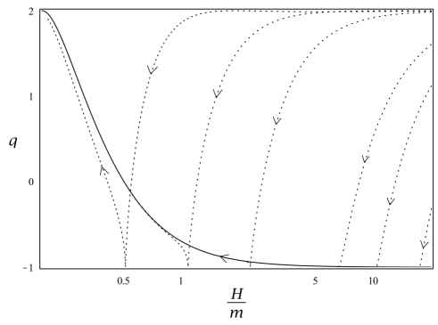
Figure 1: $H/m-q$ diagram, where $H$ is the Hubble variable and $q$ the deceleration parameter. It is seen that other solutions (dotted lines) than the attractor solution (the solid line) evolve toward the attractor solution, where the arrows denote the time direction (recall that $H/m$ is monotonically decreasing in time). The computations have been interrupted at $q=2$, since the solutions then enter the oscillatory phase.

Finally, note that ${\bf S}\rightarrow(H/m,q)$ is a surjective two-to-one map, i.e., (as can be expected) each solution only appears once in the state space of the geometric observables $(H/m,q)$ instead of twice in ${\bf S}$. It is possible to use e.g. $(T,q),\,q\in[-1,2]$ (or $(T,w_{\phi}),\,w_{\phi}\in[-1,1]$) as a bounded state space, but $q=-1$ and $q=2$ ($w_{\phi}=\pm 1$) are not invariant boundaries in such a formulation, which lead to analytic difficulties. As a consequence it is therefore preferable to use the state space ${\bf S}$, since it is bounded by invariant boundaries in an analytic manner which makes it possible to extend the state space to $\bar{\bf S}$.

To summarize the global picture of the solution space on ${\bf S}$: All orbits except for the two equivalent attractor solutions, which originate from $\mathrm{dS}_{+}$ and $\mathrm{dS}_{-}$, originate from the two equivalent sources $\mathrm{M}_{+}$ and $\mathrm{M}_{-}$, while all solutions asymptotically approach the periodic orbit on the $T=1$ invariant boundary subset, which hence is the future global attractor. This situation is depicted in Figure 2, which gives a global state space description of the solution space. Note that the heuristic description in terms of a damped harmonic oscillator does not reveal that there are two equivalent attractor solutions that originate from a de Sitter state while all other solutions originate from a massless scalar field state, nor does it reveal that the final state is one for which dimensionless physical observables such as the deceleration parameter $q$ oscillate with a constant amplitude.

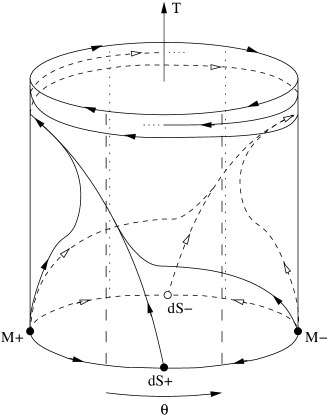
Figure 2: Examples of solutions in the global state space $\bar{\bf S}$. All solutions originate from $\mathrm{M}_{\pm}$, except for the two equivalent ‘attractor solutions’ that originate from the center saddles $\mathrm{dS}_{\pm}$. All solutions end at the limit cycle at the $T=1$ boundary at the top of the cylinder, which hence is the future global attractor. Note the strips of accelerating regions characterized by $\sin^{2}\theta<\frac{1}{3}$.

2.4 Approximations at late times

To obtain approximations for solutions at late times close to $T=1$ (the oscillatory phase), we take the average with respect to $\theta$ of the right hand side of (6) (since $-\theta\rightarrow\bar{\tau}\propto t\rightarrow\infty$ while $T$ slowly approaches one), which leads to

$$\frac{dT}{d\bar{\tau}} =\frac{3}{2}T(1-T)^{2},$$ (18a)

$$\frac{d\theta}{d\bar{\tau}} =-T.$$ (18b)

It follows that

$$\theta=-\frac{2}{3(1-T)}+C,$$ (19)

where $C=\theta_{i}+2/3(1-T_{i})$, where $(\theta_{i},T_{i})$ is some initial point for the trajectory (for heuristic work on oscillatory late time behavior for monomial scalar field potentials, see e.g. [22, 23, 24]). This approximation is valid for all solutions when $T$ approaches one, including the center manifold attractor solution, see Figure 3(a).

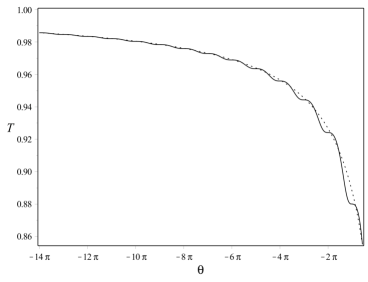
(a) The averaged solution at late times.

(b) An oscillatory approximation for the oscillatory late time regime.

Figure 3: The plot 3(a) shows the numerical attractor solution (solid line) and the averaged solution (dotted line). The plot 3(b) shows the numerical attractor solution (solid line) and the oscillatory late time approximation (dotted line).

In [9] Rendall gave rigorous results for late time behavior, which to leading order corroborates the relation given in eq. (19), but Rendall also refined this approximation. In particular he proved results that can be translated to the following asymptotic approximation [9]:

$$\theta=-t-\frac{3+2\cos(2t)}{4t},\qquad T=\left(1+\frac{2}{3(t-t_{0})}\left(1+\frac{\sin(2t)}{2t}\right)\right)^{-1},$$ (20)

where $t_{0}$ is a constant and $t$ is synchronous time (with $m$ normalized to one); note that (19) is obtained in the limit $t\rightarrow\infty$. The relations given in eq. (20) describe a parameterized curve in the global state space ${\bf S}$, which is plotted in Figure 3(b); note that the oscillatory approximation becomes increasingly good toward the future, reflecting that it describes the asymptotic evolution at late times.

Alternatively, improved late time approximations (explicitly including oscillatory behavior) can be obtained by using the averaged solution as a starting point for more accurate approximations in the manner illustrated in [25] for the case of perfect fluid dynamics in Bianchi type VII₀ at late times. These models, like the present ones, provide an example of asymptotic manifest self-similarity breaking at late times, where asymptotic (continuous) manifest self-similarity is defined by the requirement that all physical geometrical scale-invariant observables such as the deceleration parameter $q$ take asymptotic constant values (the issue of asymptotic manifest self-similarity breaking turns out to be quite subtle and we will return to it more thoroughly in a forthcoming paper). Since the future attractor in the present case is a limit cycle it follows that $q$ is asymptotically oscillating, and thus that asymptotic manifest self-similarity is broken.

Incidentally, the late time behavior in $(\phi,\dot{\phi})$-space is associated with a non-hyperbolic fixed point at the origin which acts as an attracting focus. This is rather misleading since the existence of an attracting fixed point might lead one to believe that the late time dynamics is asymptotically manifestly self-similar; the true situation, i.e. asymptotic manifest self-similarity breaking, is only revealed by resolving the non-hyperbolicity of the fixed point, which leads to the present picture with a limit cycle.

2.5 Center manifold analysis of the attractor solution

Next we will extend the center manifold analysis of [8] (a paper that was inspired by [26]), which describes the (equivalent) attractor solutions that originate from $\mathrm{dS}_{\pm}$. To do so we first briefly review some aspects of center manifold analysis that are needed for the present problem, which can be regarded as a specific application (for more details concerning center manifolds, see e.g. [16, 17]; for recent uses of center manifold analysis in cosmology, see e.g. [27, 28]).

Assume that there exists a fixed point $P$ of a dynamical system $\dot{x}=f(x)$, $x\in\mathbb{R}^{m}$ and that the linearization of the system at $P$ is described by a matrix that can be diagonalized. Accordingly, the phase space $\mathbb{R}^{m}$ of the linearized equations can be decomposed into the direct sum $E^{s}\oplus E^{u}\oplus E^{c}$ of the stable subspace $E^{s}$ (spanned by the eigenvectors of the eigenvalues with negative real parts), the unstable subspace $E^{u}$ (spanned by the eigenvectors of the eigenvalues with positive real parts) and the center subspace $E^{c}$ (spanned by the eigenvectors of the eigenvalues with vanishing real parts). These subspaces of the linearized system form the tangent spaces to associated invariant submanifolds of the full system (which therefore have the same dimension as the tangent spaces), which are denoted by $W^{s}$ for the stable manifold, $W^{u}$ for the unstable manifold, and $W^{c}$ for the center manifold.

Without loss of generality, we locate the fixed point $P$ at $(x_{1},x_{2})=(0,0)$ and choose variables such that the dynamical system can be written as

$$\dot{x}_{1} =A_{1}x_{1}+N_{1}(x_{1},x_{2}),$$ (21a)

$$\dot{x}_{2} =A_{2}x_{2}+N_{2}(x_{1},x_{2}).$$ (21b)

Here $x_{1}\in E^{c}$ is $m_{c}$-dimensional while $x_{2}\in E^{s}\oplus E^{u}$ is ($m_{u}+m_{s}$)-dimensional; $A_{1}$ is a constant $m_{c}\times m_{c}$ matrix with purely imaginary (or zero) eigenvalues; $A_{2}$ is a constant $(m_{s}+m_{u})\times(m_{s}+m_{u})$ matrix for which all eigenvalues have nonzero real parts; finally, $N_{1}$ and $N_{2}$ denote the nonlinear terms.

Since the center manifold $W^{c}$ is an invariant manifold in the phase space $\mathbb{R}^{m}$ that contains $P$ and that is tangent to $E^{c}$, one can describe $W^{c}$, in a neighborhood of $P$, as the graph of a function $h:E^{c}\rightarrow E^{s}\oplus E^{u}$, i.e., $x_{2}=h(x_{1})$, where for sufficiently small $x_{1}$ the point $(x_{1},h(x_{1}))$ belongs to $W^{c}$. Inserting the relation $x_{2}=h(x_{1})$ into (21) yields the following differential equation for $h$:

$$\partial_{x_{1}}h(x_{1})\>[A_{1}x_{1}+N_{1}(x_{1},h(x_{1}))]=A_{2}h(x_{1})+N_{2}(x_{1},h(x_{1})),$$ (22)

which also satisfies $h(0)=0$ (fixed point condition) and $(\partial_{x_{1}}h)(0)=0$ (tangency condition). Usually, however, it is not possible to solve (22). Instead this equation can be solved approximately by representing $h(x_{1})$ as a formal (usually truncated) power series, and solve for the constant coefficients to any desired order.

The Hartman-Grobman theorem can be generalized to the Shoshitaishvili theorem (sometimes referred to as the reduction theorem) for the present situation of a non-hyperbolic fixed point:

Theorem 2.1.

(Shoshitaishvili theorem). Consider the dynamical system (21) in a neighborhood of the fixed point $P=(0,0)$. The flow of the full nonlinear system and the flow of the reduced system

$$\dot{x}_{1} =A_{1}x_{1}+N_{1}(x_{1},h(x_{1}))$$ (23a)

$$\dot{x}_{2} =A_{2}x_{2}\>.$$ (23b)

are locally equivalent, i.e., there exists a local homeomorphism $\Psi$ on phase space, such that $\phi_{t}^{\mathrm{full}}=\Psi^{-1}\circ\phi_{t}^{\mathrm{reduced}}\circ\Psi$. Here, $h$ is given by (22).

Note that $x_{2}=0$ forms an invariant subset of (23) that describes the center manifold.

Let us now apply the above to the global dynamical system (6). Due to the discrete symmetry it suffices to investigate one of the non-hyperbolic $\mathrm{dS}_{\pm}$ fixed points, and without loss of generality it is convenient to choose the $\mathrm{dS}_{+}$ fixed point at $(T,\theta)=(0,0)$. The starting point for a center manifold analysis is a linearization of the system at the fixed point, which in the present case leads to the eigenvalues $-3$ and zero and the following stable, $E^{s}$, and center, $E^{c}$, tangential subspaces, respectively:

$$E^{s} =\{(T,\theta)|T=0\},$$ (24a)

$$E^{c} =\{(T,\theta)|T+3\theta=0\}.$$ (24b)

Since the tangential center subspace is given by $T+3\theta=0$, we introduce $v=T+3\theta$ as a new variable in order to study the center manifold $W^{c}$ (with the tangent space $E^{c}$ at $(T,v)=(0,0)$). As follows from (6), this leads to the transformed system

$$\frac{dT}{d\bar{\tau}} =3T(1-T)^{2}\sin^{2}\left({\textstyle{1\over 3}}(v-T)\right),$$ (25a)

$$\frac{dv}{d\bar{\tau}} =3\left(T(1-T)^{2}\sin^{2}\left({\textstyle{1\over 3}}(v-T)\right)-T-\frac{3}{2}(1-T)\sin\left({\textstyle{2\over 3}}(v-T)\right)\right).$$ (25b)

Note that the linearization of eq. (25b) yields $\frac{dv}{d\bar{\tau}}=-3v$, while eq. (25a) only has higher order terms, which corresponds to the eigenvalues $-3$ and zero. The center manifold $W^{c}$ can be obtained as the graph $v=h(T)$ near $(T,v)=(0,0)$ (i.e., use $T$ as an independent variable), where $h(0)=0$ (fixed point condition) and $\frac{dh}{dT}(0)=0$ (tangency condition). Inserting this relationship into eq. (25) and using $T$ as the independent variable leads to

$$T(1-T)^{2}\sin^{2}\left({\textstyle{1\over 3}}(h-T)\right)\left(\frac{dh}{dT}-1\right)+T+\frac{3}{2}(1-T)\sin\left({\textstyle{2\over 3}}(h-T)\right)=0.$$ (26)

Not surprisingly it is hard to solve this differential equation since this would amount to actually finding the center manifold, i.e., in this case the attractor solution. However, we can solve the equation approximately by representing $h(T)$ as the formal power series

$$h(T)=\sum_{i=2}^{n}a_{i}T^{i}+{\cal O}(T^{n+1})\qquad\text{as}\qquad T\rightarrow 0,$$ (27)

where the series for $h(T)$ is truncated at some chosen order $n$. Inserting this into eq. (26) and algebraically solving for the coefficients leads to that $\theta=\frac{1}{3}(-T+h(T))$ is given by

$$\begin{split}\theta&=-\frac{1}{3}\left\{T+T^{2}+\underbrace{\frac{26}{3^{3}}}_{0.963}T^{3}+\underbrace{\frac{8}{3^{2}}}_{0.889}T^{4}+\underbrace{\frac{107}{3^{3}\cdot 5}}_{0.793}T^{5}+\underbrace{\frac{19}{3^{3}}}_{0.704}T^{6}\right.\\ &\\ &\qquad\left.+\underbrace{\frac{3352}{3^{6}\cdot 7}}_{0.657}T^{7}+\underbrace{\frac{490}{3^{6}}}_{0.672}T^{8}+\underbrace{\frac{43381}{3^{10}}}_{0.735}T^{9}+\underbrace{\frac{25961}{3^{8}\cdot 5}}_{0.791}T^{10}\right\}+{\cal O}(T^{11}),\end{split}$$ (28)

where we have chosen to expand $h(T)$ to 10th order. Figure 4 depicts the numerical description of the attractor solution and plots of curves associated with expansions to various orders obtained from (28) (to avoid clutter we do not give all expansions up to 10th order, but each order gives a more accurate approximation than the previous one). As is seen from this figure, and Table 1, higher order expansions yield increasingly better approximations for the attractor solution, even far from $(T,\theta)=(0,0)$, indicating quite good convergence for rather large $T$, i.e., small $H/m$, even beyond the end of inflation, i.e., beyond $q=0$ (although it is only at second order or higher that $q=0$ is actually passed).

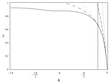
(a) Center manifold expansions.

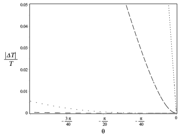
(b) Relative errors for center manifold expansions.

Figure 4: The plot 4(a) shows the state space $(T,\theta)$, with $\theta$ in the range $[-2\pi,0]$, with the numerical solution (solid line) and the center manifold expansion ($\mathrm{CMexp}$) to 1st (dotted), 2nd (dashed), 6th (space-dotted), and 10th (space-dashed) order approximation. The end of the accelerating regime, $q=0$, is depicted by the vertical line. The plot 4(b) shows the relative errors $|\Delta T|/T=|T_{\mathrm{CMexp}}-T_{\mathrm{num}}|/T_{\mathrm{num}}$ for the center manifold expansions for small $\theta$ (and hence for small $T$).

	Num.	1st	2nd	6th	10th
$T$	0.6646	—	0.9479	0.6842	0.6682
$\frac{|\Delta T|}{T}$	—	—	42.627%	2.949%	0.542%
$\frac{H}{m}$	0.5047	—	0.0550	0.4616	0.4967
$\frac{|\Delta H|}{H}$	—	—	89.112%	8.538%	1.595%

Table 1: Numerical values and relative errors for center manifold expansions at $q=0$. The relative errors are given by $|\Delta T|/T=|T_{\mathrm{CMexp}}-T_{\mathrm{num}}|/T_{\mathrm{num}}$ and $|\Delta H|/H=|H_{\mathrm{CMexp}}-H_{\mathrm{num}}|/H_{\mathrm{num}}$ .

2.6 Padé approximants for the attractor solution

To obtain a better range and rate of convergence we will replace the above center manifold expansions in eq. (28) with so-called Padé approximants (for more details, see e.g. [27, 29, 30], and for some recent examples in cosmology, see [31, 32]). A Padé approximant is a particular approximation of a function at a regular point by a rational function. The Padé approximant of order $(m,n)$ of a function $f(x)$, denoted by $[m/n]_{f}(x)$, is associated with a truncated Taylor series (where we without loss of generality assume that the regular point we are interested in is located at $x=0$, i.e., we perform a truncated Maclaurin series expansion):

$$f\approx c_{0}+c_{1}x+c_{2}x^{2}+\cdots+c_{m+n}x^{m+n},$$ (29)

and given by the polynomials $P_{m}(x)$ and $Q_{n}(x)$ according to

$$[m/n]_{f}(x)=\frac{P_{m}(x)}{Q_{n}(x)}=\frac{p_{0}+p_{1}x+p_{2}x^{2}+\cdots+p_{m}x^{m}}{q_{0}+q_{1}x+q_{2}x^{2}+\cdots+q_{n}x^{n}},$$ (30)

such that

$$Q_{n}(x)(c_{0}+c_{1}x+c_{2}x^{2}+\cdots+c_{m+n}x^{m+n})=P_{m}(x),$$ (31)

where coefficients with the same powers of $x$ are equated up through $m+n$. Thus

$$\sum_{j=0}^{n}q_{j}c_{m-j+k}=0, \qquad k =1,\dots,n,$$ (32a)

$$\sum_{j=0}^{k}q_{j}c_{k-j}-p_{k}=0, \qquad k =0\dots,m,$$ (32b)

yields a system of $m+n+1$ linear equations in $m+n+2$ unknowns $p_{0},\dots,p_{m}$ and $q_{0},\dots,q_{n}$ (writing the above linear system, which defines the Padé approximant, as a matrix equation reveals that the defining matrix takes a very special form, namely that of a Töplitz matrix). This therefore leads to several possible solutions, but the possible expressions for $[m/n]_{f}(x)$ only differ by a common factor in $P_{m}(x)$ and $Q_{m}(x)$ and one can therefore without loss of generality scale these polynomials to set $q_{0}=1$ (the so-called Baker condition; for a discussion concerning this normalization, see [30]), which yields the standard form for the Padé approximant $[m/n]_{f}(x)$. This, however, assumes that $Q_{n}(0)\neq 0$, while problems arise if $Q_{n}(0)=0$. In this paper we will avoid such difficulties and compute Padé approximants with $q_{0}=1$. It should also be pointed out that there are more efficient ways of computing Padé approximants than the just outlined one, although for our purposes the above suffices.

Why are Padé approximants interesting? By definition it follows that

$$Q_{n}(x)f(x)-P_{m}(x)={\cal O}(x^{m+n+1}),$$ (33)

Padé approximants therefore agree with the truncated power series of the function it approximates up to the power $m+n$ (a Padé approximant can be viewed as a generalization of a Taylor polynomial which can be associated with the above equation by formally setting $Q_{n}(x)=1$). Nevertheless, the difference between the Taylor series and the associated Padé approximants is crucial, since the latter often works better than the power series, i.e., Padé approximants often have a better rate and range of convergence. This is illustrated by the present paper; below we will use Padé approximants for the center manifold expansion associated with $\mathrm{dS}_{+}$, and, as will be seen, the Padé approximants give significantly better results than their associated Taylor series approximations. In this context it should be pointed out that although there exists a number of convergence results in the literature, these are not suitable for determining the precise quantitative convergence properties of a given function, or the differential equation that defines it, which in the present case is eq. (26) for $h(T)$ (at least the authors have not found any theorem that is directly applicable in the present context). It is for this reason we will give our results below in the form of plotted errors. Finally, note that the generalization of a Padé approximant to an approximant in several variables is called a Canterbury approximant.

Instead of producing the Padé approximants associated with the expansion (28), we will give the Padé approximants that arise from the analogous expression of the dynamical system (15) in Section 2.2 which is adapted to the particular structures exhibited at early times. The reason for this is that this will yield the odd Padé approximants obtained from the $T$ expansion (28), but with less computation and in a succinct form. Furthermore, the even Padé expressions, $[2/2]_{\theta}$, $[4/4]_{\theta}$, obtained from eq. (28), do not converge for large $T$ (in contrast to the center manifold series expansions, which do converge for large $T$), and we therefore refrain from giving them. To obtain the relevant Padé approximants we first have to calculate the center manifold expansion of $\mathrm{dS}_{+}$ of the dynamical system (15) for the dependent variables $\theta$ and $\tilde{T}$, where we recall that ${\tilde{T}}$ is defined by

$$\tilde{T}=\frac{T}{1-T}=\frac{m}{H}.$$ (34)

In this case we obtain

$$E^{s} =\{(\tilde{T},\theta)|\tilde{T}=0\},$$ (35a)

$$E^{c} =\{(\tilde{T},\theta)|\tilde{T}+3\theta=0\}.$$ (35b)

The graph representation of the center manifold $W^{c}$ is given by $\tilde{T}+3\theta=\tilde{h}(\tilde{T})$ near $(\tilde{T},\theta)=(0,0)$, where, as follows from eq. (15), $\tilde{h}(\tilde{T})$ obeys the first order ordinary differential equation

$$\tilde{T}\sin^{2}\left({\textstyle{1\over 3}}(\tilde{h}-\tilde{T})\right)\left(\frac{d\tilde{h}}{d\tilde{T}}-1\right)+\tilde{T}+\frac{3}{2}\sin\left({\textstyle{2\over 3}}(\tilde{h}-\tilde{T})\right)=0.$$ (36)

Representing $\tilde{h}(\tilde{T})$ by a formal power series and inserting this into (36) yields that $\theta=\frac{1}{3}(-\tilde{T}+\tilde{h}(\tilde{T}))$ can be written as

$$\theta=-\frac{1}{3}\tilde{T}\left\{1-\underbrace{\frac{1}{3^{3}}}_{0.037}\tilde{T}^{2}+\underbrace{\frac{2}{3^{3}\cdot 5}}_{0.015}\tilde{T}^{4}-\underbrace{\frac{50}{3^{6}\cdot 7}}_{0.010}\tilde{T}^{6}+\underbrace{\frac{532}{3^{10}}}_{0.009}\tilde{T}^{8}\right\}+{\cal O}(\tilde{T}^{11}),$$ (37)

when $\tilde{h}(\tilde{T})$ is expanded to 10th order. Figure 5 shows that the center manifold expansion in $\tilde{T}$ converges for small $T$ ($\tilde{T}<1\,\rightarrow\,T<1/2$), but not for large $T$ (thus this formulation gives a center manifold expansion with smaller range of convergence than the previous results in $T$).

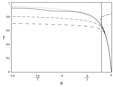
(a) Center manifold expansions in $\tilde{T}$

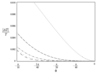
(b) Relative errors for the center manifold expansions in $\tilde{T}$

Figure 5: The plot 5(a) shows the state space $T,\theta$, with $\theta$ in the range $[-2\pi,0]$, with the numerical solution (solid line) and the center manifold expansion in $\tilde{T}$ to 1st (dotted), 2nd (dashed), 3rd (dash-dotted), 7th (space-dotted), and 10th (space-dashed) order approximation. The end of inflation, $q=0$, is depicted by the vertical line. The plot 5(b) shows the relative errors $|\Delta T|/T$ for the center manifold expansions for small $\theta$.

Expressing (37) in $T$ yields a rational function, which when expanded to 10th order precisely gives (28), which converges for larger values than $T=1/2$. Next we turn to Padé approximants. Writing (37) as $\theta=-\frac{1}{3}\tilde{T}f(\tilde{T}^{2})$ and writing $f(\tilde{T}^{2})$ in terms of its Padé approximants for the various orders yield

$$[1/1]_{\theta} =-\frac{\tilde{T}}{3}f(0)=-\frac{\tilde{T}}{3},$$ (38a)

$$[3/3]_{\theta} =-\frac{\tilde{T}}{3}[1/1]_{f}=-\frac{\tilde{T}}{3}\left(\frac{1+\frac{7^{2}}{3^{3}\cdot 5}\tilde{T}^{2}}{1+\frac{2}{5}\tilde{T}^{2}}\right),$$ (38b)

$$[5/5]_{\theta} =-\frac{\tilde{T}}{3}[2/2]_{f}=-\frac{\tilde{T}}{3}\left(\frac{1+\frac{61\cdot 419}{3^{4}\cdot 13\cdot 19}\tilde{T}^{2}+\frac{2^{4}\cdot 167\cdot 1609}{3^{4}\cdot 5\cdot 7\cdot 13\cdot 19}\tilde{T}^{4}}{1+\frac{2^{2}\cdot 5^{2}\cdot 263}{3^{4}\cdot 13\cdot 19}\tilde{T}^{2}+\frac{2\cdot 5\cdot 3659}{3^{4}\cdot 7\cdot 13\cdot 19}\tilde{T}^{4}}\right),$$ (38c)

where the notation on the right hand side corresponds to the Padé expression for $\theta(T)$ obtained from the series expansion (37). Thus using the center manifold expansion associated with $\mathrm{dS}_{+}$ for the dynamical system (15) is a computationally convenient way of obtaining the ‘natural’ convergent series of Padé approximants in a compressed form for the center manifold of $\mathrm{dS}_{+}$ of the dynamical system (6). In eq. (38) each expression gives a curve in the state space ${\bf S}$ that approximates the attractor solution, when $\tilde{T}$ is replaced by $T$. The numerical solution and the above Padé approximants are plotted together with relative errors, $|\Delta T|/T=|T_{\mathrm{Pad}}-T_{\mathrm{num}}|/T_{\mathrm{num}}$, in Figure 6. In addition we give the relative errors $|\Delta T|/T$ and $|\Delta H|/H$ of the center manifold Padé approximants at the end of the accelerating regime, i.e., at $q=0$, in Table 2. As can be seen, increasingly higher Padé approximants give better results, indicating desirable convergence and range properties. Moreover, note that the Padé approximants yield much better results than the associated series expansions described in Section 2.5.

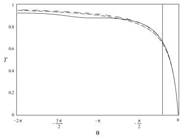
(a) Padé approximants in ${\bf S}$.

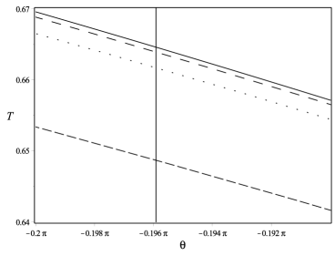
(b) Padé approximants near $q=0$.

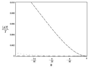
(c) Relative errors of Padé approximants for small $\theta$

Figure 6: The plot 6(a) shows the numerical solution (solid line) and the $[1/1]_{\theta}$ (dashed), $[3/3]_{\theta}$ (space-dotted), and $[5/5]_{\theta}$ (space-dashed) Padé approximants in the state space ${\bf S}$. The plot 6(b) depicts the situation close to $q=0$ (the vertical line) in more detail. The plot 6(c) shows the relative errors for the Padé approximants.

	Num.	$[1/1]_{\theta}$	$[3/3]_{\theta}$	$[5/5]_{\theta}$
$T$	0.6646	0.6487	0.6617	0.6639
$\frac{|\Delta T|}{T}$	—	2.392%	0.436%	0.102%
$\frac{H}{m}$	0.5047	0.5416	0.5113	0.5062
$\frac{|\Delta H|}{H}$	—	7.308%	1.299%	0.298%

Table 2: Numerical values and relative errors for the Padé approximants at $q=0$.

2.7 Global approximations

Thanks to the large range of the center manifold based Padé approximants these can be joined with the approximations for the evolution at late times to yield temporally global approximations for the attractor solution. In Figure 7(a) the $[3/3]_{\theta}$ approximant, given in eq. (38), is matched with the average approximation for late times, given in eq. (19), to yield a global piecewise approximation for the attractor solution. Figure 7(b) depicts a temporally global description of the attractor solution obtained by joining the $[3/3]_{\theta}$ Padé approximant with the late time approximation given in eq. (20).

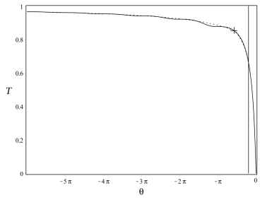
(a) Global piecewise Padé-averaged approximation.

(b) Matched global Padé-oscillatory approximation.

Figure 7: The plot 7(a) shows the numerical solution (solid line) and the $[3/3]_{\theta}$ Padé approximant matched (at the cross) with the averaged solution where the $[3/3]_{\theta}$ Padé approximant crosses the numerical solution at $T\approx 0.8552$. The plot 7(b) shows the numerical solution (solid line) and the $[3/3]_{\theta}$ Padé approximant matched with the approximate oscillatory solution for late times (at the cross, where $T\approx 0.8552,\,t_{0}\approx-2.1212$).

Note that an approximate solution for the entire attractor solution, which subsequently can be used to obtain an approximate solution in e.g. $(\phi,\dot{\phi})$-space, may make it possible to at least approximately obtaining or estimating a global measure [18] in $(\phi,\dot{\phi})$-space (or $(T,\theta)$-space for $T\in(0,1)$) that might shed further light on the meaning of an ‘attractor solution.’

Finally, it is worth pointing out that one can also obtain approximations for the remaining solutions that originate from the hyperbolic fixed points $\mathrm{M}_{\pm}$ by series expansions of these fixed points based on Picard’s method, as described in the Bianchi type II perfect fluid case in [33], see also references therein and [34]. These expansions can be used to obtain approximants in order to improve the rate and range of convergence, and it is thereby possible to approximately describe the entire solution space. A similar statement holds for a wide range of related problems in General Relativity and modified gravity theories; again, we stress that the current minimally coupled scalar field with a quadratic potential just serves as an illustrative example.

3 Slow-roll and center manifold approximant comparisons

The purpose with this section is twofold: (i) to use the present example with a quadratic potential to clarify the slow-roll approximation and its expansion extensions, showing that the so-called slow-roll approximation actually corresponds to several approximations for the attractor solution (this is a point that is related to the ones raised in the recent paper [35] as regards so-called horizon-flow approximations), (ii) to quantitatively assess the accuracy of slow-roll approximations for the present quadratic scalar field potential. In forthcoming papers we will generalize and contextualize these results to increasingly general situations; in particular we will in a subsequent paper deal with monomial potentials and perfect fluids as the source.

To discuss slow-roll approximants we first reproduce and extend the results by Liddle et al. [10] who introduced a hierarchy of Hubble slow-roll parameters, which were subsequently related to a hierarchy of potential slow-roll parameters in order to produce analytic slow-roll expansions and approximants. In terms of our state space variables the first two Hubble slow-roll parameters are given by

$$\epsilon_{H}=1+q=3\sin^{2}\theta,\qquad\eta_{H}=3+\left(\frac{T}{1-T}\right)\cot\theta.$$ (39)

To facilitate comparisons with [10] we here keep the coupling constant $\kappa=8\pi m^{-2}_{\mathrm{Pl}}$. Following the methods described in [10] results in that to 4th order for the present quadratic potential the slow-roll expansion for $(H/m)^{2}$ in $\phi^{2}$ is given by

$$\left(\frac{H}{m}\right)^{2}=\frac{\kappa\phi^{2}}{6}\left[1+\frac{2}{3\kappa\phi^{2}}-\frac{2^{2}}{3^{2}\kappa^{2}\phi^{4}}+\frac{2^{5}}{3^{3}\kappa^{3}\phi^{6}}-\frac{2^{4}\cdot 5^{2}}{3^{4}\kappa^{4}\phi^{8}}+{\cal O}\left(\frac{1}{\kappa^{5}\phi^{10}}\right)\right].$$ (40)

while the first so-called Canterbury approximants, based on slow-roll potential parameters as described in [10], are given by

$$[1/1] =\frac{\kappa\phi^{2}}{6}\left[\frac{1+\frac{2^{2}}{3\kappa\phi^{2}}}{1+\frac{2}{3\kappa\phi^{2}}}\right],$$ (41a)

$$[2/2] =\frac{\kappa\phi^{2}}{6}\left[\frac{1+\frac{13}{2\kappa\phi^{2}}+\frac{2\cdot 5^{2}}{3^{2}\kappa^{2}\phi^{4}}}{1+\frac{5\cdot 7}{2\cdot 3\kappa\phi^{2}}+\frac{19}{3^{2}\kappa^{2}\phi^{4}}-\frac{7\cdot 2^{2}}{3^{3}\kappa^{4}\phi^{8}}-\frac{2\cdot 7\cdot 13}{3^{3}\kappa^{5}\phi^{10}}-\frac{2^{3}\cdot 5^{2}\cdot 7}{3^{5}\kappa^{6}\phi^{12}}}\right].$$ (41b)

The slow-roll expansions and Canterbury approximants are compared with the numerical attractor solution in Figure 8. For large $\phi$, and thereby large $H$, there is convergence for the series expansions, but this is no longer the case for small $\phi$. Furthermore, note that the best approximant for small $\phi$ is the $[1/1]$ approximant. The same holds for the plot of $\epsilon_{H}=-\frac{d\ln H}{d\ln a}=3\dot{\phi}^{2}/(\dot{\phi}^{2}+m^{2}\phi^{2})$ versus $\phi/m_{\mathrm{Pl}}$ given in Figure 9.

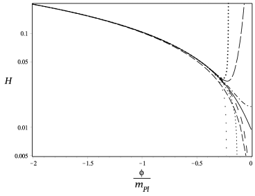
(a) Hubble slow-roll approximants

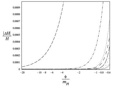
(b) Hubble slow-roll errors

Figure 8: The plot 8(a) describes the numerical solution (solid line) and the Hubble slow-roll approximants (in this plot $m$ has been chosen so that the lower order approximants yield the results in [10]). The plot 8(b) gives the relative errors of the Hubble slow-roll approximants for large values of $\phi$. Both plots depict the 0th (dashed), 1st (dot-dashed), 2nd (dotted), 3rd (long-dashed), and 4th (space-dotted) order approximations, and the $[1/1]$ (space-dashed) and $[2/2]$ (fat-dotted) Canterbury approximants.

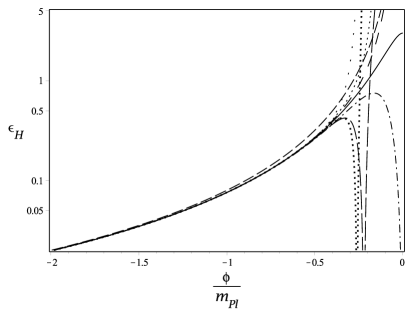
Figure 9: $\epsilon_{H}(\phi/m_{\mathrm{Pl}})$: The notation for the various curves is the same as in the previous figures.

In the present context, it follows from eq. (39) that the slow-roll limit $\epsilon_{H}=\eta_{H}=0$ corresponds to the fixed points $\mathrm{dS}_{\pm}$ and that only imposing ‘the attractor condition’ $\eta_{H}=0$ close to (without loss of generality) $(T,\theta)=(0,0)$ yields $T+3\theta=0$, i.e., the attractor condition leads to the tangent space $E^{c}$ of the center manifold solution in the slow-roll limit. It therefore follows that the slow-roll expansions in [10] corresponds to an analytic attempt to describe the center manifold, i.e., the attractor solution, to increasing accuracy, which in turn describes the intermediate time behavior of an open set of solutions that passes close to the de Sitter fixed point (where measures attempt to describe how ‘large’ this open set is).

Slow-roll approximations actually consist of two classes of approximations. The first class of approximations arises from obtaining approximate expressions for $H^{2}(\phi)$. These are the so-called Hubble slow-roll expansions given in eq. (40) and the associated Canterbury approximants given in eq. (41), which give rise to a family of curves in ${\bf S}$ which yield approximations for the attractor solution. These approximation curves are obtained by performing the transformation (10) (after having set $8\pi m_{\mathrm{Pl}}^{-2}=1$). The curves and relative errors for various series expansions and approximants are given in Figure 10 together with the numerically calculated attractor solution; in addition we describe numerical values and relative errors at $q=0$ in Table 3. Note that to zeroth order the Hubble expansion gives $\cos^{2}\theta=1$, which corresponds to the straight lines in $\bar{\bf S}$ describing $q=-1$.

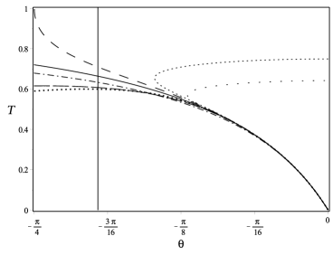
(a) Hubble slow-roll approximations.

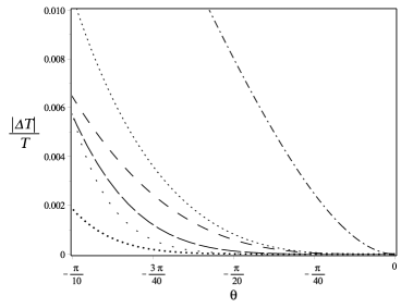
(b) Relative errors for Hubble slow-roll approximations.

Figure 10: The plot 10(a) describes the numerical solution (solid line) and the different Hubble slow-roll approximations: the 1st (dot-dashed), 2nd (dotted), 3rd (long-dashed), and 4th (space-dotted) order approximations, and the [1/1] (space-dashed) and [2/2] (fat-dotted) Canterbury approximants. The plot 10(b) gives the relative errors for the Hubble slow-roll approximations.

	Num.	0th	1st	2nd	[1/1]	3rd	4th	[2/2]
$T$	0.6646	—	0.6340	—	0.7101	0.6083	—	0.6002
$\frac{|\Delta T|}{T}$	—	—	4.604%	—	6.846%	8.471%	—	9.690%
$\frac{H}{m}$	0.5047	—	0.5774	—	0.4082	0.6440	—	0.6660
$\frac{|\Delta H|}{H}$	—	—	14.400%	—	19.111%	27.598%	—	31.952%

Table 3: Numerical values and relative errors for Hubble slow-roll expansions and Canterbury approximants at $q=0$.

As can be seen from Figure 10, the Hubble series expansion converge for small $T$ (i.e., large $H$), which is the slow-roll regime, but not for large $T$ (i.e. small $H$), as can be expected. The [2/2] Canterbury approximant is the best approximation for small $T$, while the 1st order Hubble expansion approximation is the most accurate among the slow-roll approximants for large $T$ at $q=0$, see Figure 10 and Table 3. This is to be contrasted with the center manifold expansions and the odd Padé approximants which converge even beyond the inflationary stage, far from where the slow-roll conditions break down. It is this larger range of convergence that makes it possible to obtain quite good piecewise global approximations for the attractor solution by matching center manifold based approximants with approximations for the evolution at late times, as shown in the previous section.

When comparing the 1st order Hubble expansion approximant with the center manifold approximants in Figure 11(a) it is seen that the 6th order center manifold expansion and the $[1/1]_{\theta}$ Padé approximant yields a more accurate approximation for the attractor solution than the 1st order Hubble expansion approximation everywhere, although especially for large $|\theta|$ and $T$. Furthermore, in Figure 11(b) it is shown that the $[5/5]_{\theta}$ Padé approximant gives a better approximation for the attractor solution than the $[2/2]$ Canterbury approximant everywhere, especially for large $|\theta|$ and $T$, while the $[3/3]_{\theta}$ Padé approximant is better than the $[2/2]$ Canterbury approximant everywhere except for quite small $|\theta|$ and $T$.

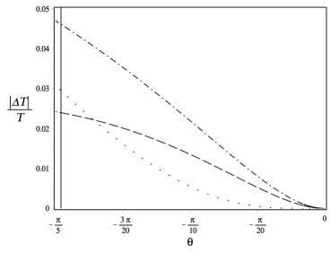
(a) Relative errors: 1st order Hubble expansion approximation and center manifold approximants

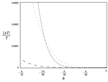
(b) Relative errors: Hubble expansion Canterbury approximant and center manifold approximants

Figure 11: The plot 11(a) describes the relative errors for the the 1st order Hubble expansion approximation (dash-dotted); the 6th order center manifold expansion (space-dotted); the $[1/1]_{\theta}$ Padé approximant (dashed). The plot 11(b) describes the relative errors of the $[2/2]$ Canterbury approximant (fat dotted); the $[3/3]_{\theta}$ Padé approximant (space-dotted); the $[5/5]_{\theta}$ Padé approximant (space-dashed).

The second class of slow-roll approximations for the attractor solution arises from inserting the first class of Hubble expansion and Canterbury approximants into

$$\dot{\phi}=-2\frac{\partial H}{\partial\phi}$$ (42)

(obtained by using $\phi$ locally as the independent variable and using the present units). The usual slow-roll aproximation is obtained by inserting the zeroth order Hubble expansion approximation into the above equation [36], which for the present models yields the same expression as the 1st order Hubble expansion approximation given previously (cf. Tables 3 and 4) and which we have compared with center manifold approximants in Figure 11(a). (For the present models, the 1st $\dot{\phi}$ slow-roll approximation also gives the $[1/1]$ Hubble slow-roll approximation.)

It is of interest to note that the slow-roll approximation and the $[1/1]_{\theta}$ Padé approximant yield the following expressions for the deceleration parameter $q$ as a function of $H/m$:

$$q =-1+\frac{1}{3}\left(\frac{m}{H}\right)^{2} (\text{slow-roll}),$$ (43a)

$$q =-1+3\sin^{2}\left[\frac{1}{3}\left(\frac{m}{H}\right)\right] ([1/1]_{\theta}\,\,\text{Pad\'{e}}).$$ (43b)

These expressions have been plotted in Figure 12 together with the attractor solution.

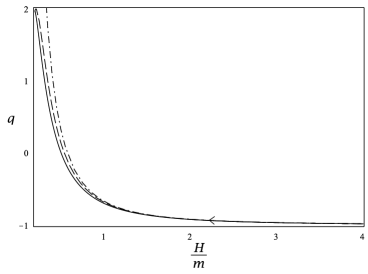
Figure 12: The plot describes $q(H/m)$ for the slow-roll approximation (dash-dotted); the $[1/1]_{\theta}$ Padé approximant (dashed); and the numerical attractor solution (solid line).

As shown in Figure 13, the approximations based on (42) are more accurate than the Hubble expansions for small $T$, except for the previous $[2/2]$ Canterbury approximant, but, as in the case of slow-roll Hubble expansions and Canterbury approximants, the center manifold expansions and Padé approximants yield better results for the attractor solution for large $T$, as can be seen by comparing Tables 1 and 2 with Table 4 for $q=0$.

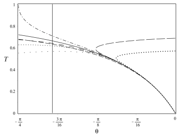
(a) $\dot{\phi}$ slow-roll approximations.

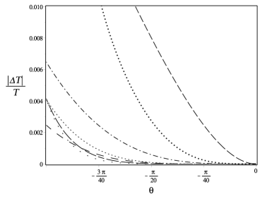
(b) Relative errors for the $\dot{\phi}$ slow-roll approximations.

Figure 13: Numerical solution (solid line) and $\dot{\phi}$ slow-roll approximations to 0th (dashed), 1st (dot-dashed), 2nd (dotted), 3rd (long-dashed), and 4th (space-dotted) order approximation, and the [1/1] (space-dashed) and [2/2] (fat-dotted) Canterbury approximants.

	Num.	0th	1st	2nd	[1/1]	3rd	4th	[2/2]
$T$	0.6646	0.6340	0.7101	0.6186	0.6420	—	0.5676	—
$\frac{|\Delta T|}{T}$	—	4.604%	6.846%	6.923%	3.400%	—	14.602%	—
$\frac{H}{m}$	0.5047	0.5774	0.4083	0.6166	0.5576	—	0.7619	—
$\frac{|\Delta H|}{H}$	—	14.400%	19.111%	22.168%	10.487%	—	50.969%	—

Table 4: Numerical values and relative errors for the various $\dot{\phi}$ slow-roll expansions and Canterbury approximants at $q=0$.

Among the two classes of slow-roll approximations, the $[1/1]$ slow-roll Canterbury $\dot{\phi}$ approximant is the best one for large $T$. However, as can be seen from Figure 14, the $[3/3]_{\theta}$ Padé approximant is a more accurate approximation than the $[1/1]$ Canterbury $\dot{\phi}$ slow-roll approximation everywhere, while the $[1/1]_{\theta}$ Padé approximant gives a better result for large $|\theta|$ and $T$.

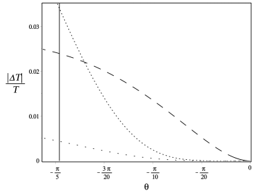
Figure 14: The plot describes the relative errors for the $[1/1]$ Canterbury $\dot{\phi}$ slow-roll approximation (dotted); the $[1/1]_{\theta}$ Padé approximant (space-dashed); the $[3/3]_{\theta}$ Padé approximant (space-dotted).

4 Concluding remarks

In this paper we have used the minimally coupled scalar field with a quadratic potential in flat FLRW cosmology to illustrate how a global dynamical system can yield a global understanding of the solution space as well as the solution’s asymptotic features. We have also used center manifold expansions and Padé approximants to obtain approximations for the attractor solution at early times. In addition we have showed that late time asymptotics for all solutions is associated with a limit cycle that demonstrates that the present models exhibit future asymptotic manifest self-similarity breaking, which physically corresponds to that physical dimensionless observables such as the deceleration parameter have no future asymptotic limits, but instead oscillate. This is an issue that becomes even more pertinent when one includes additional sources such as perfect fluids and we will return to this in a forthcoming paper dealing with scalar fields with monomial potentials and perfect fluids. In this case there is a ‘competition’ between the different matter sources, reminiscent of the dynamics of Lotka-Volterra systems, as described in [37].

In addition we have shown that the slow-roll approximation and expansions are actually a collage of two types of approximations that describe the early behavior of the attractor solution. These approximations were subsequently compared with the center manifold approximations. It was found that center manifold expansions and associated approximants have a larger range of convergence than the slow-roll approximation and associated approximants. Furthermore, it was shown that the $[1/1]_{\theta}$ Padé approximant gives a better approximation than the slow-roll approximation to the attractor solution everywhere. The large range of convergence for center manifold approximants made it possible to join them with approximations describing the dynamics at late times to produce global approximations for the attractor solution.

Different convergence properties of various approximation schemes might have far reaching consequences, so let us therefore take a closer look at the slow-roll approximation. Expressed in $\theta$ and $T$ the slow-roll approximation takes the following form for the quadratic scalar field potential:

$$\theta_{\mathrm{SR}}=-\arcsin{\left(\frac{T}{3(1-T)}\right)}.$$ (44)

Performing a Taylor expansion around $T=0$ yields

$$\begin{split}\theta_{\mathrm{SR}}&=-\frac{1}{3}\left\{T+T^{2}+\underbrace{\frac{55}{2\cdot 3^{3}}}_{1.019}T^{3}+\underbrace{\frac{19}{2\cdot 3^{2}}}_{1.056}T^{4}-\underbrace{\frac{1201}{2^{3}\cdot 3^{3}\cdot 5}}_{1.112}T^{5}+\underbrace{\frac{257}{2^{3}\cdot 3^{3}}}_{1.190}T^{6}\right.\\ &\\ &\qquad\left.+\underbrace{\frac{105467}{2^{4}\cdot 3^{6}\cdot 7}}_{1.292}T^{7}+\underbrace{\frac{16583}{2^{4}\cdot 3^{6}}}_{1.422}T^{8}+\underbrace{\frac{11980259}{2^{7}\cdot 3^{10}}}_{1.585}T^{9}+\underbrace{\frac{7510063}{2^{7}\cdot 3^{8}\cdot 5}}_{1.789}T^{10}\right\}+{\cal O}(T^{11}).\end{split}$$ (45)

A comparison with the center manifold expansion given in eq. (28) shows that it is only the first two terms that coincide. For every other order the errors for the slow-roll expansion in (45) are larger than those in (28), and a similar statement holds for the associated Padé approximants. It is only the exact translations of the slow-roll Hubble expansions and Canterbury approximants that give competitive results for small $T$ when compared with the lower order center manifold expansions, which in turn corresponds to nonlinear variable transformations between $(\phi,H)$ and $(\theta,T)$.

Thus the present paper provides specific examples of how nonlinear transformations and different approximation schemes significantly affects convergence rates and ranges for flat FLRW cosmology with a minimally coupled scalar field with a quadratic potential, which should not come as a surprise. Nevertheless, this leads to the following questions: Is it possible to find nonlinear transformations, and other approximation schemes, that yield even more accurate approximations with a larger range of convergence than the slow-roll and center manifold expansions and Padé and Canterbury approximants? To what extent does the conclusions we have obtained for the minimally coupled scalar field with a quadratic potential hold for other scalar field potentials and other gravity theories? As an aside, it is interesting to note that somewhat similar issues occur in cosmography, as exemplified by e.g. [31, 38], and references therein. The above issues are intriguing and we will return to them in future work. In particular we are going to show that many of the main results and conclusions in the present paper can be generalized to sources that consist of more general scalar field potentials and perfect fluids in a forthcoming paper (both as regards global aspects and how to improve on slow-roll approximations), although additional, sometimes somewhat surprising, aspects and phenomena to those discussed in the present paper occur as well.

Acknowledgments

AA is supported by the projects CERN/FP/123609/2011, EXCL/MAT-GEO/0222/2012, and CAMGSD, Instituto Superior Técnico through FCT plurianual funding, and the FCT grant SFRH/BPD/85194/2012. Furthermore, AA also thanks the Department of Engineering and Physics at Karlstad University, Sweden, for kind hospitality.

References

- [1] BICEP2 Collaboration, P. Ade et al. Detection of B-Mode Polarization at Degree Angular Scales by BICEP2. Phys. Rev. Lett. 112 241101 (2014).
- [2] N. Okada, V. N. Senoguz and Q. Shafi. Simple Inflationary Models in Light of BICEP2: an update. arXiv:1403.6403 (2014).
- [3] Y. Z. Ma and Y. Wang. Reconstructing the local potential of inflation with BICEP2 data. JCAP 09 041 (2014) DOI: 10.1088/1475-7516/2014/09/041
- [4] V. A. Belinskiǐ, L. P. Grishchuk, Ya. B. Zel’dovich, and I. M. Khalatnikov. Inflationary stages in cosmological models with a scalar field. Zh. Eksp. Teor. Fiz. 89, 346-360 (1985)
- [5] V. A. Belinskiǐ, L. P. Grishchuk, I. M. Khalatnikov and Y. B. Zeldovich. Inflationary stages in cosmological models with a scalar field. Phys. Lett. B155 232 (1985). DOI: 10.1016/0370-2693(85)90644-6
- [6] V. A. Belinskiǐ and I. M. Khalatnikov. The degree of generality of inflationary solutions in cosmological models with a scalar field. Zh. Eksp. Teor. Fiz. 93, 784-799 (1987)
- [7] V. A. Belinskiǐ, H. Ishihara, I. M. Khalatnikov and H. Sato. On the Degree of Generality of Inflation in Friedmann Cosmological Models with a Massive Scalar Field. Prog. Theor. Phys. 79 676 (1988). DOI: 10.1143/PTP.79.676
- [8] A. D. Rendall. Cosmological models and centre manifold theory. Gen. Rel. Grav. 34 1277 (2002). DOI: 10.1023/A:1019734703162
- [9] A. D. Rendall. Late-time oscillatory behaviour for self-gravitating scalar fields. Class. Quant. Grav. 24 667 (2007). DOI: 10.1088/0264-9381/24/3/010
- [10] A. R. Liddle, P. Parsons and J. D. Barrow. Formalizing the slow-roll approximation in inflation. Phys. Rev. D50 7222 (1994). DOI: 10.1103/PhysRevD.50.7222
- [11] A. A. Coley. Dynamical systems and cosmology. Kluwer Academic Publishers, Dordrecht, (2003).
- [12] F. Beyer and L. Escobar. Graceful exit from inflation for minimally coupled Bianchi A scalar field models. Class. Quant. Grav. 30 195020 (2013). DOI: 10.1088/0264-9381/30/19/195020
- [13] C. R. Fadragas, G. Leon and E. N. Saridakis. Dynamical analysis of anisotropic scalar-field cosmologies for a wide range of potentials. Class. Quant. Grav. 31 075018 (2014). DOI: 10.1088/0264-9381/31/7/075018.
- [14] C. Uggla. Recent developments concerning generic spacelike singularities. Gen. Rel. Grav. 45 1669 (2013). DOI: 10.1007/s10714-013-1556-3
- [15] J. Wainwright and G. F. R. Ellis. Dynamical systems in cosmology. Cambridge University Press, Cambridge, (1997).
- [16] J. D. Crawford. Introduction to bifurcation theory. Rev. Mod. Phys. 63 991 (1991).
- [17] J. Carr. Applications of center manifold theory. Springer Verlag, New York, 1981.
- [18] G. N. Remmen and S. M. Carroll. Attractor solutions in scalar-field cosmology. Phys. Rev. D88 083518 (2013). DOI: 10.1103/PhysRevD.88.083518
- [19] G. N. Remmen and S. M. Carroll. How many -folds should we expect from high-scale inflation? Phys. Rev. D90 063517 (2014). DOI: 10.1103/PhysRevD.90.063517
- [20] A. Corichi and D. Sloan. Inflationary Attractors and their Measures. Class. Quant. Grav. 31 062001 (2014). DOI: 10.1088/0264-9381/31/6/062001
- [21] C. Uggla. Global cosmological dynamics for the scalar field representation of the modified Chaplygin gas. Phys. Rev. D88 (2013) 064040. DOI: 10.1103/PhysRevD.88.064040
- [22] M. S. Turner. Coherent scalar-field oscillations in an expanding universe. Phys. Rev. D28 1243 (1983). DOI: 10.1103/PhysRevD.28.1243
- [23] T. Damour and V. F. Mukhanov. Inflation without Slow Roll. Phys. Rev. Lett. 80 3440 (1998). DOI: 10.1103/PhysRevLett.80.3440
- [24] A. de la Macorra and G. Piccinelli. General scalar fields as quintessence. Phys. Rev. D61 123503 (2000). DOI: 10.1103/PhysRevD.61.123503
- [25] J. Wainwright, M. J. Hancock and C. Uggla. Asymptotic self-similarity breaking at late times in cosmology. Class. Quant. Grav. 16 2577 (1999). DOI: 10.1088/0264-9381/16/8/302
- [26] S. Foster. Scalar Field Cosmologies and the Initial Space-Time Singularity. Class. Quant. Grav. 15 3485 (1998).
- [27] J. J. Sinou, F. Thouverez and L. Jezequel . Extension of the center manifold approach, using rational fractional approximants, applied to non-linear stability analysis. Nonlinear Dynamics 33 267 (2003). DOI: 10.1023/A:1026060404109
- [28] C. G. Böhmer, N. Chan, and R. Lazkoz. Dynamics of dark energy models and centre manifolds. Physics Letters B, 714, 11 (2012). DOI: 10.1016/j.physletb.2012.06.064.
- [29] G. A. Baker. Essentials of Padé Approximants. Academic Press, New York, (1975).
- [30] J. Kallrath. On Rational Function Techniques and Padé Approximants. An Overview. (2002).
- [31] C. Gruber and O. Luongo. Cosmographic analysis of the equation of state of the universe through Padé approximations. Phys. Rev. D89 103506 (2014). DOI: 10.1103/PhysRevD.89.103506
- [32] H. Wei, X. P. Yan and Y. N. Zhou. Cosmological applications of Padé approximant. JCAP 2014 045 (2014). DOI: 10.1088/1475-7516/2014/01/045
- [33] C. Uggla. Asymptotic cosmological solutions: orthogonal Bianchi type II models. Class. Quant. Grav. 6 383 (1989).
- [34] W. C. Lim, H. van Elst, C. Uggla, and J. Wainwright. Asymptotic isotropization in inhomogeneous cosmology. Phys. Rev. D69 : 103507 (2004).
- [35] V. Vennin. Horizon-Flow off-track for Inflation. Phys. Rev. D89 083526 (2014). DOI: 10.1103/PhysRevD.89.083526.
- [36] D. S. Salopek and J. R. Bond. Nonlinear evolution of long-wavelength metric fluctuations in inflationary models. Phys. Rev. D42 3936 (1990).
- [37] J. Perez, A. Füzfa, T. Carletti, L. Mélot, L. Guedezounme. The Jungle Universe. Gen. Rel. Grav. 46 1753 (2014). DOI: 10.1007/s10714-014-1753-8
- [38] C. Cattoen and M. Visser. Cosmographic Hubble fits to the supernova data. Phys. Rev. D78 063501 (2008). DOI: 10.1103/PhysRevD.78.063501