Epidemic reconstruction in a phylogenetics framework: transmission trees as partitions
1 Abstract
The reconstruction of transmission trees for epidemics from genetic data has been the subject of some recent interest. It has been demonstrated that the transmission tree structure can be investigated by augmenting internal nodes of a phylogenetic tree constructed using pathogen sequences from the epidemic with information about the host that held the corresponding lineage. In this paper, we note that this augmentation is equivalent to a correspondence between transmission trees and partitions of the phylogenetic tree into connected subtrees each containing one tip, and provide a framework for Markov Chain Monte Carlo inference of phylogenies that are partitioned in this way, giving a new method to co-estimate both trees. The procedure is integrated in the existing phylogenetic inference package BEAST.
2 Introduction
The increasing availability of faster and cheaper sequencing technologies is making it possible to acquire genetic data on the pathogens involved in outbreaks and epidemics at a very fine resolution. It is likely that in future outbreaks where most or all infected hosts can be identified, one or more pathogen nucleotide sequences will be available from each one as a matter of course. Identification of a high proportion of hosts is plausible in several scenarios, such as agricultural outbreaks, where the infected unit will usually be taken to be the farm and considerable government resources will be employed to identify every one, HIV, where almost all infected individuals will eventually seek treatment, and epidemics involving a population that can be closely monitored, such as those occurring in hospitals or prisons. As a result, much recent work has been performed to develop computational methods to analyse data of this kind, combining it with more traditional epidemiological data [1, 2, 3, 4, 5, 6, 7, 8, 9]. A Bayesian Markov Chain Monte Carlo (MCMC) approach is almost always employed, as the probability spaces involved are of very high dimension and mathematically complicated; the only exception is the study by Aldrin et al. [2], which used a maximum-likelihood method.
The most frequent approach to this problem has been to attach a mutation model to a model of transmission, making simplifications that link the process of nucleotide substitution to host-to-host transmission events. Commonly, transmission events are assumed to coincide with times of most recent common ancestor of isolates, ignoring any within-host diversity; the assumption being, in effect, that the phylogeny of the pathogen samples and the transmission tree of the epidemic coincide. No coexistence of separate lineages within the same host is permitted which, over the short timespan of an epidemic, might not be realistic. The alternative is to treat the phylogenetic and transmission trees as separate, although related, entities, and explicitly model a phylogeny occurring within each host. The initial exploration of this was performed by Ypma et al. [6], who linked up individual within-host phylogenies according to a transmission tree structure to build a single tree describing the history of the pathogen lineages for an entire epidemic. They applied the principle to simulated measles outbreaks and data from the 2001 UK foot and mouth disease outbreak, using rather different mathematical formulations for each. Our objective here is to build a general framework for an analysis of this sort, that is publicly available and easily modifiable for different models of host-to-host transmission, within-host pathogen population dynamics and nucleotide substitution.
The MCMC procedure used by Ypma et al. [6] treated every individual within-host phylogeny as a distinct entity and modified them individually. Two previous papers have noted that, instead, a transmission history can be reconstructed by augmenting the internal nodes of a single phylogenetic tree for the entire epidemic with information about the host in which the corresponding lineage was located. Cottam et al. [1] were the first to identify this, and it was recently revisited and refined by Didelot et al. [8]. These studies, however, have been constrained by the lack of a method to co-estimate the complete phylogeny simultaneously with its node labels; they have instead used a fixed tree pre-generated by a standard phylogenetic method. (Another recent paper, by Vrancken et al. [10], encountered the opposite difficulty, and estimated a phylogeny consistent with a fixed transmission history.) This leads to two problems. Firstly, the use of a single tree will ignore any uncertainty in estimates of the phylogeny. If a Bayesian phylogeny reconstruction method is used, this can be mitigated to some extent by using the same method on each one of a sample of trees drawn from the posterior distribution, but at the cost of greater computation time. Secondly, and more seriously, a time-resolved tree constructed using such a method will usually have been built using assumptions about the pathogen population structure that are incompatible with what we know about an epidemic. Commonly, all viral lineages are assumed to be part of a single, freely mixing population, the probability of a tree calculated based on the assumption that it was generated by a coalescent process in this population. The result is that phylogenies may display features that are not epidemiologically plausible. For example, while mutation rates for, particularly, RNA viruses are fast, it remains true that many sequences collected over the short timescale of an epidemic will be identical [11]. If this is the case for two isolates, they are likely to form a “cherry” in the reconstructed phylogeny whose time of most recent common ancestor (TMRCA) can take values very close to the sampling time of the earlier isolate, because in a panmictic population, there is no reason to rule this out. In an epidemic situation where each sample is taken from a different host, we know that this is impossible, as there must have been at least one infection event since that TMRCA, and in the time from infection to sampling, a host will have gone through an incubation period and probably also a period from manifestation of symptoms to sampling. If a single tree with these short terminal branch lengths is then used to estimate epidemiological parameters, estimates of times from infection to sampling are unlikely to be reliable.
Our contribution here is threefold. Firstly, we formally establish that the procedure for augmenting internal nodes in a phylogeny identified by Didelot et al. [8] does indeed allow simultaneous exploration of the complete space of both phylogenies and transmission trees. Secondly, we provide a full Bayesian MCMC framework for estimation of phylogenies using a model of the pathogen population that is consistent with host-to-host transmission during an epidemic, integrating relevant epidemiological data. Thirdly, as our method is fully integrated into the existing phylogenetics application BEAST [12], it provides a freely-available implementation of a method of this type for use by the research community, as well as platform for future development that has access to all the models and methods that are already implemented in that package.
3 Method
3.1 Transmission trees as phylogenetic tree partitions
We take as our dataset a set of sequences, each taken from a different infected unit (be it an infected organism or infected premise - from now on we use the word “host”, but it need not be a single organism) in an infectious disease outbreak or epidemic, such that the total number of infections was also . Let our set of hosts be . Let be a genealogy describing the ancestral relationship between those isolates, with branch lengths in units of time. It consists of two components:
-
•
A rooted, binary tree with a set of labelled tips (labelled with the elements of ) and a set of internal nodes. Let be the complete set of nodes. Let be the set of all such trees.
-
•
A length function that takes each non-root node of to the difference in calendar time (in whatever units we choose) between the event represented by that node and the event represented by its parent. The event represented by an element of is the sampling of the isolate from the host corresponding to ’s label; the event represented by an element of is the existence of the most common ancestor of the isolates that correspond to ’s descendants. In contrast to the convention in most phylogenetic methods, we do indeed define a nonzero for the root node of . Its value is largely arbitrary, but it must be greater than any plausible value for the time between the existence of the event (generally an ancestor) represented by and the infection event that seeded the entire outbreak.
The length function allows us to also define a height function that takes each node to the difference in time between the event represented by that node and the time at which the last isolate was sampled.
For our purposes, we define a transmission tree on to be a rooted tree with nodes labelled with the elements of . The root node of such a tree is labelled with the first case in the outbreak, and the children of a node are labelled with the hosts that were directly infected by that node’s label. In this framework, transmission trees do not contain timing information and consist solely of a description of which host infected which others. They are not binary and a node can have any number of children. In fact, if is such a tree, it can be thought of as a map taking each host to its infector , or to if is the first host, and we will use this notation henceforth.
Let be the set of all transmission trees on . ( has cardinality by Cayley’s formula, as there are such trees and choices of root for each.) Take be a phylogenetic tree as above, describing the ancestry of , and assume no reinfection of hosts. We are interested in the set of transmission trees in that are consistent with the ancestry represented by . Let be the set of partitions of the set of nodes of such that:
-
•
If and , then the removal from of all nodes in that are not in , and all edges adjacent to at least one of them, leaves a connected graph.
-
•
All elements of contain one and only one tip of .
For , define a map that takes each node of to the label of the tip that is in the same element of as itself. For each , let be the subtree of constructed by removing all nodes, and edges adjacent to them, that do not map to under . Because is connected, it has a single root node. Define a second map taking each to this root node. For brevity write . All have a parent in , except for the root of (which must be the root of one such subtree). We also define a map taking a host to the tip of which is labelled with it.
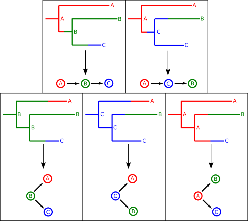
If does indeed describe the ancestral relationships between the isolates collected from the elements of , and we know that we have sampled every host and that there is no reinfection, it is quite intuitively clear (see figure 1) that an element of corresponds to a transmission history for the epidemic. The preimage of under is the set of nodes that make up . Infection events occur along branches of whose start and end nodes are in different elements of . The assumption of no reinfection mandates the connectedness requirement (or there would be multiple introductions to the same host) and the assumption that all hosts in the outbreak were sampled mandates that each element of contains a tip (because one that did not would correspond to an unsampled host).
To formalise the correspondence, we construct a map such that if and ,
Proposition 3.1.
For , the directed graph given by drawing an edge from to for all is a tree, and if is the root of , the directionality coincides with that given by taking to be its root.
Proof.
For the first part, we must show that the graph is simple, connected, and has no cycles. For simplicity, the construction will never give a node with indegree greater than 1, so if two edges join the same two nodes then their directionality is different. Suppose are such that and . Now and (which may not be distinct) are nodes of , and as a descendant of is also a descendant of in . Similarly, is a descendant of . This contradicts the fact that , as a tree, has no cycles, or, if and , that it is simple.
For connectedness, again suppose and let ; the root of is the root of . It may be that . If not, the path in from to passes through elements of whose elements map under to the hosts , where is some permutation of with and . In particular it must pass through the root nodes of all these subtrees, , implying that for all . It follows that ; thus all hosts in are connected to and each other.
Suppose has a cycle. It must be a directed cycle or else has a node with indegree greater than 1. With denoting a permutation of as before, suppose the cycle has (if then the graph is not simple) elements such that for all and . If , the is a subtree of containing a root node and the parent of the root node of the subtree ; similarly contains . Since for each contains a sequence of nodes, following the directedness of induced by its root, running from to to and there is a directed link from each to in , the concatenation of all of these forms a cycle in , contradicting the fact it is a tree.
For the second part, there is no node by construction, and we have already shown that our construction produces a directed path from each to . As we have shown is a tree, this is the only such path, hence the directedness of all edges is towards . ∎
Proposition 3.2.
is injective.
Proof.
We suppose the we have two partitions that have the same image under , i.e. for all , . If then there exists some node of that has . We can assume that either is the root of or for the parent of (or else we move down to find a new for which this is true).
If is the root of , then it is the root of the subtrees and . This implies but because ; only one element of can be sent to by since the root of is unique. So exists.
Let . First suppose and . Then . We show that is not possible. Let . Now is a descendant of because is the root node of the subtree , and includes . gives rise to another subtree of , , all of whose nodes map to under . This has a root node which is not because . It must, in fact, also be a descendant of ; if it were not, would be disconnected by . The parent cannot have because either a) and by construction or b) and if were true, the subtree of nodes that map to under would be disconnected by . Hence .
So without loss of generality suppose but . Again . Let be the unique tip of that has . Now, is not a descendant of . If it were, then , the subtree of whose nodes are mapped to by , would be disconnected by , which maps to . This implies that there is a descendant of in , possibly itself, which maps to under but neither of whose children and do. (If this were not true, a second tip would map to under ). Whether it is or not, cannot map to under ; if it is then it does not by construction, and if is not, it would have an ancestor, , which did not, and an earlier ancestor, , which did, breaking connectedness. This implies that but .
∎
For the next proposition, we need the following:
Lemma 3.3.
If and is a transmission tree in which is an ancestor of , then if with and is a node of with , has an ancestor in with .
Proof.
Strong induction on the number of intervening hosts between and in . If , this is true by definition of , as the node is an ancestor of and its parent maps to . If the lemma is true for all and the set of intervening hosts has size , let be an arbitrary member of that set. The number of intervening hosts between and in is less than , so has an ancestor in with . The number of intervening hosts between and in is also less than , so has an ancestor in with . It follows that is the ancestor of that we need. ∎
Proposition 3.4.
is not surjective for .
Proof.
For , and since the latter is simply the number of assignments for the single internal node of to a subgraph containing one tip or the other. The map’s injectiveness ensures its surjectiveness. If , then let be any three hosts. In , , and have a most recent common ancestral node and two of them, without loss of generality and , have a most recent common ancestral node which is a descendant of . We show that there is no element of which will map to any member of in which any of the following are true:
-
•
is an ancestor of , which is an ancestor of .
-
•
is an ancestor of , which is an ancestor of .
-
•
is an ancestor of , which is an ancestor of .
-
•
is an ancestor of , which is an ancestor of .
Let be a partition such that is a transmission tree in which is an ancestor of both and . Now . To see this, note that since is an ancestor of , if it does not map to under then neither do any of its ancestors, by connectedness. Nor do any descendants of the child of which is not an ancestor of and , a set which includes . All ancestors of apart from belong to one of those categories. But this contradicts lemma 3.3 because has no ancestor which maps to under despite the fact that is an ancestor of .
Now has no ancestor in that maps to under , because the node breaks connectedness between and any position that such a node could be. The contrapositive of lemma 3.3 then says that is not an ancestor of . Similarly is not an ancestor of . Likewise, if is such that is an ancestor of both and , is not an ancestor of nor vice versa.
∎
Let the image of under be . The actual cardinality of varies with the topology of , which can be clearly seen in the case (figure 2).
Proposition 3.2 states that no two partitions of the internal nodes of correspond to the same transmission history; the set of partitions and the set of compatible transmission trees are equivalent. Proposition 3.4 shows, however, that not every possible transmission tree on actually corresponds to a partition of the nodes of a fixed . If we are interested in exploring the complete space of transmission trees using this construction, we need to vary the phylogeny as well.
Let the set consist of all partitions of all phylogenies with tips labelled with . The map can be extended to a map in the obvious way.
Proposition 3.5.
is surjective. In other words, any transmission tree on arises as a partition of some phylogenetic tree .
Proof.
Let . Use the following procedure to construct an element of . If each has children in , take nodes . Pick an arbitrary ordering of the children of each and make a graph by drawing two edges from each to and from to where is such that is the th child of in the ordering. (Notice that gets no children either way.) If is such that is the root of , let the root of be .
It is clear that is a rooted binary tree, its tips are the and if each of these is labelled with the corresponding then they are in one-to-one correspondence with . The set of nodes for each are by construction connected in and contain the single tip ; hence this partitioning of the nodes of is an element of . It is easily checked that . ∎
As an aside, is not injective, as is clear from the arbitrary choice of ordering for the children of each . (In fact, some elements of cannot be produced by this construction at all, for example, the bottom right example in figure 1.) The upshot of proposition 3.5 is that a MCMC procedure that fully explores the space of these partitioned phylogenies is also fully exploring the space of transmission trees amongst the elements of . We outline such a procedure in the next section.
So far, we have only dealt with the phylogenetic tree topology . If this construction is to be useful for epidemic reconstruction, we must now consider branch lengths. Let be a partition of , and suppose is the topology of a genealogy with length function and height function . Suppose and that . Let , and let be the parent of . An infection event occurs on the branch between and , which means, assuming that internal nodes of and transmissions do not occur at exactly the same time, that it occurs at a height in the interval . In what follows it will be convenient to use a forwards timescale, so let be a function converting between tree height and such a timescale (in the same units, so branch lengths are maintained). Let be this time of infection in forwards time. Let be such that . If , i.e. is the first host in the epidemic, then is between ( being the root node of ) and (remembering that we gave a finite branch length) we can similarly define such that .
The combination of a genealogy , partition and a set of s for all elements then entirely determines the transmission history of the epidemic, describing which host infected which others and when. No assumptions are made at this, conceptual, stage about when hosts cease to be infectious; a host can continue to infect others at any time following the time at which is sample was acquired. If, as will often be the case, this is an unreasonable assumption, the likelihood of such partitions can be evaluated to zero in the calculation of the posterior probability.
4 MCMC procedure
The most common methods for estimation of time-resolved phylogenies involve the use of Bayesian MCMC to sample from the probability distribution of phylogenetic trees given the available sequence data. The previous section demonstrates that, if the sequence data is such that one sample is taken from each host, such procedures can be extended to simultaneously sample from the probability distribution of reconstructed epidemics each sampled tree is augmented a partition of its nodes as well as the values of each . We have implemented this procedure in the package BEAST [12]. Because of the special requirements of this type of augmentation, the standard moves on the phylogenetic tree topology cannot be used. Nor are the structured tree operators developed by Vaughan et al. [13] suitable, as those are designed for the exploration of the space of trees where every point on every branch can be freely assigned a “type” from a finite set. This condition is much less restrictive than than connectedness requirements that we have outlined above and the result of such a move on a tree of our type would not necessarily meet our requirements for partitions. Instead, specialised moves have been devised to alter the partitioned phylogeny in such a way that the transmission tree structure is maintained. In addition, we give an operator to alter the transmission tree while keeping the phylogenetic tree fixed, by changing node labels.
Note that these moves do not simultaneously change the value of any of the s, as moves on these are proposed and evaluated separately. Nevertheless, changes to either tree may involve resampling the times of infection of some hosts. If , changing partition from to may mean that and are different nodes with different heights, and so while will not change, will. Even a move has no effect on the partition or phylogenetic tree topology, such as a change to branch lengths, may also alter the height of and/or its parent, which will also modify while remains fixed.
Definition 4.1.
For a partition of a phylogeny , if is a phylogenetic tree node with we say is ancestral under if it is an ancestor of the only member of the subtree which is a tip of .
Definition 4.2.
For a partition of a phylogeny , the infection branch for is the branch of ending in .
4.1 Infection branch operator
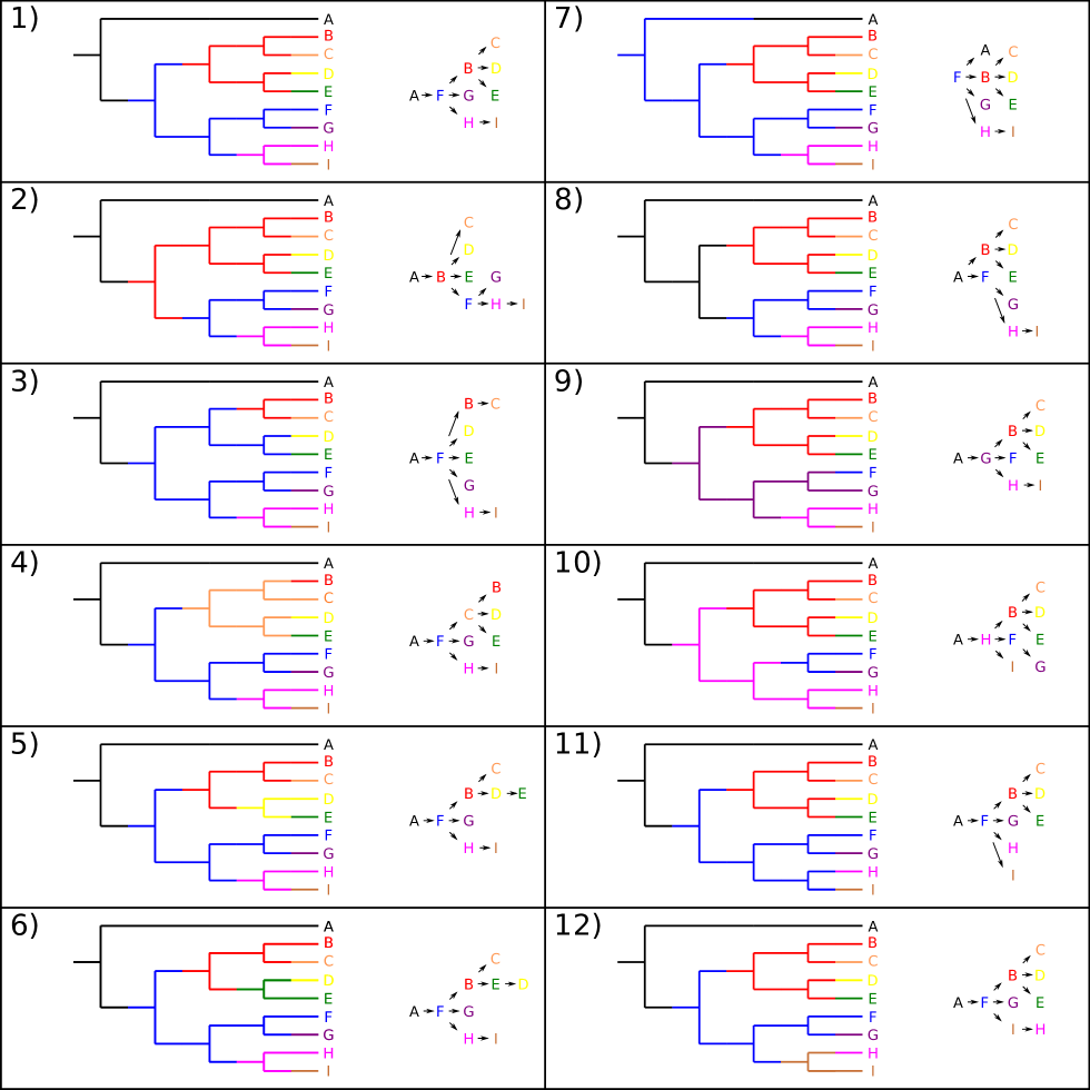
We randomly select a host that is not the first host in the outbreak (i.e. is not the root of ). Consider . The operator performs both “downward” and “upward” moves, but if is a tip then the move must be downwards. If it is internal, then we select upwards or downwards each with probability 0.5. Let and be the parent of (which must exist as we avoided the root). It must be that and are in different elements of , and this implies that is ancestral under because the path from any node that is not a descendant of to must pass through and if this would violate the connectedness requirement. Suppose .
Upward move
We create a new partition that has , moving the infection branch of up the tree. Consider the two children and of (as this is the upward move, is not a tip). At least one of these is mapped to the same element of as by because must be in the same element of as the tip and the path from to this tip in the subtree will intersect one of its children. If this is true of only one child then without loss of generality say it is . In this case we can simply make by setting and leaving the rest of the partition unchanged; this is clearly still a valid partition because all subtrees remain connected. So suppose also . At most one of and is ancestral under (as siblings, they cannot both be ancestors of the same tip) so, again without loss of generality, say it is . If we again set , the removal of from the subtree splits the nodes of the latter into two sets, containing and , and containing . The nodes of both sets and the edges between them form connected subtrees of , but their union is not connected. We complete the construction of by setting for all . and are then connected.
The effect on the transmission tree is that all that have and a descendant of have instead.
Downward move
We create a new partition that has , moving the infection branch of down the tree. We need to consider the grandparent of if it exists, and the child of that is not . At least one of and must be in the same element of as (or else is not in a partition element containing a tip). If does not exist then this must be .
If and either or does not exist, then setting is all that is required to make a valid partition. The two or three nodes joined to by edges were all in different elements of and remain so; was in the element of containing one of its children and is moved to the one containing the other child in . Similarly, if and , then then all we need do is set ; the situation is the same except that the has moved from the element of that contains of one of its children to the one containing its parent.
If exists and , then the removal of from the subtree splits into two subtrees whose union is again not a connected subtree of . Let the node sets of these two subtrees be and , with containing and containing . If is ancestral under then also contains the tip , and if it is not then does. We complete by setting for all in the set that does not contain . and are now connected. Note that may contain the root node and if it does not contain then the root’s image under is different from that under , which is how this move may change the first host in the outbreak even though the root host is never chosen by the move. This can be seen in example 7) of figure 3.
If is not ancestral under , then the effect on the transmission tree is that all that have and a descendant of have instead. If is ancestral under then, in , is the infector of instead of vice versa, and all that have and not a descendant of have instead.
Hastings ratio
We observe that:
-
•
The upward move on is reversed by the downward move on the child of that is ancestral under . Thus the Hastings ratio is 1 if is not a tip and 2 if it is.
-
•
If is not ancestral under , then the downward move on is reversed by the upward move on . The Hastings ratio is 1 if is not a tip and if it is.
-
•
If is ancestral under , then the downward move on is reversed by the downward move on its sibling . The Hastings ratio is 1 if and are both tips or both not tips, 1/2 if is but is not, and 2 if is but is not.
The various variations of this move are depicted in figure 3. If the initial partition is that depicted as 1), the downward moves depicted as 2), 4), 7), 9), 10) and 12) involve a parent that is ancestral under and 5) and 6) involve one that is not.
4.2 Phylogenetic tree operators
We have adapted the three standard tree moves used in BEAST (exchange, subtree slide, and Wilson-Balding [14, 15, 16]) such that they respect the transmission tree structure induced by partitioning the internal nodes. We give two versions of each:
-
•
A “type A” operator which does not alter the transmission tree at all; all parental relationships remain the same.
-
•
A “type B” operator which performs phylogenetic tree modifications which simultaneously rearrange the transmission tree by assigning new parents to one or two hosts.
4.2.1 Type A operators
Type A exchange
Select a random node that is not the root of the phylogenetic tree , and then randomly selects a second node , also not and not the sibling of , such that the parents and of and are in the same element of , , and . If there is no such then the operator fails. Otherwise, and exchange parents to obtain a new phylogenetic tree with the same partition of nodes . is still valid in terms of connectedness, because if then all nodes in the element of containing are descendants of and the move has not affected them, whereas if then changing ’s parent to means that after the move it is still adjacent to a node with the same image under as itself; the same goes for . The transmission tree structure is unchanged: if then is infected by before the move and is by afterwards, whereas if then ’s infection branch was not affected at all. Again, the same goes for .
For the Hastings ratio, note that the partitioned tree obtained by selecting and then is exactly the same as that obtained by selecting and then . If a node is selected first, let be the number of eligible nodes to be selected as the second (this is explicitly calculated every time the operator acts). The denominator of the Hastings ratio is then . The move is reversed by selecting the same two nodes again (in either order) hence we calculate and and the ratio’s numerator is . Cancellation gives .
Type A subtree slide
Select a random node under the conditions that and either ’s grandparent or sibling (or both) is in the same element of as its parent . Draw a distance from some probability distribution that is symmetric about 0. We aim to change the height of to . If , examine ’s ancestors to find a node such that either or but ; if no such ancestor exists then let and this is true. If then the move fails. If then simply change the height of to and the topology is unchanged. Otherwise, modify the tree such that has height , parent (or no parent if in which case is now the root node) and child , and has parent . Again, do not change . Connectedness rules are still obeyed because, in the new tree , is adjacent to , which is in the same element of as itself. The transmission tree structure is unchanged as:
-
•
The move does not change the partition, so any infection branches have not changed if the particular phylogenetic tree branch was not modified by the move. This applies to the branch between and as well as all branches adjacent to nodes other than , , , , , and .
-
•
If and are in different elements of then and are in the same one, so the infector of remains the same.
-
•
If and are in different elements of then the move fails if so the phylogenetic tree topology is unchanged.
-
•
If and are in different elements of then , instead of , is now the end of ’s infection branch, but and its infector is still .
If , then if the move fails. Otherwise, we select a node at random from the set which consists of nodes that:
-
1.
Are descendants of but not descendants of .
-
2.
Have but .
-
3.
Have .
If is empty the move fails. In the case that consists only of then simply set and the topology is unchanged. Otherwise, modify the tree such that has height , parent and child , and has parent . connectedness rules are still obeyed because there is an edge from to a node () in the same element of the partition. The transmission tree structure is unchanged as:
-
•
Again, the move does not change the partition, so any infection branches have not changed if the particular phylogenetic tree branch was not modified by the move.
-
•
If and are in different elements of then the move fails if so the topology is unchanged.
-
•
If and are in different elements of then and were in the same one, so the infector of remains the same; is now the end of its infection branch.
-
•
If and are in different elements of then the infector of is still .
Suppose there are nodes eligible for this move before it occurs and afterwards. If the topology did not change then the Hastings ratio is . Otherwise, it is if and if , where the is the set of nodes that:
-
1.
Are descendants of (in the original tree) but not descendants of .
-
2.
Have but .
-
3.
Have .
Type A Wilson-Balding move
Pick a node under the same conditions as for the type A subtree slide. Pick a second node at random from amongst all nodes that are in the same element of as , or whose parents are, and such that . The move fails if , or . The node is pruned and reattached as a child of and the parent of as with the standard Wilson-Balding move [14, 15]. As before, do not change . Connectedness rules are obeyed because there is an edge from to a node (either or ) in the same element of as itself. The transmission tree structure is unchanged because if there was an infection event between and (and there was at most one by construction) then there still is and it involves the same hosts, and likewise if there was one between and then there still is and it involves the same hosts. If there was no infection event in either case then the removal or insertion of does not add one.
Notice that if is subsequently selected for this move again, then the set of candidates for the second node is the same except that it excludes the original and includes the original ; in particular it has the same cardinality, as it did for the standard Wilson-Balding move. So only the choice of first node affects the Hastings ratio. It follows that this is the ratio from the standard Wilson-Balding move multiplied by , where is the number of nodes eligible for this move before it occurs and is the number afterwards.
4.2.2 Type B operators
Type B exchange
Select a random node , not , whose parent is in a different element of to itself. Pick a second node , also not and not , whose parent is also in a different element of to itself (but this time the elements containing and do not have to be the same), such that , and . If there is no such then the operator fails. Otherwise, and exchange parents as with the type A operator. That it preserves connectedness of subtrees is clear. The effect on the transmission tree is that and exchange parents (if their parents are different).
The Hastings ratio is calculated in effectively the same way as for the type A version, noting that the number of choices for is just . If is the number of eligible choices for a second node if is chosen first, then the ratio is .
Type B subtree slide
This time, is a random node whose parent exists and is in a different element of to itself. This implies that is in the same element as either or (if the latter exists) because otherwise would not be in a partition element containing a tip. The operator performs the standard subtree slide move [16] on , inserting as the parent of another node and (if was not the root node), the child of . is changed to a new partition as follows: if does not exist or and are in the same element of , is moved to the element containing . Otherwise, it is moved to either the element containing or that containing with equal probability. This reallocation is enough to ensure that obeys connectedness rules. The effect on the transmission tree is that is moved to become a child of either or . If then was the child of before the move and remains so.
Noting that there are always choices for , the Hastings ratio is the same as the standard subtree slide move, except that the denominator is multiplied by if exists and and are not in the same element of , and the numerator is multiplied by if exists and and are not in the same element of .
Type B Wilson-Balding move
In a similar way, is randomly picked from the set of nodes whose parents exist and are in different subtrees to themselves, and the standard Wilson-Balding move is performed on it, inserting as a parent of another node and a child of its parent if that exists. The reassignment of to a new subtree is performed in the same was as for type B subtree slide, and the adjustment to the Hastings ratio is identical. The effect on the transmission tree is also the same.
4.3 Irreducibility of the chain
Suppose is a partition of a phylogeny with root node . First, notice the following about the infection branch operator described above:
-
•
For any , if , a series of downward moves, starting with one on , eventually results in a new partition which has .
-
•
If , a series of upward moves on for all will eventually give a partition in which for all internal nodes of . As all such moves are reversible, we can get from to any partition that has .
The above demonstrates that a MCMC chain made up of these moves on the space of partitions of a single phylogeny is irreducible. If and are two partitions such that then there is a series of moves taking to , and if then there is a series of moves taking to a partition that has and then a series of moves taking to .
To extend this to a variable phylogenetic tree, we use the fact that in the space of standard, unpartitioned phylogenies, the Wilson-Balding move on its own is sufficient for irreducibility [15]. Suppose is a partition of such that for all internal nodes of . Now every node of is eligible to be the first node chosen by the type A Wilson-Balding move, as is true with the standard Wilson-Balding move on an unpartitioned tree, and subsequently, the set of nodes that is eligible to the the second node chosen is the same for both moves too. In addition, after this move, the new tree is still partitioned such that all internal nodes are in the same element of the partition. As a result, every move on an unpartitioned phylogeny that can be made by the standard move is also possible on the space of partitioned phylogenies with all internal nodes in the same partition element as a unique tip. Hence the chain is irreducible under the type A move when restricted to phylogenies with partitions of this type, and we have already shown that the infection branch operator is sufficient to move from a partition of this type to any other partition of the same tree. This is sufficient to establish irreducibility on the entire space of partitioned phylogenies using just these two moves.
5 Bayesian decomposition
Having established the correspondence between partitioned phylogenetic trees and transmission trees, we now show how the likelihood of such a partitioned phylogeny can be calculated given models of between-host transmission dynamics, of the duration of the infection within each host, of the population dynamics of the “agents” (which can be taken to be pathogens or infected individuals) within each host, and of sequence evolution.
In contrast to the previous work of Didelot et al. [8], whose underlying model of transmission was a compartmental SIR model, we use an individual-based model similar to those employed in previous work on agricultural outbreaks [1, 5, 3, 6]. This much more readily allows for the accommodation of host heterogeneity, and makes no assumption of random mixing. Instead, the force of infection of a host on another is given by a basic transmission rate multiplied by a positive real number from a function describing some relationship between and . Possible choices for are a spatial kernel function, a network metric, or a function modifying based on shared membership in some class of host.
As in previous work [6, 8] we take the model of the dynamics of the “agents” to be a coalescent process amongst lineages in a freely-mixing population within each host. If the hosts are single organisms, the agents will naturally be individual pathogens. If, on the other hand, the hosts are infected locations, they could instead be considered to be infected organisms. In either case, only a miniscule proportion of the total agent population are represented by lineages in the tree, and the assumption of a low sampling fraction required for use of the coalescent process is satisfied.
We use the following notation:
-
•
The sequence data,
-
•
The phylogenetic tree,
-
•
The transmission tree structure,
-
•
The set of times of infection of each host
-
•
The times of sampling of the sequence from each host
-
•
The times of becoming noninfectious of each host.
-
•
Data describing the relationship between hosts that is used to define the function (for example, spatial locations).
-
•
The basic transmission rate .
-
•
The parameters of the distance function .
-
•
The parameters of the population dynamics of the agents within each host.
-
•
The parameters of the nucleotide substitution model and molecular clock.
We condition on , , and . We assume that and are not contradictory; no sample was taken after a host became noninfectious. can be the same set of times as , or a separate set of later times. If any or all hosts are known to have remained infectious indefinitely, their values of can be set to the time at which the last sample was taken.
The posterior probability we are interested in calculating is . By Bayes’ Theorem this is equal to:
As usual, we need not calculate the denominator if we are uninterested in model comparison as it does not vary. We assume that mutations occur neutrally over the the phylogenetic tree in a process that ignores the host structure, so depends only on and and the likelihood reduces to , which can be calculated using the Felsenstein pruning algorithm and a molecular clock model in the normal way [17, 15, 18]. It remains to calculate the prior probability . The full decomposition is as follows:
The following assumptions of independence are then made:
-
•
All parameters in the decomposition are independent of .
-
•
, the base transmission rate, is (at least) conditionally independent of and given , , , , , and . This is intuitive given that the latter set of parameters completely describe the epidemic and the distance-based modification of .
-
•
, the phylogenetic tree, is (at least) conditionally independent of , , and given , , , and .
-
•
, the transmission tree structure, is (at least) conditionally independent of and given , , and .
-
•
, the times of infection, is (at least) conditionally independent of , , and given .
-
•
, and are independent of , , , and each other.
The decomposition then reduces to:
For calculation of , we use Bayes’ Theorem again:
The denominator can be evaluated as
by the law of total probability. This will not in general have a closed form solution and we use numerical integration to estimate it. The term is our prior belief in the value of given and the background information; in the absence of other information we take to be independent of these and simply give it any prior distribution that we please.
It remains to calculate . The calculation here is along the same lines of that introduced by Gibson and Austin [19], but heavily modified. Given a particular set of , we reorder the indexes of to be in increasing order of infection. As before, the infection time of is . The probability that was infected at time given that it was first in the epidemic is effectively unknowable and we set it to 1. For notational simplicity now treating as a map from the index of a case to the index of its infector, we need the probability that infected at , which is made up of:
-
•
The probability that infected at , but not before:
-
•
The probability that no other host infected before . As we assume no reinfection, infection events that would occur after this time are ignored. Noting that the last possible time that an could have infected for this to be true is the smaller of and the end of of ’s infectiousness, , this is given by:
-
•
As we are conditioning on and , we implicitly assume that each was, in fact, infected and was infected before its time of sampling . As a result, we need to normalise by the probability that an infection did happen before this date, which is one minus the probability that none did. The last possible time that an could have infected at all is the smaller of and , so this expression is:
Thus the full expression for is:
If one of the terms in this expression is zero, then the whole thing is zero, representing an impossible transmission history. Otherwise this is undefined for but exists and is positive for all other , as the denominator is always greater than zero. Let this expression, as a function of alone with all other variables constant, be . The integral , where is the prior probability of , can estimated by numerical methods if we show that it is in fact finite.
Proposition 5.1.
Let . The improper integral converges as and .
Proof.
For the lower limit, we use:
Lemma 5.2.
Suppose and are positive real numbers. Then:
Proof.
Let and . Then and . Hence:
This shows that and the result follows by l’Hôpital’s rule.
∎
Lemma 5.2 shows that each individual term in the product that makes up does not have 0 as an asymptote, hence they are all bounded on as they clearly have no others. Hence, on this interval, , as the product of bounded functions, is bounded and the integral converges.
For the upper limit, we can write:
where , and each is a positive real number. If we let then whose limit as is 1. The limit comparison test then says that converges as if and only if does. Recursive integration by parts gives:
, and can thus be expressed as a constant expression involving , plus the sum of limits of the form where is a constant and . It is a standard result that each of these is 0. Hence converges and so does .
∎
Corollary 5.3.
Let . If is a proper prior distribution whose support is a subset of , the improper integral converges as and .
Proof.
If has finite support, then is bounded on a finite interval and zero elsewhere, and the intergral of such a function must converge. If not, then use of the limit comparison test with numerator and denominator gives that, because , converges if does, and we know this to be true. ∎
Remark 5.4.
Notice that if is, for example a uniform infinite improper prior or a gamma distribution, takes the form for a function where and are positive constants and . Generalised Gauss-Laguerre quadrature is therefore a natural choice for the estimation of for such a .
Next, we need to calculate . We extend the procedure outlined by Didelot et al[8] to allow for the use of any of the standard models of deterministic population growth, and the possibility of host heterogeneity. The latter is accomplished by dividing the set of hosts into categories and assigning a separate demographic model to all the hosts in each one. Categories can be assigned from known epidemiological data about the hosts; for example, in a livestock disease outbreak, they may reflect the size of farm. Formally, let , a finite set of size , be the set of categories, and the map assigning them to the index of each host in . If it is not desired to accommodate heterogeneity in this way, can be 1. Every element corresponds to a separate demographic function with parameters where is the product of the effective population size and the generation time at time .
Given a host which is infected at time , sampled at time and ceases to be infectious at time , and has children (for some permutation of ) infected at times , suppose is a phylogenetic tree that describes the part of the outbreak that took place within . It has has tips, one for each infection event and one for its own sampling event. If , the height (in the tree ) of its root node is less than and we can give it a root branch of length . If we have a for each , and we know , we can build a phylogenetic tree for the entire epidemic by attaching the root node of each to the tip of that corresponds to the infection of , by a branch with length equal to the root branch length of . If cannot be built up from s in this way, . Otherwise, we calculate it as:
In the standard coalescent model [20], the probability density function for the for the time of the first coalescence of lineages after where the demographic function is is given by:
and as usual, if we know the two specific lineages that converged, the cancels.
The cumulative density function of this is:
and the probability that there were no coalescences between and is 1 minus this.
As Didelot et al. [8] note, this is not quite sufficient for our purposes because we have a maximum height for the last coalescence. If this is , the normalised probability distribution for the time of first coalescence is:
This is the probability of an interval in ending in a coalescent event. The probability of an interval ending in a transmission or sampling event is the probability that no events occur in the interval, which is one minus the cumulative distribution function of the above, :
Note that while in the case of no maximum root height, the formula happens to work for , here it does not as the denominator is 0, and we instead set the probability of any coalescent interval with one lineage to 1. In particular, if has no children then .
If , these formulae can be used to calculate for every in the established way for a tree with temporally offset tips [15], and the product of these is the full probability of the complete phylogeny. It is most intuitive to standardise the timescale within each such that the effective population size at the point of the infection (the maximum root height) is the same across all hosts. As a result, we depart from the normal convention of making height 0 the time of the last tip (which will occur at a different point in the course of infection in different hosts), and instead put it at the point of infection, with all later events occurring at negative heights.
The choice of each demographic function is wide. For an epidemic situation, exponential or logistic growth [20, 21] would be most appropriate. Different categories may be assigned the same family of demographic model but a different set of parameters . As our method is integrated within BEAST, any of the functions already implemented in that package can be used without additional programming work.
The next term in the decomposition is . The instantaneous probability that host was infected by host at time is , and if we condition on the fact that was indeed infected by some host at then we normalise by the sum where is the subset of whose elements have infection times before and noninfectiousness times after it. In this normalisation the s cancel, leaving an expression solely in terms of the distance function. The probability of the infection of the first host is once again set to 1. The expression is:
There are many possible choices for the function . If we assume no spatial structure or heterogeneity then we can just take for all . Otherwise, it can be based on Euclidean distance, or on a network metric. It can also be used to state prior information about the transmission tree structure; if it is known a priori that did not infect , then can be set to zero. While we have assumed it up to this point, there is also no requirement that be symmetric.
The calculation of , the probability of the times of infection, can be handled in a number of ways. It is effectively the calculation of the probability of the time from infection to noninfectiousness, , of each host . Previous work on foot-and-mouth disease virus [1, 5] has used clinical data to estimate times of infection, and if this kind of information is available, it can be used to determine a separate prior distribution for each . If we cannot use information of this type, we take a similar approach to that in the coalescent calculations above and assign each host to a category from a finite set of size . This again allows us to accommodate known host heterogeneity; for example in an agricultural outbreak it is likely that times from infection to noninfectiousness decrease as time goes by and control measures are brought to bear. Once again, if we do not want to incorporate such heterogeneity we can set . If the infectious period of the disease is well understood, we can assign a single prior distribution for for all hosts in each category.
It may be, however, that we want to estimate the distribution of infectious periods from the genetic data. In this case we take each within a category as a draw from a probability distribution with unknown parameters, and then put hyperpriors on those parameters. A noninformative option is to regard each as a draw from an unknown normal distribution whose mean we are uninterested in (as we can just as well calculate the mean of the sampled values of each infectious period post-hoc) and use the Jeffreys prior on its standard deviation, such that is proportional to the reciprocal of the standard deviation of all the infectious periods in the category. This can obviously be done on the logarithm of the infectious periods instead, if we prefer the assumption that they are lognormally distributed. Alternatively, we can use an informative prior. To avoid having to use MCMC to estimate both the parameters of a probability distribution and a series of draws from that distribution, we integrate out the actual values of by using ’s conjugate prior for them and then calculating the marginal likelihood of the infectious periods given the hyperpriors. Any continuous probability distribution with a prior whose marginal likelihood is analytically tractable can be considered. A normal distribution is not absolutely ideal as infectious periods are non-negative parameters, but it does have the useful property that its mean and variance are independent, unlike most other candidates for (such as lognormal, exponential or gamma). We suggest it still be considered as an option if infectious periods are expected to be sufficiently long, and their variance sufficiently small, that the probability density contained in the area less than 0 would negligible if a normal distribution were used.
Finally, all that remains is to place prior distributions on the parameters making up , , and .
Latent periods
The above formulation has taken the course of infection to follow a SIR structure; hosts are assumed to be infectious as soon as they are infected. It is straightforward to replace this with a SEIR structure instead. We add an extra set of parameters consisting of the time of infectiousness of each host . In the MCMC procedure these are calculated by adding a such that, if ( being the upper bound on determined by and ), then . (We assume that hosts are infectious at the time they cease to be infected, but not that they necessarily are at the time of sampling.) Simple MCMC moves on numerical parameters are then employed to sample values of each . The phylogeny is assumed to be conditionally independent of given .
The decomposition becomes:
The only modifications to the existing procedure that are needed to calculate the first and third elements in this product involve accounting for the fact that infectious pressure is now only applied after the end of a host’s latent period. The term is calculated by retaining the existing procedure for infectious periods and also picking a suitable distribution, or possibly set of distributions according to a set of categories, for latent periods. The marginal likelihood of the set of infectious periods and latent periods is then calculated as before.
6 Conclusions and future work
The most obvious limitation to the method outlined here is the requirement that the tree contain a tip from every host involved in the outbreak. Note that this is not, in fact, a requirement that a sequence be taken from every host, as, if we have no sample from some but are aware of their existence, we can use epidemiological data for them along with a noninformative sequence (consisting entirely of the nucleotide code ‘N’) and integrate over their unknown true sequences. Their existence would then still contribute to estimation of epidemiological parameters, and their estimated placement in the transmission tree would be informed by their geographical locations if those were included in the model. The performance of this procedure for varying numbers of unknown sequences warrants investigation in simulations. Nevertheless, this is a solution only where all unsampled hosts are actually known to investigators, which will not always be the case. Non-phylogenetic methods for transmission tree reconstruction using genetic data have started to consider the case of unsampled hosts [7, 9] and work is needed to introduce this element to our framework. This could be done by introducing a variable number of partitions containing no tips, possibly in a reversable-jump MCMC framework, or by simply assigning tree nodes to “nonsampled” subtrees with no specific enumeration of how many extra hosts these represent.
Another enhancement, potentially useful in HIV studies where multiple samples are taken from the same patient over time, would be to relax the partition rules to allow each subtree to contain more than one tip. The adjustments to the method needed to accomplish this are likely considerably less onerous than allowing for unsampled hosts.
In conclusion, in this document we have outlined the framework for co-estimation of transmission trees as part of an analysis performed in one of the most widely-used software packages for phylogeny reconstruction. Results from analyses of both simulated and real data will follow. It is, as of the time of writing, implemented in current development builds of BEAST.
7 Acknowledgements
We would like to thank Trevor Bedford, Samantha Lycett and Melissa Ward for contributions to the development of this model. MH was supported by a PhD studentship from the Scottish Government-funded EPIC programme, and the research leading to these results has received funding from the European Union Seventh Framework Programme for research, technological development and demonstration under Grant Agreement no. 278433-PREDEMICS
References
- [1] Cottam EM, Thébaud G, Wadsworth J, Gloster J, Mansley L, et al. (2008) Integrating genetic and epidemiological data to determine transmission pathways of foot-and-mouth disease virus. Proceedings of the Royal Society B: Biological Sciences 275: 887-895.
- [2] Aldrin M, Lyngstad TM, Kristoffersen AB, Storvik B, Borgan Ø, et al. (2011) Modelling the spread of infectious salmon anaemia among salmon farms based on seaway distances between farms and genetic relationships between infectious salmon anaemia virus isolates. Journal of The Royal Society Interface 8: 1346-1356.
- [3] Ypma RJF, Bataille AMA, Stegeman A, Koch G, Wallinga J, et al. (2011) Unravelling transmission trees of infectious diseases by combining genetic and epidemiological data. Proceedings of the Royal Society B: Biological Sciences 279: 444-450.
- [4] Jombart T, Eggo RM, Dodd PJ, Balloux F (2011) Reconstructing disease outbreaks from genetic data: a graph approach. Heredity 106: 383-390.
- [5] Morelli MJ, Thébaud G, Chadœuf J, King DP, Haydon DT, et al. (2012) A bayesian inference framework to reconstruct transmission trees using epidemiological and genetic data. PLoS Computational Biology 8: e1002768.
- [6] Ypma RJF, Ballegooijen WMv, Wallinga J (2013) Relating phylogenetic trees to transmission trees of infectious disease outbreaks. Genetics 195: 1055-1062.
- [7] Jombart T, Cori A, Didelot X, Cauchemez S, Fraser C, et al. (2014) Bayesian reconstruction of disease outbreaks by combining epidemiologic and genomic data. PLoS Computational Biology 10: e1003457.
- [8] Didelot X, Gardy J, Colijn C (2014) Bayesian inference of infectious disease transmission from whole genome sequence data. Molecular Biology and Evolution .
- [9] Mollentze N, Nel LH, Townsend S, Roux Kl, Hampson K, et al. (2014) A bayesian approach for inferring the dynamics of partially observed endemic infectious diseases from space-time-genetic data. Proceedings of the Royal Society B: Biological Sciences 281: 20133251.
- [10] Vrancken B, Rambaut A, Suchard MA, Drummond A, Baele G, et al. (2014) The genealogical population dynamics of HIV-1 in a large transmission chain: bridging within and among host evolutionary rates. PLoS Computational Biology 10: e1003505.
- [11] Bataille A, van der Meer F, Stegeman A, Koch G (2011) Evolutionary analysis of inter-farm transmission dynamics in a highly pathogenic avian influenza epidemic. PLoS Pathogens 7: e1002094.
- [12] Drummond AJ, Suchard MA, Xie D, Rambaut A (2012) Bayesian phylogenetics with BEAUti and the BEAST 1.7. Molecular Biology and Evolution 29: 1969-1973.
- [13] Vaughan TG, Kühnert D, Popinga A, Welch D, Drummond AJ (2014) Efficient bayesian inference under the structured coalescent. Bioinformatics : btu201.
- [14] Wilson IJ, Balding DJ (1998) Genealogical inference from microsatellite data. Genetics 150: 499-510.
- [15] Drummond AJ, Nicholls GK, Rodrigo AG, Solomon W (2002) Estimating mutation parameters, population history and genealogy simultaneously from temporally spaced sequence data. Genetics 161: 1307 -1320.
- [16] Hohna S, Defoin-Platel M, Drummond A (2008) Clock-constrained tree proposal operators in bayesian phylogenetic inference. In: 8th IEEE International Conference on BioInformatics and BioEngineering, 2008. BIBE 2008. pp. 1-7. doi:10.1109/BIBE.2008.4696663.
- [17] Felsenstein J (1981) Evolutionary trees from DNA sequences: a maximum likelihood approach. Journal of Molecular Evolution 17: 368-376.
- [18] Drummond AJ, Ho SYW, Phillips MJ, Rambaut A (2006) Relaxed phylogenetics and dating with confidence. PLoS Biology 4: e88.
- [19] Gibson GJ, Austin EJ (1996) Fitting and testing spatio-temporal stochastic models with application in plant epidemiology. Plant Pathology 45: 172–184.
- [20] Slatkin M, Hudson RR (1991) Pairwise comparisons of mitochondrial DNA sequences in stable and exponentially growing populations. Genetics 129: 555-562.
- [21] Pybus OG, Charleston MA, Gupta S, Rambaut A, Holmes EC, et al. (2001) The epidemic behavior of the hepatitis C virus. Science 292: 2323-2325.