Crystal-liquid interfacial free energy via thermodynamic integration

Abstract

A novel thermodynamic integration (TI) scheme is presented to compute the crystal-liquid interfacial free energy ($\gamma_{\rm cl}$) from molecular dynamics simulation. The scheme is applied to a Lennard-Jones system. By using extremely short-ranged and impenetrable Gaussian flat walls to confine the liquid and crystal phases, we overcome hysteresis problems of previous TI schemes that stem from the translational movement of the crystal-liquid interface. Our technique is applied to compute $\gamma_{\rm cl}$ for the (100), (110) and (111) orientation of the crystalline phase at three temperatures under coexistence conditions. For one case, namely the (100) interface at the temperature $T=1.0$ (in reduced units), we demonstrate that finite-size scaling in the framework of capillary wave theory can be used to estimate $\gamma_{\rm cl}$ in the thermodynamic limit. Thereby, we show that our TI scheme is not associated with the suppression of capillary wave fluctuations.

I Introduction

The interfacial free energy between a crystal phase in coexistence with its liquid phase, $\gamma_{\rm cl}$, is an important thermodynamic quantity which controls the rate of homogeneous nucleation and the morphology of a crystal growing from its melt turnbull-cech50 ; turnbull50 ; turnbull52 ; woodruff73 ; tiller91 . The magnitude and anisotropy in $\gamma_{\rm cl}$ determines whether crystal growth occurs in a planar, cellular or dendritic manner. Even a small dependence on the orientation of the crystal, e.g., may significantly affect the final microstructure of the growing crystal and the materials properties of the resulting crystal. Moreover, the crystal-liquid interfacial free energy also affects the barrier for the formation of a nucleus near a wall as well as the wetting behavior of the crystal.

In spite of its central importance for a proper understanding of growth and nucleation phenomena, reliable experimental data for $\gamma_{\rm cl}$ is hard to come by. Most experimental studies obtain the crystal-liquid interfacial free energy indirectly by applying classical nucleation theory to homogeneous nucleation rate measurements turnbull-cech50 ; turnbull50 ; woodruff73 ; broughton-gilmer86 ; kelton91 . Such nucleation rate measurements represent an average over the various orientations of the crystal and therefore provide no information regarding the anisotropy of the crystal. Besides, the assumptions inherent in classical nucleation theory affect the estimates of $\gamma_{\rm cl}$. With state-of-the-art experiments, however, $\gamma_{\rm cl}$ can be estimated in certain parameter ranges with an accuracy of 10-20% bokeloh11 ; bokeloh14 ; palberg14 .

In recent years, molecular simulations have emerged as a widely used tool to understand the thermodynamics of crystal-liquid interfaces from a microscopic perspective and obtain reliable estimates of the the crystal-liquid interfacial free energy huitema99 ; tepper-briels2002 ; laird-hamet92 ; davlaird96 ; davlaird98 ; hoyt2001 ; morris2002 ; morris-song2003 ; davidchack2006 ; amini-laird2008 ; zykova2009 ; zykova2010 ; rozas2011 ; hartel2012 ; heinonen2013 ; martin2012 ; finnis2010 ; uberti2011 ; davidchack-laird2000 ; davidchack-laird03 ; laird-davidchack2005prl ; laird-davidchack2005jpcb ; davidchack2010 ; turci2014_1 ; turci2014_2 Currently, several independent simulation techniques are available to determine the crystal-liquid interfacial free energy. In the capillary fluctuation method hoyt2001 ; morris2002 ; morris-song2003 ; davidchack2006 ; amini-laird2008 ; zykova2009 ; zykova2010 ; rozas2011 ; hartel2012 ; heinonen2013 , fluctuations in the height of the crystal-liquid interface are used to compute the interfacial stiffness. Then by using an expansion of the anisotropic interfacial stiffness into cubic harmonics, one can extract, albeit indirectly, $\gamma_{\rm cl}$.

Recently, two related methods to compute $\gamma_{\rm cl}$ have been proposed by Fernández et al. martin2012 and Angioletti-Uberti et al. finnis2010 ; uberti2011 , known as tethered Monte Carlo and metadynamics, respectively. These methods render accurate estimates of $\gamma_{\rm cl}$ with relatively moderate system sizes (less than $10^{4}$ particles). However, both approaches rely on a local order parameter which has been specified only for the (100) orientation of the fcc crystal structure.

In contrast, thermodynamic integration (TI) frenkel-smit02 ; straatsma93 can yield a direct estimate of $\gamma_{\rm cl}$ for various crystal structures, without the necessity of introducing local order parameters and with system sizes of a few thousand atoms. The determination of $\gamma_{\rm cl}$ from thermodynamic integration is based on the definition that the crystal-liquid interfacial free energy is the reversible work required to create a unit area of the crystal-liquid interface adamson97 . Hence, one needs to find a reversible path bringing together independent liquid and crystal phases to create two crystal-liquid interfaces in equilibrium with the bulk phases.

Broughton and Gilmer broughton-gilmer86 first introduced a TI scheme to compute $\gamma_{\rm cl}$ for a modified Lennard-Jones (LJ) potential. Their method consisted of using specially designed “cleaving potentials” to gradually split each phase into two blocks divided by a cleaving plane, then bringing these blocks together, and finally removing the “cleaving potential”. However, designing “cleaving” potentials for various orientations of the crystal, at different coexistence conditions and for different potentials is clearly an arduous task and the “cleaving potentials” proposed by them cannot be easily generalized. Moreover, their calculations were not precise enough to resolve the anisotropy in $\gamma_{\rm cl}$.

Davidchack and Laird davidchack-laird2000 ; davidchack-laird03 ; laird-davidchack2005prl ; laird-davidchack2005jpcb ; davidchack2010 modified the approach of Broughton and Gilmer by using planar “cleaving walls” made of similar particles as the system and consisting of one or more crystalline layers with the same structure as the actual crystal phase. Subsequently, several authors have adopted the “cleaving walls” scheme to compute $\gamma_{\rm cl}$ for various model systems tipeev13 ; wang-apte2013 ; apte2010 . The data reported by them were precise enough to resolve the anisotropy in $\gamma_{\rm cl}$. However, the TI paths corresponding to both the Broughton-Gilmer and Davidchack-Laird approaches are subject to hysteresis in the final step, when the “cleaving walls” or the “cleaving potential” is removed. Due to thermal fluctuations, the two crystal-liquid interfaces can change their position by simultaneous freezing and melting davidchack-laird03 ; davidchack2010 . As a result, their location will no longer coincide with the position of the cleaving plane, leading to hysteresis between the forward and reverse TI paths.

Some authors have tried to adopt the “cleaving walls” TI scheme of Davidchack and Laird davidchack-laird2000 ; davidchack-laird03 into a non-equilibrium work measurement approach musong2006 . Such an approach is independent of the reversibility of the transformation jarzynski1997 ; jarzynski06 . However, the non-equilibrium work measurement still requires one to be able to reach the initial state from the final state when the transformations are carried out in the reverse direction. Due to the movement of the crystal-liquid interface, this is not possible. The hysteresis arising from the mobility of the crystal-liquid interface seems to be a difficult problem to eliminate completely. Though, Davidchack and Laird davidchack-laird03 ; davidchack2010 tried to deal with this issue by performing several independent TI runs and choosing the run with the least hysteresis.

In this work, we propose a novel thermodynamic integration scheme to compute $\gamma_{\rm cl}$ from molecular dynamics simulations. Our scheme circumvents the key problem due to the mobility of the crystal-liquid interface by the use of a very short ranged flat wall (modelled by a Gaussian potential) to split the crystal and liquid phases. Such a short-ranged wall demands that the integration of the equations of motion is carried out with a very small time step. However, this disadvantage can be offset by the use of a multiple time step scheme frenkel-smit02 . The contribution of this short-ranged wall to the final value of the interfacial free energy itself is negligible (much less than the statistical errors and less than $0.1\%$ of the final value of $\gamma_{\rm cl}$). In addition to this short-ranged flat wall, we also insert a structured solid wall consisting of frozen-in crystalline layers, to gradually bring together in a smooth manner the individual crystal and liquid phases split by the flat wall. We employ our thermodynamic integration scheme to compute $\gamma_{\rm cl}$ for a modified Lennard-Jones potential, though our scheme can also be used for more complex potentials.

In order to determine $\gamma_{\rm cl}$ in the thermodynamic limit, we use a careful analysis of finite-size effects in the framework of capillary wave theory binder82 ; schmitz2014 . Although the finite-size effects turn out to be relatively small for systems containing more than about 20000 particles, our finite-size analysis is nicely consistent with the prediction of capillary-wave theory and thus this demonstrates that our TI scheme does not lead to a suppression of capillary-wave fluctuations. This indicates that the Gaussian flat walls introduced in our scheme indeed lead to negligibly small perturbation of the system.

In the next section (Sec. II), we introduce the Lennard-Jones model for which $\gamma_{\rm cl}$ is computed. After describing our TI scheme (Sec. III), the details of the simulation are given in Sec. III.1. The results are presented in Sec. IV, and finally, we end with a conclusion in Sec. V.

II Model

The Lennard-Jones (LJ) potential describes the interaction between a particle $i$ and a particle $j$ separated by a distance $r_{ij}$ and is given by

$$\phi(r_{ij})=4\epsilon\left[\left(\frac{\sigma}{r_{ij}}\right)^{12}-\left(\frac{\sigma}{r_{ij}}\right)^{6}\right],$$ (1)

where the parameters $\epsilon$ and $\sigma$ set the scales for energy and length, respectively. Broughton and Gilmer broughton-gilmer86 proposed a modified LJ potential with a cut-off at $r^{\rm cut}=2.5\,\sigma$ that provides continuity of potential and force at $r=r^{\rm cut}$. It is defined by

$$u(r_{ij})=\phi(r_{ij})+C_{1}$$ (2)

for $0<r_{ij}\leq 2.3\,\sigma$,

$$u(r_{ij})=C_{2}\left(\frac{\sigma}{r_{ij}}\right)^{12}+C_{3}\left(\frac{\sigma}{r_{ij}}\right)^{6}+C_{4}\left(\frac{r_{ij}}{\sigma}\right)^{2}+C_{5}$$ (3)

for $2.3\,\sigma<r_{ij}<r^{\rm cut}=2.5\,\sigma$ and $u(r_{ij})=0$ for $r_{ij}\geq r^{\rm cut}$. The constants in Eqs. (2) and (3) are given by $C_{1}=0.016132\,\epsilon$, $C_{2}=3136.6\,\epsilon$, $C_{3}=-68.069\,\epsilon$, $C_{4}=-0.083312\,\epsilon$, and $C_{5}=0.74689\,\epsilon$.

III Thermodynamic Integration Scheme

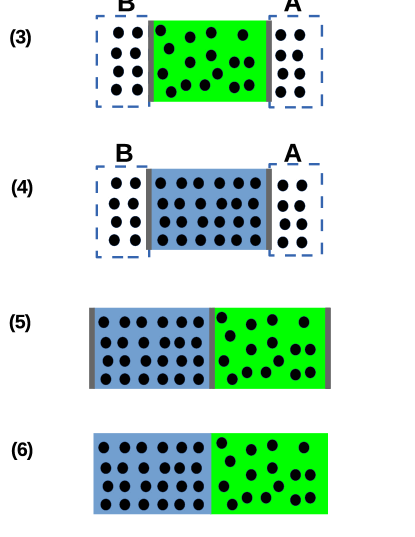
Figure 1: Sketch of the TI scheme to obtain $\gamma_{\rm cl}$. Particles in the blue and green simulation boxes represent the crystal and the liquid phase, respectively. For details see text.

The interfacial free energy $\gamma_{\rm cl}$ is the excess free energy required to form an interface between a crystal and a liquid at coexistence. Since it is an excess free energy, given by the difference between the free energies of a final and an initial state, it can be directly computed via TI. While the initial state is given by two independent systems, namely a bulk crystal and a bulk liquid at coexistence temperature and pressure, the final state is an inhomogeneous system where the liquid and the crystal phase are separated from each other by two interfaces. When constructing the reversible thermodynamic path between the initial and the final state, the bulk regions of the two phases should be perturbed as little as possible and no stress should be generated in the crystal when it gets in contact with the liquid.

A crucial step in our TI scheme is the introduction of an extremely short-ranged flat wall which is modelled by a repulsive Gaussian potential and placed at the boundaries of the simulation box in $z$ direction. The range of the particle interactions with this wall is chosen such that it is about $1000-10000$ times less than the typical size of the particles. Thus, the Gaussian wall only prevents the liquid and crystalline particles from crossing the boundaries of their simulation boxes but does not change the thermodynamic properties of the bulk system in any manner. Due to the extremely short-range nature of the wall, a very small time-step is needed to integrate the equations of motion in a molecular dynamics simulation. However, one can use a multiple time-step molecular dynamics algorithm to tackle this issue frenkel-smit02 and since only a few particles interact with the short-ranged wall, the additional computational overhead in implementing this algorithm is small (i.e. the simulations with Gaussian walls are less than a factor of two slower than corresponding simulations without these walls).

To ensure minimal perturbation of the crystal when the two phases are brought together, it is essential that the liquid is already ordered into crystalline layers near the interface, compatible with the actual crystal structure. In our TI scheme, this is achieved by introducing a structured solid wall, consisting of particles frozen into a configuration adopted in an actual simulation of the crystal phase. Interactions between the system and this structured wall were modelled by the same interaction potential as that between the system particles. Such a structured solid wall leads to formation of interfacial layers in the liquid which are more compatible with the actual crystal structure than if the structured wall consisted of particles fixed to an ideal crystal position as in Refs. davidchack-laird2000 ; davidchack-laird03 .

The starting points of our TI scheme are the simulations of a bulk crystal and a bulk liquid under coexistence conditions (see Sec. III.1). Both the liquid and the crystal are simulated in cubic boxes of identical dimensions ($L_{\rm x}\times L_{\rm y}\times L_{\rm z}$) but at their respective coexistence densities, assuming periodic boundary conditions in all spatial directions. The goal is to join simulation boxes with the liquid and the crystal phase along the $z$ direction and thereby create two independent crystal-liquid interfaces in equilibrium with the bulk phases (with the total dimension $L_{\rm x}\times L_{\rm y}\times 2L_{\rm z}$). Our TI scheme consists of the following sequence of steps to carry out this transformation (see Fig. 1):

Step 1: Insert an extremely short-ranged Gaussian flat wall at both ends of the liquid simulation box along the $z$ direction [sketch (1) in Fig. 1], while keeping the periodic boundary conditions intact. The wall should be strong enough to prevent the liquid particles from crossing the boundaries and be extremely short-ranged such that the interfacial free energy of the liquid in contact with this wall is negligible as compared to $\gamma_{\rm cl}$ (in our case, typically less than the statistical errors reported in previous works davidchack-laird03 ).

Step 2: Identical flat walls are inserted at the boundaries of the simulation box containing the crystal [(2) in Fig. 1] such that the distance of the closest crystalline layer from the flat wall is identical for both the left and right boundaries of the simulation cell.

Step 3: Two solid walls are constructed from the left and right parts of the crystal simulation cell near the two boundaries, containing 2-3 layers of crystalline particles. Then, these walls are gradually attached to the liquid simulation cell at the appropriate ends, with the flat walls still switched on, to prevent particles from crossing the boundaries. As shown in Fig. 1, the wall constructed from the left part of the crystal simulation cell is attached to the right end of the liquid simulation cell. Similarly, the wall made from the right side of the crystalline simulation cell is attached to the left side of the liquid phase. At the same time, the periodic boundary conditions of the liquid simulation cell in $z$ direction are gradually switched off. In this respect, this step is unlike the procedure adopted in previous TI schemes, where the boundary conditions are kept intact while switching on the “cleaving” walls.

Step 4: The same frozen-in parts of the crystal simulation cell are gradually introduced to the appropriate boundaries of the simulation box containing the actual crystalline phase, in presence of the flat walls, and simultaneously the periodic boundary conditions in the $z$ direction are turned off [cf. (4) in Fig. 1].

Step 5: The liquid and crystal systems are brought together and simultaneously the frozen-in crystalline walls are removed, in presence of the flat walls. This is accomplished by joining appropriate ends of the crystal and liquid simulation cells, where the flat walls are located. Doing this entails juxtaposing the solid wall in contact with one phase to be on top of the other phase. However, both phases interacted only with their respective solid walls. Since the periodic boundary conditions for the individual phases were already switched off, one needs only to switch on interactions between the two phases across the ends connected directly and also across the other end via gradually turning on the periodic boundary conditions [cf. (5) in Fig. 1]. This procedure is different from that followed by the “cleaving potential” or “cleaving walls” approach, where the liquid and crystal are first joined together and only in the next step, the “cleaving walls” are removed.

At the end of step 5, the system consists of crystal and liquid phases separated by two interfaces, whose position coincides with the position of the flat walls. Since, the crystal and liquid particles cannot cross the boundaries of their respective simulation cells, the position of the crystal-liquid interface is tied to the position of the flat walls. If we proceed in a reverse direction from the end of step 5, and then retrace each prior step, we will end up exactly from where the transformation started, i.e. the liquid and crystal phases at coexistence in separate simulation cells.

Step 6: Finally, in the last step, the extremely short-ranged Gaussian walls are gradually removed. When the the barrier imposed by the walls becomes weaker, the particles can cross the boundaries of their simulation cells. As a result the interfaces can move leading to hysteresis in the thermodynamic integration path. However, our scheme is successful in tackling the hysteresis arising from the mobility of the crystal-liquid interface, because the contribution of the last step to $\gamma_{\rm cl}$ is negligible (less than the combined statistical errors of steps 3, 4 and 5), on account of the extremely short-ranged flat walls. This ensures that any residual hysteresis in the last step is also reduced to a negligible amount, thus having no impact on the accuracy of the estimates. This is a more desirable way to circumvent the problem rather than the cumbersome approach of carrying out several forward and reverse TI runs of various durations and choosing the path with the least hysteresis davidchack-laird03 ; davidchack2010 .

In our TI calculations, we carry out the sequence of transformations outlined above by directly modifying the interaction potential of the flat walls and the frozen-in crystalline walls. This approach is similar to our earlier work on the determination of interfacial free energies of liquid or crystal phases in contact with flat or structured walls benjamin-horbach2012 ; benjamin-horbach2013 .

In all the steps of our TI scheme, the parameter $\lambda$ is coupled to the interaction potentials in a non-linear rather than a linear manner frenkel-smit02 . This is dictated by the need to obtain smooth thermodynamic integrands leading to an accurate numerical determination of the associated integrals. The particular choice for the $\lambda$-parameterizations adopted in the following are however, not unique, and other variants have been tried by us with identical results. In the following, we describe the specific manner in which the sequence of steps outlined above is carried out by coupling a parameter $\lambda$ to the interaction potential between the system and the walls.

Steps 1 and 2: Here, the interaction of a particle $i$ with an extremely short-ranged flat wall is modelled by a Gaussian potential,

$$u_{\text{fw}}(z_{iw})=a\exp\left[-\left(\frac{z_{iw}}{b}\right)^{2}\right]\,,$$ (4)

with $z_{iw}$ the distance of the particle from the wall in $z$-direction. The parameters $a$ and $b$ control the height of the potential barrier and the range of the potential, respectively. A suitable choice for $a$ is about 20-25 $k_{\rm B}T$ (with $k_{\rm B}$ the Boltzmann constant and $T$ the temperature of the system), which is sufficient to make the walls impenetrable for particles near the boundaries. The parameter $b$ is set to around 0.0001 $\sigma$–0.001 $\sigma$, i.e. a factor of 1000-10000 smaller than the typical size of the LJ particles. This choice of $b$ provides that the free energy contribution due to the Gaussian wall is much less than the statistical error bars in the most precise calculations of $\gamma_{\rm cl}$. The Gaussian flat walls are placed at the boundaries of the simulation cell at $z=0$ and $z=L_{\rm z}$.

A parameter $\lambda$ is coupled to the flat wall as follows,

$$\begin{split}u_{\text{fw}}(\lambda,z_{iw})=&\lambda^{2}u_{\text{fw}}(z_{iw})\end{split}$$ (5)

Thus, at $\lambda=0$, the Gaussian wall is zero, and as $\lambda$ increases the wall becomes more and more impenetrable and finally fully impenetrable at $\lambda=1$.

The $\lambda-$dependent Hamiltonian for steps 1 and 2 takes the form

$$\begin{split}H_{1,2}(\lambda)=\sum_{i=1}^{N}\frac{{{\bf p}_{i}^{2}}}{2m}+{U_{\text{pp}}^{\text{c(l)}}}+\lambda^{2}{U_{\text{fw}}^{\text{c(l)}}}\,,\end{split}$$ (6)

where, $H_{\rm 1}$ represents interaction of the flat wall with the liquid particles and $H_{\rm 2}$ those of the flat wall with the crystalline particles. In Eq. (6), ${\bf p}_{i}$ and $m$ represent the momentum and mass of particle $i$ with all particles have the same mass. The contribution from the particle-particle interactions to the potential energy is given by ${U_{\text{pp}}^{\text{c(l)}}}=\sum_{i=1}^{N^{\text{c(l)}}}\sum_{j=i+1}^{N^{\text{c(l)}}}u(r_{ij})$ with $r_{ij}$ the distance between two particles $i$ and $j$. The potential energy due to the interactions of particles with the flat wall is ${U_{\text{fw}}^{\text{c(l)}}}=\sum_{i=1}^{N^{\text{c(l)}}}u_{\text{fw}}(z_{\text{iw}})$, where the superscript $c(l)$ refers to particles in the crystal (liquid) phase and $N^{\text{c}}$ and $N^{\text{l}}$ are the total number of liquid and crystal particles, respectively. Dimensions of the simulation cells containing individual crystal and liquid phases are kept identical and as $\rho_{\rm l}<\rho_{\rm c}$, $N_{\rm c}<N_{\rm l}$.

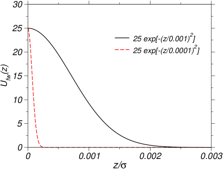
Figure 2: Gaussian flat wall potential for $b=10^{-3}\,\sigma$ (black solid line) and $b=10^{-4}$ (red dashed line); in both cases, the barrier height is set to $a=25\,\epsilon$, as used for $T=1.0$. For $T=0.617$ and $T=1.5$, the latter parameter was set to $a=15\,\epsilon$ and $a=35\,\epsilon$, respectively.

The free energy differences, $\Delta F_{1}$ and $\Delta F_{2}$, in steps 1 and 2 are obtained via the following integration over the parameter $\lambda$,

$$\Delta F_{1,2}=\int_{0}^{1}\left\langle\frac{\partial H_{1,2}}{\partial\lambda}\right\rangle d\lambda=\int_{0}^{1}\left\langle 2\lambda{U_{\text{fw}}^{\text{c(l)}}}\right\rangle d\lambda\,.$$

Since the crystal can translate along the $z$ direction, it is not guaranteed that the crystal is symmetrically positioned with respect to the left and right boundaries in $z$ direction. This creates a problem in the subsequent steps. Since the solid walls inserted in steps 3 and 4 are made of frozen-in crystalline layers near the two ends of the crystal simulation cell, such asymmetry in the position of the crystal will lead to two dissimilar solid walls being made to come in contact with the liquid and crystal phases on either side. This would lead to an ordering in the liquid phase which is not compatible with the actual crystal structure. Similarly, two walls with their outermost layers at different distances from the two sides of the crystal phase might lead to stresses in the crystal.

To avoid this, the two innermost layers of the crystalline phase were frozen such that the crystalline phase was symmetric with respect to the two boundaries. This ensured that the solid walls generated from such a symmetric crystal were similar and their outermost layers were at the same average distance from the two boundaries. This is similar to what was done in the “cleaving wall” approach davidchack-laird03 . Freezing the innermost layers did not have any additional side effects on the crystal-liquid interface, as was verified by carrying out simulations with both larger and shorter $L_{\rm z}$.

Steps 3 and 4: The $\lambda$-dependent Hamiltonian for steps 3 and 4 is chosen as follows,

$$\begin{split}H_{3,4}(\lambda)=\sum_{\text{i=1}}^{N}\frac{{\bf p}_{i}^{2}}{2m}+{{U}_{\text{pp}}^{\text{c(l)}}}+(1-\lambda)^{3}{{U^{\ast}}_{\text{pp}}^{\text{c(l)}}}\\ +\lambda^{10}{U_{\text{pw}}^{\text{c(l)}}}+{U_{\text{fw}}^{\text{c(l)}}}\end{split}$$ (7)

where $H_{3}$ includes the interactions of the structured wall with the liquid particles and $H_{4}$ those of the structured wall with the crystalline particles. ${{U^{\ast}}_{\text{pp}}^{\text{c(l)}}}$ represents interactions between particles through the periodic boundaries along the $z$ direction, while ${U_{\text{pp}}^{\text{c(l)}}}$ corresponds to direct interactions. ${U_{\text{pw}}^{\text{c(l)}}}=\sum_{i=1}^{N^{\text{c(l)}}}\sum_{j=1}^{N^{\text{w}}}u_{\text{pw}}(r_{{ij}})$, where $N^{\text{w}}$ is the total number of particles comprising the frozen walls and interactions between the system and the structured wall particles is denoted by $u_{\text{pw}}$. For $u_{\text{pw}}$ the potential given by Eqs. (2) and (3) was used, replacing the parameter $\epsilon$ by $\epsilon_{\rm pw}$. In step 3, $\epsilon_{\rm pw}$ varied between $0.54\,\epsilon$ and $1.0\,\epsilon$ (depending on the considered temperatures), while in step 4, $\epsilon_{\rm pw}=1.0\,\epsilon$ was set. These choices of $\epsilon_{\rm pw}$ ensured that the bulk densities of the liquid and crystal phases remained unperturbed throughout the integration path.

The free energy differences for steps 3 and 4 are obtained as

$$\Delta F_{3,4} = \int_{0}^{1}\left\langle\frac{\partial H_{3,4}}{\partial\lambda}\right\rangle d\lambda$$ (8)

$$= -\int_{0}^{1}\left\langle 3(1-\lambda)^{2}{{U^{\ast}}_{\text{pp}}^{\text{c(l)}}}\right\rangle d\lambda$$

$$+\int_{0}^{1}\left\langle 10\lambda^{9}{U_{\text{pw}}^{\text{c(l)}}}\right\rangle d\lambda\;.$$

Since we directly modify the interaction potential between the structured solid wall and the system particles and the system particles cannot cross the boundaries of their simulation boxes due to the repulsive Gaussian flat walls, there is no need of adopting any “corrugated cleaving plane” as was introduced in Refs. davidchack-laird03 ; davidchack2010 .

Step 5: In this step, the Hamiltonian is given by

$$\begin{split}H_{5}(\lambda)=\sum_{\text{i=1}}^{N_{p}}\frac{{\bf p}_{\text{i}}^{2}}{2m_{i}}+{{{U}_{\text{pp}}^{\text{c(l)}}}}+\lambda^{5}{U_{\text{pp}}^{\text{c+l}}}\\ +(1-\lambda)^{5}{U_{\text{pw}}^{\text{c(l)}}}+{U_{\text{fw}}^{\text{c(l)}}}\end{split}$$ (9)

where ${U_{\text{pp}}^{c+l}}=\sum_{i=1}^{N^{\text{l}}}\sum_{j=1}^{N^{\text{c}}}u(r_{{ij}})$ corresponds to interaction between a liquid particle (with index $i$) and a crystalline particle (with index $j$).

The free-energy difference for step 5 is

$$\Delta F_{5} = \int_{0}^{1}\left[\left\langle\frac{\partial H_{5}}{\partial\lambda}\right\rangle\right]d\lambda$$ (10)

$$= 5\int_{0}^{1}\langle\lambda^{4}{U_{\text{pp}}^{\text{c+l}}}\rangle\,d\lambda$$

$$-5\int_{0}^{1}\langle(1-\lambda)^{4}{U_{\text{pw}}^{\text{c(l)}}}\rangle\,d\lambda\,.$$

The interaction strength between the structured wall and the liquid and crystal particles was kept at the same value of $\epsilon_{\rm pw}$ as in steps three and four, respectively.

Step 6: In the last step, the Gaussian flat walls are gradually switched off. In this case, the following $\lambda$ parametrization is used for $u_{\rm fw}$,

$$\begin{split}u_{\text{fw}}(\lambda,z_{iw})=&(1-\lambda)^{2}u_{\text{fw}}(z_{\text{iw}})\,,\end{split}$$ (11)

and the $\lambda$-dependent Hamiltonian for this step takes the form,

$$\begin{split}H_{6}(\lambda)=\sum_{i=1}^{N_{\rm p}}\frac{{{\bf p}_{i}^{2}}}{2m}+{{{U}_{\text{pp}}^{\text{c(l)}}}}+{U_{\text{pp}}^{\text{c+l}}}+{(1-\lambda)^{2}}{U_{\text{fw}}^{\text{c(l)}}}\end{split}$$ (12)

and thus the free energy difference for step 6 is

$$\Delta F_{6}=\int_{0}^{1}\left\langle\frac{\partial H_{6}}{\partial\lambda}\right\rangle d\lambda=\int_{0}^{1}\left\langle 2(\lambda-1){U_{\text{fw}}^{\text{c(l)}}}\right\rangle d\lambda$$ (13)

The interfacial free energy is finally obtained by summing over the equilibrium free energy differences for the six sequential transformations and the division by the total interfacial area $A$,

$$\gamma_{\rm cl}=\frac{{\Delta F}_{1}+{\Delta F}_{2}+{\Delta F}_{3}+{\Delta F}_{4}+{\Delta F}_{5}+{\Delta F}_{6}}{A}\,,$$ (14)

with $A=2L_{\rm x}L_{\rm y}$ (note that the factor 2 takes into account that due to the periodic boundary conditions there are two independent planar crystal-liquid interfaces, cf. Fig. 1).

The TI scheme proposed in this work contains six steps as opposed to the four steps involved in the “cleaving potential” or “cleaving walls” scheme. However, contributions from steps one, two and six are negligible on account of the very short-ranged flat walls. As our results in Sec. IV indicate, these contributions are less than the total statistical errors from steps three, four and five. Therefore, one could start with independent liquid and crystal phases in contact with Gaussian flat walls and end with two crystal-liquid interfaces in equilibrium with the bulk phase and in presence of such short-ranged walls and be still able to obtain reliable estimates for $\gamma_{\rm cl}$. We also want to point out that such short-ranged Gaussian walls do not suppress capillary wave fluctuations morris2002 ; rozas2011 ; schmitz2014 but only prevent the movement of the two crystal-liquid interfaces.

III.1 Simulations

Molecular dynamics (MD) computer simulations are performed at constant particle number $N$, constant volume $V$, and constant temperature $T$. To keep the temperature constant, the velocities of the particles were drawn from a Maxwell-Boltzmann distribution at the desired temperature every $200$ time steps. To integrate the equations of motion, the velocity form of the Verlet algorithm allen-tildesley87 is used. We use a multiple-time step scheme frenkel-smit02 to take into account the short-range forces due to the Gaussian wall. For this purpose, a smaller time step of $\Delta t_{\rm small}=0.00025\,\tau$ was used in conjunction with a larger time-step of $\Delta t_{\rm large}=0.004\,\tau$, where $\tau=\sqrt{(m\sigma^{2}/\epsilon)}$.

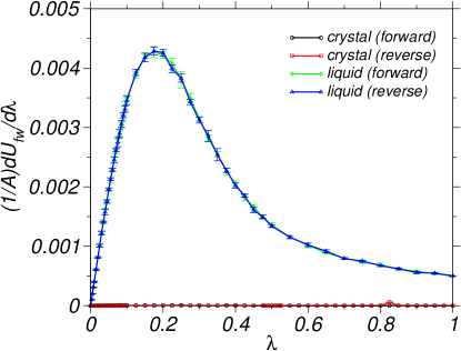
Figure 3: Thermodynamic integrand for steps 1 and 2 for the liquid and crystal phases, respectively, at $T=1.0$ and the (100) orientation of the crystal. Error bars in this figure and subsequent ones represent one standard deviation.

The density $\rho=N/V$ of the crystal and liquid at coexistence, corresponding to the modified LJ potential considered in this work, were taken from Ref. davidchack-laird03 . We consider three different coexistence temperatures at $T=0.617$, 1.00, and 1.50. The coexistence densities of the crystal and liquid, $\rho_{\rm l}$ and $\rho_{\rm c}$, respectively, at these temperatures are as follows: $\rho_{l}=0.8282$ and $\rho_{c}=0.945$ at $T=0.617$ and a coexistence pressure $P=-0.02$, $\rho_{l}=0.923$ and $\rho_{c}=1.0044$ at $T=1.00$ and a coexistence pressure $P=4.95$ and $\rho_{\rm l}=1.003$ and $\rho_{\rm c}=1.074$ at $T=1.50$ and a coexistence pressure $P=12.95$. All the pressure values are in reduced units, $\sigma^{3}/k_{B}T$. We have verified the coexistence densities by carrying out simulations of crystal-liquid interfaces and checking the densities of the crystal and liquid in the bulk. Independent simulations of bulk crystal and liquid were also carried out at these densities and it was confirmed that the coexistence pressures in both the bulk liquid and bulk crystal were identical within the statistical error.

The parameters $a$ and $b$ appearing in the Gaussian flat wall potential have to be chosen carefully such that the wall is extremely short-ranged. At the same time, when it is fully applied no particles should cross the barrier imposed by this short-ranged wall. Taking these two factors into account, $a$ was taken to be $15.0\epsilon$, $25.0\epsilon$ and $35.0\epsilon$ at the co-existence temperatures $T=0.617$, $1.0$ and $1.5$, respectively. At each temperature, $b$ was chosen to take the value $0.001\sigma$, which made the wall sufficiently short-ranged. Nevertheless, we also tried another wall with an even shorter range i.e. $b=0.0001\sigma$ but obtained identical results within the statistical error.

System sizes for the various coexistence temperatures and orientations of the crystal were the same as in Ref. davidchack-laird03 . Only at $T=1.0$ and for the (100) orientation of the crystal-liquid interface, simulations were carried out for various system sizes, corresponding to several combinations of lateral ($L_{\rm x}$, $L_{\rm y}$) and longitudinal ($2L_{\rm z}$) system sizes. The dimensions of the simulation boxes are specified in Table I. For the considered system sizes, the total number of particles varied from $N=6000$ to about $N=32000$.

To generate initial configurations, the liquid and crystal phases were equilibrated at the coexistence temperatures and their respective coexistence densities. Dimensions of the liquid and crystal simulation cells were identical and since $\rho_{\rm l}<\rho_{\rm c}$, correspondingly less number of particles were contained in the liquid simulation cell. After each phase was equilibrated for around $200000$ time steps (here and later on, in multiples of the larger time-step $\Delta t_{\rm large}$), the TI simulations were started.

For the TI calculations, independent runs were carried out at various values of $\lambda$ between $0$ and $1$. For the various TI steps, the total number of intervals between $\lambda=0$ and $\lambda=1$ varied from $45$ to $50$, which was sufficient to produce smooth thermodynamic integrands. At each value of $\lambda$, i.e. $\lambda_{i}$, the system was equilibrated at $\lambda=0$ for $10000$ time steps and then $\lambda$ was continuously increased until $\lambda_{i}$ was reached. The number of time-steps to carry out this switch varied from $90000$ to $150000$ time-steps for the various system sizes and various orientations. After the final value $\lambda_{i}$ was reached, the system was further equilibrated for $500000-750000$ time-steps. Then the production runs were carried out over a period ranging from $250000$ to $500000$ time-steps. Statistical errors were determined by dividing the production runs into $5$ blocks and then obtaining the standard deviation between these $5$ samples.

To calculate the free energy difference from the obtained thermodynamic integrands for steps 3, 4 and 5, we did a cubic spline interpolation of the bare data with 100 intervals between $\lambda=0$ and $\lambda=1$ and then used the Simpson rule to numerically calculate the integral. For steps 1, 2 and 6, the numerical integration was carried out over the bare data using the trapezoidal rule.

We have carried out simulations in both the forward and reverse directions to detect any residual hysteresis in the TI path. The initial state for the reverse TI simulations were taken from the final state of the forward TI path. The final values for $\gamma_{\rm cl}$ reported in the next section correspond to a mean of the free energy differences obtained from the forward and reverse TI simulations.

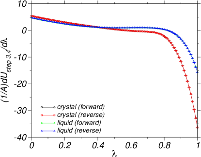
Figure 4: Thermodynamic integrand corresponding to steps 3 and 4, for the liquid and (100) orientation of the crystal, respectively, at the temperature $T=1.0$.

IV Results

In Figs. 3, 4, 5, and 6, the thermodynamic integrands corresponding to the six steps are plotted for the (100) orientation of the crystal-liquid interface at $T=1.0$. Here, the system size of the final state with two interfaces is $14.263\sigma\times 14.263\sigma\times 31.695\sigma$. In all figures we show the thermodynamic integrands for both the forward (increasing $\lambda$ from $0$ to $1$) and reverse (decreasing $\lambda$ from $1$ to $0$) processes. The final values of the interfacial free energy for the various cases are reported in Table 1 and the errors include both the statistical error and the residual hysteresis between the forward and reverse paths.

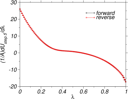
Figure 5: Thermodynamic integrand for step 5 at $T=1.0$, bringing the (100) orientation of the crystal in contact with the liquid.

In Fig. 3, we show the thermodynamic integrands for inserting the Gaussian flat wall (and removing for the reverse process) into the crystal and liquid phases, respectively. Good overlap of the forward and reverse thermodynamic integrands indicates, as expected, the lack of hysteresis in our TI scheme. As can be clearly seen in the figure, the area under the thermodynamic integrand corresponding to the crystal in contact with the flat wall is negligible as compared to the same situation for the liquid. On account of the extremely short range of the flat walls, very few particles actually interact with them leading to a negligible contribution to the free energy difference. Since the crystal is placed symmetrically with respect to the two ends of the simulation cell, the flat walls are located in the middle of two crystalline layers. Therefore, their position coincides with a minimum of the crystal density leading to a negligible value for the free energy difference as compared to the liquid.

The interfacial free energy of the liquid in contact with the flat wall is $0.0018k_{B}T$ at $T=1.0$ when $b=0.001\sigma$, which is of the order of $<0.35\%$ of the final value of $\gamma_{\rm cl}$. In case of the crystal, the contribution of this flat wall varies from $\sim 10^{-7}\,k_{\rm B}T$ for the (111) orientation to $10^{-6}k_{\rm B}T$ for the (100) orientation and $10^{-5}k_{\rm B}T$ for the (110) orientation. For this choice of $b$, the combined contribution of step 1 and step 2 was lower than the statistical errors in the most precise estimates of $\gamma_{\rm cl}$.

In the next two steps, liquid and crystalline phases were separately brought into contact with structured solid walls in presence of the Gaussian flat wall and simultaneously the periodic boundary conditions were switched off. Thermodynamic integrands corresponding to steps 3 and 4 are shown in Fig. 4. In step 3, the interaction strength $\epsilon_{\rm pw}=1.0\,\epsilon$ was chosen at $T=0.617$, while at the other temperatures $\epsilon_{\rm pw}=0.54\,\epsilon$. For the interaction of the crystal with the structured wall, at all temperatures $\epsilon_{\rm pw}$ was set to $1.0\,\epsilon$. As the $\lambda$ parameter is gradually increased, the liquid begins to form ordered layers near the interface due to interactions with the solid wall. This process was the source of some hysteresis in the “cleaving walls” davidchack-laird03 and “cleaving potentials” broughton-gilmer86 scheme, though it could be avoided by equilibrating the samples for longer times.

The smooth variation of the thermodynamic integrands corresponding to steps 3 and 4 (see Fig. 4) along with small error bars throughout the integration path indicates that our system was well equilibrated and not trapped in some metastable state. The excellent overlap between the thermodynamic integrands for the forward and reverse processes also confirms the reversibility of our TI scheme.

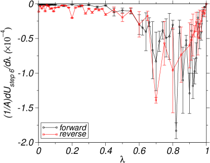
Figure 6: Thermodynamic integrand for the last step, corresponding to switching off the flat wall.

In the next step, the liquid and crystal were joined together, while the interactions of the liquid and crystal phases with the frozen walls were switched off. As Fig. 5 shows, the integrands are smooth leading to an accurate numerical determination of the integral. The forward and reverse thermodynamic integrands are also in very good agreement. In the “cleaving potential” and “cleaving walls” approach, the liquid and crystal phases were first brought together and then the walls were removed. However, in our scheme these steps are combined into a single step. Nevertheless, we carried out TI simulations where our single step scheme was divided into two steps: first bringing the two phases together and in the next step removing the structured walls, while varying the parameter $\lambda$ in exactly the same manner as specified in Eq. 9. However, both approaches led to identical results.

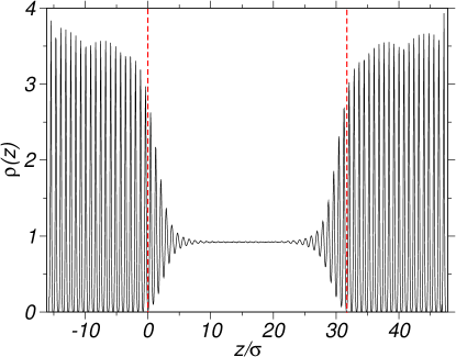
Figure 7: Density profile of the (100) orientation of the crystal in contact with the liquid and separated by a short-ranged flat wall. The temperature is $T=1.0$. Red vertical lines correspond to the positions of the flat walls. The system size is $14.263\,\sigma\times 14.263\,\sigma\times 31.695\sigma$.

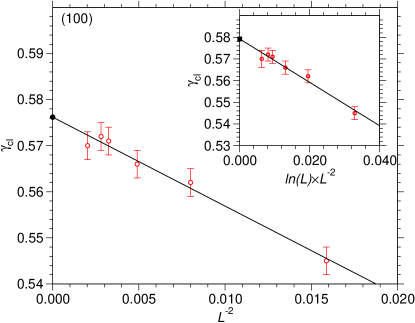
Figure 8: $\gamma_{\rm cl}$ vs. $1/L^{2}$, where $L=L_{\rm x}=L_{\rm y}$, corresponding to the (100) orientation of the crystal-liquid interface with the longitudinal dimension $L_{\rm z}=31.695\,\sigma$. For the same parameters, the inset shows $\gamma_{\rm cl}$ vs. $\ln(L)/L^{2}$. Solid symbols correspond to the $\gamma_{\rm cl}$ values in the thermodynamic limit.

The final step involves removing the flat walls. However, this process is no longer reversible after the barrier posed by the flat wall becomes weaker and the crystal-liquid interfaces can move. This is reflected in the hysteresis between the forward and reverse thermodynamic integrands, as shown in Fig. 6. However, the contribution of this step is negligible owing to the short-range nature of the flat walls. Figure 6 clearly shows that the area under both the forward and reverse thermodynamic integrands is much smaller, in magnitude, as compared to step 1. As a result, one does not need to follow the “cleaving walls” approach of carrying out several forward and reverse simulation runs to estimate the path with the least hysteresis. In fact, for the (100) orientations of the crystal-liquid interface both forward and reverse simulations predict a magnitude less than $10^{-4}\,k_{\rm B}T$ for this step. This contribution will be negative since the flat wall is purely repulsive and we are removing it (see Eq. 13 and Fig. 6). Similarly negligible contributions are obtained for the other two orientations as well.

To understand why ${{\Delta F}_{6}}/A$ would be negligible, in Fig. 7 we plot the density profile corresponding to the (100) orientation of the crystal-liquid interfaces in equilibrium with their bulk phases. If the minima of the density profile coincides with the flat wall position, one will obtain a negligible contribution as in step 2. On the other hand if a maxima coincides, the result would be larger, though due to a finite barrier imposed by the repulsive Gaussian walls, the probability of a maxima in the density profile coinciding with the wall position is small.

In the first step, the free energy difference per unit area was around $0.0018k_{B}T$ (at $T=1.0$). Since, we observe that the maxima in the density profile is about 3 times that of the bulk liquid, it is clear that the maximum possible magnitude for ${{\Delta F}_{6}}/A$ would be 3 times the contribution of ${{\Delta F}_{1}}/A$ and therefore would still be significantly smaller than $\gamma_{\rm cl}$. Since the interfaces can move by simultaneous melting and freezing, the average density of the inhomogeneous system near the positions of the flat wall would be much smaller. Therefore, the actual free energy difference in the last step would be much less than this maximum possible value.

Temperature	Orientation	System Size	$\gamma_{\rm cl}$(TI)	Cleaving Wall	Non-Eq. Work
$1.000$	$100$	$7.924\times 7.924\times 31.695$	$0.545\pm 0.003$	—	—
$1.000$	$100$	$11.093\times 11.093\times 31.695$	$0.562\pm 0.004$	—	—
$1.000$	$100$	$14.263\times 14.263\times 31.695$	$0.566\pm 0.003$	$0.562\pm 0.006$	—
$1.000$	$100$	$19.017\times 19.017\times 20.602$	$0.572\pm 0.003$	—	—
$1.000$	$100$	$17.432\times 17.432\times 31.695$	$0.571\pm 0.003$	—	—
$1.000$	$100$	$19.017\times 19.017\times 31.695$	$0.572\pm 0.003$	—	—
$1.000$	$100$	$19.017\times 19.017\times 41.204$	$0.569\pm 0.004$	—	—
$1.000$	$100$	$22.187\times 22.187\times 31.695$	$0.570\pm 0.003$	—	—
$1.000$	$100$	$\infty$	$0.576^{\rm a},0.579^{\rm b}$	—	—
$1.000$	$110$	$14.263\times 13.447\times 26.894$	$0.545\pm 0.003$	$0.543\pm 0.006$	—
$1.000$	$111$	$11.646\times 12.327\times 32.939$	$0.515\pm 0.006$	$0.508\pm 0.008$	—
$0.617$	$100$	$14.559\times 14.559\times 32.352$	$0.372\pm 0.005$	$0.371\pm 0.003$	$0.371\pm 0.004$
$0.617$	$110$	$14.559\times 13.726\times 27.452$	$0.357\pm 0.003$	$0.360\pm 0.003$	$0.361\pm 0.003$
$0.617$	$111$	$11.887\times 12.582\times 33.622$	$0.344\pm 0.006$	$0.347\pm 0.003$	$0.354\pm 0.003$
$1.500$	$100$	$13.951\times 13.951\times 31.001$	$0.866\pm 0.005$	$0.84\pm 0.02$	—
$1.500$	$110$	$13.951\times 13.153\times 26.306$	$0.785\pm 0.006$	$0.82\pm 0.02$	—
$1.500$	$111$	$11.391\times 12.057\times 32.218$	$0.774\pm 0.007$	$0.75\pm 0.03$	—

Table 1: Interfacial free energy $\gamma_{\rm cl}$ for different system sizes corresponding to various orientations of the crystal-liquid interface, three different co-existence temperatures and different system sizes. For comparison, data from the cleaving wall davidchack-laird03 and non-equilibrium work apporaches musong2006 are also shown. Dimensions ($L_{\rm x}\times L_{\rm y}\times L_{\rm z}$) are in units of $\sigma^{3}$. At $T=1.0$ and for the (100) orientation of the crystal-liquid interface, the interfacial free energy in the thermodynamic limit is extrapolated from the values of $\gamma_{\rm cl}$ at the various system sizes using the (a) $L^{-2}$ and (b) $\ln(L)L^{-2}$ scalings (see text).

In principle, one can make the Gaussian flat walls as short-ranged as possible to reduce their contribution even further. However, reducing the range involves a concomitant increase in computational cost due to the need for a very short time-step in the multiple-time step scheme. A slightly more efficient way to reduce the hysteresis, would be to use a Gaussian flat wall with a range long enough that one can use the regular single time-step velocity-verlet algorithm and at the same time sufficiently short-ranged, so as not to affect the bulk density of the phases. One can carry out steps 1-5 of the TI scheme with this flat wall, with no computational overhead involved in a multiple-time step scheme. In the next step, one can first transform this flat wall to an extremely short-ranged wall. The parametrization for this step, which we call step 6a, will be

$$\begin{split}u_{\text{fw}}(\lambda,z)=&a\exp(-[z/b(\lambda)]^{2})\,,\end{split}$$ (15)

where $b(\lambda)=(1-\lambda)b^{\prime}$ with $b^{\prime}=0.001\sigma$ and $\lambda$ varying from $0$ to $0.9$. This step will be subject to minimal hysteresis as the flat walls are still present to prevent the particles from crossing boundaries of their simulation cells. The average position of the crystal-liquid interface would oscillate around the position of the flat walls. In the next step (step 6b) one can remove the flat walls with the same parametrization as in Eq. (8).

We have carried out simulations by breaking step six into the two steps as specified here and obtained results in perfect agreement with the earlier method, since the flat wall chosen for our simulations was already extremely short-ranged. However, this latter approach of using an extremely short-ranged wall only in the final step, will be useful for long-ranged potentials, where the computational overhead of using a multiple time-step scheme for all the six steps might become significant.

The flat Gaussian walls can, in principle, be adapted to any continuous potential. Only the prefactor $a$, which sets the height of the barrier needs to be modified to adapt the barrier height at different temperatures. The value for the parameter $b$ would be suitable for most potentials, and in cases where $\gamma_{\rm cl}$ has a small magnitude, the approach of breaking down step six into two steps would be also useful.

In Table I, we report the final values of $\gamma_{\rm cl}$ for different orientations, system sizes and temperatures. We also report data from the cleaving wall method davidchack-laird03 and a non-equilibrium work approach musong2006 . Clearly, our results are in good agreement with both the methods.

While $\gamma_{\rm cl}$ can be computed by various molecular simulation techniques, often there is disagreement between them which is greater than the statistical errors. For example, values for the hard-sphere interfacial free energy predicted by the “cleaving wall” approach is more than $10\%$ less than the one computed using the capillary fluctuation method or the tethered Monte Carlo approach. In a recent work, Schmitz et al. schmitz2014 suggested systematic errors arising out of finite size effects to be a possible source of disagreement between the various methods. They identified the mechanism of finite size corrections and proposed a theoretical tool to obtain reliable estimates for interfacial tensions in the thermodynamic limit.

In a three-dimensional system, if a planar interface is described by a lateral dimension $L=L_{\rm x}=L_{\rm y}$ and a longitudinal dimension $L_{\rm z}$, the leading finite size corrections to the interfacial free energy in the thermodynamic limit, $\gamma_{\rm\infty}$, are described by the following formula schmitz2014 ; binder82 :

$$\gamma_{\rm L,L_{\rm z}}=\gamma_{\rm\infty}-a\frac{\ln L_{\rm z}}{L^{2}}+b\frac{\ln L}{L^{2}}+\frac{c}{L^{2}}\,$$ (16)

where $a$, $b$ and $c$ are constants. To study the finite size corrections in our system, we carried out simulations for various lateral dimensions of the crystal-liquid interface for the (100) orientation of the crystal-liquid interface at $T=1.0$.

In Eq. (16), the second term is associated with the translational entropy of the interface due to movement of the crystal-liquid interface. Since, the flat walls constrain the movement of the crystal-liquid interface this term is negligible in our case and can be neglected. In Fig. 8, we plot the interfacial free energy for the (100) interface as a function of $1/L^{\rm 2}$ and $\ln(L)/L^{\rm 2}$ (in the inset), at the longitudinal system size, $L_{\rm z}=31.695\sigma$. A linear extrapolation of the data provides $\gamma_{\rm cl}$ in the thermodynamic limit and for the $1/L^{\rm 2}$ scaling we obtain a value of $0.576$, while for the $\ln(L)/L^{\rm 2}$ scaling a value of $0.579$ is obtained. Compared to the estimated value of $\gamma_{\rm cl}$ at the lateral dimension studied by Davidchack and Laird davidchack-laird03 , viz. $14.263\sigma\times 14.263\sigma$, these values are larger by about $2\%$.

V Conclusion

We have obtained the crystal-liquid interfacial free energy for the Lennard-Jones potential via a novel thermodynamic integration scheme. A crucial lacunae of previous thermodynamic integration schemes pertaining to the movement of the crystal liquid interface has been overcome by the help of extremely short-ranged Gaussian walls. Another feature of our scheme is the use of frozen-in crystalline layers to induce ordering in the liquid and thereby merge the crystal and liquid in a smooth manner. Our results are in good agreement with previous methods based on the cleaving method davidchack-laird03 as well as a non-equilibrium work approach musong2006 . Using the finite-size scaling for the (100) orientation, we have extrapolated the finite-size data to obtain $\gamma_{\rm cl}$ in the thermodynamic limit.

Aside from our TI scheme with flat walls, other schemes such as the ones proposed by Schilling and Schmid schilling-schmid2009 or by Grochola grochola2004 could, in principle, be used to overcome the problem related to movement of the crystal-liquid interface. However, such schemes involve modifying the interaction potential of the entire system, yielding large free energy differences and as a result the statistical errors are of the same order of magnitude as $\gamma_{\rm cl}$ itself. Therefore, such schemes have to be substantially modified to compute $\gamma_{\rm cl}$.

In a recent work, $\gamma_{\rm cl}$ for the modified LJ potential has been obtained using density functional theory wangdft2013 , with values in reasonable agreement with our data. The precise estimates for the interfacial free energy could be used to further refine and validate density functional theory approaches.

The thermodynamic integration scheme developed in this work can be used to obtain the interfacial free energies of systems described by more complex potentials or also of hard sphere systems, with only minor modification of the coupling of the parameter $\lambda$ to the interaction potentials. Work in this direction is the subject of forthcoming studies.

- (1) D. Turnbull and R. E. Cech, J. Appl. Phys. 21, 804 (1950).
- (2) D. Turnbull, J. Appl. Phys. 21, 1022 (1950).
- (3) D. Turnbull, J. Chem. Phys. 20, 411 (1952).
- (4) D. Woodruff, The Solid-Liquid Interface, 1st ed. (Cambridge University Press, London, 1973).
- (5) W. A. Tiller, The Science of Crystallization: Microscopic Interfacial Phenomena (Cambridge University Press, New York, 1991).
- (6) J. Q. Broughton and G. H. Gilmer, J. Chem. Phys. 84, 5759 (1986).
- (7) K. Kelton, Solid State Physics, 1st ed., (Academic Press, Dordrecht, 1991).
- (8) J. Bokeloh, R. E. Rozas, J. Horbach, and G. Wilde, Phys. Rev. Lett. 107, 145701 (2011).
- (9) J. Bokeloh, G. Wilde, R. E. Rozas, R. Benjamin, and J. Horbach, Eur. Phys. J. – ST 223, 511 (2014).
- (10) T. Palberg, submitted to J. Phys.: Condens. Matter (preprint).
- (11) H. E. A. Huitema, M. J. Vlot and J. P. van der Eerden, J. Chem. Phys. 111, 4714 (1999).
- (12) H. L. Tepper and W. J. Briels, J. Chem. Phys. 116, 5186 (2002).
- (13) B. B. Laird and A. D. J. Hamet, Chem. Rev. 92, 1819 (1992).
- (14) R. L. Davidchack and B. B. Laird, Phys. Rev. E 54, R5905 (1996).
- (15) R. L. Davidchack and B. B. Laird, J. Chem. Phys. 108, 9452 (1998).
- (16) J. J. Hoyt, M. Asta, and A. Karma, Phys. Rev. Lett. 86, 5530 (2001).
- (17) J. R. Morris, J. Chem. Phys. 66, 144104 (2002).
- (18) J. R. Morris and X. Song, J. Chem. Phys. 119, 3920 (2003).
- (19) R. L. Davidchack, J. R. Morris, and B. B. Laird, J. Chem. Phys. 125, 094710 (2006).
- (20) M. Amini and B. B. Laird, Phys. Rev. B 78, 144112 (2008).
- (21) T. Zykova-Timan, R. E. Rozas, J. Horbach, and K. Binder, J. Phys.: Condens. Matter 21, 464102 (2009).
- (22) T. Zykova-Timan, J. Horbach, and K. Binder, J. Chem. Phys. 133, 014705 (2010).
- (23) R. E. Rozas and J. Horbach, EPL 93, 26006 (2011).
- (24) A. Härtel, M. Oettel, R. E. Rozas, S. U. Egelhaaf, J. Horbach, and H. Löwen, Phys. Rev. Lett. 108, 226101 (2012).
- (25) V. Heinonen, A. Mijailovic, C. Achim, T. Ala-Nissila, R. E. Rozas, J. Horbach, and H. Löwen, J. Chem. Phys. 138, 044705 (2013).
- (26) L. A. Fernandez, V. Martin-Mayor, B. Seoane, and P. Verrocchio, Phys. Rev Lett. 108, 165701 (2012).
- (27) S. Angioletti-Uberti, M. Ceriotti, P. D. Lee, and M. W. Finnis, Phys. Rev. B 81, 125416 (2010).
- (28) S. Angioletti-Uberti, J. Phys.: Condens. Matter 23, 435008 (2011).
- (29) R. L. Davidchack and B. B. Laird, Phys. Rev. Lett. 85, 4751 (2000).
- (30) R. L. Davidchack and B. B. Laird, J. Chem. Phys. 118, 7651 (2003).
- (31) R. L. Davidchack and B. B. Laird, Phys. Rev. Lett. 94, 086102 (2005).
- (32) B. B. Laird and R. L. Davidchack, J. Phys. Chem. B 109, 17802 (2005).
- (33) R. L. Davidchack, J. Chem. Phys. 133, 234701 (2010).
- (34) F. Turci, T. Schilling, M. H. Yamani, and M. Oettel, Eur. Phys. J. – ST 223, 421 (2014).
- (35) F. Turci and T. Schilling, preprint arXiv:1405.5112.
- (36) D. Frenkel and B. Smit, Understanding Molecular Simulation (Academic, San Diego, 2002).
- (37) T. P. Straatsma, M. Zacharias, and J. A. MacCammon, Computer Simulations of Biomolecular Systems (Escom, Keiden, 1993).
- (38) A. W. Adamson and A. P. Gast, Physical chemistry of surfaces (Wiley-Interscience, New York, 1997).
- (39) V. G. Baidakov, S. P. Protsenko, and A. O. Tipeev, J. Chem. Phys. 139, 224703 (2013).
- (40) J. Wang et al., J. Chem. Phys. 139, 114705 (2013).
- (41) P. A. Apte, J. Chem. Phys. 132, 084101 (2010).
- (42) Y. Mu and X. Song, Phys. Rev. E 74, 031611 (2006).
- (43) C. Jarzynski, Phys. Rev. Lett. 78, 2690 (1997).
- (44) C. Jarzynski, Phys. Rev. E 73, 046105 (2006).
- (45) K. Binder, Phys. Rev. A 25, 1699 (1982).
- (46) F. Schmitz, P. Virnau, and K. Binder, Phys. Rev. Lett. 112, 125701 (2014).
- (47) R. Benjamin and J. Horbach, J. Chem. Phys. 137, 044707 (2012); J. Chem. Phys. 139, 039901 (2013).
- (48) R. Benjamin and J. Horbach, J. Chem. Phys. 139, 084705 (2013).
- (49) M. P. Allen and D. J. Tildesley, Computer Simulations of Liquids (Clarendon, Oxford, 1987).
- (50) T. Schilling and F. Schmid, J. Chem. Phys. 131, 231102 (2009).
- (51) G. Grochola, J. Chem. Phys. 120, 2122 (2004).
- (52) X. Wang, J. Mi, and C. Zhong, J. Chem. Phys. 138, 164704 (2013).