A lower bound for the number of negative eigenvalues of Schrödinger operators

Abstract.

We prove a lower bound for the number of negative eigenvalues for a Schödinger operator on a Riemannian manifold via the integral of the potential.

1. Introduction

Let $(M,g)$ be a compact Riemannian manifold without boundary. Consider the following eigenvalue problem on $M$:

$$-\Delta u-Vu=\lambda u,$$ (1)

where $\Delta$ is the Laplace-Beltrami operator on $M$ and $V\in L^{\infty}\left(M\right)$ is a given potential. It is well-known, that the operator $-\Delta-V$ has a discrete spectrum. Denote by $\left\{\lambda_{k}(V)\right\}_{k=1}^{\infty}$ the sequence of all its eigenvalues arranged in increasing order, where the eigenvalues are counted with multiplicity.

Denote by $\mathcal{N}(V)$ the number of negative eigenvalues of (1), that is,

$$\mathcal{N}(V)=\mathop{\mathrm{card}}\nolimits\left\{k:\,\lambda_{k}(V)<0\right\}.$$

It is well-known that $\mathcal{N}\left(V\right)$ is finite. Upper bounds of $\mathcal{N}\left(V\right)$ have received enough attention in the literature, and for that we refer the reader to [2], [5], [12], [11], [15] and references therein.

However, a little is known about lower estimates. Our main result is the following theorem. We denote by $\mu$ the Riemannian measure on $M$.

Theorem 1.1.

Set $\dim M=n$. For any $V\in L^{\infty}\left(M\right)$ the following inequality is true:

$$\mathcal{N}(V)\geq\frac{C}{\mu\left(M\right)^{n/2-1}}\left(\int_{M}Vd\mu\right)_{+}^{n/2},$$ (2)

where $C>0$ is a constant that in the case $n=2$ depends only on the genus of $M$ and in the case $n>2$ depends only on the conformal class of $M$.

In the case $V\geq 0$ the estimate (2) was proved in [6, Theorems 5.4 and Example 5.12]. Our main contribution is the proof of (2) for signed potentials $V$ (as it was conjectured in [6]), with the same constant $C$ as in [6]. In fact, we reduce the case of a signed $V$ to the case of non-negative $V$ by considering a certain variational problem for $V$ and by showing that the solution of this problem is non-negative. The latter method originates from [14].

In the case $n=2$, inequality (2) takes the form

$$\mathcal{N}\left(V\right)\geq C\int_{M}Vd\mu.$$ (3)

For example, the estimate (3) can be used in the following situation. Let $M$ be a two-dimensional manifold embedded in $\mathbb{R}^{3}$ and the potential $V$ be of the form $V=\alpha K+\beta H$ where $K$ is the Gauss curvature, $H$ is the mean curvature, and $\alpha,\beta$ are real constants (see [8], [4]). In this case (3) yields

$$\mathcal{N}\left(V\right)\geq C\left(K_{total}+H_{total}\right),$$

where $K_{total}$ is the total Gauss curvature and $H_{total}$ is the total mean curvature. We expect in the future many other applications of (2)-(3).

2. A variational problem

Fix positive integers $k,N$ and consider the following optimization problem: find $V\in L^{\infty}\left(M\right)$ such that

$$\int_{M}Vd\mu\rightarrow\max\ \text{under restrictions }\lambda_{k}\left(V\right)\geq 0\ \text{and\ }\left\|V\right\|_{L^{\infty}}\leq N.$$ (4)

Clearly, the functional $V\mapsto\int_{M}Vd\mu$ is weakly continuous in $L^{\infty}\left(M\right)$. Since the class of potentials $V$ satisfying the restrictions in (4) is bounded in $L^{\infty}\left(M\right)$, it is weakly precompact in $L^{\infty}\left(M\right)$. In fact, we prove in the next lemma that this class is weakly compact, which will imply the existence of the solution of (4).

Lemma 2.1.

The class

$$C_{k,N}=\left\{V\in L^{\infty}\left(M\right):\lambda_{k}\left(V\right)\geq 0\text{ and }\left\|V\right\|_{L^{\infty}}\leq N\right\}$$

is weakly compact in $L^{\infty}\left(M\right)$. Consequently, the problem (4) has a solution $V\in L^{\infty}(M)$.

Proof.

It was already mentioned that the class $C_{k,N}$ is weakly precompact in $L^{\infty}\left(M\right)$. It remains to prove that it is weakly closed, that is, for any sequence $\left\{V_{i}\right\}\subset C_{k,N}$ that converges weakly in $L^{\infty}$, the limit $V$ is also in $C_{k.N}$. The condition $\left\|V\right\|_{L^{\infty}}\leq N$ is trivially satisfied by the limit potential, so all we need is to prove that $\lambda_{k}\left(V\right)\geq 0.$ Let us use the minmax principle in the following form:

$$\lambda_{k}\left(V\right)=\inf_{\begin{subarray}{c}E\subset W^{1,2}\left(M\right)\\ \dim E=k\end{subarray}}\sup_{u\in E\setminus\left\{0\right\}}\frac{\int_{M}\left|\nabla u\right|^{2}d\mu-\int_{M}Vu^{2}d\mu}{\int_{M}u^{2}d\mu},$$

where $E$ is a subspace of $W^{1,2}\left(M\right)$ of dimension $k$. The condition $\lambda_{k}\left(V\right)\geq 0$ is equivalent then to the following:

$$\left.\begin{array}[]{l}\forall E\subset W^{1,2}\left(M\right)\ \text{with }\dim E=k\ \ \ \ \forall\varepsilon>0\ \ \ \exists u\in E\setminus\left\{0\right\}\\ \text{such that }\displaystyle\int_{M}\left|\nabla u\right|^{2}d\mu-\displaystyle\int_{M}Vu^{2}d\mu\geq-\varepsilon\displaystyle\int_{M}u^{2}d\mu.\end{array}\right.$$ (5)

Fix a subspace $E\subset W^{1,2}\left(M\right)$ of dimension $k$ and some $\varepsilon>0$. Since $\lambda_{k}\left(V_{i}\right)\geq 0$, we obtain that there exists $u_{i}\in E\setminus\left\{0\right\}$ such that

$$\int_{M}\left|\nabla u_{i}\right|^{2}d\mu-\displaystyle\int_{M}V_{i}u_{i}^{2}d\mu\geq-\varepsilon\displaystyle\int_{M}u_{i}^{2}d\mu.$$ (6)

Without loss of generality we can assume that $\left\|u_{i}\right\|_{W^{1,2}\left(M\right)}=1$. Then the sequence $\left\{u_{i}\right\}$ lies on the unit sphere in the finite-dimensional space $E$. Hence, it has a convergent (in $W^{1,2}\left(M\right)$-norm) subsequence. We can assume that the whole sequence $\left\{u_{i}\right\}$ converges in $E$ to some $u\in E$ with $\left\|u\right\|_{W^{1,2}\left(M\right)}=1.$ It remains to verify that $u$ satisfies the inequality (5). By construction we have

$$\int_{M}\left|\nabla u_{i}\right|^{2}d\mu\rightarrow\displaystyle\int_{M}\left|\nabla u\right|^{2}d\mu\ \ \ \ \text{and\ \ \ \ }\displaystyle\int_{M}u_{i}^{2}d\mu\rightarrow\displaystyle\int_{M}u^{2}d\mu.$$

Next we have

$$\left|\displaystyle\int_{M}V_{i}u_{i}^{2}d\mu-\displaystyle\int_{M}Vu^{2}d\mu\right| \leq \left|\displaystyle\int_{M}\left(V_{i}u_{i}^{2}-V_{i}u^{2}\right)d\mu\right|+\left|\displaystyle\int_{M}\left(V_{i}u^{2}-Vu^{2}\right)d\mu\right|$$

$$\leq N\left\|u_{i}-u\right\|_{L^{2}}^{2}+\left|\int_{M}\left(V_{i}-V\right)u^{2}d\mu\right|.$$

By construction we have $\left\|u_{i}-u\right\|_{L^{2}}\rightarrow 0$ as $i\rightarrow\infty$. Since $u^{2}\in L^{1}\left(M\right)$, the $L^{\infty}$ weak convergence $V_{i}\rightharpoonup V$ implies that

$$\int_{M}\left(V_{i}-V\right)u^{2}d\mu\rightarrow 0\ \ \text{as }i\rightarrow\infty.$$

Hence, the inequality (5) follows from (6). ∎

Lemma 2.2.

If $N$ is large enough (depending on $k$ and $M$) then any solution $V$ of (4) satisfies $\lambda_{k}(V)=0.$

Proof.

Assume that $\lambda_{k}(V)>0$ and bring this to a contradiction. Consider the family of potentials

$$V_{t}=(1-t)V+tN\text{\ \ where}\,\,t\in[0,1].$$

Since $V_{t}\geq V$, we have by a well-known property of eigenvalues that $\lambda_{k}(V_{t})\leq\lambda_{k}(V)$. By continuity we have, for small enough $t$, that $\lambda_{k}(V_{t})>0$. Clearly, we have also $\left|V_{t}\right|\leq N$. Hence, $V_{t}$ satisfies the restriction of the problem (4), at least for small $t$. If $\mu\left\{V<N\right\}>0$ then we have for all $t>0$

$$\int_{M}V_{t}>\int_{M}V,$$

which contradicts the maximality of $V$. Hence, we should have $V=N$ $\mathrm{a.e.}$. However, if $N>\lambda_{k}\left(-\Delta\right)$ then $\lambda_{k}\left(-\Delta-N\right)<0$ and $V\equiv N$ cannot be a solution of (4). This contradiction finishes the proof. ∎

3. Proof of Theorem 1.1

The main part of the proof of Theorem 1.1 is contained in the following lemma.

Lemma 3.1.

Let $V_{\max}$ be a maximizer of the variational problem (4). Then $V_{\max}$ satisfies the inequality

$$V_{\max}\geq 0\,\,\,\mathrm{a.e.}\,\text{on\ }\,M$$

3.1. Proof of Theorem 1.1 assuming Lemma 3.1

Choose $N$ large enough, say

$$N>\sup_{M}|V|.$$

Set $k=\mathcal{N}(V)+1$ so that $\lambda_{k}(V)\geq 0$. For the maximizer $V_{\max}$ of (4) we have

$$\int_{M}V\,d\mu\leq\int_{M}V_{\max}\,d\mu.$$

On the other hand, since $V_{\max}\geq 0$, we have by [6]

$$\mathcal{N}(V_{\max})\geq\frac{C}{\mu\left(M\right)^{n/2-1}}\left(\int_{M}V_{\max}\,d\mu\right)^{n/2}.$$

Also , we have

$$\lambda_{k}(V_{\max})\geq 0,$$

which implies

$$\mathcal{N}(V_{\max})\leq k-1=\mathcal{N}(V).$$

Hence, we obtain

$$\mathcal{N}(V)\geq\mathcal{N}(V_{\max})\geq\frac{C}{\mu\left(M\right)^{n/2-1}}\left(\int_{M}V_{\max}\,d\mu\right)^{n/2}\geq\frac{C}{\mu\left(M\right)^{n/2-1}}\left(\int_{M}V\,d\mu\right)_{+}^{n/2},$$

which was to be proved.

3.2. Some auxiliary results

Before we can prove Lemma 3.1, we need some auxiliary lemmas. The following lemma can be found in [9].

Lemma 3.2.

Let $V\left(t,x\right)$ be a function on $\mathbb{R}\times M$ such that, for any $t\in\mathbb{R}$, $V\left(t,\cdot\right)\in L^{\infty}\left(M\right)$ and $\partial_{t}V(t,\cdot)\in L^{\infty}\left(M\right)$. For any $t\in\mathbb{R}$, consider the Schrödinger operator $L_{t}=-\Delta-V\left(t,\cdot\right)$ on $M$ and denote by $\left\{\lambda_{k}\left(t\right)\right\}_{k=1}^{\infty}$ the sequence of the eigenvalues of $L_{t}$ counted with multiplicities and arranged in increasing order. Let $\lambda$ be an eigenvalue of $L_{0}$ with multiplicity $m$; moreover, let

$$\lambda=\lambda_{k+1}\left(0\right)=...=\lambda_{k+m}\left(0\right).$$

Let $U_{\lambda}$ be the eigenspace of $L_{0}$ that corresponds to the eigenvalue $\lambda$ and $\left\{u_{1},...,u_{m}\right\}$ be an orthonormal basis in $U_{\lambda}$. Set for all $i,j=1,...,m$

$$Q_{ij}=\int_{M}\left.\frac{\partial V}{\partial t}\right|_{t=0}u_{i}u_{j}d\mu.$$

and denote by $\left\{\alpha_{i}\right\}_{i=1}^{m}$ the sequence of the eigenvalues of the matrix $\left\{Q\right\}_{i,j=1}^{m}$ counted with multiplicities and arranged in increasing order. Then we have the following asymptotic, for any $i=1,...,m$,

$$\lambda_{k+i}(t)=\lambda_{k+i}(0)-t\alpha_{i}+o(t)\ \text{as }t\rightarrow 0.$$

The following lemma is multi-dimensional extension of [14, Lemmas 3.4,3.6]. Given a connected open subset $\Omega$ of $M$ with smooth boundary, the Dirichlet problem

$$\left\{\begin{array}[]{l}\Delta u=0\,\,\,mbox{in}\,\,\Omega\\ u|_{\partial\Omega}=f\end{array}\right.$$

has for any $f\in C\left(\partial\Omega\right)$ a unique solution that can be represented in the form

$$u\left(y\right)=\int_{\partial\Omega}Q\left(x,y\right)f\left(x\right)d\sigma\left(x\right)$$

for any $y\in\Omega$, where $Q\left(x,y\right)$ is the Poisson kernel of this problem and $\sigma$ is the surface measure on $\partial\Omega$. For any $y\in\Omega$, the function $q\left(x\right)=Q\left(x,y\right)$ on $\partial\Omega$ will be called the Poisson kernel at the source $y$. Note that $q\left(x\right)$ is continuous, positive and

$$\int_{\partial\Omega}qd\sigma=1.$$

Lemma 3.3.

Let $\Omega$ be a connected open subset of $M$ with smooth boundary and $x_{0}$ be a point in $\Omega$. Then, for any constant $N\geq 1$ there exists $\varepsilon=\varepsilon\left(\Omega,N,x_{0}\right)>0$ such that for any measurable set $E\subset\Omega$ with

$$\mu\left(E\right)\leq\varepsilon$$

and for any positive solution $v\in C^{2}\left(\Omega\right)$ of the inequality

$$\Delta v+Wv\geq 0\ \text{in }\Omega,$$ (7)

where

$$W=\left\{\begin{array}[]{ll}N&\text{in \ }E,\\ -\frac{1}{N}&\text{in\ }\Omega\setminus E,\end{array}\right.$$ (8)

the following inequality holds

$$v(x_{0})<\int_{\partial\Omega}v\,qd\sigma,$$ (9)

where $q$ is the Poisson kernel of the Laplace operator at the source $x_{0}$.

Proof.

For any $\delta>0$ denote by $A_{\delta}$ the set of points in $\Omega$ at the distance $\leq\delta$ from $\partial\Omega$ (see Fig. 1) and consider the potential $V_{\delta}$ in $\Omega$ defined by

$$V_{\delta}=\left\{\begin{array}[]{l}N\ \ \ \ \text{in }A_{\delta},\\ -\frac{1}{N}\ \text{in\ }\Omega\setminus A_{\delta}.\end{array}\right.$$ (10)

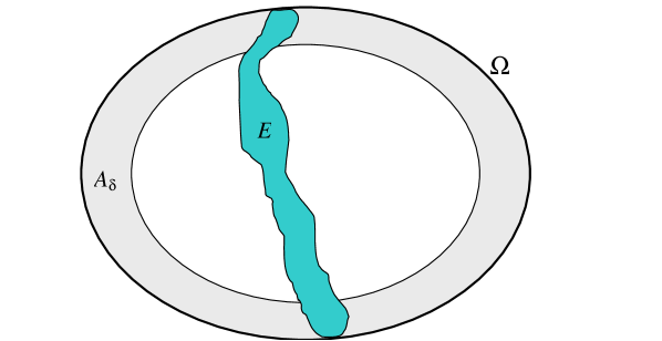
Figure 1.

Since $\left\|V_{\delta}^{+}\right\|_{L^{p}\left(\Omega\right)}$ can be made sufficiently small by the choice of $\delta>0$, the following boundary value problem has a unique positive solution:

$$\left\{\begin{array}[]{l}\Delta w+V_{\delta}w=0\ \text{in }\Omega\\ w=f\ \text{on }\partial\Omega,\end{array}\right.$$ (11)

for any positive continuous function $f$ on $\partial\Omega$. Denote by $q_{\delta}\left(x\right)$,$\ x\in\partial\Omega,$ the Poisson kernel of (11) at the source $x_{0}$. Letting $\delta\rightarrow 0$, we obtain that the solution of (11) converges to that of

$$\left\{\begin{array}[]{l}\Delta w-\frac{1}{N}w=0\ \text{in }\Omega\\ w=f\ \text{on }\partial\Omega.\end{array}\right.$$ (12)

Denoting by $q_{0}$ the Poisson kernel of (12) at the source $x_{0}$, we obtain that $q_{\delta}\searrow q_{0}$ on $\partial\Omega$ as $\delta\searrow 0$ and, moreover, the convergence is uniform.

Let $q$ be the Poisson kernel of the Laplace operator $\Delta$ in $\Omega$, as in the statement of the theorem. Since any solution of (12) is strictly subharmonic in $\Omega$, we obtain that $q_{0}<q$ on $\partial\Omega$. In particular, there is a constant $\eta>0$ depending only on $\Omega,N,x_{0}$ such that

$$q_{0}<\left(1-\eta\right)q\ \text{on }\partial\Omega.$$

Since the convergence $q_{\delta}\rightarrow q$ is uniform on $\partial\Omega$, we obtain that, for small enough $\delta$ (depending on $\Omega,N,x_{0}$),

$$q_{\delta}<\left(1-\eta/2\right)q\ \text{on\ }\partial\Omega.$$

Fix such $\delta$. Consequently, we obtain for the solution $w$ of (11) that

$$w\left(x_{0}\right)<\left(1-\eta/2\right)\int_{\partial\Omega}fqd\sigma.$$ (13)

Note that the function $W$ from (8) can be increased without violating (7). Define a new potential $W_{\delta}$ by

$$W_{\delta}=\left\{\begin{array}[]{l}N\ \ \text{in\ \ }A_{\delta}\cup E,\\ -\frac{1}{N}\ \ \text{in }\Omega\setminus A_{\delta}\setminus E.\end{array}\right.$$ (14)

Observe that, for any $p>1$

$$\left\|W_{\delta}^{+}\right\|_{L^{p}\left(\Omega\right)}^{p}\leq N^{p}\left(\mu\left(A_{\delta}\right)+\varepsilon\right),$$

so that by the choice of $\varepsilon$ and further reducing $\delta$ this norm can be made arbitrarily small. By a well-known fact (see [13]), if $\left\|\,W_{\delta}^{+}\right\|_{L^{p}\left(\Omega\right)}$ is sufficiently small, then the operator $-\Delta-$ $W_{\delta}$ in $\Omega$ with the Dirichlet boundary condition on $\partial\Omega$ is positive definite, provided $p=n/2$ for $n>2$ and $p>1$ for $n=2$.

So, we can assume that the operator $-\Delta-$ $W_{\delta}$ is positive definite. In particular, the following boundary value problem

$$\left\{\begin{array}[]{l}\Delta u+\,W_{\delta}u=0\ \text{in }\Omega\\ u|_{\partial\Omega}=v\end{array}\right.$$ (15)

has a unique positive solution $u$. Comparing this with (7) and using the maximum principle for the operator $\Delta+$ $W_{\delta}$, we obtain $u\geq v$ in $\Omega$. Since $u=v$ on $\partial\Omega$, the required inequality (9) will follow if we prove that

$$u\left(x_{0}\right)<\int_{\partial\Omega}uqd\sigma.$$ (16)

Set $\Omega_{\delta}=\Omega\setminus A_{\delta}$ and prove that

$$\sup_{\Omega_{\delta}}u\leq C\int_{\partial\Omega}ud\sigma,$$ (17)

for some constant $C$ that depends on $\Omega,N,\delta,n$. By choosing $\varepsilon$ and $\delta$ sufficiently small, the norm $\left\|W_{\delta}\right\|_{L^{p}}$ can be made arbitrarily small for any $p$. Hence, function $u$ satisfies the Harnack inequality

$$\sup_{\Omega_{\delta}}u\leq C\int_{\Omega_{\delta}}ud\mu$$ (18)

where $C$ depends on $\Omega,N,\delta$ (see [1], [7]). Let $h$ be the solution of the following boundary value problem

$$\left\{\begin{array}[]{l}-\Delta h-W_{\delta}h=1_{\Omega_{\delta}}\ \text{in }\Omega\\ h=0\ \text{on }\partial\Omega.\end{array}\right.$$

where $\Omega_{\delta}=\Omega\setminus A_{\delta}$. Since $\left\|W_{\delta}\right\|_{L^{q}}$ is bounded for any $q$, we obtain by the known a priori estimates, that

$$\left\|h\right\|_{W^{2,p}\left(\Omega\right)}\leq C\left\|1_{\Omega_{\delta}}\right\|_{L^{p}\left(\Omega\right)},$$

where $p>1$ is arbitrary and $C$ depends on $\Omega,N,\delta,p$ (see [10]). Choose $p>n$ so that by the Sobolev embedding

$$\left\|h\right\|_{C^{1}\left(\Omega\right)}\leq C\left\|h\right\|_{W^{2,p}\left(\Omega\right)}.$$

Since $\left\|1_{\Omega_{\delta}}\right\|_{L^{p}\left(\Omega\right)}$ is uniformly bounded, we obtain by combining the above estimates that

$$\left\|h\right\|_{C^{1}\left(\Omega\right)}\leq C,$$

with a constant $C$ depending on $\Omega,N,\delta,n.$

Multiplying the equation $-\Delta h-W_{\delta}h=1_{\Omega_{\delta}}\$by $u$ and integrating over $\Omega$, we obtain

$$\int_{\Omega_{\delta}}ud\mu=\int_{\partial\Omega}\frac{\partial h}{\partial\nu}u~{}d\sigma\leq C\int_{\partial\Omega}ud\sigma$$

which together with (18) implies (17).

Let $w$ be the solution (11) with the boundary condition $f=u$, that is,

$$\left\{\begin{array}[]{l}\Delta w+V_{\delta}w=0\ \text{in }\Omega\\ w=u\ \text{on }\partial\Omega.\end{array}\right.$$

Let us consider the difference

$$\varphi=u-w.$$

Clearly, we have in $\Omega$

$$\Delta\varphi+V_{\delta}\varphi=\left(\Delta u+V_{\delta}u\right)-\left(\Delta w+V_{\delta}w\right)=(V_{\delta}-\,W_{\delta})u$$

and $\varphi=0$ on $\partial\Omega$. Denoting by $G_{V_{\delta}}$ the Green function of the operator $-\Delta-V_{\delta}$ in $\Omega$ with the Dirichlet boundary condition, we obtain

$$\varphi\left(x_{0}\right)=\int_{\Omega}G_{V_{\delta}}\left(x_{0},y\right)\left(\,W_{\delta}-V_{\delta}\right)u\left(y\right)d\mu\left(y\right).$$

Since we are looking for an upper bound for $\varphi\left(x_{0}\right)$, we can restrict the integration to the domain $\left\{V_{\delta}\leq\,W_{\delta}\right\}$. By (14) and (10) we have

$$\left\{V_{\delta}\leq\,W_{\delta}\right\}=\left(\Omega\setminus A_{\delta}\right)\cap\left(A_{\delta}\cup E\right)=E\setminus A_{\delta}=:E^{\prime}$$

and, moreover, on $E^{\prime}$ we have

$$\,W_{\delta}-V_{\delta}=N+\frac{1}{N}<2N,$$

whence it follows that

$$\varphi\left(x_{0}\right)\leq 2N\int_{E^{\prime}}G_{V_{\delta}}\left(x_{0},y\right)u\left(y\right)d\mu\left(y\right).$$

Using (17) to estimate here $u\left(y\right)$, we obtain

$$\varphi\left(x_{0}\right)\leq 2NC\left(\int_{E^{\prime}}G_{V_{\delta}}\left(x_{0},y\right)d\mu\left(y\right)\right)\int_{\partial\Omega}ud\sigma$$

Since $\mu\left(E^{\prime}\right)\leq\varepsilon$ and the Green function $G_{V_{\delta}}\left(x_{0},\cdot\right)$ is integrable, we see that $\int_{E^{\prime}}G_{V_{\delta}}\left(x_{0},\cdot\right)d\mu$ can be made arbitrarily small by choosing $\varepsilon>0$ small enough. Choose $\varepsilon$ so small that

$$2NC\int_{E^{\prime}}G_{V_{\delta}}\left(x_{0},y\right)d\mu\left(y\right)<\eta/2\inf_{\partial\Omega}q,$$

which implies that

$$\varphi\left(x_{0}\right)<\eta/2\int_{\partial\Omega}uqd\sigma.$$

Since by (13)

$$w\left(x_{0}\right)<\left(1-\eta/2\right)\int_{\partial\Omega}uqd\sigma,$$

we obtain

$$u\left(x_{0}\right)=\varphi\left(x_{0}\right)+w\left(x_{0}\right)<\int_{\partial\Omega}uqd\sigma,$$

which was to be proved. ∎

Let $V_{\max}$ be a solution of the problem (4). Denote by $U$ the eigenspace of $-\Delta-V_{\max}$ associated with the eigenvalue $\lambda_{k}\left(V_{\max}\right)=0$ assuming that $N$ is sufficiently large.

Lemma 3.4.

Fix some $c>0$ and consider the set

$$F=\left\{V_{max}\leq-c\right\}.$$

Then, for any Lebesgue point $x\in F$, then there exists a non-negative function $q\in L^{\infty}\left(M\right)$ such that

1. $\int_{M}q\,d\mu=1$;

2. for any $u\in U\setminus\left\{0\right\}$ we have

   $$u^{2}(x)<\int_{M}u^{2}q\,d\mu.$$ (19)

Proof.

Set $V=V_{\max}$. Any function $u\in U$ satisfies $\Delta u+Vu=0,$ which implies by a simple calculation that the function $v=u^{2}$ satisfies

$$\Delta v+2Vv\geq 0.$$

Next, we apply Lemma 3.3 with $J=\max(2N,\frac{1}{2c})$. Choose $r$ so small that the density of the set $F$ in $B(x,r)$ is sufficiently close to $1$, namely,

$$\mu\left(F\cap B\left(x,r\right)\right)>\left(1-\varepsilon\right)\mu\left(B\left(x,r\right)\right),$$

where $\varepsilon=\varepsilon\left(J\right)$ is given in Lemma 3.3. Since $h\leq 2N\leq J$ in $B\left(x,r\right)$ and

$$\mu\left(\left\{h>-\frac{1}{J}\right\}\cap B\left(x,r\right)\right) \leq \mu\left(\left\{h>-2c\right\}\cap B\left(x,r\right)\right)$$

$$= \mu\left(\left\{V>-c\right\}\cap B\left(x,r\right)\right)$$

$$< \varepsilon\mu\left(B\left(x,r\right)\right),$$

all the hypotheses of Lemma 3.3 are satisfied. Let $q$ be the function that exists by Lemma 3.3 in some small ball $B\left(x,r\right).$ Extending $q$ by setting $q=0$ outside $B\left(x,r\right)$ we obtain a desirable function. ∎

3.3. Proof of main Lemma 3.1

We can now prove Lemma 3.1, that is, that $V_{\max}\geq 0$. Consider again the set

$$F=\left\{V_{max}\leq-c\right\},$$

where $c>0$. We want to show that, for any $c>0$,

$$\mu(F)=0,$$

which will imply the claim. Assume the contrary, that is $\mu(F)>0$ for some $c>0$. Denote by $F_{L}$ the set of Lebesgue points of $F$. For any $x\in F_{L}$ denote by $q_{x}$ the function $q$ that is given by Lemma 3.4. For $x\notin F_{L}$ set $q_{x}=\delta_{x}$. Then $x\mapsto q_{x}$ is a Markov kernel and, for all $x\in M$ and $u\in U$

$$u^{2}\left(x\right)\leq\int_{M}u^{2}q_{x}d\mu.$$ (20)

Denote by $\mathcal{M}$ the set of all probability measures on $M$. Define on $\mathcal{M}$ a partial order: $\nu_{1}\preceq\nu_{2}$ if and only if

$$\int_{M}u^{2}d\nu_{1}\leq\int_{M}u^{2}d\nu_{2}\ \text{for all }u\in U\setminus\left\{0\right\}.$$ (21)

Define $\nu_{0}\in\mathcal{M}$ by

$$d\nu_{0}=\frac{1}{\mu\left(F_{L}\right)}\mathbf{1}_{F_{L}}d\mu$$

and measure $\nu_{1}\in\mathcal{M}$ by

$$\nu_{1}=\int_{M}q_{x}d\nu_{0}\left(x\right).$$

Since $\nu_{0}\left(F_{L}\right)>0$, we obtain for any $u\in U\setminus\left\{0\right\}$ that

$$\int_{M}u^{2}d\nu_{1} = \int_{M}\left(\int_{M}u^{2}q_{x}d\mu\right)d\nu_{0}\left(x\right)$$ (22)

$$\geq \int_{F_{L}}\left(\int_{M}u^{2}q_{x}d\mu\right)d\nu_{0}\left(x\right)+\int_{M\setminus F_{L}}\left(\int_{M}u^{2}q_{x}d\mu\right)d\nu_{0}\left(x\right)$$

$$> \int_{F_{L}}u^{2}\left(x\right)d\nu_{0}\left(x\right)+\int_{M\setminus F_{L}}u^{2}\left(x\right)d\nu_{0}\left(x\right)$$

$$= \int_{M}u^{2}d\nu_{0}.$$

In particular, we have $\nu_{0}\preceq\nu_{1}$. Consider the following subset of $\mathcal{M}$:

$$\mathcal{M}_{1}=\left\{\nu\in\mathcal{M}:\nu\succeq\nu_{1}\right\}.$$

Let us prove that $\mathcal{M}_{1}$ has a maximal element. By Zorn’s Lemma, it suffices to show that any chain (=totally ordered subset) $\mathcal{C}$ of $\mathcal{M}_{1}$ has an upper bound in $\mathcal{M}_{1}$. It follows from $\dim U<\infty$ that there exists an increasing sequence $\left\{\nu_{i}\right\}_{i=1}^{\infty}$ of elements of $\mathcal{C}$ such that, for all $u\in U$,

$$\lim_{i\rightarrow\infty}\int_{M}u^{2}d\nu_{i}\rightarrow\sup_{\left\{\nu\in\mathcal{C}\right\}}\int_{M}u^{2}d\nu.$$

The sequence $\left\{\nu_{{}_{i}}\right\}_{i=1}^{\infty}$ of probability measures is $w^{\ast}$-compact. Without loss of generality we can assume that this sequence is $w^{\ast}$-convergent. It follows that the measure

$$\nu_{\mathcal{C}}=w^{\ast}\text{-}\lim\nu_{i}\in\mathcal{M}_{1}$$

is an upper bound for $\mathcal{C}$.

By Zorn’s Lemma, there exists a maximal element $\nu$ in $\mathcal{M}_{1}$. Note that the measure $\nu$ can be alternatively constructed by using a standard balayage procedure (see e.g. [3, Proposition 2.1, p. 250]). Consider first the measure $\nu^{\prime}$ defined by $\nu^{\prime}=\int_{M}q_{x}d\nu\left(x\right)$. It follows from (20) that for any $u\in U$

$$\int_{M}u^{2}d\nu^{\prime} = \int_{M}\left(\int_{M}u^{2}q_{x}d\mu\right)d\nu$$

$$\geq \int_{M}u^{2}d\nu,$$

that is, $\nu^{\prime}\succeq\nu$, in particular, $\nu^{\prime}\in\mathcal{M}_{1}$. Since $\nu$ is a maximal element in $\mathcal{M}_{1}$, it follows that $\nu^{\prime}=\nu$, which implies the identity

$$\int_{M}u^{2}d\nu=\int_{M}\left(\int_{M}u^{2}q_{x}d\mu\right)d\nu.$$ (23)

Now we can prove that $\nu\left(F_{L}\right)=0$. Assuming from the contrary that $\nu\left(F_{L}\right)>0$, we obtain, for any $u\in U\setminus\left\{0\right\}$.

$$\int_{M}u^{2}d\nu = \int_{M}\left(\int_{M}u^{2}q_{x}d\mu\right)d\nu\left(x\right)$$ (24)

$$\geq \int_{F_{L}}\left(\int_{M}u^{2}q_{x}d\mu\right)d\nu\left(x\right)+\int_{M\setminus F_{L}}\left(\int_{M}u^{2}q_{x}d\mu\right)d\nu\left(x\right)$$

$$> \int_{F_{L}}u^{2}\left(x\right)d\nu\left(x\right)+\int_{M\setminus F_{L}}u^{2}\left(x\right)d\nu\left(x\right)$$

$$= \int_{M}u^{2}d\nu,$$

which is a contradiction. Finally, it follows from (22) and $\nu\in\mathcal{M}_{1}$ that, for any $u\in U\setminus\left\{0\right\}$,

$$\int_{M}u^{2}d\nu_{0}<\int_{M}u^{2}d\nu.$$

Measure $\nu$ can be approximated in $w^{\ast}$-sense by measures with bounded densities sitting in $M\setminus F_{L}.$ Therefore, there exists a non-negative function $\varphi\in L^{\infty}\left(M\right)$ that vanishes on $F_{L}$ and such that

$$\int_{M}\varphi d\mu=1$$

and, for any $u\in U\setminus\left\{0\right\}$,

$$\int_{M}u^{2}\varphi_{0}d\mu<\int_{M}u^{2}\varphi d\mu$$ (25)

where $\varphi_{0}=\frac{1}{\mu\left(F_{L}\right)}\mathbf{1}_{F_{L}}$. Consider now the potential

$$V_{t}=V_{max}+t\varphi_{0}-t\varphi.$$

We have for all $t$

$$\int_{M}V_{t}d\mu=\int_{M}V_{\max}d\mu$$

and for $t\rightarrow 0$

$$\lambda_{k}(V_{t})=\lambda_{k}(V_{\max})-t\alpha+o(t),$$

where $\alpha$ is the minimal eigenvalue of the quadratic form

$$Q\left(u,u\right)=\int_{M}u^{2}\left(\varphi_{0}-\varphi\right)d\mu,$$

which by (25) is negative definite. Therefore, $\alpha<0$, which together with $\lambda_{k}\left(V_{\max}\right)=0$ implies that, for all small enough $t>0$

$$\lambda_{k}(V_{t})>0.$$

Finally, let us show that $\left|V_{t}\right|\leq N$ $\mathrm{a.e.}$ Indeed, on $F$ we have

$$V_{t}\leq-c+t\varphi_{0}<N$$

for small enough $t>0$, and on $M\setminus F_{L}$ we have

$$V_{t}\leq V_{\max}-t\varphi\leq V_{\max}\leq N.$$

Therefore, $V\leq N$ $\mathrm{a.e.}$ for small enough $t>0$. Similarly, we have on $F_{L}$

$$V_{t}\geq V_{\max}+t\varphi_{0}\geq V_{\max}\geq-N$$

and on $M\setminus F$

$$V_{t}\geq-c-t\varphi\geq-N$$

for small enough $t>0$, which implies that $\left|V_{t}\right|\leq N$ $\mathrm{a.e.}$ for small enough $t>0$.

Hence, we obtain that $V_{t}$ is a solution to our optimization problem (4), but it satisfies $\lambda_{k}(V_{t})>0$, which contradicts the optimality of $V_{t}$ by Lemma 2.2.

References

- [1]
- [1] Aizenman M., Simon B., Brownian motion and Harnack’s inequality for Schrödinger operators, Comm. Pure Appl. Math., 35 (1982) 203-271.
- [2] Birman M.Sh., Solomyak M.Z., Estimates for the number of negative eigenvalues of the Schrödinger operator and its generalizations, Advances in Soviet Math., 7 (1991) 1-55.
- [3] Bliedtner J., Hansen W., “Potential theory – an analytic and probabilistic approach to balayage”, Universitext, Springer, Berlin-Heidelberg-New York-Tokyo, 1986.
- [4] El Soufi, Ahmad, Isoperimetric inequalities for the eigenvalues of natural Schrödinger operators on surfaces, Indiana Univ. Math. J., 58 (2009) no.1, 335-349.
- [5] Grigor’yan A., Nadirashvili N., Negative eigenvalues of two-dimensional Schr dinger equations, arXiv:1112.4986
- [6] Grigor’yan A., Netrusov Yu., Yau S.-T., Eigenvalues of elliptic operators and geometric applications, in: “Eigenvalues of Laplacians and other geometric operators”, Surveys in Differential Geometry IX, (2004) 147-218.
- [7] Hansen W., Harnack inequalities for Schrödinger operators, Ann. Scuola Norm. Sup. Pisa, 28 (1999) 413-470.
- [8] Harrell II, E.M, On the second eigenvalue of the Laplace operator penalized by curvature, Diff. Geom. Appl., 6 (1996) 397-400.
- [9] Kato T., “Perturbation theory for linear operators”, Springer, 1995.
- [10] Ladyzenskaja O.A., V.A. Solonnikov, Ural’ceva N.N., “Linear and quasilinear equations of parabolic type”, Providence, Rhode Island, 1968.
- [11] Li P., Yau S.-T., On the Schrödinger equation and the eigenvalue problem, Comm. Math. Phys., 88 (1983) 309–318.
- [12] Lieb E.H., The number of bound states of one-body Schrödinger operators and the Weyl problem, Proc. Sym. Pure Math., 36 (1980) 241-252.
- [13] Lieb E.H., Loss M., “Analysis”, AMS, 2001.
- [14] Nadirashvili N., Sire Y., Conformal spectrum and harmonic maps, arXiv:1007.3104
- [15] Yang P., Yau S.-T., Eigenvalues of the Laplacian of compact Riemann surfaces and minimal submanifolds, Ann. Scuola Norm. Sup. Pisa Cl. Sci. (4), 7 (1980) 55-63.