Block-Structured Supermarket Models

Abstract

Supermarket models are a class of parallel queueing networks with an adaptive control scheme that play a key role in the study of resource management of, such as, computer networks, manufacturing systems and transportation networks. When the arrival processes are non-Poisson and the service times are non-exponential, analysis of such a supermarket model is always limited, interesting, and challenging.

This paper describes a supermarket model with non-Poisson inputs: Markovian Arrival Processes (MAPs) and with non-exponential service times: Phase-type (PH) distributions, and provides a generalized matrix-analytic method which is first combined with the operator semigroup and the mean-field limit. When discussing such a more general supermarket model, this paper makes some new results and advances as follows: (1) Providing a detailed probability analysis for setting up an infinite-dimensional system of differential vector equations satisfied by the expected fraction vector, where the invariance of environment factors is given as an important result. (2) Introducing the phase-type structure to the operator semigroup and to the mean-field limit, and a Lipschitz condition can be obtained by means of a unified matrix-differential algorithm. (3) The matrix-analytic method is used to compute the fixed point which leads to performance computation of this system. Finally, we use some numerical examples to illustrate how the performance measures of this supermarket model depend on the non-Poisson inputs and on the non-exponential service times. Thus the results of this paper give new highlight on understanding influence of non-Poisson inputs and of non-exponential service times on performance measures of more general supermarket models.

Keywords: Randomized load balancing; Supermarket model; Matrix-analytic method; Operator semigroup; Mean-field limit; Markovian arrival processes (MAP); Phase-type (PH) distribution; Invariance of environment factors; Doubly exponential tail; $RG$-factorization.

1 Introduction

Supermarket models are a class of parallel queueing networks with an adaptive control scheme that play a key role in the study of resource management of, such as computer networks (e.g., see the dynamic randomized load balancing), manufacturing systems and transportation networks. Since a simple supermarket model was discussed by Mitzenmacher [23], Vvedenskaya et al [32] and Turner [30] through queueing theory as well as Markov processes, subsequent papers have been published on this theme, among which, see, Vvedenskaya and Suhov [33], Jacquet and Vvedenskaya [8], Jacquet et al [9], Mitzenmacher [24], Graham [5, 6, 7], Mitzenmacher et al [25], Vvedenskaya and Suhov [34], Luczak and Norris [20], Luczak and McDiarmid [18, 19], Bramson et al [1, 2, 3], Li et al [17], Li [13] and Li et al [15]. For the fast Jackson networks (or the supermarket networks), readers may refer to Martin and Suhov [22], Martin [21] and Suhov and Vvedenskaya [29].

The available results of the supermarket models with non-exponential service times are still few in the literature. Important examples include an approximate method of integral equations by Vvedenskaya and Suhov [33], the Erlang service times by Mitzenmacher [24] and Mitzenmacher et al [25], the PH service times by Li et al [17] and Li and Lui [16], and the ansatz-based modularized program for the general service times by Bramson et al [1, 2, 3].

Little work has been done on the analysis of the supermarket models with non-Poisson inputs, which are more difficult and challenging due to the higher complexity of that $N$ arrival processes are superposed. Li and Lui [16] and Li [12] used the superposition of $N$ MAP inputs to study the infinite-dimensional Markov processes of supermarket modeling type. Comparing with the results given in Li and Lui [16] and Li [12], this paper provides more necessary phase-level probability analysis in setting up the infinite-dimensional system of differential vector equations, which leads some new results and methodologies in the study of block-structured supermarket models. Note that the PH distributions constitute a versatile class of distributions that can approximate arbitrarily closely any probability distribution defined on the nonnegative real line, and the MAPs are a broad class of renewal or non-renewal point processes that can approximate arbitrarily closely any stochastic counting process (e.g., see Neuts [27, 28] and Li [11] for more details), thus the results of this paper are a key advance of those given in Mitzenmacher [23] and Vvedenskaya et al [32] under the Poisson and exponential setting.

The main contributions of this paper are threefold. The first one is to use the MAP inputs and the PH service times to describe a more general supermarket model with non-Poisson inputs and with non-exponential service times. Based on the phase structure, we define the random fraction vector and construct an infinite-dimensional Markov process, which expresses the state of this supermarket model by means of an infinite-dimensional Markov process. Furthermore, we set up an infinite-dimensional system of differential vector equations satisfied by the expected fraction vector through a detailed probability analysis. To that end, we obtain an important result: The invariance of environment factors, which is a key for being able to simplify the differential equations in a vector form. Based on the differential vector equations, we can provide a generalized matrix-analytic method to investigate more general supermarket models with non-Poisson inputs and with non-exponential service times. The second contribution of this paper is to provide phase-structured expression for the operator semigroup with respect to the MAP inputs and to the PH service times, and use the operator semigroup to provide the mean-field limit for the sequence of Markov processes who asymptotically approaches a single trajectory identified by the unique and global solution to the infinite-dimensional system of limiting differential vector equations. To prove the existence and uniqueness of solution through the Picard approximation, we provide a unified computational method for establishing a Lipschitz condition, which is crucial in all the rigor proofs involved. The third contribution of this paper is to provide an effective matrix-analytic method both for computing the fixed point and for analyzing performance measures of this supermarket model. Furthermore, we use some numerical examples to indicate how the performance measures of this supermarket model depend on the non-Poisson MAP inputs and on the non-exponential PH service times. Therefore, the results of this paper gives new highlight on understanding performance analysis and nonlinear Markov processes for more general supermarket models with non-Poisson inputs and non-exponential service times.

The remainder of this paper is organized as follows. In Section 2, we first introduce a new MAP whose transition rates are controlled by the number of servers in the system. Then we describe a more general supermarket model of $N$ identical servers with MAP inputs and PH service times. In Section 3, we define a random fraction vector and construct an infinite-dimensional Markov process, which expresses the state of this supermarket model. In Section 4, we set up an infinite-dimensional system of differential vector equations satisfied by the expected fraction vector through a detailed probability analysis, and establish an important result: The invariance of environment factors. In Section 5, we show that the mean-field limit for the sequence of Markov processes who asymptotically approaches a single trajectory identified by the unique and global solution to the infinite-dimensional system of limiting differential vector equations. To prove the existence and uniqueness of the solution, we provide a unified matrix-differential algorithm for establishing the Lipschitz condition. In Section 6, we first discuss the stability of this supermarket model in terms of a coupling method. Then we provide a generalized matrix-analytic method for computing the fixed point whose doubly exponential solution and phase-structured tail are obtained. Finally, we discuss some useful limits of the fraction vector $\mathbf{u}^{\left(N\right)}\left(t\right)$ as $N\rightarrow\infty$ and $t\rightarrow+\infty$. In Section 7, we provide two performance measures of this supermarket model, and use some numerical examples to indicate how the performance measures of this system depend on the non-Poisson MAP inputs and on the non-exponential PH service times. Some concluding remarks are given in Section 8. Finally, Appendices A and C are respectively designed for the proofs of Theorems 1 and 3, and Appendix B contains the proof of Theorem 2, where the mean-field limit of the sequence of Markov processes in this supermarket model is given a detailed analysis through the operator semigroup.

2 Supermarket Model Description

In this section, we first introduce a new MAP whose transition rates are controlled by the number of servers in the system. Then we describe a more general supermarket model of $N$ identical servers with MAP inputs and PH service times.

2.1 A new Markovian arrival process

Based on Chapter 5 in Neuts [28], the MAP is a bivariate Markov process $\left\{\left(N(t),J(t)\right):t\geq 0\right\}$ with state space $S=\left\{1,2,3,\ldots\right\}\times\left\{1,2,\ldots,m_{A}\right\}$, where $\left\{N(t):t\geq 0\right\}$ is a counting process of arrivals and $\left\{J(t):t\geq 0\right\}$ is a Markov environment process. When $J(t)=i$, if the random environment shall go to state $j$ in the next time, then the counting process $\left\{N(t):t\geq 0\right\}$ is a Poisson process with arrival rate $d_{i,j}$ for $1\leq i,j\leq m_{A}$. The matrix $D$ with elements $d_{i,j}$ satisfies $D\gvertneqq 0$. The matrix $C$ with elements $c_{i,j}$ has negative diagonal elements and nonnegative off-diagonal elements, and the matrix $C$ is invertible, where $c_{i,j}$ is a state transition rate of the Markov chain $\left\{J(t):t\geq 0\right\}$ from state $i$ to state $j$ for $i\neq j$. The matrix $Q=C+D$ is the infinitesimal generator of an irreducible Markov chain. We assume that $Qe=0$, where $e$ is a column vector of ones with a suitable size. Hence, we have

$$c_{i,i}=-\left[\sum\limits_{j=1}^{m_{A}}d_{i,j}+\sum\limits_{j\neq i}^{m_{A}}c_{i,j}\right].$$

Let

$$\mathbb{C}=\left(\begin{array}[c]{cccc}-\sum\limits_{j\neq 1}^{m_{A}}c_{1,j}&c_{1,2}&\cdots&c_{1,m_{A}}\\ c_{2,1}&-\sum\limits_{j\neq 2}^{m_{A}}c_{2,j}&\cdots&c_{2,m_{A}}\\ \vdots&\vdots&\ddots&\vdots\\ c_{m_{A},1}&c_{m_{A},2}&\cdots&-\sum\limits_{j\neq m_{A}}^{m_{A}}c_{m_{A},j}\end{array}\right),$$

$$C(N)=\mathbb{C}-N\text{diag}(De),$$

$$D(N)=ND,$$

where

$$\text{diag}(De)=\text{diag}\left(\sum\limits_{j=1}^{m_{A}}d_{1,j},\sum\limits_{j=1}^{m_{A}}d_{2,j},\ldots,\sum\limits_{j=1}^{m_{A}}d_{m_{A},j}\right).$$

Then

$$Q\left(N\right)=C(N)+D(N)=\left[\mathbb{C}-N\text{diag}(De)\right]+ND$$

is obviously the infinitesimal generator of an irreducible Markov chain with $m_{A}$ states. Thus $\left(C(N),D(N)\right)$ is the irreducible matrix descriptor of a new MAP of order $m_{A}$. Note that the new MAP is non-Poisson and may also be non-renewal, and its arrival rate at each environment state is controlled by the number $N$ of servers in the system.

Note that

$$Q\left(N\right)e=\left[\mathbb{C}-N\text{diag}(De)\right]e+NDe=0,$$

the Markov chain $Q\left(N\right)$ with $m_{A}$ states is irreducible and positive recurrent. Let $\omega_{N}$ be the stationary probability vector of the Markov chain $Q\left(N\right)$. Then $\omega_{N}$ depends on the number $N\geq 1$, and the stationary arrival rate of the MAP is given by $N\lambda_{N}=N\omega_{N}De$.

2.2 Model description

Based on the new MAP, we describe a more general supermarket model of $N$ identical servers with MAP inputs and PH service times as follows:

Non-Poisson inputs: Customers arrive at this system as the MAP of irreducible matrix descriptor $\left(C\left(N\right),D\left(N\right)\right)$ of size $m_{A}$, whose stationary arrival rate is given by $N\lambda_{N}=N\omega_{N}De$.

Non-exponential service times: The service times of each server are i.i.d. and are of phase type with an irreducible representation $\left(\alpha,T\right)$ of order $m_{B}$, where the row vector $\alpha$ is a probability vector whose $j$th entry is the probability that a service begins in phase $j$ for $1\leq j\leq m_{B}$; $T$ is a matrix of size $m_{B}$ whose $\left(i,j\right)^{\text{th}}$ entry is denoted by $t_{i,j}$ with $t_{i,i}<0$ for $1\leq i\leq m_{B}$, and $t_{i,j}\geq 0$ for $i\neq j$. Let $T^{0}=-Te=\left(t_{1}^{0},t_{2}^{0},\ldots,t_{m_{B}}^{0}\right)^{\text{T}}\gvertneqq 0$, where “$A^{T}$” denotes the transpose of matrix (or vector) $A$. When a PH service time is in phase $i$, the transition rate from phase $i$ to phase $j$ is $t_{i,j}$, the service completion rate is $t_{i}^{0}$, and the output rate from phase $i$ is $\mu_{i}=-t_{i,i}$. At the same time, the mean of the PH service time is given by $1/\mu=-\alpha T^{-1}e$.

Arrival and service disciplines: Each arriving customer chooses $d\geq 1$ servers independently and uniformly at random from the $N$ identical servers, and waits for its service at the server which currently contains the fewest number of customers. If there is a tie, servers with the fewest number of customers will be chosen randomly. All customers in any server will be served in the FCFS manner. Figure 1 gives a physical interpretation for this supermarket model.

Figure 1: The supermarket model with MAP inputs and PH service times

Remark 1

The block-structured supermarket models can have many practical applications to, such as, computer networks and manufacturing system, where it is a key to introduce the PH service times and the MAP inputs to such a practical model, because the PH distributions contain many useful distributions such as exponential, hyper-exponential and Erlang distributions; while the MAPs include, for example, Poisson process, PH-renewal processes, and Markovian modulated Poisson processes (MMPPs). Note that the probability distributions and stochastic point processes have extensively been used in most practical stochastic modeling. On the other hand, in many practical applications, the block-structured supermarket model is an important queueing model to analyze the relation between the system performance and the job routing rule, and it can also help to design reasonable architecture to improve the performance and to balance the load.

3 An Infinite-Dimensional Markov Process

In this section, we first define the random fraction vector of this supermarket model. Then we use the the random fraction vector to construct an infinite-dimensional Markov process, which describes the state of this supermarket model.

For this supermarket model, let $n_{k;i,j}^{\left(N\right)}\left(t\right)$ be the number of servers with at least $k$ customers (note that the serving customer is also taken into account), and with the MAP be in phase $i$ and the PH service time be in phase $j$ at time $t\geq 0$. Clearly, $0\leq n_{0;i}^{\left(N\right)}\left(t\right)\leq N$ and $0\leq n_{k;i,j}^{\left(N\right)}\left(t\right)\leq N$ for $k\geq 1$, $1\leq i\leq m_{A}$ and $1\leq j\leq m_{B}$. Let

$$U_{0;i}^{\left(N\right)}\left(t\right)=\frac{n_{0;i}^{\left(N\right)}\left(t\right)}{N},\text{ \ }1\leq i\leq m_{A},$$

and for $k\geq 1$

$$U_{k;i,j}^{\left(N\right)}\left(t\right)=\frac{n_{k;i,j}^{\left(N\right)}\left(t\right)}{N},\text{ \ }1\leq i\leq m_{A},1\leq j\leq m_{B}.$$

Then $U_{k;i,j}^{\left(N\right)}\left(t\right)$ is the fraction of servers with at least $k$ customers, and with the MAP be in phase $i$ and the PH service time be in phase $j$ at time $t$. Using the lexicographic order we write

$$U_{0}^{\left(N\right)}\left(t\right)=\left(U_{0;1}^{\left(N\right)}\left(t\right),U_{0;2}^{\left(N\right)}\left(t\right),\ldots,U_{0;m_{A}}^{\left(N\right)}\left(t\right)\right)\text{ }$$

for $k\geq 1$

$$U_{k}^{\left(N\right)}\left(t\right)= \left(U_{k;1,1}^{\left(N\right)}\left(t\right),U_{k;1,2}^{\left(N\right)}\left(t\right),\ldots,U_{k;1,m_{B}}^{\left(N\right)}\left(t\right);\ldots;\right.$$

$$\left.U_{k;m_{A},1}^{\left(N\right)}\left(t\right),U_{k;m_{A},2}^{\left(N\right)}\left(t\right),\ldots,U_{k;m_{A},m_{B}}^{\left(N\right)}\left(t\right)\right),$$

and

$$U^{\left(N\right)}\left(t\right)=\left(U_{0}^{\left(N\right)}\left(t\right),U_{1}^{\left(N\right)}\left(t\right),U_{2}^{\left(N\right)}\left(t\right),\ldots\right).$$ (1)

Let $a=\left(a_{1},a_{2},a_{3},\ldots\right)$ and $b=\left(b_{1},b_{2},b_{3},\ldots\right)$. We write $a<b$ if $a_{k}<b_{k}$ for some $k\geq 1$; $a\leq b$ if $a_{k}\leq b_{k}$ for every $k\geq 1$.

For a fixed quaternary array $\left(t,N,i,j\right)$ with $t\geq 0,N\in\left\{1,2,3,\ldots\right\},i\in\left\{1,2,\ldots,m_{A}\right\}$ and $j\in\left\{1,2,\ldots,m_{B}\right\}$, it is easy to see from the stochastic order that $n_{k;i,j}^{\left(N\right)}\left(t\right)\geq n_{k+1;i,j}^{\left(N\right)}\left(t\right)$ for $k\geq 1$. This gives

$$U_{1}^{\left(N\right)}\left(t\right)\geq U_{2}^{\left(N\right)}\left(t\right)\geq U_{3}^{\left(N\right)}\left(t\right)\cdots\geq 0$$ (2)

and

$$1=U_{0}^{\left(N\right)}\left(t\right)e\geq U_{1}^{\left(N\right)}\left(t\right)e\geq U_{2}^{\left(N\right)}\left(t\right)e\geq U_{3}^{\left(N\right)}\left(t\right)e\geq\cdots\geq 0.$$ (3)

Note that the state of this supermarket model is described as the random fraction vector $U^{\left(N\right)}\left(t\right)$ for $t\geq 0$, and $\left\{U^{\left(N\right)}\left(t\right),t\geq 0\right\}$ is a stochastic vector process for each $N=1,2,\ldots$. Since the arrival process to this supermarket model is the MAP and the service times in each server are of phase type, $\left\{U^{\left(N\right)}\left(t\right),t\geq 0\right\}$ is an infinite-dimensional Markov process whose state space is given by

$$\widetilde{\Omega}_{N}= \left\{\left(h_{0}^{\left(N\right)},h_{1}^{\left(N\right)},h_{2}^{\left(N\right)}\ldots\right):h_{0}^{\left(N\right)}\text{ is a probability vector of size }m_{A},\right.$$

$$\left.h_{1}^{\left(N\right)}\geq h_{2}^{\left(N\right)}\geq h_{3}^{\left(N\right)}\geq\cdots\geq 0,h_{k}^{\left(N\right)}\text{ is a row vector of size }m_{A}m_{B}\text{ for }k\geq 1,\right.$$

$$\left.1=h_{0}^{\left(N\right)}e\geq h_{1}^{\left(N\right)}e\geq h_{2}^{\left(N\right)}e\geq\cdots\geq 0,\right.$$

$$\left.\text{and \ }Nh_{k}^{\left(N\right)}\text{ \ is a row vector of nonnegative integers for }k\geq 0\right\},$$ (4)

We write

$$u_{0;i}^{\left(N\right)}\left(t\right)=E\left[U_{0;i}^{\left(N\right)}\left(t\right)\right]$$

and for $k\geq 1$

$$u_{k;i,j}^{\left(N\right)}\left(t\right)=E\left[U_{k;i,j}^{\left(N\right)}\left(t\right)\right].$$

Using the lexicographic order we write

$$u_{0}^{\left(N\right)}\left(t\right)=\left(u_{0;1}^{\left(N\right)}\left(t\right),u_{0;2}^{\left(N\right)}\left(t\right),\ldots,u_{0;m_{A}}^{\left(N\right)}\left(t\right)\right)$$

and for $k\geq 1$

$$u_{k}^{\left(N\right)}\left(t\right)= \left(u_{k;1,1}^{\left(N\right)}\left(t\right),u_{k;1,2}^{\left(N\right)}\left(t\right),\ldots,u_{k;1,m_{B}}^{\left(N\right)}\left(t\right);\ldots;\right.$$

$$\left.u_{k;m_{A},1}^{\left(N\right)}\left(t\right),u_{k;m_{A},2}^{\left(N\right)}\left(t\right),\ldots,u_{k;m_{A},m_{B}}^{\left(N\right)}\left(t\right)\right),$$

$$\mathbf{u}^{\left(N\right)}\left(t\right)=\left(u_{0}^{\left(N\right)}\left(t\right),u_{1}^{\left(N\right)}\left(t\right),u_{2}^{\left(N\right)}\left(t\right),\ldots\right).$$

It is easy to see from Equations (2) and (3) that

$$u_{1}^{\left(N\right)}\left(t\right)\geq u_{2}^{\left(N\right)}\left(t\right)\geq u_{3}^{\left(N\right)}\left(t\right)\cdots\geq 0$$ (5)

and

$$1=u_{0}^{\left(N\right)}\left(t\right)e\geq u_{1}^{\left(N\right)}\left(t\right)e\geq u_{2}^{\left(N\right)}\left(t\right)e\geq\cdots\geq 0.$$ (6)

In the remainder of this section, for convenience of readers, it is necessary to explain the structure of this long paper which is outlined as follows. Part one: The limit of the sequence of Markov processes. It is seen from (1) and (4) that we need to deal with the limit of the sequence $\left\{U^{\left(N\right)}\left(t\right)\right\}$ of infinite-dimensional Markov processes. This is organized in Appendix B by means of the convergence theorems of operator semigroups, e.g., see Ethier and Kurtz [4] for more details. Part two: The existence and uniqueness of the solution. As seen from Theorem 2 and (32), we need to study the two means $E\left[U^{\left(N\right)}\left(t\right)\right]$ and $E\left[U\left(t\right)\right]=\lim_{N\rightarrow\infty}E\left[U^{\left(N\right)}\left(t\right)\right]$, or $\mathbf{u}^{\left(N\right)}\left(t\right)$ and $\mathbf{u}\left(t\right)=\lim_{N\rightarrow\infty}\mathbf{u}^{\left(N\right)}\left(t\right)$. To that end, Section 4 sets up the system of differential vector equations satisfied by $\mathbf{u}^{\left(N\right)}\left(t\right)$, while Section 5 provides a unified matrix-differential algorithm for establishing the Lipschitz condition, which is a key in proving the existence and uniqueness of the solution to the limiting system of differential vector equations satisfied by $\mathbf{u}\left(t\right)$ through the Picard approximation. Part three: Computation of the fixed point and performance analysis. Section 6 discusses the stability of this supermarket model in terms of a coupling method, and provide an effective matrix-analytic method for computing the fixed point. Section 7 analyzes the performance of this supermarket model by means of some numerical examples.

4 The System of Differential Vector Equations

In this section, we set up an infinite-dimensional system of differential vector equations satisfied by the expected fraction vector through a detailed probability analysis. Specifically, we obtain an important result: The invariance of environment factors, which is a key to rewriting the differential equations as a simple vector form.

To derive the system of differential vector equations, we first discuss an example with the number $k\geq 2$ of customers through the following three steps:

Step one: Analysis of the Arrival Processes

In this supermarket model of $N$ identical servers, we need to determine the change in the expected number of servers with at least $k$ customers over a small time period $\left[0,\text{d}t\right)$. When the MAP environment process $\left\{J\left(t\right):t\geq 0\right\}$ jumps form state $l$ to state $i$ for $1\leq l,i\leq m_{A}$ and the PH service environment process $\left\{I\left(t\right):t\geq 0\right\}$ sojourns at state $j$ for $1\leq j\leq m_{B}$, one arrival occurs in a small time period $\left[0,\text{d}t\right)$. In this case, the rate that any arriving customer selects $d$ servers with at least $k-1$ customers at random and joins the shortest one with $k-1$ customers, is given by

$$\sum_{l=1}^{m_{A}}\left[u_{k-1;l,j}^{\left(N\right)}\left(t\right)d_{l,i}-u_{k;i,j}^{\left(N\right)}\left(t\right)\left(d_{i,1},d_{i,2},\ldots,d_{i,m_{A}}\right)e\right]$$

$$\times L_{k;l}^{\left(N\right)}\left(u_{k-1}\left(t\right),u_{k}\left(t\right)\right)N\text{d}t,$$ (7)

where

$$L_{k;l}^{\left(N\right)}\left(u_{k-1}\left(t\right),u_{k}\left(t\right)\right)=\sum_{m=1}^{d}C_{d}^{m}\left\{\sum_{j=1}^{m_{B}}\left[u_{k-1;l,j}^{(N)}\left(t\right)-u_{k;l,j}^{(N)}\left(t\right)\right]\right\}^{m-1}\left\{\sum_{j=1}^{m_{B}}\left[u_{k;l,j}^{(N)}\left(t\right)\right]\right\}^{d-m}$$

$$+\sum_{m=1}^{d-1}C_{d}^{m}\left\{\sum_{j=1}^{m_{B}}\left[u_{k-1;l,j}^{(N)}\left(t\right)-u_{k;l,j}^{(N)}\left(t\right)\right]\right\}^{m-1}\sum_{\begin{subarray}{c}r_{1}+r_{2}+\cdots+r_{m_{A}}=d-m\\ \sum_{i\neq l}^{m_{A}}r_{i}\geq 1\\ 0\leq r_{j}\leq d-m,1\leq j\leq m_{A}\end{subarray}}\left(\begin{array}[c]{c}d-m\\ r_{1},r_{2},\ldots,r_{m_{A}}\end{array}\right)$$

$$\times\prod_{i=1}^{m_{A}}\left\{\sum_{j=1}^{m_{B}}\left[u_{k;i,j}^{(N)}\left(t\right)\right]\right\}^{r_{i}}+\sum_{m=2}^{d}C_{d}^{m}\sum_{m_{1}=1}^{m-1}\frac{m_{1}}{m}C_{m}^{m_{1}}\left\{\sum_{j=1}^{m_{B}}\left[u_{k-1;l,j}^{(N)}\left(t\right)-u_{k;l,j}^{(N)}\left(t\right)\right]\right\}^{m_{1}-1}$$

$$\times\sum_{\begin{subarray}{c}n_{1}+n_{2}+\cdots+n_{m_{A}}=m-m_{1}\\ \sum_{i\neq l}^{m_{A}}n_{i}\geq 1\\ 0\leq n_{j}\leq m-m_{1},1\leq j\leq m_{A}\end{subarray}}\left(\begin{array}[c]{c}m-m_{1}\\ n_{1},n_{2},\ldots,n_{m_{A}}\end{array}\right)\prod_{i=1}^{m_{A}}\left\{\sum_{j=1}^{m_{B}}\left[u_{k-1;i,j}^{(N)}\left(t\right)-u_{k;i,j}^{(N)}\left(t\right)\right]\right\}^{n_{i}}$$ (10)

$$\times\sum_{\begin{subarray}{c}r_{1}+r_{2}+\cdots+r_{m_{A}}=d-m\\ 0\leq r_{j}\leq d-m,1\leq j\leq m_{A}\end{subarray}}\left(\begin{array}[c]{c}d-m\\ r_{1},r_{2},\ldots,r_{m_{A}}\end{array}\right)\prod_{i=1}^{m_{A}}\left\{\sum_{j=1}^{m_{B}}\left[u_{k;i,j}^{(N)}\left(t\right)\right]\right\}^{r_{i}}.$$ (13)

Note that $\left[u_{k-1;l,j}^{\left(N\right)}\left(t\right)d_{l,i}-u_{k;i,j}^{\left(N\right)}\left(t\right)\left(d_{i,1},d_{i,2},\ldots,d_{i,m_{A}}\right)e\right]$ is the rate that any arriving customer joins one server with the shortest queue length $k-1$, where the MAP goes to phase $i$ from phase $l$, and the PH service time is in phase $j$.

Now, we provide a detailed interpretation for how to derive (13) through a set decomposition of all possible events given in Figure 2, where each of the $d$ selected servers has at least $k-1$ customers, the MAP arrival environment is in phase $i$ or $l$, and the PH service environment is in phase $j$. Hence, the probability that any arriving customer selects $d$ servers with at least $k-1$ customers at random and joins a server with the shortest queue length $k-1$ and with the MAP phase $i$ or $l$ is determined by means of Figure 2 through the following three parts:

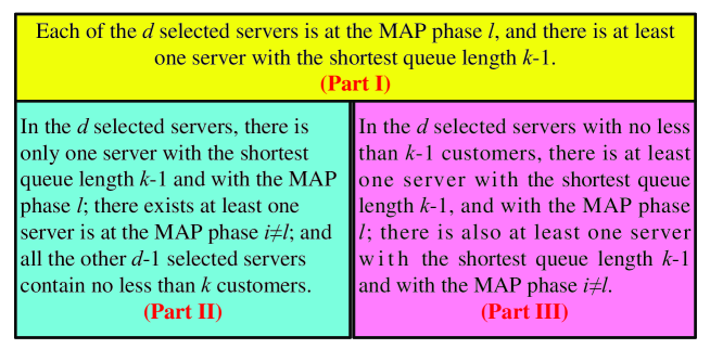
Figure 2: A set decomposition of all possible events

Part I: The probability that any arriving customer joins a server with the shortest queue length $k-1$ and with the MAP phase $l$, and the queue lengths of the other selected $d-1$ servers are not shorter than $k-1$, is given by

$$\sum_{m=1}^{d}C_{d}^{m}\left\{\sum_{j=1}^{m_{B}}\left[u_{k-1;l,j}^{(N)}\left(t\right)-u_{k;l,j}^{(N)}\left(t\right)\right]\right\}^{m-1}\left\{\sum_{j=1}^{m_{B}}\left[u_{k;l,j}^{(N)}\left(t\right)\right]\right\}^{d-m},$$

where $C_{d}^{m}=d!/\left[m!\left(d-m\right)!\right]$ is a binomial coefficient, and

$$\left\{\sum_{j=1}^{m_{B}}\left[u_{k-1;l,j}^{(N)}\left(t\right)-u_{k;l,j}^{(N)}\left(t\right)\right]\right\}^{m-1}$$

is the probability that any arriving customer who can only choose one server makes $m-1$ independent selections during the $m-1$ servers with the queue length $k-1$ and with the MAP phase $l$ at time $t$; while $\left\{\sum_{j=1}^{m_{B}}\left[u_{k;l,j}^{(N)}\left(t\right)\right]\right\}^{d-m}$ is the probability that there are $d-m$ servers whose queue lengths are not shorter than $k$ and with the MAP phase $l$.

Part II: The probability that any arriving customer joins a server with the shortest queue length $k-1$ and with the MAP phase $l$; and the queue lengths of the other selected $d-1$ servers are not shorter than $k-1$, and there exist at least one server with no less than $k$ customers and with the MAP phase $i\neq l$, is given by

$$\sum_{m=1}^{d-1}C_{d}^{m}\left\{\sum_{j=1}^{m_{B}}\left[u_{k-1;l,j}^{(N)}\left(t\right)-u_{k;l,j}^{(N)}\left(t\right)\right]\right\}^{m-1}$$

$$\times\sum_{\begin{subarray}{c}r_{1}+r_{2}+\cdots+r_{m_{A}}=d-m\\ \sum_{i\neq l}^{m_{A}}r_{i}\geq 1\\ 0\leq r_{j}\leq d-m,1\leq j\leq m_{A}\end{subarray}}\left(\begin{array}[c]{c}d-m\\ r_{1},r_{2},\ldots,r_{m_{A}}\end{array}\right)\prod_{i=1}^{m_{A}}\left\{\sum_{j=1}^{m_{B}}\left[u_{k;i,j}^{(N)}\left(t\right)\right]\right\}^{r_{i}},$$

where when $r_{1}+r_{2}+\cdots+r_{m_{A}}=n$, $\left(\begin{array}[c]{c}n\\ r_{1},r_{2},\ldots,r_{m_{A}}\end{array}\right)=\dfrac{n}{\prod\nolimits_{i=1}^{m_{A}}r_{i}!}$ is a multinomial coefficient.

Part III: If there are $m$ selected servers with the shortest queue length $k-1$ where there are $m_{1}\$servers with the MAP phase $l$ and $m-m_{1}$ servers with the MAP phases $i\neq l$, then the probability that any arriving customer joins a server with the shortest queue length $k-1$ and with the MAP phase $l$ is equal to $m_{1}/m$. In this case, the probability that any arriving customer joins a server with the shortest queue length $k-1$ and with the MAP phase $l$, the queue lengths of the other selected $d-1$ servers are not shorter than $k-1$, is given by

$$\sum_{m=2}^{d}C_{d}^{m}\sum_{m_{1}=1}^{m-1}\frac{m_{1}}{m}C_{m}^{m_{1}}\left\{\sum_{j=1}^{m_{B}}\left[u_{k-1;l,j}^{(N)}\left(t\right)-u_{k;l,j}^{(N)}\left(t\right)\right]\right\}^{m_{1}-1}$$

$$\times\sum_{\begin{subarray}{c}n_{1}+n_{2}+\cdots+n_{m_{A}}=m-m_{1}\\ \sum_{i\neq l}^{m_{A}}n_{i}\geq 1\\ 0\leq n_{j}\leq m-m_{1},1\leq j\leq m_{A}\end{subarray}}\left(\begin{array}[c]{c}m-m_{1}\\ n_{1},n_{2},\ldots,n_{m_{A}}\end{array}\right)\prod_{i=1}^{m_{A}}\left\{\sum_{j=1}^{m_{B}}\left[u_{k-1;i,j}^{(N)}\left(t\right)-u_{k;i,j}^{(N)}\left(t\right)\right]\right\}^{n_{i}}$$

$$\times\sum_{{}_{\begin{subarray}{c}r_{1}+r_{2}+\cdots+r_{m_{A}}=d-m\\ 0\leq r_{j}\leq d-m,1\leq j\leq m_{A}\end{subarray}}}\left(\begin{array}[c]{c}d-m\\ r_{1},r_{2},\ldots,r_{m_{A}}\end{array}\right)\prod_{i=1}^{m_{A}}\left\{\sum_{j=1}^{m_{B}}\left[u_{k;i,j}^{(N)}\left(t\right)\right]\right\}^{r_{i}}.$$

Using the above three parts, (7) and (13) can be obtained immediately.

For any two matrices $A=\left(a_{i,j}\right)$ and $B=\left(b_{i,j}\right)$, their Kronecker product is defined as $A\otimes B=\left(a_{i,j}B\right)$, and their Kronecker sum is given by $A\oplus B=A\otimes I+I\otimes B$.

The following theorem gives an important result, called the invariance of environment factors, which will play an important role in setting up the infinite-dimensional system of differential vector equations. This enables us to apply the matrix-analytic method to the study of more general supermarket models with non-Poisson inputs and non-exponential service times.

Theorem 1

$$L_{1;l}^{\left(N\right)}\left(u_{0}^{\left(N\right)}\left(t\right)\otimes\alpha,u_{1}^{\left(N\right)}\left(t\right)\right)= \sum_{m=1}^{d}C_{d}^{m}\left[\sum_{l=1}^{m_{A}}\sum_{j=1}^{m_{B}}\left(u_{0;l}^{\left(N\right)}\left(t\right)\alpha_{j}-u_{1;l,j}^{\left(N\right)}\left(t\right)\right)\right]^{m-1}$$

$$\times\left[\sum_{l=1}^{m_{A}}\sum_{j=1}^{m_{B}}u_{1;l,j}^{\left(N\right)}\left(t\right)\right]^{d-m}$$ (14)

and for $k\geq 2$

$$L_{k;l}^{\left(N\right)}\left(u_{k-1}^{\left(N\right)}\left(t\right),u_{k}^{\left(N\right)}\left(t\right)\right)= \sum_{m=1}^{d}C_{d}^{m}\left[\sum_{l=1}^{m_{A}}\sum_{j=1}^{m_{B}}\left(u_{k-1;l,j}^{\left(N\right)}\left(t\right)-u_{k;l,j}^{\left(N\right)}\left(t\right)\right)\right]^{m-1}$$

$$\times\left[\sum_{l=1}^{m_{A}}\sum_{j=1}^{m_{B}}u_{k;l,j}^{\left(N\right)}\left(t\right)\right]^{d-m}.$$ (15)

Thus $L_{1;l}^{\left(N\right)}\left(u_{0}^{\left(N\right)}\left(t\right)\otimes\alpha,u_{1}^{\left(N\right)}\left(t\right)\right)$ and $L_{k;l}^{\left(N\right)}\left(u_{k-1}^{\left(N\right)}\left(t\right),u_{k}^{\left(N\right)}\left(t\right)\right)$ for $k\geq 2$ are independent of the MAP phase $l\in\left\{1,2,\ldots,m_{A}\right\}$. In this case, we have

$$L_{1;l}^{\left(N\right)}\left(u_{0}^{\left(N\right)}\left(t\right)\otimes\alpha,u_{1}^{\left(N\right)}\left(t\right)\right)\overset{\text{def}}{=}L_{1}^{\left(N\right)}\left(u_{0}^{\left(N\right)}\left(t\right)\otimes\alpha,u_{1}^{\left(N\right)}\left(t\right)\right)$$ (16)

and for $k\geq 2$

$$L_{k;l}^{\left(N\right)}\left(u_{k-1}^{\left(N\right)}\left(t\right),u_{k}^{\left(N\right)}\left(t\right)\right)\overset{\text{def}}{=}L_{k}^{\left(N\right)}\left(u_{k-1}^{\left(N\right)}\left(t\right),u_{k}^{\left(N\right)}\left(t\right)\right).$$ (17)

Proof: See Appendix A.  

It is seen from the invariance of environment factors in Theorem 1 that Equation (7) is rewritten as, in a vector form,

$$\left\{u_{k-1}^{\left(N\right)}\left(t\right)\left(D\otimes I\right)-u_{k}^{\left(N\right)}\left(t\right)\left[\text{diag}\left(De\right)\otimes I\right]\right\}$$

$$\times L_{k}^{\left(N\right)}\left(u_{k-1}^{\left(N\right)}\left(t\right),u_{k}^{\left(N\right)}\left(t\right)\right)N\text{d}t.$$ (18)

Note that $L_{1}^{\left(N\right)}\left(u_{0}^{\left(N\right)}\left(t\right)\otimes\alpha,u_{1}^{\left(N\right)}\left(t\right)\right)$ and $L_{k}^{\left(N\right)}\left(u_{k-1}^{\left(N\right)}\left(t\right),u_{k}^{\left(N\right)}\left(t\right)\right)$ are scale for $k\geq 2$.

Step two: Analysis of the Environment State Transitions in the MAP

When there are at least $k$ customers in the server, the rate that the MAP environment process jumps from state $l$ to state $i$ with rate $c_{l,j}$, and no arrival of the MAP occurs during a small time period $\left[0,\text{d}t\right)$, is given by

$$\left[\sum\limits_{l=1}^{m_{A}}u_{k;l,j}^{(N)}(t)c_{l,i}+u_{k,i,j}^{(N)}(t)\left(d_{i,1},d_{i,2},\ldots,d_{i,m_{A}}\right)e\right]N\text{d}t.$$

This gives, in a vector form,

$$u_{k}^{\left(N\right)}\left(t\right)\left(\left[C+\text{diag}\left(De\right)\right]\otimes I\right)N\text{d}t.$$ (19)

Step three: Analysis of the Service Processes

To analyze the PH service process, we need to consider the following two cases:

Case one: One service completion occurs with rate $t_{l}^{0}$ during a small time period $\left[0,\text{d}t\right)$. In this case, when there are at least $k+1$ customers in the server, the rate that a customer is completed its service with entering PH phase $j$ and the MAP is in phase $i$ is given by

$$\left[u_{k+1;i,1}^{(N)}(t)t_{1}^{0}\alpha_{j}+u_{k+1;i,2}^{(N)}(t)t_{2}^{0}\alpha_{j}+\cdots+u_{k+1;i,m_{B}}^{(N)}(t)t_{m_{B}}^{0}\alpha_{j}\right]N\text{d}t.$$

Case two: No service completion occurs during a small time period $\left[0,\text{d}t\right)$, but the MAP is in phase $i$ and the PH service environment process goes to phase $j$. Thus, when there are at least $k$ customers in the server, the rate of this case is given by

$$\left[u_{k;i,1}^{(N)}(t)t_{1,j}+u_{k;i,2}^{(N)}(t)t_{2,j}+u_{k;i,3}^{(N)}(t)t_{3,j}+\cdots+u_{k;i,m_{B}}^{(N)}(t)t_{m_{B},j}\right]N\text{d}t.$$

Thus, for the PH service process, we obtain that in a vector form,

$$\left[u_{k}^{\left(N\right)}\left(t\right)\left(I\otimes T\right)+u_{k+1}^{\left(N\right)}\left(t\right)\left(I\otimes T^{0}\alpha\right)\right]N\text{d}t$$ (20)

Let

$$n_{k}^{(N)}(t)= \left(n_{k;1,1}^{(N)}(t),n_{k;1,2}^{(N)}(t),\ldots,n_{k;1,m_{B}}^{(N)}(t);\ldots;\right.$$

$$\left.n_{k;m_{A},1}^{(N)}(t),n_{k;m_{A},2}^{(N)}(t),\ldots,n_{k;m_{A},m_{B}}^{(N)}(t)\right).$$

Then it follows from Equation (18) to (20) that

$$\text{d}E\left[n_{k}^{(N)}(t)\right]= \left\{\left\{u_{k-1}^{\left(N\right)}\left(t\right)\left(D\otimes I\right)-u_{k}^{\left(N\right)}\left(t\right)\left[\text{diag}\left(De\right)\otimes I\right]\right\}L_{k}^{\left(N\right)}\left(u_{k-1}^{\left(N\right)}\left(t\right),u_{k}^{\left(N\right)}\left(t\right)\right)\right.$$

$$\left.+u_{k}^{\left(N\right)}\left(t\right)\left\{\left[C+\text{diag}\left(De\right)\right]\oplus T\right\}+u_{k+1}^{\left(N\right)}\left(t\right)\left(I\otimes T^{0}\alpha\right)\right\}N\text{d}t.$$

Since $E\left[n_{k}^{(N)}(t)/N\right]=u_{k}^{(N)}(t)$ and $A\otimes I+I\otimes B=A\oplus B$, we obtain

$$\frac{\text{d}u_{k}^{(N)}(t)}{\text{d}t}= \left\{u_{k-1}^{\left(N\right)}\left(t\right)\left(D\otimes I\right)-u_{k}^{\left(N\right)}\left(t\right)\left(t\right)\left[\text{diag}\left(De\right)\otimes I\right]\right\}L_{k}^{\left(N\right)}\left(u_{k-1}^{\left(N\right)}\left(t\right),u_{k}^{\left(N\right)}\left(t\right)\right)$$

$$+u_{k}^{\left(N\right)}\left(t\right)\left\{\left[C+\text{diag}\left(De\right)\right]\oplus T\right\}+u_{k+1}^{\left(N\right)}\left(t\right)\left(I\otimes T^{0}\alpha\right).$$ (21)

Using a similar analysis to Equation (21), we obtain an infinite-dimensional system of differential vector equations satisfied by the expected fraction vector $\mathbf{u}^{(N)}\left(t\right)$ as follows:

$$\frac{\text{d}u_{1}^{(N)}(t)}{\text{d}t}= \left\{\left[u_{0}^{\left(N\right)}\left(t\right)\otimes\alpha\right]\left(D\otimes I\right)-u_{1}^{\left(N\right)}\left(t\right)\left[\text{diag}\left(De\right)\otimes I\right]\right\}L_{1}^{\left(N\right)}\left(u_{0}^{\left(N\right)}\left(t\right)\otimes\alpha,u_{1}^{\left(N\right)}\left(t\right)\right)$$

$$+u_{1}^{(N)}(t)\left\{\left[C+\text{diag}\left(De\right)\right]\oplus T\right\}+u_{2}^{\left(N\right)}\left(t\right)\left(I\otimes T^{0}\alpha\right),$$ (22)

and for $k\geq 2$

$$\frac{\text{d}u_{k}^{(N)}(t)}{\text{d}t}= \left\{u_{k-1}^{\left(N\right)}\left(t\right)\left(D\otimes I\right)-u_{k}^{\left(N\right)}\left(t\right)\left[\text{diag}\left(De\right)\otimes I\right]\right\}L_{k}^{\left(N\right)}\left(u_{k-1}^{\left(N\right)}\left(t\right),u_{k}^{\left(N\right)}\left(t\right)\right)$$

$$+u_{k}^{\left(N\right)}\left(t\right)\left\{\left[C+\text{diag}\left(De\right)\right]\oplus T\right\}+u_{k+1}^{\left(N\right)}\left(t\right)\left(I\otimes T^{0}\alpha\right),$$ (23)

with the boundary condition

$$\frac{\text{d}u_{0}^{(N)}(t)}{\text{d}t}=u_{0}^{(N)}(t)\left(C+D\right),$$ (24)

$$u_{0}^{(N)}(t)e=1;$$ (25)

and with the initial condition

$$u_{k}^{(N)}(0)=g_{k},\text{ }k\geq 1,$$ (26)

where

$$g_{1}\geq g_{2}\geq g_{3}\geq\cdots\geq 0$$

and

$$1=g_{0}e\geq g_{1}e\geq g_{2}e\geq\cdots\geq 0.$$

Remark 2

It is necessary to explain some probability setting for the invariance of environment factors. It follows from Theorem 1 that

$$L_{1}^{\left(N\right)}\left(u_{0}^{\left(N\right)}\left(t\right)\otimes\alpha,u_{1}^{\left(N\right)}\left(t\right)\right)=\frac{\left[u_{0}^{\left(N\right)}\left(t\right)e\right]^{d}-\left[u_{1}^{\left(N\right)}\left(t\right)e\right]^{d}}{u_{0}^{\left(N\right)}\left(t\right)e-u_{1}^{\left(N\right)}\left(t\right)e}$$

and for $k\geq 2$

$$L_{k}^{\left(N\right)}\left(u_{k-1}^{\left(N\right)}\left(t\right),u_{k}^{\left(N\right)}\left(t\right)\right)=\frac{\left[u_{k-1}^{\left(N\right)}\left(t\right)e\right]^{d}-\left[u_{k}^{\left(N\right)}\left(t\right)e\right]^{d}}{u_{k-1}^{\left(N\right)}\left(t\right)e-u_{k}^{\left(N\right)}\left(t\right)e}.$$

Note that the two expressions will be useful in our later study, for example, establishing the Lipschitz condition, and computing the fixed point. Specifically, for $d=1$ we have

$$L_{1}^{\left(N\right)}\left(u_{0}^{\left(N\right)}\left(t\right)\otimes\alpha,u_{1}^{\left(N\right)}\left(t\right)\right)=1$$

and for $k\geq 2$

$$L_{k}^{\left(N\right)}\left(u_{k-1}^{\left(N\right)}\left(t\right),u_{k}^{\left(N\right)}\left(t\right)\right)=1.$$

For $d=2$ we have

$$L_{1}^{\left(N\right)}\left(u_{0}^{\left(N\right)}\left(t\right)\otimes\alpha,u_{1}^{\left(N\right)}\left(t\right)\right)=u_{0}^{\left(N\right)}\left(t\right)e+u_{1}^{\left(N\right)}\left(t\right)e>1$$

and for $k\geq 2$

$$L_{k}^{\left(N\right)}\left(u_{k-1}^{\left(N\right)}\left(t\right),u_{k}^{\left(N\right)}\left(t\right)\right)=u_{k-1}^{\left(N\right)}\left(t\right)e+u_{k}^{\left(N\right)}\left(t\right)e.$$

This shows that $\left(L_{1}^{\left(N\right)}\left(u_{0}^{\left(N\right)}\left(t\right)\otimes\alpha,u_{1}^{\left(N\right)}\left(t\right)\right),L_{2}^{\left(N\right)}\left(u_{1}^{\left(N\right)}\left(t\right),u_{2}^{\left(N\right)}\left(t\right)\right),\ldots\right)$ is not a probability vector.

5 The Lipschitz Condition

In this section, we show that the mean-field limit of the sequence of Markov processes asymptotically approaches a single trajectory identified by the unique and global solution to the infinite-dimensional system of limiting differential vector equations. To that end, we provide a unified matrix-differential algorithm for establishing the Lipschitz condition, which is a key in proving the existence and uniqueness of the solution by means of the Picard approximation according to the basic results of the Banach space.

Let $\mathbf{T}_{N}(t)$ be the operator semigroup of the Markov process $\left\{\mathbf{U}^{(N)}(t),t\geq 0\right\}$. If $f:\Omega_{N}\rightarrow\mathbf{C}^{1}$, where $\Omega_{N}=\left\{\mathbf{g}\in\widetilde{\Omega}_{N}:\mathbf{g}e<+\infty\right\}$, then for $\mathbf{g}\in\Omega_{N}$ and $t\geq 0$

$$\mathbf{T}_{N}(t)f(\mathbf{g})=E\left[f(\mathbf{U}_{N}(t)\text{ }|\text{ }\mathbf{U}_{N}(0)=\mathbf{g}\right].$$

We denote by $\mathbf{A}_{N}$ the generating operator of the operator semigroup $\mathbf{T}_{N}(t)$, it is easy to see that $\mathbf{T}_{N}(t)=\exp\left\{\mathbf{A}_{N}t\right\}$ for $t\geq 0$. In Appendix B, we will provide a detailed analysis for the limiting behavior of the sequence $\{(\mathbf{U}^{(N)}(t),t\geq 0\}$ of Markov processes for $N=1,2,3,\ldots$, where two formal limits for the sequence $\left\{\mathbf{A}_{N}\right\}$ of generating operators and for the sequence $\left\{\mathbf{T}_{N}(t)\right\}$ of operator semigroups are expressed as $\mathbf{A}=\lim_{N\rightarrow\infty}\mathbf{A}_{N}$ and $\mathbf{T}\left(t\right)=\lim_{N\rightarrow\infty}\mathbf{T}_{N}(t)$ for $t\geq 0$, respectively.

We write

$$L_{1}\left(u_{0}\left(t\right)\otimes\alpha,u_{1}\left(t\right)\right)=\sum_{m=1}^{d}C_{d}^{m}\left[\sum_{l=1}^{m_{A}}\sum_{j=1}^{m_{B}}\left(u_{0,l}\left(t\right)\alpha_{j}-u_{1;l,j}\left(t\right)\right)\right]^{m-1}\left[\sum_{l=1}^{m_{A}}\sum_{j=1}^{m_{B}}u_{1;l,j}\left(t\right)\right]^{d-m},$$

for $k\geq 2$

$$L_{k}\left(u_{k-1}\left(t\right),u_{k}\left(t\right)\right) =\sum_{m=1}^{d}C_{d}^{m}\left[\sum_{l=1}^{m_{A}}\sum_{j=1}^{m_{B}}\left(u_{k-1;l,j}\left(t\right)-u_{k;l,j}\left(t\right)\right)\right]^{m-1}$$

$$\times\left[\sum_{l=1}^{m_{A}}\sum_{j=1}^{m_{B}}u_{k;l,j}\left(t\right)\right]^{d-m}.$$

Let $\mathbf{u}(t)=\lim_{N\rightarrow\infty}\mathbf{u}^{(N)}(t)$ where $u_{k}\left(t\right)=\lim_{N\rightarrow\infty}u_{k}^{(N)}(t)$ for $k\geq 0$ and $t\geq 0$. Based on the limiting operator semigroup $\mathbf{T}\left(t\right)$ or the limiting generating operator $\mathbf{A}$, as $N\rightarrow\infty$ it follows from Equations (22) to (26) that $\mathbf{u}(t)$ is a solution to the system of differential vector equations as follows:

$$\frac{\text{d}u_{1}(t)}{\text{d}t}= \left\{\left[u_{0}(t)\otimes\alpha\right]\left(D\otimes I\right)-u_{1}\left(t\right)\left[\text{diag}\left(De\right)\otimes I\right]\right\}L_{1}\left(u_{0}(t)\otimes\alpha,u_{1}\left(t\right)\right)$$

$$+u_{1}(t)\left\{\left[C+\text{diag}\left(De\right)\right]\oplus T\right\}+u_{2}\left(t\right)\left(I\otimes T^{0}\alpha\right),$$ (27)

and for $k\geq 2$

$$\frac{\text{d}u_{k}(t)}{\text{d}t}= \left\{u_{k-1}\left(t\right)\left(D\otimes I\right)-u_{k}\left(t\right)\left[\text{diag}\left(De\right)\otimes I\right]\right\}L_{k}\left(u_{k-1}\left(t\right),u_{k}\left(t\right)\right)$$

$$+u_{k}\left(t\right)\left\{\left[C+\text{diag}\left(De\right)\right]\oplus T\right\}+u_{k+1}\left(t\right)\left(I\otimes T^{0}\alpha\right),$$ (28)

with the boundary condition

$$u_{0}^{\left(N\right)}\left(t\right)=u_{0}^{\left(N\right)}\left(0\right)\exp\left\{\left(C+D\right)t\right\},$$ (29)

$$u_{0}^{\left(N\right)}\left(t\right)e=1,$$ (30)

and with initial condition

$$u_{k}\left(0\right)=g_{k},\text{ \ \ }k\geq 0.$$ (31)

Based on the solution $\mathbf{u}(t,\mathbf{g)}$ to the system of differential vector equations (27) to (31), we define a mapping: $\mathbf{g}\rightarrow\mathbf{u}(t,\mathbf{g})$. Note that the operator semigroup $\mathbf{T}(t)$ acts in the space $L$, where $L=C(\widetilde{\Omega})$ is the Banach space of continuous functions $f:\widetilde{\Omega}\rightarrow\mathbf{R}$ with uniform metric $\left\|f\right\|=\underset{u\in\widetilde{\Omega}}{\max}\left|f(u)\right|$, and

$$\widetilde{\Omega}=\{\mathbf{u}:u_{1}\geq u_{2}\geq u_{3}\geq\cdots\geq 0;\ \ 1=u_{0}^{\left(N\right)}e\geq u_{1}^{\left(N\right)}e\geq u_{2}^{\left(N\right)}e\geq\cdots\geq 0\}$$

for the vector $\mathbf{u}=\left(u_{0},u_{1},u_{2},\ldots\right)$ with $u_{0}$ be a probability vector of size $m_{A}$ and the size of the row vector $u_{k}$ be $m_{A}m_{B}$ for $k\geq 1$. If $f\in L$ and $\mathbf{g}\in\widetilde{\Omega}$, then

$$\mathbf{T}(t)f(\mathbf{g})=f\left(\mathbf{u}(t,\mathbf{g})\right).$$

The following theorem uses the operator semigroup to provide the mean-field limit in this supermarket model. Note that the mean-field limit shows that there always exists the limiting process $\{U\left(t\right),t\geq 0\}$ of the sequence $\{U^{\left(N\right)}\left(t\right),t\geq 0\}$ of Markov processes, and also indicates the asymptotic independence of the block-structured queueing processes in this supermarket model.

Theorem 2

For any continuous function $f:$ $\Omega\rightarrow\mathbf{R}$ and $t>0$,

$$\underset{N\rightarrow\infty}{\lim}\underset{\mathbf{g}\in\Omega}{\sup}\left|\mathbf{T}_{N}(t)f(\mathbf{g})-f(\mathbf{u}(t;\mathbf{g}))\right|=0,$$

and the convergence is uniform in $t$ with any bounded interval.

Proof: See Appendix B.  

Finally, we provide some interpretation on Theorem 2. If $\lim_{N\rightarrow\infty}U^{\left(N\right)}\left(0\right)=\mathbf{u}(0)=\mathbf{g}\in$ $\Omega$ in probability, then Theorem 2 shows that $U\left(t\right)=\lim_{N\rightarrow\infty}U^{\left(N\right)}\left(t\right)$ is concentrated on the trajectory $\Gamma_{\mathbf{g}}=\left\{\mathbf{u}(t,\mathbf{g}):t\geq 0\right\}$. This indicates the functional strong law of large numbers for the time evolution of the fraction of each state of this supermarket model, thus the sequence $\left\{U^{\left(N\right)}\left(t\right),t\geq 0\right\}$ of Markov processes converges weakly to the expected fraction vector $\mathbf{u}(t,\mathbf{g})$ as $N\rightarrow\infty$, that is, for any $T>0$

$$\lim_{N\rightarrow\infty}\sup_{0\leq s\leq T}\left\|U^{\left(N\right)}\left(s\right)-\mathbf{u}(s,\mathbf{g})\right\|=0\text{ \ in probability}.$$ (32)

In the remainder of this section, we provide a unified matrix-differential algorithm for establishing a Lipschitz condition for the expected fraction vector $f:\mathbf{R}_{+}^{\infty}\rightarrow\mathbf{C}^{1}\left(\mathbf{R}_{+}^{\infty}\right)$. The Lipschitz condition is a key for proving the existence and uniqueness of solution to the infinite-dimensional system of limiting differential vector equations (27) to (31). On the other hand, the proof of the existence and uniqueness of solution is standard by means of the Picard approximation according to the basic results of the Banach space. Readers may refer to Li, Dai, Lui and Wang [15] for more details.

To provide the Lipschitz condition, we need to use the derivative of the infinite-dimensional vector $G:\mathbf{R}_{+}^{\infty}\rightarrow\mathbf{C}^{1}\left(\mathbf{R}_{+}^{\infty}\right)$. Thus we first provide some definitions and preliminaries for such derivatives as follows.

For the infinite-dimensional vector $G:\mathbf{R}_{+}^{\infty}\rightarrow\mathbf{C}^{1}\left(\mathbf{R}_{+}^{\infty}\right)$, we write $x=(x_{1},x_{2},x_{3},\ldots)$ and $G(x)=(G_{1}(x),G_{2}(x),G_{3}(x),\ldots)$, where $x_{k}$ and $G_{k}(x)$ are scalar for $k\geq 1$. Then the matrix of partial derivatives of the infinite-dimensional vector $G(x)$ is defined as

$$\mathcal{D}G(x)=\dfrac{\partial G(x)}{\partial x}=\left(\begin{array}[c]{cccc}\dfrac{\partial G_{1}(x)}{\partial x_{1}}&\dfrac{\partial G_{2}(x)}{\partial x_{1}}&\dfrac{\partial G_{3}(x)}{\partial x_{1}}&\cdots\\ \dfrac{\partial G_{1}(x)}{\partial x_{2}}&\dfrac{\partial G_{2}(x)}{\partial x_{2}}&\dfrac{\partial G_{3}(x)}{\partial x_{2}}&\cdots\\ \dfrac{\partial G_{1}(x)}{\partial x_{3}}&\dfrac{\partial G_{2}(x)}{\partial x_{3}}&\dfrac{\partial G_{3}(x)}{\partial x_{3}}&\cdots\\ \vdots&\vdots&\vdots&\end{array}\right),$$ (33)

if each of the partial derivatives exists.

For the infinite-dimensional vector $G:\mathbf{R}_{+}^{\infty}\rightarrow\mathbf{C}^{1}\left(\mathbf{R}_{+}^{\infty}\right)$, if there exists a linear operator $A:\mathbf{R}_{+}^{\infty}\rightarrow\mathbf{C}^{1}\left(\mathbf{R}_{+}^{\infty}\right)$ such that for any vector $h\in\mathbf{R}^{\infty}$ and a scalar $t\in\mathbf{R}$

$$\lim_{t\rightarrow 0}\frac{||G\left(x+th\right)-G\left(x\right)-thA||}{t}=0,$$

then the function $G\left(x\right)$ is called to be Gateaux differentiable at $x\in\mathbf{R}_{+}^{\infty}$. In this case, we write the Gateaux derivative $A=\mathcal{D}G(x)=\dfrac{\partial G(x)}{\partial x}$.

Let $\boldsymbol{t}=\left(t_{1},t_{2},t_{3},\ldots\right)$ with $0\leq t_{k}\leq 1$ for $k\geq 1$. Then we write

$$\mathcal{D}G(x+\boldsymbol{t\oslash}\left(y-x\right))=\left(\begin{array}[c]{cccc}\dfrac{\partial G_{1}(x+t_{1}\left(y-x\right))}{\partial x_{1}}&\dfrac{\partial G_{2}(x+t_{2}\left(y-x\right))}{\partial x_{1}}&\dfrac{\partial G_{3}(x+t_{3}\left(y-x\right))}{\partial x_{1}}&\cdots\\ \dfrac{\partial G_{1}(x+t_{1}\left(y-x\right))}{\partial x_{2}}&\dfrac{\partial G_{2}(x+t_{2}\left(y-x\right))}{\partial x_{2}}&\dfrac{\partial G_{3}(x+t_{3}\left(y-x\right))}{\partial x_{2}}&\cdots\\ \dfrac{\partial G_{1}(x+t_{1}\left(y-x\right))}{\partial x_{3}}&\dfrac{\partial G_{2}(x+t_{2}\left(y-x\right))}{\partial x_{3}}&\dfrac{\partial G_{3}(x+t_{3}\left(y-x\right))}{\partial x_{3}}&\cdots\\ \vdots&\vdots&\vdots&\end{array}\right).$$

If the infinite-dimensional vector $G:\mathbf{R}_{+}^{\infty}\rightarrow\mathbf{C}^{1}\left(\mathbf{R}_{+}^{\infty}\right)$ is Gateaux differentiable, then there exists a vector $\boldsymbol{t}=\left(t_{1},t_{2},t_{3},\ldots\right)$ with $0\leq t_{k}\leq 1$ for $k\geq 1$ such that

$$G\left(y\right)-G\left(x\right)=\left(y-x\right)\mathcal{D}G(x+\boldsymbol{t\oslash}\left(y-x\right)).$$ (34)

Furthermore, we have

$$||G\left(y\right)-G\left(x\right)||\text{ }\leq\sup_{0\leq t\leq 1}||\mathcal{D}G(x+t\left(y-x\right))||\text{ }||y-x||.$$ (35)

For convenience of description, Equations (27) to (31) are rewritten as an initial value problem as follows:

$$\frac{\text{d}}{\text{d}t}u_{1}= \left\{\left(u_{0}\otimes\alpha\right)\left(D\otimes I\right)-u_{1}\left[\text{diag}\left(De\right)\otimes I\right]\right\}L_{1}\left(u_{0}\otimes\alpha,u_{1}\right)$$

$$+u_{1}\left\{\left[C+\text{diag}\left(De\right)\right]\oplus T\right\}+u_{2}\left(I\otimes T^{0}\alpha\right)$$ (36)

and for $k\geq 2$,

$$\frac{\text{d}}{\text{d}t}u_{k}= \left\{u_{k-1}\left(D\otimes I\right)-u_{k}\left[\text{diag}\left(De\right)\otimes I\right]\right\}L_{k}\left(u_{k-1},u_{k}\right)$$

$$+u_{k}\left\{\left[C+\text{diag}\left(De\right)\right]\oplus T\right\}+u_{k+1}\left(I\otimes T^{0}\alpha\right),$$ (37)

with the initial condition

$$u_{k}\left(0\right)=g_{k},\text{ \ }k\geq 0,$$ (38)

where for $t\geq 0$

$$u_{0}\left(t\right)=u_{0}\left(0\right)\exp\left\{\left(C+D\right)t\right\}$$

and

$$u_{0}\left(t\right)e=1.$$

Let $x=\left(x_{1},x_{2},x_{3},\ldots\right)=\left(u_{1},u_{2},u_{3},\ldots\right)$ and $F(x)=(F_{1}(x),F_{2}(x),F_{3}(x),\ldots)$, where

$$F_{1}(x)= \left\{\left(u_{0}\otimes\alpha\right)\left(D\otimes I\right)-x_{1}\left[\text{diag}\left(De\right)\otimes I\right]\right\}L_{1}\left(u_{0}\otimes\alpha,x_{1}\right)$$

$$+x_{1}\left\{\left[C+\text{diag}\left(De\right)\right]\oplus T\right\}+x_{2}\left(I\otimes T^{0}\alpha\right)$$ (39)

and for $k\geq 2$

$$F_{k}(x)= \left\{x_{k-1}\left(D\otimes I\right)-x_{k}\left[\text{diag}\left(De\right)\otimes I\right]\right\}L_{k}\left(x_{k-1},x_{k}\right)$$

$$+x_{k}\left\{\left[C+\text{diag}\left(De\right)\right]\oplus T\right\}+x_{k+1}\left(I\otimes T^{0}\alpha\right).$$ (40)

Note that $u_{0}=g_{0}\exp\left\{\left(C+D\right)t\right\}$ may be regarded as a given vector. Thus $F(x)$ is in $\mathbf{C}^{2}\left(\mathbf{R}_{+}^{\infty}\right)$, and the system of differential vector equations (36) to (38) is rewritten as

$$\frac{\text{d}}{\text{d}t}x=F(x)$$ (41)

with the initial condition

$$x\left(0\right)=\widetilde{\mathbf{g}}=\left(g_{1},g_{2},g_{3},\ldots\right).$$ (42)

In what follows we show that the expected fraction vector $F(x)$ is Lipschitz.

Based on the definition of the Gateaux derivative, it follows from (39) and (40) that

$$\dfrac{\partial F(x)}{\partial x}=\left(\begin{array}[c]{ccccc}\dfrac{\partial F_{1}(x)}{\partial x_{1}}&\dfrac{\partial F_{2}(x)}{\partial x_{1}}&&&\\ \dfrac{\partial F_{1}(x)}{\partial x_{2}}&\dfrac{\partial F_{2}(x)}{\partial x_{2}}&\dfrac{\partial F_{3}(x)}{\partial x_{2}}&&\\ &\dfrac{\partial F_{2}(x)}{\partial x_{3}}&\dfrac{\partial F_{3}(x)}{\partial x_{3}}&\dfrac{\partial F_{4}(x)}{\partial x_{3}}&\\ &&\ddots&\ddots&\ddots\end{array}\right).$$

We write

$$\mathcal{D}F(x)=\left(\begin{array}[c]{ccccc}A_{1}(x)&B_{1}(x)&&&\\ C_{2}(x)&A_{2}(x)&B_{2}(x)&&\\ &C_{3}(x)&A_{3}(x)&B_{3}(x)&\\ &&\ddots&\ddots&\ddots\end{array}\right)=\dfrac{\partial F(x)}{\partial x}.$$ (43)

where $A_{k}\left(x\right)$, $B_{k}\left(x\right)$ and $C_{j}\left(x\right)$ are the matrices of size $m_{A}m_{B}$ for $k\geq 1$ and $j\geq 2$.

To compute the matrix $\mathcal{D}F(x)$, we need to use two basic properties of the Gateaux derivative as follows:

Property one

$$\frac{\partial x_{k}}{\partial x_{k}}=I,\text{ \ }\frac{\partial x_{k}S}{\partial x_{k}}=S,$$

where $S$ is a matrix of size $m_{A}m_{B}$.

Note that

$$L_{1}\left(u_{0}\otimes\alpha,x_{1}\right)=\frac{\left(u_{0}e\right)^{d}-\left(x_{1}e\right)^{d}}{u_{0}e-x_{1}e}=\frac{1-\left(x_{1}e\right)^{d}}{1-x_{1}e}$$

and for $k\geq 2$

$$L_{k}\left(x_{k-1},x_{k}\right)=\frac{\left(x_{k-1}e\right)^{d}-\left(x_{k}e\right)^{d}}{x_{k-1}e-x_{k}e}.$$

Let $y_{1}=x_{1}e$. Then

$$\frac{\partial L_{1}\left(u_{0}\otimes\alpha,x_{1}\right)}{\partial x_{1}} =\frac{\partial y_{1}}{\partial x_{1}}\frac{\partial L_{1}\left(u_{0}\otimes\alpha,x_{1}\right)}{\partial y_{1}}$$

$$=e\frac{\left[\left(u_{0}e\right)^{d}-\left(x_{1}e\right)^{d}\right]-d\left(x_{1}e\right)^{d-1}\left(u_{0}e-x_{1}e\right)}{\left(u_{0}e-x_{1}e\right)^{2}}.$$

Similarly, for $k\geq 2$ we can obtain

$$\frac{\partial L_{k}\left(x_{k-1},x_{k}\right)}{\partial x_{k-1}}=e\frac{d\left(x_{k-1}e\right)^{d-1}\left(x_{k-1}e-x_{k}e\right)-\left[\left(x_{k-1}e\right)^{d}-\left(x_{k}e\right)^{d}\right]}{\left(x_{k-1}e-x_{k}e\right)^{2}}$$

and

$$\frac{\partial L_{k}\left(x_{k-1},x_{k}\right)}{\partial x_{k}}=e\frac{\left[\left(x_{k-1}e\right)^{d}-\left(x_{k}e\right)^{d}\right]-d\left(x_{k}e\right)^{d-1}\left(x_{k-1}e-x_{k}e\right)}{\left(x_{k-1}e-x_{k}e\right)^{2}}.$$

It is easy to check that

$$A_{1}(x)= \left[C+\text{diag}\left(De\right)\right]\oplus T+\left[\text{diag}\left(De\right)\otimes I\right]\frac{\left(u_{0}e\right)^{d}-\left(x_{1}e\right)^{d}}{u_{0}e-x_{1}e}$$

$$+ex_{1}\left[\text{diag}\left(De\right)\otimes I\right]\frac{\left[\left(u_{0}e\right)^{d}-\left(x_{1}e\right)^{d}\right]-d\left(x_{1}e\right)^{d-1}\left(u_{0}e-x_{1}e\right)}{\left(u_{0}e-x_{1}e\right)^{2}},$$ (44)

$$B_{1}(x)= \left(D\otimes I\right)\frac{\left(x_{1}e\right)^{d}-\left(x_{2}e\right)^{d}}{x_{1}e-x_{2}e}+e\left\{x_{1}\left(D\otimes I\right)-x_{2}\left[\text{diag}\left(De\right)\otimes I\right]\right\}$$

$$\times\frac{d\left(x_{1}e\right)^{d-1}\left(x_{1}e-x_{2}e\right)-\left[\left(x_{1}e\right)^{d}-\left(x_{2}e\right)^{d}\right]}{\left(x_{1}e-x_{2}e\right)^{2}};$$ (45)

and for $k\geq 2$

$$C_{k}(x)=I\otimes T^{0}\alpha,$$ (46)

$$B_{k}(x)= \left(D\otimes I\right)\frac{\left(x_{k}e\right)^{d}-\left(x_{k+1}e\right)^{d}}{x_{k}e-x_{k+1}e}+e\left\{x_{k}\left(D\otimes I\right)-x_{k+1}\left[\text{diag}\left(De\right)\otimes I\right]\right\}$$

$$\times\frac{d\left(x_{k}e\right)^{d-1}\left(x_{k}e-x_{k+1}e\right)-\left[\left(x_{k}e\right)^{d}-\left(x_{k+1}e\right)^{d}\right]}{\left(x_{k}e-x_{k+1}e\right)^{2}},$$ (47)

$$A_{k}(x)= \left[C+\text{diag}\left(De\right)\right]\oplus T+\left[\text{diag}\left(De\right)\otimes I\right]\frac{\left(x_{k-1}e\right)^{d}-\left(x_{k}e\right)^{d}}{x_{k-1}e-x_{k}e}$$

$$+e\left\{x_{k-1}\left(D\otimes I\right)-x_{k}\left[\text{diag}\left(De\right)\otimes I\right]\right\}$$

$$\times\frac{\left[\left(x_{k-1}e\right)^{d}-\left(x_{k}e\right)^{d}\right]-d\left(x_{k}e\right)^{d-1}\left(x_{k-1}e-x_{k}e\right)}{\left(x_{k-1}e-x_{k}e\right)^{2}}.$$ (48)

Note that $\left\|\mathbf{A}\right\|=\max_{i}\left\{\sum\limits_{j}\left|a_{i,j}\right|\right\}$, it follows from (43) that

$$||\mathcal{D}F\left(x\right)||=\max\left\{\left\|A_{1}\left(x\right)\right\|+\left\|B_{2}\left(x\right)\right\|,\sup_{k\geq 2}\left\{||A_{k}\left(x\right)||+||B_{k}\left(x\right)||+||C_{k}\left(x\right)||\right\}\right\}.$$ (49)

Since $u_{0}e\leq 1$ and $x_{1}e\leq 1$, we obtain

$$\frac{\left(u_{0}e\right)^{d}-\left(x_{1}e\right)^{d}}{u_{0}e-x_{1}e}=\sum_{j=0}^{d-1}\left(u_{0}e\right)^{j}\left(x_{1}e\right)^{d-1-j}\leq d,$$

$$\frac{\left[\left(u_{0}e\right)^{d}-\left(x_{1}e\right)^{d}\right]-d\left(x_{1}e\right)^{d-1}\left(u_{0}e-x_{1}e\right)}{\left(u_{0}e-x_{1}e\right)^{2}}=\sum\limits_{k=0}^{d-2}\sum\limits_{j=0}^{k}\left(u_{0}e\right)^{j}\left(x_{1}e\right)^{k-j}\leq\frac{\left(d-1\right)\left(d-2\right)}{2};$$

$$\frac{\left(x_{k-1}e\right)^{d}-\left(x_{k}e\right)^{d}}{x_{k-1}e-x_{k}e}\leq d,$$

$$\frac{\left[\left(x_{k-1}e\right)^{d}-\left(x_{k}e\right)^{d}\right]-d\left(x_{k}e\right)^{d-1}\left(x_{k-1}e-x_{k}e\right)}{\left(x_{k-1}e-x_{k}e\right)^{2}}\leq\frac{\left(d-1\right)\left(d-2\right)}{2}.$$

Thus it follows from (44) and (45) that

$$\left\|A_{1}(x)\right\|\leq\left\|C+\text{diag}\left(De\right)\right\|+\frac{2d+\left(d-1\right)\left(d-2\right)}{2}\left\|D\right\|+\left\|T\right\|,$$

$$\left\|B_{1}(x)\right\|\leq\left[d+\left(d-1\right)\left(d-2\right)\right]\left\|D\right\|,$$

$$\left\|A_{1}(x)\right\|+\left\|B_{1}(x)\right\|\leq\left\|C+\text{diag}\left(De\right)\right\|+\left[2d+\frac{3\left(d-1\right)\left(d-2\right)}{2}\right]\left\|D\right\|+\left\|T\right\|.$$

It follows from (46) to (48) that for $k\geq 2$

$$\left\|A_{k}(x)\right\|\leq\left\|C+\text{diag}\left(De\right)\right\|+\left[d+\left(d-1\right)\left(d-2\right)\right]\left\|D\right\|+\left\|T\right\|,$$

$$\left\|B_{k}(x)\right\|\leq\left[d+\left(d-1\right)\left(d-2\right)\right]\left\|D\right\|,$$

$$\left\|C_{k}(x)\right\|=\left\|T^{0}\alpha\right\|,$$

hence we have

$$\left\|A_{k}(x)\right\|+\left\|B_{k}(x)\right\|+\left\|C_{k}(x)\right\|$$

$$\leq\left\|C+\text{diag}\left(De\right)\right\|+2\left[d+\left(d-1\right)\left(d-2\right)\right]\left\|D\right\|+\left\|T\right\|+\left\|T^{0}\alpha\right\|.$$

Let

$$M=\max\left\{\left\|C+\text{diag}\left(De\right)\right\|+2\left[d+\left(d-1\right)\left(d-2\right)\right]\left\|D\right\|+\left\|T\right\|+\left\|T^{0}\alpha\right\|\right\}.$$

Then

$$\left\|A_{1}(x)\right\|+\left\|B_{1}(x)\right\|\leq M$$

and for $k\geq 2$

$$\left\|A_{k}(x)\right\|+\left\|B_{k}(x)\right\|+\left\|C_{k}(x)\right\|\leq M.$$

Hence, it follows from Equation (49) that

$$||\mathcal{D}F\left(x\right)||\leq M.$$

Note that $x=\mathbf{u}$, this gives that for $\mathbf{u}\in\widetilde{\Omega}$

$$\left\|\mathcal{D}F\left(\mathbf{u}\right)\right\|\leq M.$$ (50)

For $\mathbf{u},\mathbf{v}\in\widetilde{\Omega}$,

$$||F\left(\mathbf{u}\right)-F\left(\mathbf{v}\right)||\text{ } \leq\sup_{0\leq t\leq 1}||\mathcal{D}F(\mathbf{u}+t\left(\mathbf{v}-\mathbf{u}\right))||\text{ }||\mathbf{u}-\mathbf{v}||$$

$$\leq M||\mathbf{u}-\mathbf{v}||.$$ (51)

This indicates that the function $F\left(\mathbf{u}\right)$ is Lipschitz for $\mathbf{u}\in\widetilde{\Omega}$.

Note that $x=\mathbf{u}$, it follows from Equations (36) and (38) that for $\mathbf{u}\in\widetilde{\Omega}$

$$\mathbf{u}\left(t\right)=\mathbf{u}\left(0\right)+\int_{0}^{t}F\left(\mathbf{u}\left(\xi\right)\right)\text{d}\xi,$$

this gives

$$\mathbf{u}\left(t\right)=\widetilde{\mathbf{g}}+\int_{0}^{t}F\left(\mathbf{u}\left(\xi\right)\right)\text{d}\xi.$$ (52)

Using the Picard approximation as well as the Lipschitz condition, it is easy to prove that there exists the unique solution to the integral equation (52) according to the basic results of the Banach space. Therefore, there exists the unique solution to the system of differential vector equations (36) to (38) (that is, (27) to (31)).

6 A Matrix-Analytic Solution

In this section, we first discuss the stability of this supermarket model in terms of a coupling method. Then we provide a generalized matrix-analytic method for computing the fixed point whose doubly exponential solution and phase-structured tail are obtained. Finally, we discuss some useful limits of the fraction vector $\mathbf{u}^{\left(N\right)}\left(t\right)$ as $N\rightarrow\infty$ and $t\rightarrow+\infty$.

6.1 Stability of this supermarket model

In this subsection, we provide a coupling method to study the stability of this supermarket model of $N$ identical servers with MAP inputs and PH service times, and give a sufficient condition under which this supermarket model is stable.

Let $Q$ and $R$ denote two supermarket models with MAP inputs and PH service times, both of which have the same parameters $N,d,m_{A},C,D,m_{B},\alpha,T$, and the same initial state at $t=0$. Let $d\left(Q\right)$ and $d\left(R\right)$ be two choice numbers in the two supermarket models $Q$ and $R$, respectively. We assume $d\left(Q\right)=1$ and $d\left(R\right)\geq 2$. Thus, the only difference between the two supermarket models $Q$ and $R$ is the two different choice numbers: $d\left(Q\right)=1$ and $d\left(R\right)\geq 2$.

For the two supermarket models $Q$ and $R$, we define two infinite-dimensional Markov processes $\left\{U_{N}^{\left(Q\right)}\left(t\right):t\geq 0\right\}$ and $\left\{U_{N}^{\left(R\right)}\left(t\right):t\geq 0\right\}$, respectively. The following theorem sets up a coupling between the two processes $\left\{U_{N}^{\left(Q\right)}\left(t\right):t\geq 0\right\}$ and $\left\{U_{N}^{\left(R\right)}\left(t\right):t\geq 0\right\}$.

Theorem 3

For the two supermarket models $Q$ and $R$, there is a coupling between the two processes $\left\{U_{N}^{\left(Q\right)}\left(t\right):t\geq 0\right\}$ and $\left\{U_{N}^{\left(R\right)}\left(t\right):t\geq 0\right\}$ such that the total number of customers in the supermarket model $R$ is no greater than the total number of customers in the supermarket model $Q$ at time $t\geq 0$.

Proof: See Appendix C.  

Remark 3

Note that the $N$ queueing processes in this supermarket model is symmetric, it is easy to see from Theorem 3 that the queue length of each server in the supermarket model $R$ is no greater than that in the supermarket model $Q$ at time $t\geq 0$.

Since this supermarket model with MAP inputs and PH service times is more general, it is necessary to extend the coupling method given in Turner [30] and Martin and Suhov [22] through a detailed probability analysis given in Appendix C. We show that such a coupling method can be applied to discussing stability of more general supermarket models.

Note that the stationary arrival rate of the MAP of irreducible matrix descriptor $\left(C,D\right)$ is given by $\lambda=\omega De$, and the mean of the PH service time is given by $1/\mu=-\alpha T^{-1}e$. The following theorem provides a sufficient condition under which this supermarket model is stable.

Theorem 4

This supermarket model of $N$ identical servers with MAP inputs and PH service times is stable if $\rho=\lambda/\mu<1$.

Proof: From the two different choice numbers: $d\left(Q\right)=1$ and $d\left(R\right)\geq 2$, we set up two different supermarket models $Q$ and $R$, respectively. Note that the supermarket model $Q$ is the set of $N$ parallel and independent MAP/PH/1 queues. Obviously, the MAP/PH/1 queue is described as a QBD process whose infinitesimal generator is given by

$$\mathbf{Q}=\left(\begin{array}[c]{ccccc}C&D\otimes\alpha&&&\\ I\otimes T^{0}&C\oplus T&D\otimes I&&\\ &I\otimes\left(T^{0}\alpha\right)&C\oplus T&D\otimes I&\\ &&\ddots&\ddots&\ddots\end{array}\right).$$

Note that

$$A=A_{-1}+A_{0}+A_{1}=\left(C+D\right)\oplus\left(T+T^{0}\alpha\right),$$

where

$$A_{-1}=I\otimes\left(T^{0}\alpha\right),\text{ \ }A_{0}=C\oplus T,\text{ \ }A_{1}=D\otimes I,$$

thus it is easy to check that $\omega\otimes\theta$ is the stationary probability vector of the Markov chain $A$, where $\theta$ is the stationary probability vector of the Markov chain $T+T^{0}\alpha$. Using Chapter 3 of Li [11], it is clear that the QBD process $\mathbf{Q}$ is stable if $\left(\omega\otimes\theta\right)A_{-1}e>\left(\omega\otimes\theta\right)A_{2}e$, that is, $\rho=\lambda/\mu<1$. Hence, the supermarket model $Q$ is stable if $\rho<1$. It is seen from Theorem 3 and Remark 3 that the queue length of each server in the supermarket model $R$ is no greater than that in the supermarket model $Q$ at time $t\geq 0$, this shows that the supermarket model $R$ is stable if the supermarket model $Q$ is stable. Thus the supermarket model $R$ is stable if $\rho=\lambda/\mu<1$. This completes the proof.  

6.2 Computation of the fixed point

A row vector $\pi=\left(\pi_{0},\pi_{1},\pi_{2},\ldots\right)$ is called a fixed point of the infinite-dimensional system of differential vector equations (27) to (31) satisfied by the limiting fraction vector $\mathbf{u}\left(t\right)$ if $\pi=\lim_{t\rightarrow+\infty}\mathbf{u}\left(t\right)$, or $\pi_{k}=\lim_{t\rightarrow+\infty}u_{k}\left(t\right)$ for $k\geq 0$.

It is well-known that if $\pi$ is a fixed point of the vector $\mathbf{u}\left(t\right)$, then

$$\lim_{t\rightarrow+\infty}\left[\frac{\text{d}}{\text{d}t}\mathbf{u}\left(t\right)\right]=0.$$

Let

$$L_{1}\left(\pi_{0}\otimes\alpha,\pi_{1}\right)=\sum_{m=1}^{d}C_{d}^{m}\left[\sum_{l=1}^{m_{A}}\sum_{j=1}^{m_{B}}\left(\pi_{0;l}\alpha_{j}-\pi_{1;l,j}\right)\right]^{m-1}\left[\sum_{l=1}^{m_{A}}\sum_{j=1}^{m_{B}}\pi_{1;l,j}\right]^{d-m}$$

for $k\geq 2$

$$L_{k}\left(\pi_{k-1},\pi_{k}\right)=\sum_{m=1}^{d}C_{d}^{m}\left[\sum_{l=1}^{m_{A}}\sum_{j=1}^{m_{B}}\left(\pi_{k-1;l,j}-\pi_{k;l,j}\right)\right]^{m-1}\left[\sum_{l=1}^{m_{A}}\sum_{j=1}^{m_{B}}\pi_{k;l,j}\right]^{d-m}.$$

Then

$$L_{1}\left(\pi_{0}\otimes\alpha,\pi_{1}\right)=\frac{1-\left(\pi_{1}e\right)^{d}}{1-\pi_{1}e}$$

and for $k\geq 2$

$$L_{k}\left(\pi_{k-1},\pi_{k}\right)=\frac{\left(\pi_{k-1}e\right)^{d}-\left(\pi_{k}e\right)^{d}}{\pi_{k-1}e-\pi_{k}e}.$$

To determine the fixed point $\pi=\left(\pi_{0},\pi_{1},\pi_{2},\ldots\right)$, as $t\rightarrow+\infty$ taking limits on both sides of Equations (27) to (31) we obtain the system of nonlinear vector equations as follows:

$$\pi_{0}\left(C+D\right)=0,\text{ }\pi_{0}e=1,$$ (53)

$$\left\{\left(\pi_{0}\otimes\alpha\right)\left(D\otimes I\right)-\pi_{1}\left[\text{diag}\left(De\right)\otimes I\right]\right\}L_{1}\left(\pi_{0}\otimes\alpha,\pi_{1}\right)$$

$$+\pi_{1}\left\{\left[C+\text{diag}\left(De\right)\right]\oplus T\right\}+\pi_{2}\left(I\otimes T^{0}\alpha\right)=0,$$ (54)

for $k\geq 2$

$$\left\{\pi_{k-1}\left(D\otimes I\right)-\pi_{k}\left[\text{diag}\left(De\right)\otimes I\right]\right\}L_{k}\left(\pi_{k-1},\pi_{k}\right)$$

$$+\pi_{k}\left\{\left[C+\text{diag}\left(De\right)\right]\oplus T\right\}+\pi_{k+1}\left(I\otimes T^{0}\alpha\right)=0.$$ (55)

Since $\omega$ is the stationary probability vector of the Markov chain $C+D$, then it follows from (53) that

$$\pi_{0}=\omega.$$ (56)

For the fixed point $\pi=\left(\pi_{0},\pi_{1},\pi_{2},\ldots\right)$, $\left(\pi_{0}e,\pi_{1}e,\pi_{2}e,\cdots\right)$ is the tail vector of the stationary queue length distribution. The following theorem shows that the tail vector $\left(\pi_{0}e,\pi_{1}e,\pi_{2}e,\cdots\right)$ of the stationary queue length distribution is doubly exponential.

Theorem 5

If $\rho=\lambda/\mu<1$, then the tail vector $\left(\pi_{0}e,\pi_{1}e,\pi_{2}e,\cdots\right)$ of the stationary queue length distribution is doubly exponential, that is, for $k\geq 0$

$$\pi_{k}e=\rho^{\frac{d^{k}-1}{d-1}}.$$ (57)

Proof: Multiplying both sides of the equation (55) by the vector $e$, and noting that $\left[C+\text{diag}\left(De\right)\right]e=0$ and $Te=-T^{0}$, we obtain that

$$\left[\left(\pi_{0}\otimes\alpha\right)\left(De\otimes e\right)-\pi_{1}\left(De\otimes e\right)\right]L_{k}\left(\pi_{0}\otimes,\pi_{1}\right)-\mu\left[\pi_{1}\left(e\otimes T^{0}\right)-\pi_{2}\left(e\otimes T^{0}\right)\right]=0$$ (58)

for $k\geq 2$,

$$\left[\pi_{k-1}\left(De\otimes e\right)-\pi_{k}\left(De\otimes e\right)\right]L_{k}\left(\pi_{k-1},\pi_{k}\right)-\mu\left[\pi_{k}\left(e\otimes T^{0}\right)-\pi_{k+1}\left(e\otimes T^{0}\right)\right]=0.$$ (59)

Let $\pi_{k}=\eta_{k}\left(\omega\otimes\theta\right)$ for $k\geq 1$, and $\zeta_{1}=L_{1}\left(\pi_{0}\otimes\alpha,\pi_{1}\right)$ and $\zeta_{k}=L_{k}\left(\pi_{k-1},\pi_{k}\right)$ for $k\geq 2$. Note that $\lambda=\omega De$, $\mu=\theta T^{0}$ and $\rho=\lambda/\mu$, it follows from (59) that

$$\rho\left(1-\eta_{1}^{d}\right)-\left(\eta_{1}-\eta_{2}\right)=0$$

and

$$\rho\left(\eta_{k-1}^{d}-\eta_{k}^{d}\right)-\left(\eta_{k}-\eta_{k+1}\right)=0.$$

This gives

$$\pi_{k}e=\eta_{k}=\rho^{\frac{d^{k}-1}{d-1}}.$$

This completes the proof.  

Note that

$$\zeta_{k}=\frac{\rho^{\frac{d^{k}-d}{d-1}}-\rho^{\frac{d^{k+1}-d}{d-1}}}{\rho^{\frac{d^{k-1}-1}{d-1}}-\rho^{\frac{d^{k}-1}{d-1}}},\text{ \ }k\geq 1,$$

we obtain

$$B_{k}=\left[C+\left(1-\zeta_{k}\right)\text{ diag}\left(De\right)\right]\oplus T$$

and

$$Q=\left(\begin{array}[c]{ccccc}B_{1}&\zeta_{2}\left(D\otimes I\right)&&&\\ I\otimes\left(T^{0}\alpha\right)&B_{2}&\zeta_{3}\left(D\otimes I\right)&&\\ &I\otimes\left(T^{0}\alpha\right)&B_{3}&\zeta_{4}\left(D\otimes I\right)&\\ &&\ddots&\ddots&\ddots\end{array}\right).$$

Then the level-dependent QBD process is irreducible and transient, since

$$\zeta_{1}>\zeta_{2}>\zeta_{3}>\cdots>0,$$

$$\left[B_{1}+\zeta_{2}\left(D\otimes I\right)\right]e=-\left(\zeta_{1}-\zeta_{2}\right)\left[\left(De\right)\otimes e\right]-e\otimes T^{0}\lvertneqq 0$$

and

$$\left[I\otimes\left(T^{0}\alpha\right)+B_{k}+\zeta_{k}\left(D\otimes I\right)\right]e=-\left(\zeta_{k}-\zeta_{k+1}\right)\left[\left(De\right)\otimes e\right]\lvertneqq 0.$$

In what follows we provide the UL-type of $RG$-factorization of the QBD process $Q$ according to Chapter 1 in Li [11] or Li and Cao [14]. Applying the UL-type of $RG$-Factorization, we can give the maximal non-positive inverse of matrix $Q$, which leads to the matrix-product solution of the fixed point $\left(\pi_{0},\pi_{1},\pi_{2},\cdots\right)$ by means of the $R$- and $U$-measures.

Let the matrix sequence $\left\{R_{k},k\geq 1\right\}$ be the minimal nonnegative solution to the nonlinear matrix equations

$$\xi_{k+1}\left(D\otimes I\right)+R_{k}B_{k+1}+R_{k}R_{k+1}\left[I\otimes\left(T^{0}\alpha\right)\right]=0,$$

and the matrix sequence $\left\{G_{k},k\geq 2\right\}$ be the minimal nonnegative solution to the nonlinear matrix equations

$$I\otimes\left(T^{0}\alpha\right)+B_{k}G_{k}+\xi_{k+1}\left(D\otimes I\right)G_{k+1}G_{k}=0.$$

Let the matrix sequence $\left\{U_{k},k\geq 0\right\}$ be

$$U_{k} =B_{k+1}+\left[\zeta_{k+2}\left(D\otimes I\right)\right]\left[-U_{k+1}\right]^{-1}\left[I\otimes\left(T^{0}\alpha\right)\right]$$

$$=B_{k+1}+R_{k+1}\left[I\otimes\left(T^{0}\alpha\right)\right]$$

$$=B_{k+1}+\left[\zeta_{k+2}\left(D\otimes I\right)\right]G_{k+1.}$$

Hence we obtain

$$R_{0}=\zeta_{1}\left(D\otimes I\right)\left(-U_{1}\right)^{-1}$$

and

$$G_{1}=\left(-U_{0}\right)^{-1}\left[I\otimes\left(T^{0}\alpha\right)\right].$$

Based on the $R$-measure $\left\{R_{k},k\geq 0\right\}$, $G$-measure $\left\{G_{k},k\geq 1\right\}$ and $U$-measure $\left\{U_{k},k\geq 0\right\}$, we can get the UL-type of $RG$-factorization of the matrix $Q$ as follows

$$Q=\left(I-R_{U}\right)U_{D}\left(I-G_{L}\right),$$

where

$$R_{U}=\left(\begin{array}[c]{ccccc}0&R_{0}&&&\\ &0&R_{1}&&\\ &&0&R_{2}&\\ &&&\ddots&\ddots\end{array}\right),$$

$$U_{D}=\text{diag}\left(U_{0},U_{1},U_{2},\ldots\right)$$

and

$$G_{L}=\left(\begin{array}[c]{ccccc}I&&&&\\ G_{1}&I&&&\\ &G_{2}&I&&\\ &&\ddots&\ddots&\ddots\end{array}\right).$$

Using the $RG$-factorization, we obtain the maximal non-positive inverse of the matrix $Q$ as follows

$$Q^{-1}=\left(I-G_{L}\right)^{-1}U_{D}^{-1}\left(I-R_{U}\right)^{-1},$$ (60)

where

$$\left(I-R_{U}\right)^{-1}=\left(\begin{array}[c]{ccccc}I&X_{1}^{\left(0\right)}&X_{2}^{\left(0\right)}&X_{3}^{\left(0\right)}&\cdots\\ &I&X_{1}^{\left(1\right)}&X_{2}^{\left(1\right)}&\cdots\\ &&I&X_{1}^{\left(2\right)}&\cdots\\ &&&I&\cdots\\ &&&&\ddots\end{array}\right),$$

$$X_{k}^{\left(l\right)}=R_{l}R_{l+1}R_{l+2}\cdots R_{l+k-1},\hbox{ \ }k\geq 1,l\geq 0;$$

$$U_{D}^{-1}=\text{diag}\left(U_{0}^{-1},U_{1}^{-1},U_{2}^{-1},\ldots\right);$$

$$\left(I-G_{L}\right)^{-1}=\left(\begin{array}[c]{ccccc}I&&&&\\ Y_{1}^{\left(1\right)}&I&&&\\ Y_{2}^{\left(2\right)}&Y_{1}^{\left(2\right)}&I&&\\ Y_{3}^{\left(3\right)}&Y_{2}^{\left(3\right)}&Y_{1}^{\left(3\right)}&I&\\ \vdots&\vdots&\vdots&\vdots&\ddots\end{array}\right),$$

$$Y_{k}^{\left(l\right)}=G_{l}G_{l-1}G_{l-2}\cdots G_{l-k+1},\hbox{ \ }l\geq k\geq 1.$$

The following theorem illustrates that the fixed point $\left(\pi_{0},\pi_{1},\pi_{2},\cdots\right)$ is matrix-product.

Theorem 6

If $\rho<1$, then the fixed point $\pi=\left(\pi_{0},\pi_{1},\pi_{2},\ldots\right)$ is given by

$$\pi_{0}=\omega,$$

$$\pi_{1}=\zeta_{1}\left(\omega\otimes\alpha\right)\left(D\otimes I\right)\left(-U_{0}\right)^{-1}$$ (61)

and for $k\geq 2$

$$\pi_{k}=\zeta_{1}\left(\omega\otimes\alpha\right)\left(D\otimes I\right)\left(-U_{0}\right)^{-1}R_{0}R_{1}\cdots R_{k-2}.$$ (62)

Proof: It follows from (59) that

$$\left(\pi_{1},\pi_{2},\pi_{3},\ldots\right)\left(\begin{array}[c]{ccccc}B_{1}&\zeta_{2}\left(D\otimes I\right)&&&\\ I\otimes\left(T^{0}\alpha\right)&B_{2}&\zeta_{3}\left(D\otimes I\right)&&\\ &I\otimes\left(T^{0}\alpha\right)&B_{3}&\zeta_{4}\left(D\otimes I\right)&\\ &&\ddots&\ddots&\ddots\end{array}\right)$$

$$=-\left(\zeta_{1}\left(\omega\otimes\alpha\right)\left(D\otimes I\right),0,0,\ldots\right).$$

This gives

$$\left(\pi_{1},\pi_{2},\pi_{3},\ldots\right)=-\left(\zeta_{1}\left(\omega\otimes\alpha\right)\left(D\otimes I\right),0,0,\ldots\right)\left(I-G_{L}\right)^{-1}U_{D}^{-1}\left(I-R_{U}\right)^{-1}.$$

Thus we obtain

$$\pi_{1}=\zeta_{1}\left(\omega\otimes\alpha\right)\left(D\otimes I\right)\left(-U_{0}\right)^{-1}$$

and for $k\geq 2$

$$\pi_{k}=\zeta_{1}\left(\omega\otimes\alpha\right)\left(D\otimes I\right)\left(-U_{0}\right)^{-1}R_{0}R_{1}\cdots R_{k-2}.$$

This completes the proof.  

In what follows we consider the block-structured supermarket model with Poisson inputs and PH service times. In this case, we can give an interesting explicit expression of the fixed point.

Note that $C=-\lambda$, $D=\lambda$, it is clear that $\omega=1$ and $\pi_{0}=1$. It follows from Equations (54) and (55) that

$$\lambda\left(\theta-\pi_{1}\right)\frac{1-\left(\pi_{1}e\right)^{d}}{1-\left(\pi_{1}e\right)}+\pi_{1}T+\pi_{2}T^{0}\alpha=0$$

and for $k\geq 2$

$$\lambda\left(\pi_{k-1}-\pi_{k}\right)\frac{\left(\pi_{k-1}e\right)^{d}-\left(\pi_{k}e\right)^{d}}{\left(\pi_{k-1}e\right)-\left(\pi_{k}e\right)}+\pi_{k}T+\pi_{k+1}T^{0}\alpha=0.$$

Thus we obtain

$$\left(\pi_{1},\pi_{2},\pi_{3},\ldots\right)\Theta=\lambda\left(\left(\theta-\pi_{1}\right)\frac{1-\left(\pi_{1}e\right)^{d}}{1-\left(\pi_{1}e\right)},\left(\pi_{1}-\pi_{2}\right)\frac{\left(\pi_{1}e\right)^{d}-\left(\pi_{2}e\right)^{d}}{\left(\pi_{1}e\right)-\left(\pi_{2}e\right)},\ldots\right),$$ (63)

where

$$\Theta=\left(\begin{array}[c]{cccc}-T&&&\\ -T^{0}\alpha&-T&&\\ &-T^{0}\alpha&-T&\\ &&\ddots&\ddots\end{array}\right).$$

Since

$$\Theta^{-1}=\left(\begin{array}[c]{ccccc}\left(-T\right)^{-1}&&&&\\ \left(e\alpha\right)\left(-T\right)^{-1}&\left(-T\right)^{-1}&&&\\ \left(e\alpha\right)\left(-T\right)^{-1}&\left(e\alpha\right)\left(-T\right)^{-1}&\left(-T\right)^{-1}&&\\ \left(e\alpha\right)\left(-T\right)^{-1}&\left(e\alpha\right)\left(-T\right)^{-1}&\left(e\alpha\right)\left(-T\right)^{-1}&\left(-T\right)^{-1}&\\ \vdots&\vdots&\vdots&\vdots&\ddots\end{array}\right).$$

It follows from (63) that

$$\pi_{1}\left[I+\lambda\frac{1-\left(\pi_{1}e\right)^{d}}{1-\left(\pi_{1}e\right)}\left(-T\right)^{-1}\right]=\lambda\frac{1-\left(\pi_{1}e\right)^{d}}{1-\left(\pi_{1}e\right)}\theta\left(-T\right)^{-1}+\lambda\alpha\left(-T\right)^{-1}\left(\pi_{1}e\right)^{d}$$ (64)

and for $k\geq 2$

$$\pi_{k}\left[I+\lambda\frac{\left(\pi_{k-1}e\right)^{d}-\left(\pi_{k}e\right)^{d}}{\left(\pi_{k-1}e\right)-\left(\pi_{k}e\right)}\left(-T\right)^{-1}\right]=\lambda\frac{\left(\pi_{k-1}e\right)^{d}-\left(\pi_{k}e\right)^{d}}{\left(\pi_{k-1}e\right)-\left(\pi_{k}e\right)}\theta\left(-T\right)^{-1}+\lambda\alpha\left(-T\right)^{-1}\left(\pi_{k}e\right)^{d}.$$ (65)

Note that the matrices $I+\lambda\frac{1-\left(\pi_{1}e\right)^{d}}{1-\left(\pi_{1}e\right)}\left(-T\right)^{-1}$ and $I+\lambda\frac{\left(\pi_{k-1}e\right)^{d}-\left(\pi_{k}e\right)^{d}}{\left(\pi_{k-1}e\right)-\left(\pi_{k}e\right)}\left(-T\right)^{-1}$ for $k\geq 2$ are all invertible, it follows from (64) and (65) that

$$\pi_{1}=\left[\lambda\frac{1-\left(\pi_{1}e\right)^{d}}{1-\left(\pi_{1}e\right)}\omega\left(-T\right)^{-1}+\lambda\alpha\left(-T\right)^{-1}\left(\pi_{1}e\right)^{d}\right]\left[I+\lambda\frac{1-\left(\pi_{1}e\right)^{d}}{1-\left(\pi_{1}e\right)}\left(-T\right)^{-1}\right]^{-1}.$$

and for $k\geq 2$

$$\pi_{k}= \left[\lambda\frac{\left(\pi_{k-1}e\right)^{d}-\left(\pi_{k}e\right)^{d}}{\left(\pi_{k-1}e\right)-\left(\pi_{k}e\right)}\omega\left(-T\right)^{-1}+\lambda\alpha\left(-T\right)^{-1}\left(\pi_{k}e\right)^{d}\right]$$

$$\times\left[I+\lambda\frac{\left(\pi_{k-1}e\right)^{d}-\left(\pi_{k}e\right)^{d}}{\left(\pi_{k-1}e\right)-\left(\pi_{k}e\right)}\left(-T\right)^{-1}\right]^{-1}.$$

Thus we obtain

$$\pi_{1}=\left[\lambda\zeta_{1}\omega\left(-T\right)^{-1}+\lambda\alpha\left(-T\right)^{-1}\rho^{d}\right]\left[I+\lambda\zeta_{1}\left(-T\right)^{-1}\right]^{-1}$$ (66)

and for $k\geq 2$

$$\pi_{k}=\left[\lambda\zeta_{k}\omega\left(-T\right)^{-1}+\lambda\alpha\left(-T\right)^{-1}\rho^{\frac{d^{k+1}-d}{d-1}}\right]\left[I+\lambda\zeta_{k}\left(-T\right)^{-1}\right]^{-1}.$$ (67)

Remark 4

For this block-structured supermarket model, the fixed point is matrix-product and depends on the R-measure $\left\{R_{k},k\geq 0\right\}$, see (61) and (62). However, when the input is a Poisson process, we can give the explicit expression of the fixed point by (66) and (67). This explains the reason why the MAP input makes the study of block-structured supermarket models more difficult and challenging.

6.3 The double limits

In this subsection, we discuss some useful limits of the fraction vector $\mathbf{u}^{\left(N\right)}\left(t\right)$ as $N\rightarrow\infty$ and $t\rightarrow+\infty$. Note that the limits are necessary for using the stationary probabilities of the limiting process to give an effective approximate performance of this supermarket model.

The following theorem gives the limit of the vector $\mathbf{u}(t,\mathbf{g})$ as $t\rightarrow+\infty$, that is,

$$\lim_{t\rightarrow+\infty}\mathbf{u}(t,\mathbf{g})=\lim_{t\rightarrow+\infty}\lim_{N\rightarrow\infty}\mathbf{u}^{\left(N\right)}(t,\mathbf{g}).$$

Theorem 7

If $\rho<1$, then for any $\mathbf{g}\in\Omega$

$$\lim_{t\rightarrow+\infty}\mathbf{u}(t,\mathbf{g})=\pi.$$

Furthermore, there exists a unique probability measure $\varphi$ on $\Omega$, which is invariant under the map $\mathbf{g}\longmapsto\mathbf{u}(t,\mathbf{g})$, that is, for any continuous function $f:$ $\Omega\rightarrow\mathbf{R}$ and $t>0$

$$\int_{\Omega}f(\mathbf{g})\text{d}\varphi(\mathbf{g})=\int_{\Omega}f(\mathbf{u}(t,\mathbf{g}))\text{d}\varphi(\mathbf{g}).$$

Also, $\varphi=\delta_{\pi}$ is the probability measure concentrated at the fixed point $\pi$.

Proof: It is seen from Theorem 6 that the condition $\rho<1$ guarantees the existence of solution in $\Omega$ to the system of nonlinear equations (53) to (55). This indicates that if $\rho<1$, then as $t\rightarrow+\infty$, the limit of $\mathbf{u}(t,\mathbf{g})$ exists in $\Omega$. Since $\mathbf{u}(t,\mathbf{g})$ is the unique and global solution to the infinite-dimensional system of differential vector equations (27) to (31) for $t\geq 0$, the vector $\lim_{t\rightarrow+\infty}\mathbf{u}(t,\mathbf{g})$ is also a solution to the system of nonlinear equations (53) to (55). Note that $\pi$ is the unique solution to the system of nonlinear equations (53) to (55), hence we obtain that $\lim_{t\rightarrow+\infty}\mathbf{u}(t,\mathbf{g})=\pi$. The second statement in this theorem can be immediately given by the probability measure of the limiting process $\left\{U(t),t\geq 0\right\}$ on state space $\Omega$. This completes the proof.  

The following theorem indicates the weak convergence of the sequence $\left\{\varphi_{N}\right\}$ of stationary probability distributions for the sequence $\left\{U^{(N)}(t),t\geq 0\right\}$ of Markov processes to the probability measure concentrated at the fixed point $\pi$.

Theorem 8

(1) If $\rho<1$, then for a fixed number $N=1,2,3,\ldots$, the Markov process $\left\{U^{(N)}(t),t\geq 0\right\}$ is positive recurrent, and has a unique invariant distribution $\varphi_{N}$.

(2) $\left\{\varphi_{N}\right\}$ weakly converges to $\delta_{\pi}$, that is, for any continuous function $f:$ $\Omega\rightarrow\mathbf{R}$

$$\lim_{N\rightarrow\infty}E_{\varphi_{N}}\left[f(\mathbf{g})\right]=f\left(\pi\right).$$

Proof: (1) From Theorem 3, this supermarket model of $N$ identical servers is stable if $\rho<1$, hence this supermarket model has a unique invariant distribution $\varphi_{N}$.

(2) Since $\widetilde{\Omega}$ is compact under the metric $\rho\left(\mathbf{u},\mathbf{u}^{\prime}\right)$ given in (72), so is the set $\mathcal{P}\left(\widetilde{\Omega}\right)$ of probability measures. Hence the sequence $\left\{\varphi_{N}\right\}$ of invariant distributions has limiting points. A similar analysis to the proof of Theorem 5 in Martin and Suhov [22] shows that $\left\{\varphi_{N}\right\}$ weakly converges to $\delta_{\pi}$ and $\lim_{N\rightarrow\infty}E_{\varphi_{N}}\left[f(\mathbf{g})\right]=f\left(\pi\right)$. This completes the proof.  

Based on Theorems 7 and 8, we obtain a useful relation as follows

$$\lim_{t\rightarrow+\infty}\lim_{N\rightarrow\infty}\mathbf{u}^{\left(N\right)}(t,\mathbf{g})=\lim_{N\rightarrow\infty}\lim_{t\rightarrow+\infty}\mathbf{u}^{\left(N\right)}(t,\mathbf{g})=\pi.$$

Therefore, we have

$$\lim_{\begin{subarray}{c}N\rightarrow\infty\\ t\rightarrow+\infty\end{subarray}}\mathbf{u}^{\left(N\right)}(t,\mathbf{g})=\pi,$$

which justifies the interchange of the limits of $N\rightarrow\infty$ and $t\rightarrow+\infty$. This is necessary in many practical applications when using the stationary probabilities of the limiting process to give an effective approximate performance of this supermarket model.

7 Performance Computation

In this section, we provide two performance measures of this supermarket model, and use some numerical examples to show how the two performance measures of this supermarket model depend on the non-Poisson MAP inputs and on the non-exponential PH service times.

7.1 Performance measures

For this supermarket model, we provide two simple performance measures as follows:

(1) The mean of the stationary queue length in any server

The mean of the stationary queue length in any server is given by

$$E\left[Q_{d}\right]=\sum_{k=1}^{\infty}\pi_{k}e=\sum_{k=1}^{\infty}\rho^{\frac{d^{k}-1}{d-1}}.$$ (68)

(2) The expected sojourn time that any arriving customer spends in this system

Note that $u_{0}^{\left(N\right)}\left(0\right)\geq 0$ and $u_{0}^{\left(N\right)}\left(0\right)e=1$, it is clear that

$$\lim_{t\rightarrow+\infty}u_{0}^{\left(N\right)}\left(t\right)=\lim_{t\rightarrow+\infty}u_{0}^{\left(N\right)}\left(0\right)\exp\left\{\left(C+D\right)t\right\}=\omega.$$

For the PH service times, any arriving customer finds $k$ customer in any server whose probability is given by $\left(\omega\otimes\alpha-\pi_{1}\right)L_{d}\left(\omega\otimes\alpha,\pi_{1}\right)e$ for $k=0$ and $\left(\pi_{k}-\pi_{k+1}\right)L_{d}\left(\pi_{k},\pi_{k+}\right)e$ for $k\geq 1$. When $k\geq 1$, the head customer in the server has been served, and so its service time is residual and is denoted as $X_{R}$. Let $X$ be of phase type with irreducible representation $\left(\alpha,T\right)$. Then $X_{R}$ is also of phase type with irreducible representation $\left(\theta,T\right)$, where $\theta$ is the stationary probability vector of the Markov chain $T+T^{0}\alpha$. Clearly, we have

$$E\left[X\right]=\alpha\left(-T\right)^{-1}e,\text{ \ }E\left[X_{R}\right]=\theta\left(-T\right)^{-1}e.$$

Thus it is easy to see that the expected sojourn time that any arriving customer spends in this system is given by

$$E\left[T_{d}\right]= \left(\omega\otimes\alpha-\pi_{1}\right)L_{d}\left(\omega\otimes\alpha,\pi_{1}\right)eE\left[X\right]$$

$$+\sum_{k=1}^{\infty}\left(\pi_{k}-\pi_{k+1}\right)L_{d}\left(\pi_{k},\pi_{k+}\right)e\left\{E\left[X_{R}\right]+kE\left[X\right]\right\}$$

$$= \left(1-\rho\right)E\left[X\right]+\sum_{k=1}^{\infty}\left(\rho^{\frac{d^{k}-1}{d-1}}-\rho^{\frac{d^{k+1}-1}{d-1}}\right)\left\{E\left[X_{R}\right]+kE\left[X\right]\right\}.$$

$$= E\left[X\right]+\rho E\left[X_{R}\right]+E\left[X\right]\sum_{k=2}^{\infty}\rho^{\frac{d^{k}-1}{d-1}}.$$ (69)

From (68) and (69), we obtain

$$E\left[T_{d}\right]=E\left[X\right]E\left[Q_{d}\right]+\rho\left\{E\left[X_{R}\right]-E\left[X\right]\right\}.$$ (70)

Specifically, if $E\left[X_{R}\right]=E\left[X\right]$ (for example, the exponential service times), then

$$E\left[T_{d}\right]=E\left[X\right]E\left[Q_{d}\right],$$ (71)

which is the Little’s formula in this supermarket model.

It is seen from (68) that $E\left[Q_{d}\right]$ only depends on the traffic intensity $\rho=\lambda/\mu$, where $\lambda=\omega De$ and $\mu=-\alpha T^{-1}e$; and from (69) that $E\left[T_{d}\right]$ depends not only on the traffic intensity $\rho$ but also on the mean $E\left[X_{R}\right]$ of the residual PH service time, where $E\left[X_{R}\right]=\theta\left(-T\right)^{-1}e$. Based on this, it is clear that performance numerical computation of this supermarket model can be given easily for more general MAP inputs and PH service times, although here our numerical examples are simple.

7.2 Numerical examples

In this subsection, we provide some numerical examples which are used to indicate how the performance measures of this supermarket model depend on the non-Poisson MAP inputs and on the non-exponential PH service times.

Example one: The Erlang service times

In this supermarket model, the customers arrive at this system as a Poisson process with arrival rate $N\lambda$, and the service times at each server are an Erlang distribution E$\left[m,\eta\right]$. Let $\lambda=1$. Then $\rho=m/\eta$. When $\rho<1$, we have $\eta>m$. Figure 3 shows how $E\left[Q_{d}\right]$ depends on the different parameter pairs $\left(m,d\right)=\left(2,2\right),\left(3,2\right),\left(4,2\right)$ and $\left(2,10\right)$, respectively. It is seen that $E\left[Q_{d}\right]$ decreases as $d$ increases or as $\eta$ increases, and it increases as $m$ increases.

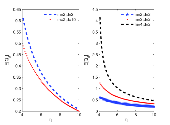
Figure 3: $E[Q_{d}]$ vs $\eta$ for $(m,d)=(2,2),(3,2),(4,2)$ and $(2,10)$

Example two: Performance comparisons between the exponential and PH service times

We consider two related supermarket models with Poisson inputs of arrival rate $N\lambda$: one with exponential service times, and another with PH service times. For the two supermarket models, our goal is to observe the influence of different service time distributions on the performance of this supermarket model. To that end, the parameters of this system are taken as

$$\mu=3.4118,\text{ }\alpha=\left(\frac{1}{2},\frac{1}{2}\right),T=\left(\begin{array}[c]{cc}-5&3\\ 2&-7\end{array}\right).$$

Under the exponential and PH service times, Figure 4 depicts how $E\left[Q_{d}\right]$ and $E\left[T_{d}\right]$ depend on the arrival rate $\lambda\in\left[1,3\right]$ with $\lambda<\mu$, and on the choice number $d=1,2$. It is seen that $E\left[Q_{d}\right]$ and $E\left[T_{d}\right]$ decrease as $d$ increases, while $E\left[Q_{d}\right]$ and $E\left[T_{d}\right]$ increase as $\lambda$ increases.

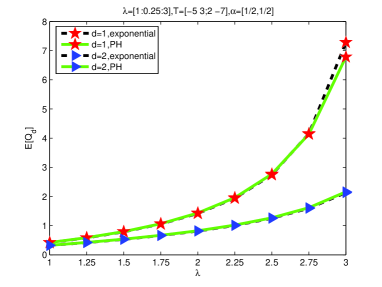
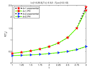
Figure 4: Performance comparison between the exponential and PH service times

Example three: The role of the PH service times

In this supermarket model with $d=2$, the customers arrive at this system as a Poisson process with arrival rate $N\lambda$, and the service times at each server are a PH distribution with irreducible representation $\left(\alpha,T\left(i\right)\right)$, $\alpha=\left(1/2,1/2\right)$,

$$T\left(1\right)=\left(\begin{array}[c]{cc}-5&3\\ 2&-7\end{array}\right),\text{ }T\left(2\right)=\left(\begin{array}[c]{cc}-4&3\\ 2&-7\end{array}\right),\text{ }T\left(3\right)=\left(\begin{array}[c]{cc}-4&4\\ 2&-7\end{array}\right).$$

It is seen that some minor changes are designed in the first rows of the matrices $T\left(i\right)$ for $i=1,2,3$. Let $\lambda=1$. Then

$$\rho\left(1\right)=0.2931,\text{ }\rho\left(2\right)=0.3636,\text{ }\rho\left(3\right)=0.4250.$$

This gives

$$\rho\left(1\right)<\rho\left(2\right)<\rho\left(3\right).$$

Figure 5 indicates how $E\left[T_{d}\right]$ depends on the different transition rate matrices $T\left(i\right)$ for $i=1,2,3$, and

$$E\left[T_{d}\left(1\right)\right]<E\left[T_{d}\left(2\right)\right]<E\left[T_{d}\left(3\right)\right].$$

It is seen that $E\left[T_{d}\right]$ decreases as $d$ increases.

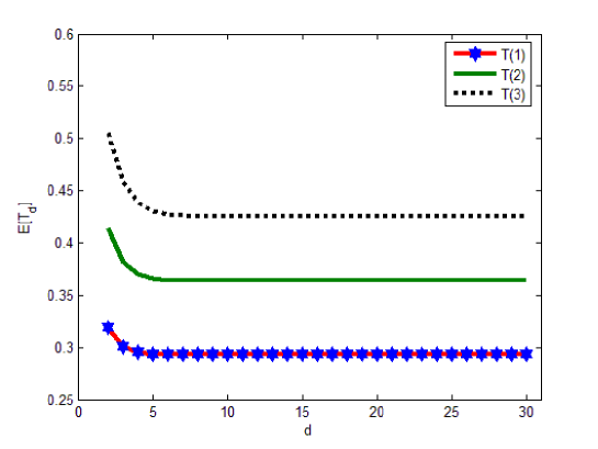
Figure 5: $E\left[T_{d}(i)\right]$ vs the transition rate matrices $T\left(i\right)$ for $i=1,2,3$

Example four: The role of the MAP inputs

In this supermarket model, the service time distribution is exponential with service rate $\mu=1,$ and the arrival processes are the MAP of irreducible matrix descriptor $\left(C\left(N\right),D\left(N\right)\right)$, where

$$C=\left(\begin{array}[c]{cc}-5-\frac{2}{7}\lambda&5\\ 7&-7-2\lambda\end{array}\right),\text{ }D=\left(\begin{array}[c]{cc}\frac{2}{7}\lambda&0\\ 0&2\lambda\end{array}\right).$$

It is easy to check that $\omega=\left(7/12,5/12\right)$, and the stationary arrival rate $\lambda^{\ast}=\omega De=\lambda$. If $\mu=1$ and $\rho=\lambda^{\ast}/\mu=\lambda<1$, then $\lambda\in\left(0,1\right)$.

Figure 6 shows how $E\left[Q_{d}\right]$ and $E\left[T_{d}\right]$ depend on the parameter $\lambda$ of the MAP under different choice numbers $d=1,2,5,10$. It is seen that $E\left[Q_{d}\right]$ and $E\left[T_{d}\right]$ decrease as $d$ increases, while $E\left[Q_{d}\right]$ and $E\left[T_{d}\right]$ increase as $\lambda$ increases.

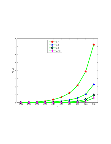
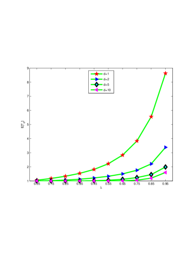
Figure 6: The role of the MAP inputs

8 Concluding Remarks

In this paper, we analyze a more general block-structured supermarket model with non-Poisson MAP inputs and with non-exponential PH service times, and set up an infinite-dimensional system of differential vector equations satisfied by the expected fraction vector through a detailed probability analysis, where an important result: The invariance of environment factors is obtained. We apply the phase-structured operator semigroup to proving the phase-structured mean-field limit, which indicates the asymptotic independence of the block-structured queueing processes in this supermarket model. Furthermore, we provide an effective algorithm for computing the fixed point by means of the matrix-analytic method. Using the fixed point, we provide two performance measures of this supermarket model, and use some numerical examples to illustrate how the two performance measures depend on the non-Poisson MAP inputs and on the non-exponential PH service times. From many practical applications, the block-structured supermarket model is an important queueing model to analyze the relation between the system performance and the job routing rule, and it can also help to design reasonable architecture to improve the performance and to balance the load.

Note that this paper provide a clear picture for how to use the phase-structured mean-field model as well as the matrix-analytic method to analyze performance measures of more general supermarket models. We show that this picture is organized as three key parts: (1) Setting up system of differential equations, (2) necessary proofs of the phase-structured mean-field limit, and (3) performance computation of this supermarket model through the fixed point. Therefore, the results of this paper give new highlight on understanding performance analysis and nonlinear Markov processes for more general supermarket models with non-Poisson inputs and with non-exponential service times. Along such a line, there are a number of interesting directions for potential future research, for example:

• analyzing non-Poisson inputs such as renewal processes;

• studying non-exponential service time distributions, for example, general distributions, matrix-exponential distributions and heavy-tailed distributions; and

• discussing the bulk arrival processes, such as BMAP inputs, and the bulk service processes, where effective algorithms for the fixed point are necessary and interesting.

Up to now, we believe that a larger gap exists when dealing with either renewal inputs or general service times in a supermarket model, because a more challenging infinite-dimensional system of differential equations need be established, a more complicated mean-field limit need be proved, and computation of the fixed point will be more interesting, difficult and challenging.

Three Appendices

Appendix A: Proof of Theorem 1

To prove Equations (14) to (17) in Theorem 1, we need the following computational steps. Note that

$$\sum_{m=1}^{d}C_{d}^{m}\left\{\sum_{j=1}^{m_{B}}\left[u_{k-1;l,j}^{(N)}\left(t\right)-u_{k;l,j}^{(N)}\left(t\right)\right]\right\}^{m-1}\left\{\sum_{j=1}^{m_{B}}\left[u_{k;l,j}^{(N)}\left(t\right)\right]\right\}^{d-m}$$

$$=C_{d}^{d}\left\{\sum_{j=1}^{m_{B}}\left[u_{k-1;l,j}^{(N)}\left(t\right)-u_{k;l,j}^{(N)}\left(t\right)\right]\right\}^{d-1}$$

$$+\sum_{m=1}^{d-1}C_{d}^{m}\left\{\sum_{j=1}^{m_{B}}\left[u_{k-1;l,j}^{(N)}\left(t\right)-u_{k;l,j}^{(N)}\left(t\right)\right]\right\}^{m-1}\left\{\sum_{j=1}^{m_{B}}\left[u_{k;l,j}^{(N)}\left(t\right)\right]\right\}^{d-m}$$

and

$$\sum_{m=1}^{d-1}C_{d}^{m}\left\{\sum_{j=1}^{m_{B}}\left[u_{k-1;l,j}^{(N)}\left(t\right)-u_{k;l,j}^{(N)}\left(t\right)\right]\right\}^{m-1}\left\{\sum_{j=1}^{m_{B}}\left[u_{k;l,j}^{(N)}\left(t\right)\right]\right\}^{d-m}$$

$$+\sum_{m=1}^{d-1}C_{d}^{m}\left\{\sum_{j=1}^{m_{B}}\left[u_{k-1;l,j}^{(N)}\left(t\right)-u_{k;l,j}^{(N)}\left(t\right)\right]\right\}^{m-1}$$

$$\times\sum_{\begin{subarray}{c}r_{1}+r_{2}+\cdots+r_{m_{A}}=d-m\\ \sum_{i\neq l}^{m_{A}}r_{i}\geq 1\\ 0\leq r_{j}\leq d-m,1\leq j\leq m_{A}\end{subarray}}\left(\begin{array}[c]{c}d-m\\ r_{1},r_{2},\ldots,r_{m_{A}}\end{array}\right)\prod_{i=1}^{m_{A}}\left\{\sum_{j=1}^{m_{B}}\left[u_{k;i,j}^{(N)}\left(t\right)\right]\right\}^{r_{i}}$$

$$=\sum_{m=1}^{d-1}C_{d}^{m}\left\{\sum_{j=1}^{m_{B}}\left[u_{k-1;l,j}^{(N)}\left(t\right)-u_{k;l,j}^{(N)}\left(t\right)\right]\right\}^{m-1}\left\{\sum_{i=1}^{m_{A}}\sum_{j=1}^{m_{B}}\left[u_{k;i,j}^{(N)}\left(t\right)\right]\right\}^{d-m},$$

since $\left\{\sum_{j=1}^{m_{B}}\left[u_{k;l,j}^{(N)}\left(t\right)\right]\right\}^{d-m}$ corresponds to the case with $\sum_{i\neq l}^{m_{A}}r_{i}=0$ and $r_{l}=d-m$, and

$$\left\{\sum_{j=1}^{m_{B}}\left[u_{k;l,j}^{(N)}\left(t\right)\right]\right\}^{d-m}+\sum_{\begin{subarray}{c}r_{1}+r_{2}+\cdots+r_{m_{A}}=d-m\\ \sum_{i\neq l}^{m_{A}}r_{i}\geq 1\\ 0\leq r_{j}\leq d-m,1\leq j\leq m_{A}\end{subarray}}\left(\begin{array}[c]{c}d-m\\ r_{1},r_{2},\ldots,r_{m_{A}}\end{array}\right)\prod_{i=1}^{m_{A}}\left\{\sum_{j=1}^{m_{B}}\left[u_{k;i,j}^{(N)}\left(t\right)\right]\right\}^{r_{i}}$$

$$=\sum_{\begin{subarray}{c}r_{1}+r_{2}+\cdots+r_{m_{A}}=d-m\\ 0\leq r_{j}\leq d-m,1\leq j\leq m_{A}\end{subarray}}\left(\begin{array}[c]{c}d-m\\ r_{1},r_{2},\ldots,r_{m_{A}}\end{array}\right)\prod_{i=1}^{m_{A}}\left\{\sum_{j=1}^{m_{B}}\left[u_{k;i,j}^{(N)}\left(t\right)\right]\right\}^{r_{i}}$$

$$=\left\{\sum_{i=1}^{m_{A}}\sum_{j=1}^{m_{B}}\left[u_{k;i,j}^{(N)}\left(t\right)\right]\right\}^{d-m}.$$

we obtain

$$C_{d}^{d}\left\{\sum_{j=1}^{m_{B}}\left[u_{k-1;l,j}^{(N)}\left(t\right)-u_{k;l,j}^{(N)}\left(t\right)\right]\right\}^{d-1}$$

$$+\sum_{m=1}^{d-1}C_{d}^{m}\left\{\sum_{j=1}^{m_{B}}\left[u_{k-1;l,j}^{(N)}\left(t\right)-u_{k;l,j}^{(N)}\left(t\right)\right]\right\}^{m-1}\left\{\sum_{i=1}^{m_{A}}\sum_{j=1}^{m_{B}}u_{k;l,j}^{(N)}\left(t\right)\right\}^{d-m}$$

$$=\sum_{m=1}^{d}C_{d}^{m}\left\{\sum_{j=1}^{m_{B}}\left[u_{k-1;l,j}^{(N)}\left(t\right)-u_{k;l,j}^{(N)}\left(t\right)\right]\right\}^{m-1}\left\{\sum_{i=1}^{m_{A}}\sum_{j=1}^{m_{B}}\left[u_{k;l,j}^{(N)}\left(t\right)\right]\right\}^{d-m}$$

$$=C_{d}^{1}\left\{\sum_{i=1}^{m_{A}}\sum_{j=1}^{m_{B}}\left[u_{k;l,j}^{(N)}\left(t\right)\right]\right\}^{d-1}+\sum_{m=2}^{d}C_{d}^{m}\left\{\sum_{j=1}^{m_{B}}\left[u_{k-1;l,j}^{(N)}\left(t\right)-u_{k;l,j}^{(N)}\left(t\right)\right]\right\}^{m-1}$$

$$\times\left\{\sum_{i=1}^{m_{A}}\sum_{j=1}^{m_{B}}\left[u_{k;l,j}^{(N)}\left(t\right)\right]\right\}^{d-m}.$$

Using $\frac{m_{1}}{m}C_{m}^{m_{1}}=C_{m-1}^{m_{1}-1}$, we can obtain

$$\sum_{m=2}^{d}C_{d}^{m}\left\{\sum_{j=1}^{m_{B}}\left[u_{k-1;l,j}^{(N)}\left(t\right)-u_{k;l,j}^{(N)}\left(t\right)\right]\right\}^{m-1}\left\{\sum_{i=1}^{m_{A}}\sum_{j=1}^{m_{B}}\left[u_{k;l,j}^{(N)}\left(t\right)\right]\right\}^{d-m}$$

$$+\sum_{m=2}^{d}C_{d}^{m}\sum_{m_{1}=1}^{m-1}\frac{m_{1}}{m}C_{m}^{m_{1}}\left\{\sum_{j=1}^{m_{B}}\left[u_{k-1;l,j}^{(N)}\left(t\right)-u_{k;l,j}^{(N)}\left(t\right)\right]\right\}^{m_{1}-1}$$

$$\times\sum_{\begin{subarray}{c}n_{1}+n_{2}+\cdots+n_{m_{A}}=m-m_{1}\\ \sum_{i\neq l}^{m_{A}}n_{i}\geq 1\\ 0\leq n_{j}\leq m-m_{1},1\leq j\leq m_{A}\end{subarray}}\left(\begin{array}[c]{c}m-m_{1}\\ n_{1},n_{2},\ldots,n_{m_{A}}\end{array}\right)$$

$$\times\prod_{i=1}^{m_{A}}\left\{\sum_{j=1}^{m_{B}}\left[u_{k-1;i,j}^{(N)}\left(t\right)-u_{k;i,j}^{(N)}\left(t\right)\right]\right\}^{n_{i}}$$

$$\times\sum_{\begin{subarray}{c}r_{1}+r_{2}+\cdots+r_{m_{A}}=d-m\\ 0\leq r_{j}\leq d-m,1\leq j\leq m_{A}\end{subarray}}\left(\begin{array}[c]{c}d-m\\ r_{1},r_{2},\ldots,r_{m_{A}}\end{array}\right)\prod_{i=1}^{m_{A}}\left\{\sum_{j=1}^{m_{B}}u_{k;i,j}^{(N)}\left(t\right)\right\}^{r_{i}}$$

$$=\sum_{m=2}^{d}C_{d}^{m}\sum_{m_{1}=1}^{m}C_{m-1}^{m_{1}-1}\left\{\sum_{j=1}^{m_{B}}\left[u_{k-1;l,j}^{(N)}\left(t\right)-u_{k;l,j}^{(N)}\left(t\right)\right]\right\}^{m_{1}-1}$$

$$\times\sum_{\begin{subarray}{c}n_{1}+n_{2}+\cdots+n_{m_{A}}=m-m_{1}\\ 0\leq n_{j}\leq m-m_{1},1\leq j\leq m_{A}\end{subarray}}\left(\begin{array}[c]{c}m-m_{1}\\ n_{1},n_{2},\ldots,n_{m_{A}}\end{array}\right)$$

$$\times\prod_{i=1}^{m_{A}}\left\{\sum_{j=1}^{m_{B}}\left[u_{k-1;i,j}^{(N)}\left(t\right)-u_{k;i,j}^{(N)}\left(t\right)\right]\right\}^{n_{i}}\left\{\sum_{i=1}^{m_{A}}\sum_{j=1}^{m_{B}}\left[u_{k;l,j}^{(N)}\left(t\right)\right]\right\}^{d-m}$$

$$=\sum_{m=2}^{d}C_{d}^{m}\sum_{m_{1}=1}^{m}\frac{m_{1}}{m}C_{m}^{m_{1}}\left\{\sum_{j=1}^{m_{B}}\left[u_{k-1;l,j}^{(N)}\left(t\right)-u_{k;l,j}^{(N)}\left(t\right)\right]\right\}^{m_{1}-1}$$

$$\times\left\{\sum_{i\neq l}^{m_{A}}\sum_{j=1}^{m_{B}}\left[u_{k-1;i,j}^{(N)}\left(t\right)-u_{k;i,j}^{(N)}\left(t\right)\right]\right\}^{m-m_{1}}\left\{\sum_{i=1}^{m_{A}}\sum_{j=1}^{m_{B}}\left[u_{k;i,j}^{(N)}\left(t\right)\right]\right\}^{d-m}$$

$$=\sum_{m=2}^{d}C_{d}^{m}\sum_{m_{1}-1=0}^{m-1}C_{m-1}^{m_{1}-1}\left\{\sum_{j=1}^{m_{B}}\left[u_{k-1;l,j}^{(N)}\left(t\right)-u_{k;l,j}^{(N)}\left(t\right)\right]\right\}^{m_{1}-1}$$

$$\times\left\{\sum_{i\neq l}^{m_{A}}\sum_{j=1}^{m_{B}}\left[u_{k-1;i,j}^{(N)}\left(t\right)-u_{k;i,j}^{(N)}\left(t\right)\right]\right\}^{m-1-\left(m_{1}-1\right)}\left\{\sum_{i=1}^{m_{A}}\sum_{j=1}^{m_{B}}\left[u_{k;i,j}^{(N)}\left(t\right)\right]\right\}^{d-m}$$

$$=\sum_{m=2}^{d}C_{d}^{m}\left\{\sum_{i=1}^{m_{A}}\sum_{j=1}^{m_{B}}\left[u_{k-1;i,j}^{(N)}\left(t\right)-u_{k;i,j}^{(N)}\left(t\right)\right]\right\}^{m-1}\left\{\sum_{i=1}^{m_{A}}\sum_{j=1}^{m_{B}}\left[u_{k;i,j}^{(N)}\left(t\right)\right]\right\}^{d-m},$$

we have

$$C_{d}^{1}\left\{\sum_{i=1}^{m_{A}}\sum_{j=1}^{m_{B}}\left[u_{k;l,j}^{(N)}\left(t\right)\right]\right\}^{d-1}$$

$$+\sum_{m=2}^{d}C_{d}^{m}\left\{\sum_{i=1}^{m_{A}}\sum_{j=1}^{m_{B}}\left[u_{k-1;i,j}^{(N)}\left(t\right)-u_{k;i,j}^{(N)}\left(t\right)\right]\right\}^{m-1}\left\{\sum_{i=1}^{m_{A}}\sum_{j=1}^{m_{B}}\left[u_{k;i,j}^{(N)}\left(t\right)\right]\right\}^{d-m}$$

$$=\sum_{m=1}^{d}C_{d}^{m}\left\{\sum_{i=1}^{m_{A}}\sum_{j=1}^{m_{B}}\left[u_{k-1;i,j}^{(N)}\left(t\right)-u_{k;i,j}^{(N)}\left(t\right)\right]\right\}^{m-1}\left\{\sum_{i=1}^{m_{A}}\sum_{j=1}^{m_{B}}\left[u_{k;i,j}^{(N)}\left(t\right)\right]\right\}^{d-m}.$$

Thus for $k\geq 1$ we obtain

$$L_{k;l}^{\left(N\right)}\left(u_{k-1}^{\left(N\right)}\left(t\right),u_{k}^{\left(N\right)}\left(t\right)\right)= \sum_{m=1}^{d}C_{d}^{m}\left\{\sum_{i=1}^{m_{A}}\sum_{j=1}^{m_{B}}\left[u_{k-1;i,j}^{(N)}\left(t\right)-u_{k;i,j}^{(N)}\left(t\right)\right]\right\}^{m-1}$$

$$\times\left\{\sum_{i=1}^{m_{A}}\sum_{j=1}^{m_{B}}\left[u_{k;i,j}^{(N)}\left(t\right)\right]\right\}^{d-m},$$

which is independent of phase $l\in\left\{1,2,\ldots,m_{A}\right\}$. Thus we have

$$L_{k}^{\left(N\right)}\left(u_{k-1}^{\left(N\right)}\left(t\right),u_{k}^{\left(N\right)}\left(t\right)\right)=L_{k;l}^{\left(N\right)}\left(u_{k-1}^{\left(N\right)}\left(t\right),u_{k}^{\left(N\right)}\left(t\right)\right).$$

Similarly, for phase $l\in\left\{1,2,\ldots,m_{A}\right\}$, we have

$$L_{1;l}^{\left(N\right)}\left(\left[u_{0}^{\left(N\right)}\left(t\right)\otimes\alpha\right],u_{1}^{\left(N\right)}\left(t\right)\right)= \sum_{m=1}^{d}C_{d}^{m}\left[\sum_{i=1}^{m_{A}}\sum_{j=1}^{m_{B}}\left(u_{0;i}^{\left(N\right)}\left(t\right)\alpha_{j}-u_{1;i,j}^{\left(N\right)}\left(t\right)\right)\right]^{m-1}$$

$$\times\left[\sum_{i=1}^{m_{A}}\sum_{j=1}^{m_{B}}u_{1;i,j}^{\left(N\right)}\left(t\right)\right]^{d-m}.$$

This gives

$$L_{1}^{\left(N\right)}\left(\left[u_{0}^{\left(N\right)}\left(t\right)\otimes\alpha\right],u_{1}^{\left(N\right)}\left(t\right)\right)=L_{1;l}^{\left(N\right)}\left(\left[u_{0}^{\left(N\right)}\left(t\right)\otimes\alpha\right],u_{1}^{\left(N\right)}\left(t\right)\right)$$

This completes the proof.  

Appendix B: The Mean-Field Limit

In this appendix, we use the operator semigroup to provide a mean-field limit for the sequence of Markov processes $\{\mathbf{U}^{(N)}(t),t\geq 0\}$, which indicates the asymptotic independence of the block-structured queueing processes in this supermarket model. Note that the limits of the sequences of Markov processes can usually be discussed by the three main techniques: Operator semigroups, martingales, and stochastic equations. Readers may refer to Ethier and Kurtz [4] for more details.

To use the operator semigroups of Markov processes, we first need to introduce some state spaces as follows. For the vectors $\mathbf{u}^{\left(N\right)}=\left(u_{0}^{\left(N\right)},u_{1}^{\left(N\right)},u_{2}^{{}^{(N)}}\left(t\right)\ldots\right)$ where $u_{0}^{\left(N\right)}$ is a probability vector of size $m_{A}$ and the size of the row vector $u_{k}^{\left(N\right)}$ is $m_{A}m_{B}$ for $k\geq 1$, we write

$$\widetilde{\Omega}_{N}= \left\{\mathbf{u}^{\left(N\right)}:u_{1}^{\left(N\right)}\geq u_{2}^{\left(N\right)}\geq u_{3}^{\left(N\right)}\geq\cdots\geq 0,\right.$$

$$\left.1=u_{0}^{\left(N\right)}e\geq u_{1}^{\left(N\right)}e\geq u_{2}^{\left(N\right)}e\geq\cdots\geq 0,\right.$$

$$\left.Nu_{k}^{\left(N\right)}\text{ \ is a vector of nonnegative integers for }k\geq 0\right\}.$$

and

$$\Omega_{N}=\left\{\mathbf{u}^{\left(N\right)}\in\widetilde{\Omega}_{N}:\mathbf{u}^{\left(N\right)}e<+\infty\right\}.$$

At the same time, for the vector $\mathbf{u}=\left(u_{0},u_{1},u_{2},\ldots\right)$ where $u_{0}$ is a probability vector of size $m_{A}$ and the size of the row vector $u_{k}$ is $m_{A}m_{B}$ for $k\geq 1$, we set

$$\widetilde{\Omega}=\{\mathbf{u}:u_{1}\geq u_{2}\geq u_{3}\geq\cdots\geq 0;\ \ 1=u_{0}^{\left(N\right)}e\geq u_{1}^{\left(N\right)}e\geq u_{2}^{\left(N\right)}e\geq\cdots\geq 0\}$$

and

$$\Omega=\left\{\mathbf{u}\in\widetilde{\Omega}:\mathbf{u}e<+\infty\right\}.$$

Obviously, $\Omega_{N}\subsetneqq\Omega\subsetneqq\widetilde{\Omega}$ and $\Omega_{N}\subsetneqq\widetilde{\Omega}_{N}\subsetneqq\widetilde{\Omega}$.

In the vector space $\widetilde{\Omega}$, we take a metric

$$\rho\left(\mathbf{u},\mathbf{u}^{\prime}\right) =\max\left\{\max_{1\leq i\leq m_{A}}\left\{|u_{0;i}-u_{0;i}^{\prime}|\right\},\right.$$

$$\left.\max_{\begin{subarray}{c}0\leq i\leq m_{A}\\ 0\leq j\leq m_{B}\end{subarray}}\sup_{k\geq 1}\left\{\dfrac{|u_{k;i,j}-u_{k;i,j}^{\prime}|}{k+1}\right\}\right\}$$ (72)

for $\mathbf{u},\mathbf{u}^{\prime}\in\widetilde{\Omega}$. Note that under the metric $\rho\left(\mathbf{u},\mathbf{u}^{\prime}\right),$ the vector space $\widetilde{\Omega}$ is separable and compact.

B.1: The operator semigroup

For $\mathbf{g}\in\Omega_{N}$, we write

$$L_{1}\left(g_{0}\otimes\alpha,g_{1}\right)=\sum_{m=1}^{d}C_{d}^{m}\left[\sum_{l=1}^{m_{A}}\sum_{j=1}^{m_{B}}\left(g_{0;l}\left(t\right)\alpha_{j}-g_{1;l,j}\right)\right]^{m-1}\left(\sum_{l=1}^{m_{A}}\sum_{j=1}^{m_{B}}g_{1;l,j}\right)^{d-m},$$

and for $k\geq 2$

$$L_{k}\left(g_{k-1},g_{k}\right)=\sum_{m=1}^{d}C_{d}^{m}\left[\sum_{l=1}^{m_{A}}\sum_{j=1}^{m_{B}}\left(g_{k-1;l,j}-g_{k;l,j}\right)\right]^{m-1}\left[\sum_{l=1}^{m_{A}}\sum_{j=1}^{m_{B}}g_{k;l,j}\right]^{d-m}.$$

Now, we consider the infinite-dimensional Markov process $\{\mathbf{U}^{(N)}(t),t\geq 0\}$ on state space $\Omega_{N}$ (or $\widetilde{\Omega}_{N}$ in a similar analysis) for $N=1,2,3,\ldots$. Note that the stochastic evolution of this supermarket model of $N$ identical servers is described as the Markov process $\left\{\mathbf{U}^{(N)}(t),t\geq 0\right\}$, where

$$\frac{\text{d}}{\text{d}t}\left(\mathbf{U}^{(N)}(t)\right)=\mathbf{A}_{N}\text{ }f\left(\mathbf{U}^{(N)}(t)\right),$$

where $\mathbf{A}_{N}$ acting on functions $f:\Omega_{N}\rightarrow\mathbf{C}^{1}$ is the generating operator of the Markov process $\left\{\mathbf{U}^{(N)}(t),t\geq 0\right\}$,

$$\mathbf{A}_{N}=\mathbf{A}_{N}^{\text{A-In}}+\mathbf{A}_{N}^{\text{A-Transition}}+\mathbf{A}_{N}^{\text{S-Transition}}+\mathbf{A}_{N}^{\text{S-Out}},$$ (73)

for $\mathbf{g}\in\Omega_{N}$

$$\mathbf{A}_{N}^{\text{A-In}}f(\mathbf{g})= N\sum\limits_{k=2}^{\infty}\sum_{j=1}^{m_{B}}\sum_{i=1}^{m_{A}}\left[\sum_{l=1}^{m_{A}}\left(g_{k-1;l,j}d_{l,i}-g_{k;i,j}\sum_{q=1}^{m_{A}}d_{i,q}\right)L_{k}\left(g_{k-1},g_{k}\right)\right]$$

$$\times\left[f\left(\mathbf{g}+\frac{e_{k;i,j}}{N}\right)-f\left(\mathbf{g}\right)\right]$$

$$+N\sum_{j=1}^{m_{B}}\sum_{i=1}^{m_{A}}\left[\sum_{l=1}^{m_{A}}\left(g_{0;l}d_{l,i}\alpha_{j}-g_{1;i,j}\sum_{q=1}^{m_{A}}d_{i,q}\right)L_{1}\left(g_{0}\otimes\alpha,g_{1}\right)\right]$$

$$\times\left[f\left(\mathbf{g}+\frac{e_{1;i,j}}{N}\right)-f\left(\mathbf{g}\right)\right],$$ (74)

$$\mathbf{A}_{N}^{\text{A-Transition}}= N\sum\limits_{k=1}^{\infty}\sum_{j=1}^{m_{B}}\sum_{i=1}^{m_{A}}\sum_{l=1}^{m_{A}}\left[g_{k;l,j}c_{l,i}+g_{k;i,j}\sum_{q=1}^{m_{A}}d_{i,q}\right]$$

$$\times\left[f\left(\mathbf{g}-\frac{e_{k;l,j}}{N}+\frac{e_{k;i,j}}{N}\right)-f\left(\mathbf{g}\right)\right]$$

$$+N\sum_{i=1}^{m_{A}}\sum_{l=1}^{m_{A}}\left[g_{0;l}c_{l,i}+g_{0,i}\sum_{q=1}^{m_{A}}d_{i,q}\right]$$

$$\times\left[f\left(\mathbf{g}-\frac{e_{0;l}}{N}+\frac{e_{0;i}}{N}\right)-f\left(\mathbf{g}\right)\right],$$ (75)

$$\mathbf{A}_{N}^{\text{S-Transition}} =N\sum\limits_{k=1}^{\infty}\sum_{i=1}^{m_{A}}\sum_{j=1}^{m_{B}}\sum_{r=1}^{m_{B}}\left(g_{k;i,r}t_{r,j}\right)$$

$$\times\left[f(\mathbf{g}-\dfrac{\mathbf{e}_{k;i,r}}{N}+\dfrac{\mathbf{e}_{k;i,j}}{N})-f(\mathbf{g})\right]$$ (76)

and

$$\mathbf{A}_{N}^{\text{S-Out}}=N\sum\limits_{k=1}^{\infty}\sum_{i=1}^{m_{A}}\sum_{j=1}^{m_{B}}\sum_{r=1}^{m_{B}}\left(g_{k+1;i,r}t_{r}^{0}\alpha_{j}\right)\left[f(\mathbf{g})-f(\mathbf{g-}\frac{\mathbf{e}_{k;i,j}}{N})\right],$$ (77)

where $\mathbf{e}_{k;l,j}$ is a row vector of infinite size with the $\left(k;i,j\right)$th entry being one and all others being zero. Thus it follows from Equations (73) to (77) that

$$\mathbf{A}_{N}f(\mathbf{g})= N\sum\limits_{k=2}^{\infty}\sum_{j=1}^{m_{B}}\sum_{i=1}^{m_{A}}\left[\sum_{l=1}^{m_{A}}\left(g_{k-1;l,j}d_{l,i}-g_{k;i,j}\sum_{q=1}^{m_{A}}d_{i,q}\right)L_{k}\left(g_{k-1},g_{k}\right)\right]$$

$$\times\left[f\left(\mathbf{g}+\frac{e_{k;i,j}}{N}\right)-f\left(\mathbf{g}\right)\right]$$

$$+N\sum_{j=1}^{m_{B}}\sum_{i=1}^{m_{A}}\left[\sum_{l=1}^{m_{A}}\left(g_{0;l}d_{l,i}\alpha_{j}-g_{1;i,j}\sum_{q=1}^{m_{A}}d_{i,q}\right)L_{1}\left(g_{1}\otimes\alpha,g_{1}\right)\right]$$

$$\times\left[f\left(\mathbf{g}+\frac{e_{1;i,j}}{N}\right)-f\left(\mathbf{g}\right)\right]$$

$$+N\sum\limits_{k=1}^{\infty}\sum_{j=1}^{m_{B}}\sum_{i=1}^{m_{A}}\sum_{l=1}^{m_{A}}\left(g_{k;l,j}c_{l,i}+g_{k;i,j}\sum_{q=1}^{m_{A}}d_{i,q}\right)$$

$$\times\left[f\left(\mathbf{g}-\frac{e_{k;l,j}}{N}+\frac{e_{k;i,j}}{N}\right)-f\left(\mathbf{g}\right)\right]$$

$$+N\sum_{i=1}^{m_{A}}\sum_{l=1}^{m_{A}}\left(g_{0;l}c_{l,i}+\sum_{q=1}^{m_{A}}d_{i,q}\right)\left[f\left(\mathbf{g}-\frac{e_{0;l}}{N}+\frac{e_{0;i}}{N}\right)-f\left(\mathbf{g}\right)\right]$$

$$+N\sum\limits_{k=1}^{\infty}\sum_{i=1}^{m_{A}}\sum_{j=1}^{m_{B}}\sum_{r=1}^{m_{B}}\left\{\left(g_{k;i,r}t_{r,j}\right)\left[f(\mathbf{g}-\dfrac{\mathbf{e}_{k;i,r}}{N}+\dfrac{\mathbf{e}_{k;i,j}}{N})-f(\mathbf{g})\right]\right.$$

$$\left.+\left(g_{k+1;i,r}t_{r}^{0}\alpha_{j}\right)\left[f(\mathbf{g})-f(\mathbf{g}-\frac{\mathbf{e}_{k;i,j}}{N})\right]\right\}.$$ (78)

Remark 5

If the MAP is a Poisson process, then $m_{A}=1$ and $C=-\lambda$ and $D=\lambda$; and if the PH service time distribution is exponential, then $m_{B}=1$, $T=-\mu$ and $T^{0}\alpha=\mu$. In this case, it is easy to check from (78) that

$$\mathbf{A}_{N}f(\mathbf{g})= \lambda N\left(1-g_{1}^{d}\right)\left[f\left(\mathbf{g}+\frac{e_{1}}{N}\right)-f\left(\mathbf{g}\right)\right]$$

$$+\lambda N\sum\limits_{k=2}^{\infty}\left(g_{k-1}^{d}-g_{k}^{d}\right)\left[f\left(\mathbf{g}+\frac{e_{k}}{N}\right)-f\left(\mathbf{g}\right)\right]$$

$$-\mu N\sum\limits_{n=1}^{\infty}\left(g_{n}-g_{n+1}\right)\left[f\left(\mathbf{g}\right)-f\left(\mathbf{g}-\frac{e_{n}}{N}\right)\right],$$

which is the same as (1.5) for $d=2$ in Vvedenskaya et al [32].

B.2: The mean-Field limit

We compute

$$\lim_{N\rightarrow\infty}\frac{f\left(\mathbf{g}+\dfrac{e_{k;i,j}}{N}\right)-f\left(\mathbf{g}\right)}{\dfrac{1}{N}}=\frac{\partial}{\partial g_{k;i,j}}f(\mathbf{g}),$$

$$\lim_{N\rightarrow\infty}\frac{f\left(\mathbf{g}\right)-f\left(\mathbf{g-}\dfrac{e_{k;i,j}}{N}\right)}{\dfrac{1}{N}}=\frac{\partial}{\partial g_{k;i,j}}f(\mathbf{g})$$

and

$$\lim_{N\rightarrow\infty}\frac{f\left(\mathbf{g-}\dfrac{e_{k;l,j}}{N}+\dfrac{e_{k;i,j}}{N}\right)-f\left(\mathbf{g}\right)}{\dfrac{1}{N}}=\frac{\partial}{\partial g_{k;i,j}}f(\mathbf{g})-\frac{\partial}{\partial g_{k;l,j}}f(\mathbf{g}).$$

The operator semigroup of the Markov process $\left\{\mathbf{U}^{(N)}(t),t\geq 0\right\}$ is defined as $\mathbf{T}_{N}(t)$, where if $f:\Omega_{N}\rightarrow\mathbf{C}^{1}$, then for $\mathbf{g}\in\Omega_{N}$ and $t\geq 0$

$$\mathbf{T}_{N}(t)f(\mathbf{g})=E\left[f(\mathbf{U}_{N}(t)\text{ }|\text{ }\mathbf{U}_{N}(0)=\mathbf{g}\right].$$ (79)

Note that $\mathbf{A}_{N}$ is the generating operator of the operator semigroup $\mathbf{T}_{N}(t)$, it is easy to see that $\mathbf{T}_{N}(t)=\exp\left\{\mathbf{A}_{N}t\right\}$ for $t\geq 0$.

Definition 1

A operator semigroup $\left\{\mathbf{S}\left(t\right):t\geq 0\right\}$ on the Banach space $L=C(\widetilde{\Omega})$ is said to be strongly continuous if $\lim_{t\rightarrow 0}\mathbf{S}\left(t\right)f=f$ for every $f\in L$; it is said to be a contractive semigroup if $\left\|\mathbf{S}\left(t\right)\right\|\leq 1$ for $t\geq 0$.

Let $L=C(\widetilde{\Omega})$ be the Banach space of continuous functions $f:\widetilde{\Omega}\rightarrow\mathbf{R}$ with uniform metric $\left\|f\right\|=\underset{u\in\widetilde{\Omega}}{\max}\left|f(u)\right|$, and similarly, let $L_{N}=C(\Omega_{N})$. The inclusion $\Omega_{N}\subset\widetilde{\Omega}$ induces a contraction mapping $\Pi_{N}:L\rightarrow L_{N},\Pi_{N}f(u)=f(u)$ for $f\in L$ and $u\in\Omega_{N}$.

Now, we consider the limiting behavior of the sequence $\{(\mathbf{U}^{(N)}(t),t\geq 0\}$ of Markov processes for $N=1,2,3,\ldots$. Two formal limits for the sequence $\left\{\mathbf{A}_{N}\right\}$ of generating operators and for the sequence $\left\{\mathbf{T}_{N}(t)\right\}$ of semigroups are expressed as $\mathbf{A}=\lim_{N\rightarrow\infty}\mathbf{A}_{N}$ and $\mathbf{T}\left(t\right)=\lim_{N\rightarrow\infty}\mathbf{T}_{N}(t)$ for $t\geq 0$, respectively. It follows from (78) that as $N\rightarrow\infty$

$$\mathbf{A}f(\mathbf{g})= \sum\limits_{k=2}^{\infty}\sum_{j=1}^{m_{B}}\sum_{i=1}^{m_{A}}\left[\sum_{l=1}^{m_{A}}\left(g_{k-1;l,j}d_{l,i}-g_{k;i,j}\sum_{q=1}^{m_{A}}d_{i,q}\right)L_{k}\left(g_{k-1},g_{k}\right)\right]\frac{\partial}{\partial g_{k;i,j}}f(\mathbf{g})$$

$$+\sum_{j=1}^{m_{B}}\sum_{i=1}^{m_{A}}\left[\sum_{l=1}^{m_{A}}\left(g_{0;l}d_{l,i}\alpha_{j}-g_{1;i,j}\sum_{q=1}^{m_{A}}d_{i,q}\right)L_{1}\left(g_{0}\otimes\alpha,g_{1}\right)\right]\frac{\partial}{\partial g_{1;i,j}}f(\mathbf{g})$$

$$+\sum\limits_{k=1}^{\infty}\sum_{j=1}^{m_{B}}\sum_{i=1}^{m_{A}}\sum_{l=1}^{m_{A}}\left(g_{k;l,j}c_{l,i}+g_{k;i,j}\sum_{q=1}^{m_{A}}d_{i,q}\right)\left[\frac{\partial}{\partial g_{k;i,j}}f(\mathbf{g})-\frac{\partial}{\partial g_{k;l,j}}f(\mathbf{g})\right]$$

$$+\sum_{i=1}^{m_{A}}\sum_{l=1}^{m_{A}}\left(g_{0;l}c_{l,i}+g_{0,i}\sum_{q=1}^{m_{A}}d_{i,q}\right)\left[\frac{\partial}{\partial g_{0;i}}f(\mathbf{g})-\frac{\partial}{\partial g_{0;l}}f(\mathbf{g})\right]$$

$$+\sum\limits_{k=1}^{\infty}\sum_{i=1}^{m_{A}}\sum_{j=1}^{m_{B}}\sum_{r=1}^{m_{B}}\left\{\left(g_{k;i,r}t_{r,j}\right)\left[\frac{\partial}{\partial g_{k;i,j}}f(\mathbf{g})-\frac{\partial}{\partial g_{k;r,r}}f(\mathbf{g})\right]\right.$$

$$+\left.\left(g_{k+1;i,r}t_{r}^{0}\alpha_{j}\right)\frac{\partial}{\partial g_{k;i,j}}f(\mathbf{g})\right\}.$$ (80)

We define a mapping: $\mathbf{g}\rightarrow\mathbf{u}(t,\mathbf{g})$, where $\mathbf{u}(t,\mathbf{g)}$ is a solution to the system of differential vector equations (27) to (31). Note that the operator semigroup $\mathbf{T}(t)$ acts in the space $L$, thus if $f\in L$ and $\mathbf{g}\in\widetilde{\Omega}$, then

$$\mathbf{T}(t)f(\mathbf{g})=f\left(\mathbf{u}(t,\mathbf{g})\right).$$ (81)

From (78) and (80), it is easy to see that the operator semigroups $\mathbf{T}_{N}(t)$ and $\mathbf{T}(t)$ are strongly continuous and contractive, see, for example, Section 1.1 in Chapter one of Ethier and Kurtz [4]. We denote by $\mathcal{D}(\mathbf{A})$ the domain of the generating operator $\mathbf{A}$. It follows from (81) that if $f$ is a function from $L$ and has the partial derivatives $\dfrac{\partial}{\partial g_{k;i,j}}f\left(\mathbf{g}\right)$ $\in L$ for $k\geq 1,1\leq i\leq m_{A},1\leq j\leq m_{B}$, and $\sup_{k\geq 1,1\leq i\leq m_{A},1\leq j\leq m_{B}}\left\{\left|\dfrac{\partial}{\partial g_{k;i,j}}f(\mathbf{g})\right|\right\}<\infty$, then $f\in\mathcal{D}(\mathbf{A})$.

Let $\mathbf{D}$ be the set of all functions $f\in L$ that have the partial derivatives $\dfrac{\partial}{\partial g_{k;i,j}}f\left(\mathbf{g}\right)$ and $\dfrac{\partial^{2}}{\partial g_{k_{1};m,n}\partial g_{k_{2};r;s}}f(\mathbf{g})$, and there exists $C=C(f)<+\infty$ such that

$$\sup_{\begin{subarray}{c}k\geq 1\\ 1\leq i\leq m_{A},1\leq j\leq m_{B}\\ \mathbf{g}\in\widetilde{\Omega}\end{subarray}}\left\{\left|\dfrac{\partial}{\partial g_{k;i,j}}f(\mathbf{g})\right|\right\}<C$$ (82)

and

$$\sup_{\begin{subarray}{c}{}_{\begin{subarray}{c}k_{1},k_{2}\geq 1\\ 1\leq m,r\leq m_{A},1\leq n,s\leq m_{B}\end{subarray}}\\ \mathbf{g}\in\widetilde{\Omega}\end{subarray}}\left\{\left|\dfrac{\partial^{2}}{\partial g_{k_{1};m,n}\partial g_{k_{2};r;s}}f(\mathbf{g})\right|\right\}<C.$$ (83)

We call that $f\in L$ depends only on the first $K$ subvectors if for $\mathbf{g}^{\left(1\right)}$, $\mathbf{g}^{\left(2\right)}\in\widetilde{\Omega},$ it follows from $g_{i}^{\left(1\right)}=g_{i}^{\left(2\right)}$ for $1\leq i\leq K$ that $f(\mathbf{g}^{\left(1\right)})=f(\mathbf{g}^{\left(2\right)})$, where $g_{i}^{\left(1\right)}$ and $g_{i}^{\left(2\right)}$ are row vectors of size $m_{A}m_{B}$ for $1\leq i\leq K$. A similar and simple proof of that in Proposition 2 in Vvedenskaya et al [32] can show that the set of functions from $L$ that depends on the first finite subvectors is dense in $L$.

The following lemma comes from Proposition 1 in Vvedenskaya et al [32]. We restated it here for convenience of description.

Lemma 1

Consider an infinite-dimensional system of differential equations: For $k\geq 0,$

$$z_{k}\left(0\right)=c_{k}$$

and

$$\dfrac{\text{d}z_{k}(t)}{\text{d}t}=\sum\limits_{i=0}^{\infty}z_{i}(t)a_{i,k}(t)+b_{k}(t),$$

and let $\sum\limits_{i=0}^{\infty}\left|a_{i,k}(t)\right|\leq a,\left|b_{k}(t)\right|\leq b_{0}\exp\left\{bt\right\},\left|c_{k}\right|\leq\varrho,b_{0}\geq 0$ and $a<b$. Then

$$z_{k}(t)\leq\varrho\exp\left\{at\right\}+\dfrac{b_{0}}{b-a}\left[\exp\left\{bt\right\}-\exp\left\{at\right\}\right].$$

Definition 2

Let $A$ be a closed linear operator on the Banach space $L=C(\widetilde{\Omega})$. A subspace $\mathbf{D}$ of $\mathcal{D}\left(A\right)$ is said to be a core for $A$ if the closure of the restriction of $A$ to $\mathbf{D}$ is equal to $A$, i.e., $\overline{A|_{\mathbf{D}}}=A$.

For any matrix $\mathbf{A}=\left(a_{i,j}\right)$, we define its norm as follows:

$$\left\|\mathbf{A}\right\|=\max_{i}\left\{\sum\limits_{j}\left|a_{i,j}\right|\right\}.$$

It is easy to compute that

$$\left\|I\otimes\mathbf{A}\right\|=\left\|\mathbf{A}\right\|,$$

$$\left\|\mathbf{A}\otimes I\right\|=\left\|\mathbf{A}\right\|,$$

$$\left\|\text{diag}\left(De\right)\right\|=\left\|D\right\|.$$

We introduce some notation

$$M_{1}=\sum_{m=1}^{d}C_{d}^{m}=2^{d}-1,$$

$$M_{2}=m_{A}m_{B}\sum_{m=1}^{d}C_{d}^{m}\left(d+m-2\right),$$

$$a=\left\|T^{0}\alpha\right\|+\left\|\left[C+\text{diag}\left(De\right)\right]\oplus T\right\|+2\left\|D\right\|\left(M_{1}+M_{2}\right).$$

The following lemma is a key to prove that the set$\mathcal{\ }\mathbf{D}$ is a core for the generating operator $\mathbf{A}$.

Lemma 2

Let $\mathbf{u}(t)$ be a solution to the system of differential vector equations (27) to (28). Then

$$\underset{1\leq i,m\leq m_{A},1\leq j,n\leq m_{B}}{\underset{k,k_{1}\geq 1}{\sup}}\left\{\left|\dfrac{\partial u_{k;i,j}(t,\mathbf{g})}{\partial g_{k_{1};m,n}}\right|\right\}\leq\varrho\exp\left\{at\right\},$$ (84)

and

$$\sup_{\begin{subarray}{c}k,k_{1},k_{2}\geq 1\\ 1\leq i,m,r\leq m_{A}\\ 1\leq j,n,s\leq m_{B}\end{subarray}}\left\{\left|\dfrac{\partial^{2}u_{k;i,j}(t,\mathbf{g})}{\partial g_{k_{1};m,n}\partial g_{k_{2};r;s}}\right|\right\}\leq\widehat{\varrho}\exp\left\{at\right\}+\frac{2\left\|D\right\|}{a}\left(\exp\left\{2at\right\}-\exp\left\{at\right\}\right).$$ (85)

Proof: We only prove Inequalities (84), while Inequalities (85) can be proved similarly.

Notice that $\mathbf{u}(t)$ is a solution to the system of differential vector equations (27) to (28) and possesses the derivatives $\dfrac{\partial u_{k;i,j}(t,\mathbf{g})}{\partial g_{k_{1};m,n}}$ and $\dfrac{\partial^{2}u_{k;i,j}(t,\mathbf{g})}{\partial g_{k_{1};m,n}\partial g_{k_{2};r;s}}$. For simplicity of description, we set $u_{k;i,j,k_{1};m,n}^{\prime}=\dfrac{\partial u_{k;i,j}(t,\mathbf{g})}{\partial g_{k_{1};m,n}}$. It follows from (27) to (28) that for $k,k_{1}\geq$ $1$, $1\leq i,m\leq m_{A}$ and $1\leq j,n\leq m_{B}$,

$$\dfrac{\text{d}u_{k;i,j,k_{1};m,n}^{\prime}}{\text{d}t}= \sum\limits_{l=1}^{m_{A}}\left(u_{k-1;l,j,k_{1};m,n}^{\prime}d_{l,i}-u_{k;i,j,k_{1};m,n}^{\prime}\sum\limits_{q=1}^{m_{A}}d_{i,q}\right)L_{k}\left(u_{k-1}\left(t\right),u_{k}\left(t\right)\right)$$

$$+\sum\limits_{l=1}^{m_{A}}\left(u_{k-1;l,j}d_{l,i}-u_{k;l,j}\sum\limits_{q=1}^{m_{A}}d_{i,q}\right)L_{k}^{\prime}\left(u_{k-1}\left(t\right),u_{k}\left(t\right)\right)$$

$$+\sum\limits_{l=1}^{m_{A}}u_{k;l,j,k_{1};m,n}^{\prime}c_{l,i}+u_{k;i,j,k_{1};m,n}^{\prime}\sum_{q=1}^{m_{A}}d_{i,q}$$

$$+\sum_{s=1}^{m_{B}}u_{k;i,s,k_{1};m,n}^{\prime}t_{s,j}+\sum_{s=1}^{m_{B}}u_{k+1;i,s,k_{1};m,n}^{\prime}t_{s}^{0}\alpha_{j},$$

and

$$L_{k}^{\prime}\left(u_{k-1}\left(t\right),u_{k}\left(t\right)\right)=\sum_{m=1}^{d}C_{d}^{m}\left(m-1\right)\left[\sum_{l=1}^{m_{A}}\sum_{j=1}^{m_{B}}\left(u_{k-1;l,j}-u_{k;l,j}\right)\right]^{m-2}$$

$$\times\left[\sum_{l=1}^{m_{A}}\sum_{j=1}^{m_{B}}u_{k;l,j}\right]^{d-m}\left[\sum_{l=1}^{m_{A}}\sum_{j=1}^{m_{B}}\left(u_{k-1;l,j,k_{1};m,n}^{\prime}-u_{k;l,j,k_{1};m,n}^{\prime}\right)\right]$$

$$+\sum_{m=1}^{d}C_{d}^{m}\left(d-m\right)\left[\sum_{l=1}^{m_{A}}\sum_{j=1}^{m_{B}}\left(u_{k-1;l,j}-u_{k;l,j}\right)\right]^{m-1}$$

$$\times\left[\sum_{l=1}^{m_{A}}\sum_{j=1}^{m_{B}}u_{k;l,j}\right]^{d-m-1}\left[\sum_{l=1}^{m_{A}}\sum_{j=1}^{m_{B}}u_{k;l,j,k_{1};m,n}^{\prime}\right].$$

Using Lemma 1, we obtain Inequalities (84) with

$$a= \left\|I\otimes T^{0}\alpha\right\|+\left\|\left[C+\text{diag}\left(De\right)\right]\oplus T\right\|$$

$$+\left[\left\|D\otimes I\right\|+\left\|\text{diag}\left(De\right)\otimes I\right\|\right]\left(M_{1}+M_{2}\right)$$

$$= \left\|T^{0}\alpha\right\|+\left\|\left[C+\text{diag}\left(De\right)\right]\oplus T\right\|+2\left\|D\right\|\left(M_{1}+M_{2}\right),$$

$$\text{\ }b_{0}=0$$

and

$$\text{ }\varrho=\sup_{\begin{subarray}{c}k,k_{1}\geq 1\\ 1\leq i,m\leq m_{A},1\leq j,n\leq m_{B}\end{subarray}}\left\{\left|u_{k;i,j,k_{1};m,n}^{\prime}\left(0\right)\right|\right\}.$$

This completes this proof.  

Lemma 3

The set$\mathcal{\ }\mathbf{D}$ is a core for the operator $A$.

Proof: It is obvious that $\mathbf{D}$ is dense in $L$ and $\mathbf{D}\in\mathcal{D}(A)$. Let $\mathbf{D}_{0}$ be the set of functions from $\mathbf{D}$ which depend only on the first $K$ subvectors of size $m_{A}m_{B}$. It is easy to see that $\mathbf{D}_{0}$ is dense in $L$. Therefore, Using proposition 3.3 in Chapter 1 of Ethier and Kurtz [4], it can show that for any $t\geq 0,$ the operator $\mathbf{T}(t)$ does not bring $\mathbf{D}_{0}$ out of $\mathbf{D}$. Select an arbitrary function $\varphi\in\mathbf{D}_{0}$ and let $f(\mathbf{g})=\varphi(\mathbf{u}(t;\mathbf{g}))$, $\mathbf{g\in}\widetilde{\Omega}$. It follows form Lemma 2 that $f$ has partial derivatives $\dfrac{\partial}{\partial g_{k;i,j}}f\left(\mathbf{g}\right)$ and $\dfrac{\partial^{2}}{\partial g_{k_{1};m,n}\partial g_{k_{2};r;s}}f(\mathbf{g})$ that satisfy conditions (82) and (83). Therefore $f\in\mathbf{D}$. This completes the proof.  

In what follows we can prove Theorem 2 given in Section 5.

Proof of Theorem 2: This proof is to use the convergence of operator semigroups as well as the convergence of their corresponding generating generators, e.g., see Theorem 6.1 in Chapter 1 of Ethier and Kurtz [4]. Lemma 3 shows that the set$\mathcal{\ }\mathbf{D}$ is a core for the generating operator $\mathbf{A}$. For any function $f\in\mathbf{D}$, we have

$$N\left[f\left(\mathbf{g}-\frac{e_{n;i,j}}{N}\right)-f\left(\mathbf{g}\right)\right]-\frac{\partial}{\partial g_{n;i,j}}f\left(\mathbf{g}\right)=-\frac{\gamma_{n;i,j}^{\left(1\right)}}{N}\frac{\partial^{2}f\left(\mathbf{g}-\gamma_{n;i,j}^{\left(2\right)}\right)}{\partial g_{n;i,j}^{2}},$$

and

$$\left|\left|\frac{\gamma_{n;i,j}^{\left(1\right)}}{N}\frac{\partial^{2}f\left(\mathbf{g}-\gamma_{n;i,j}^{\left(2\right)}\right)}{\partial g_{n;i,j}^{2}}\right|\right|\leq\frac{\Re}{N}.$$

Thus we obtain

$$|\mathbf{A}_{N}f(\mathbf{g})-f(\mathbf{g})|\leq \dfrac{\Re}{N}\left\{\sum\limits_{k=2}^{\infty}\sum_{j=1}^{m_{B}}\sum_{i=1}^{m_{A}}\left[\sum_{l=1}^{m_{A}}\left(g_{k-1;l,j}d_{l,i}-g_{k;i,j}\sum_{q=1}^{m_{A}}d_{i,q}\right)L_{k}\left(g_{k-1},g_{k}\right)\right]\right.$$

$$+\sum_{j=1}^{m_{B}}\sum_{i=1}^{m_{A}}\left[\sum_{l=1}^{m_{A}}\left(g_{0;l}d_{l,i}\alpha_{j}-g_{1;i,j}\sum_{q=1}^{m_{A}}d_{i,q}\right)L_{1}\left(g_{0}\otimes\alpha,g_{1}\right)\right]$$

$$+\sum\limits_{k=1}^{\infty}\sum_{j=1}^{m_{B}}\sum_{i=1}^{m_{A}}\sum_{l=1}^{m_{A}}\left(g_{k;l,j}\left|c_{l,i}\right|+g_{k;i,j}\sum_{q=1}^{m_{A}}d_{i,q}\right)$$

$$+\sum_{i=1}^{m_{A}}\sum_{l=1}^{m_{A}}\left(g_{0;l}\left|c_{l,i}\right|+g_{0,i}\sum_{q=1}^{m_{A}}d_{i,q}\right)$$

$$\left.+\sum\limits_{k=1}^{\infty}\sum_{i=1}^{m_{A}}\sum_{j=1}^{m_{B}}\sum_{l=1}^{m_{B}}\left(g_{k;i,l}\left|t_{l,j}\right|+g_{k+1;i,l}t_{l}^{0}\alpha_{j}\right)\right\}.$$

Note that

$$L_{1}\left(g_{0}\otimes\alpha,g_{1}\right)=\frac{\left(g_{0}e\right)^{d}-\left(g_{1}e\right)^{d}}{g_{0}e-g_{1}e}\leq d$$

and

$$L_{1}\left(g_{k-1},g_{k}\right)=\frac{\left(g_{k-1}e\right)^{d}-\left(g_{k}e\right)^{d}}{g_{k-1}e-g_{k}e}\leq d,$$

we obtain

$$|\mathbf{A}_{N}f(\mathbf{g})-f(\mathbf{g})| \leq\dfrac{\Re}{N}\left[d\sum\limits_{k=2}^{\infty}\sum_{j=1}^{m_{B}}\sum_{i=1}^{m_{A}}\sum_{l=1}^{m_{A}}g_{k-1;l,j}d_{l,i}+d\sum_{j=1}^{m_{B}}\sum_{i=1}^{m_{A}}\sum_{l=1}^{m_{A}}g_{0;l}d_{l,i}\alpha_{j}\right.$$

$$\left.+\left(\left\|C\right\|+m_{A}\left\|D\right\|+\left\|T\right\|+\left\|T^{0}\alpha\right\|\right)\sum\limits_{k=0}^{\infty}g_{k}e\right]$$

$$\leq\dfrac{\Re}{N}\left[\left(\left\|C\right\|+\left(d+m_{A}\right)\left\|D\right\|+\left\|T\right\|+\left\|T^{0}\alpha\right\|\right)\sum\limits_{k=0}^{\infty}g_{k}e\right].$$

For $\mathbf{g}\in\Omega$, it is clear that $\mathbf{g}e=\sum\limits_{k=0}^{\infty}g_{k}e<+\infty$. Thus we get

$$\underset{N\rightarrow\infty}{\lim}\underset{\mathbf{g\in}\Omega}{\sup}|\mathbf{A}_{N}f(\mathbf{g})-\mathbf{A}f(\mathbf{g})|=0\text{.}$$

This gives

$$\underset{N\rightarrow\infty}{\lim}\underset{\mathbf{g}\in\Omega}{\sup}\left|\mathbf{T}_{N}(t)f(\mathbf{g})-f(\mathbf{u}(t;\mathbf{g}))\right|=0.$$

This completes the proof.  

Appendix C: Proof of Theorem 3

To prove Theorem 3, we need to extend the coupling method given in Turner [30] and Martin and Suhov [22] such that this coupling method can be applied to discussing stability of more general block-structured supermarket models.

In the two supermarket models $Q$ and $R$, they have the same parameters: $N,d,m_{A},C,D$, $m_{B},\alpha,T$, and the same initial state at $t=0$; while the only difference between both of them is their choice numbers: $d\left(Q\right)=1$ and $d\left(R\right)\geq 2$.

To set up a coupling between the two infinite-dimensional Markov processes $\left\{U_{N}^{\left(Q\right)}\left(t\right):t\geq 0\right\}$ and $\left\{U_{N}^{\left(R\right)}\left(t\right):t\geq 0\right\}$, we need introduce some notation as follows. For a supermarket model $S$ with $k\geq 1$, $1\leq i\leq m_{A}$ and $1\leq i\leq m_{B}$, we denote by $A_{k}^{\left(i,j\right)}(S)$ and $D_{k}^{\left(i,j\right)}(S)$ the $k$th arrival time and the $k$th departure time when the MAP environment process is at state $i$ and the PH service environment process is at state $j$.

As discussed in Section 4 of Martin and Suhov [22], we introduce the notation of ”shadow” customers to build up the coupling relation between the two supermarket models $Q$ and $R$. For $k$ and $\left(i,j\right)$, the time of the shadow customer arriving at the supermarket model $Q$ is written as $A_{k}^{\left(i,j\right)}\left(R\right)$, and at time $A_{k}^{\left(i,j\right)}\left(Q\right)$ the shadow customer is replaced by the real customer immediately. The relationship between the shadow and real customers are described by Figure 8 (a), while there will not exist a shadow customer in Figure 8 (b).

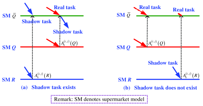
Figure 7: The shadow and real tasks

From the two supermarket models $Q$ and $R$, we construct a new supermarket model $\overline{Q}$ with shadow customers such that at environment state pair $\left(i,j\right)$, each arrival time in the supermarket model $\overline{Q}$ is the same time as that in the supermarket model $R$, while each departure time is the same time as that in supermarket model $Q$. Based on this, we can set up a coupling between the two supermarket models $R$ and $Q$ by means of the supermarket model $\overline{Q}$.

For a supermarket model $S$ and for $k\geq 1,1\leq i\leq m_{A},1\leq i\leq m_{B},x\geq 0,$ we define

$$\psi_{x}^{\left(i,j\right)}(S,t)=\sum_{n=1}^{N}\left[l_{n}^{\left(i,j\right)}(S,t)-x\right]_{+},$$

where $l_{n}^{\left(i,j\right)}(S,t)$ is the queue length of the $n$th server with environment state pair $\left(i,j\right)$ at time $t$, and $[y]_{+}=\max(y,0)$.

The following lemma gives a useful property of $\psi_{x}^{\left(i,j\right)}(S,t)$ for the two supermarket models $\overline{Q}$ and $R$.

Lemma 4

If $\psi_{y}^{\left(i,j\right)}(R,t)\leq\psi_{y}^{\left(i,j\right)}(\overline{Q},t)$ for all $y$ and $\psi_{x}^{\left(i,j\right)}(R,t)=\psi_{x}^{\left(i,j\right)}(\overline{Q},t)$, then

$$\#\left\{n:l_{n}^{\left(i,j\right)}(R,t)\leq x\right\}\leq\#\left\{n:l_{n}^{\left(i,j\right)}(\overline{Q},t)\leq x\right\}$$ (86)

and

$$\#\left\{n:l_{n}^{\left(i,j\right)}(R,t)\geq x\right\}\leq\#\left\{n:l_{n}^{\left(i,j\right)}(\overline{Q},t)\geq x\right\},$$ (87)

where $\#\left\{A\right\}$ means the number of elements in the set $A$.

Proof: If $\psi_{y}^{\left(i,j\right)}(R,t)\leq\psi_{y}^{\left(i,j\right)}(\overline{Q},t)$ for all $y$ and $\psi_{x}^{\left(i,j\right)}(R,t)=\psi_{x}^{\left(i,j\right)}(\overline{Q},t)$, then for $y=x+1$

$$-\psi_{x+1}^{\left(i,j\right)}(R,t)\geq-\psi_{x+1}^{\left(i,j\right)}(\overline{Q},t),$$

using $\psi_{x}^{\left(i,j\right)}(R,t)=\psi_{x}^{\left(i,j\right)}(\overline{Q},t)$ we get

$$\psi_{x}^{\left(i,j\right)}(R,t)-\psi_{x+1}^{\left(i,j\right)}(R,t)\geq\psi_{x}^{\left(i,j\right)}(\overline{Q},t)-\psi_{x+1}^{\left(i,j\right)}(\overline{Q},t).$$ (88)

Similarly, for $y=x-1$ we have

$$\psi_{x}^{\left(i,j\right)}(R,t)-\psi_{x-1}^{\left(i,j\right)}(R,t)\leq\psi_{x}^{\left(i,j\right)}(\overline{Q},t)-\psi_{x-1}^{\left(i,j\right)}(\overline{Q},t).$$ (89)

Since

$$\psi_{x}^{\left(i,j\right)}(S,t)=\sum_{n=1}^{N}\left[l_{n}^{\left(i,j\right)}(S,t)-x\right]_{+},$$

we obtain

$$\psi_{x}^{\left(i,j\right)}(S,t)-\psi_{x+1}^{\left(i,j\right)}(S,t)=\sum_{n=1}^{N}\left\{\left[l_{n}^{\left(i,j\right)}(S,t)-x\right]_{+}-\left[l_{n}^{\left(i,j\right)}(S,t)-\left(x+1\right)\right]_{+}\right\}.$$

To calculate $\psi_{x}^{\left(i,j\right)}(S,t)-\psi_{x+1}^{\left(i,j\right)}(S,t)$, we analyze the following two cases:

Case one: If $l_{n}^{\left(i,j\right)}(S,t)\leq x$, then $\left[l_{n}^{\left(i,j\right)}(S,t)-x\right]_{+}=\left[l_{n}^{\left(i,j\right)}(S,t)-\left(x+1\right)\right]_{+}=0$.

Case two: If $l_{n}^{\left(i,j\right)}(S,t)>x$, then $\left[l_{n}^{\left(i,j\right)}(S,t)-x\right]_{+}-\left[l_{n}^{\left(i,j\right)}(S,t)-\left(x+1\right)\right]_{+}=1$.

If $\sum_{n=1}^{N}\left\{\left[l_{n}^{\left(i,j\right)}(S,t)-x\right]_{+}-\left[l_{n}^{\left(i,j\right)}(S,t)-\left(x+1\right)\right]_{+}\right\}=k$, then $k$ is the number of servers whose queue length is bigger than $x$. That is $\#\left\{n:l_{n}^{\left(i,j\right)}(S,t)>x\right\}=k$. Hence, we obtain

$$\psi_{x}^{\left(i,j\right)}(S,t)-\psi_{x+1}^{\left(i,j\right)}(S,t) =\sum_{n=1}^{N}\left\{\left[l_{n}^{\left(i,j\right)}(S,t)-x\right]_{+}-\left[l_{n}^{\left(i,j\right)}(S,t)-\left(x+1\right)\right]_{+}\right\}$$

$$=\#\left\{n:l_{n}^{\left(i,j\right)}(S,t)>x\right\}.$$ (90)

It follows from (88) to (90) that

$$\#\left\{n:l_{n}^{\left(i,j\right)}(R,t)>x\right\}\geq\#\left\{n:l_{n}^{\left(i,j\right)}(\overline{Q},t)>x\right\},$$

this gives

$$\#\left\{n:l_{n}^{\left(i,j\right)}(R,t)\leq x\right\}\leq\#\left\{n:l_{n}^{\left(i,j\right)}(\overline{Q},t)\leq x\right\}.$$

Similarly, it follows from (89) to (90) that

$$\#\left\{n:l_{n}^{\left(i,j\right)}(R,t)>x-1\right\}\leq\#\left\{n:l_{n}^{\left(i,j\right)}(\overline{Q},t)>x-1\right\},$$

which follows

$$\#\left\{n:l_{n}^{\left(i,j\right)}(R,t)\geq x\right\}\leq\#\left\{n:l_{n}^{\left(i,j\right)}(\overline{Q},t)\geq x\right\}.$$

This completes the proof.  

The following lemma sets up the coupling between the two supermarket models $R$ and $\overline{Q}$, which is based on the arrival and departure processes.

Lemma 5

For the two supermarket models $R$ and $\overline{Q}$ and for $x,t\geq 0,1\leq i\leq m_{A},1\leq i\leq m_{B}$, we have

$$\psi_{x}^{\left(i,j\right)}(R,t)\leq\psi_{x}^{\left(i,j\right)}(\overline{Q},t).$$ (91)

Proof: To prove (91), we need to discuss the departure process and the arrival process, respectively.

(1) The departure process

Note that the two supermarket models $R$ and $\overline{Q}$ have the same initial state at $t=0$, thus (91) holds at time $t=0$.

In the departing process, it is easy to see from the above coupling that at environment state pair $\left(i,j\right)$, if given the server orders in supermarket models $\overline{Q}$ and $R$ according to the queue length of each server (including shadow tasks), then the customer departures always occur at the same order servers. For example, if the customer departure occurs from the server with the shortest queue length in supermarket model $\overline{Q}$, then a customer departure must also occur from the server with the shortest queue length in supermarket model $R$. Note that the customer departures will be lost either from an empty server or from one containing only shadow customers.

Let $D$ be a potential departure time at environment state pair $\left(i,j\right)$, and suppose that (91) holds for $t<D$. Then we hope to show that (91) holds for $t=D$.

Suppose that (91) does not hold at a departure point $D$. Then we have $\psi_{x}^{\left(i,j\right)}(R,D)>\psi_{x}^{\left(i,j\right)}(\overline{Q},D)$.

Since (91) holds for $t<D$, we get that $\psi_{x}^{\left(i,j\right)}(\overline{Q},D^{-})\leq\psi_{x}^{\left(i,j\right)}(R,D^{-})$. Based on this, we discuss the two cases: $\psi_{x}^{\left(i,j\right)}(\overline{Q},D^{-})=\psi_{x}^{\left(i,j\right)}(R,D^{-})$ and $\psi_{x}^{\left(i,j\right)}(\overline{Q},D^{-})<\psi_{x}^{\left(i,j\right)}(R,D^{-})$, and indicate how the two cases influence the departure process at time $D$.

Case one: If $\psi_{x}^{\left(i,j\right)}(\overline{Q},D^{-})=\psi_{x}^{\left(i,j\right)}(R,D^{-})$ and $\psi_{x}^{\left(i,j\right)}(R,D)>\psi_{x}^{\left(i,j\right)}(\overline{Q},D)$, then a departure at time $D$ makes that $\psi_{x}^{\left(i,j\right)}(R,D)$ does not change, while $\psi_{x}^{\left(i,j\right)}(\overline{Q},D)$ is diminished. Let $a$ and $b$ be the queue lengths at time $D$ in the two supermarket models $\overline{Q}$ and $R$, respectively. Then for $x=0,1,\ldots,a-1$, it is seen that

$$\psi_{x}^{\left(i,j\right)}(\overline{Q},D^{-})=\sum_{n=1}^{N}\left[l_{n}^{\left(i,j\right)}(\overline{Q},t)-x\right]_{+}$$

reduces $1$. Similarly, for $x=0,1,\ldots,b-1$,

$$\psi_{x}^{\left(i,j\right)}(R,D^{-})=\sum_{n=1}^{N}\left[l_{n}^{\left(i,j\right)}(R,t)-x\right]_{+}$$

also reduce $1$. Therefore, when $x$ is $b,b+1,\ldots,a-1$ (that is $b\leq x<a$), we have $\psi_{x}^{\left(i,j\right)}(R,D)>\psi_{x}^{\left(i,j\right)}(\overline{Q},D)$. However, when $\psi_{x}^{\left(i,j\right)}(\overline{Q},D^{-})=\psi_{x}^{\left(i,j\right)}(R,D^{-})$, both from that (86) holds for $t<D$ and from that the departure channels are at a coupling, it is clear that the condition: $\psi_{x}^{\left(i,j\right)}(R,D)>\psi_{x}^{\left(i,j\right)}(\overline{Q},D)$ for $b\leq x<a$, is impossible.

Case two: $\psi_{x}^{\left(i,j\right)}(R,D^{-})<\psi_{x}^{\left(i,j\right)}(\overline{Q},D^{-})$. In this case, when a customer departs the system, the two numbers $\psi_{x}^{\left(i,j\right)}(R,D^{-})$ and $\psi_{x}^{\left(i,j\right)}(\overline{Q},D^{-})$ have only two cases: Unchange and diminish $1$. Note that $\psi_{x}^{\left(i,j\right)}(R,D^{-})<\psi_{x}^{\left(i,j\right)}(\overline{Q},D^{-})$, we get that $\psi_{x}^{\left(i,j\right)}(R,D^{-})+1\leq\psi_{x}^{\left(i,j\right)}(\overline{Q},D^{-})$. Hence, we can not obtain that $\psi_{x}^{\left(i,j\right)}(R,D)>\psi_{x}^{\left(i,j\right)}(\overline{Q},D)$.

(2) The arrival process

In a similar way to the above analysis in ”(1) The departure process”, we discuss the coupling for the arriving process as follows.

Let $A=A_{k}^{\left(i,j\right)}$ be an arrival time. Then (91) holds for $t<A$. We hope to show that (91) holds for $t=A$.

This proof is similar to the above analysis in ”(1) The departure process”. Let $a$ and $b$ be the queue lengths at time $A$ in the two supermarket models $\overline{Q}$ and $R$, respectively. Then $\psi_{x}^{\left(i,j\right)}(R,A^{-})=\psi_{x}^{\left(i,j\right)}(\overline{Q},A^{-})$ holds for some $x$ for $a<x\leq b$. Thus, it follows from (87) that

$$\#\left\{n:l_{n}^{\left(i,j\right)}(R,A^{-})\geq x\right\}\leq\#\left\{n:l_{n}^{\left(i,j\right)}(\overline{Q},A^{-})\geq x\right\}$$

and

$$\#\left\{n:l_{n}^{\left(i,j\right)}(R,A^{-})\geq b\right\}\leq\#\left\{n:l_{n}^{\left(i,j\right)}(\overline{Q},A^{-})\geq a\right\}.$$

However, the condition: $\#\left\{n:l_{n}^{\left(i,j\right)}(R,A^{-})\geq b\right\}\leq\#\left\{n:l_{n}^{\left(i,j\right)}(\overline{Q},A^{-})\geq a\right\}$, is impossible, because it follows from the above coupling that for $a<x\leq b$

$$\#\left\{n:l_{n}^{\left(i,j\right)}(R,A^{-})\geq b\right\}>\#\left\{n:l_{n}^{\left(i,j\right)}(\overline{Q},A^{-})\geq a\right\}.$$

Since the queue length $a$ was chosen at the arrival time, it is seen that the queue length $a$ must exist in the supermarket model $\overline{Q}$. In this case, we get that $\#\left\{n:l_{n}^{\left(i,j\right)}(\overline{Q},A^{-})=a\right\}\geq 1$. Therefore, this leads to a contradiction.

Note that there are some shadow customers in supermarket model $\overline{Q}$, the shadow customers do not affect the queue lengths in the supermarket model $\overline{Q}$ at the arrival time $A_{k}^{\left(i,j\right)}(Q)$, thus (91) holds. This completes the proof.  

The following lemma provides the coupling between the two supermarket models $Q$ and $R$, which is based on the arrival and departure processes.

Lemma 6

In the two supermarket models $Q$ and $R$, for $k>0,1\leq i\leq m_{A},1\leq j\leq m_{B}$ we have

$$D_{k}^{\left(i,j\right)}\left(R\right)\leq D_{k}^{\left(i,j\right)}\left(Q\right)$$ (92)

and

$$A_{k}^{\left(i,j\right)}\left(R\right)\leq A_{k}^{\left(i,j\right)}\left(Q\right).$$ (93)

Proof: Using the above coupling, now we continue to discuss the two supermarket models $Q$ and $R$.

Note that the two supermarket models $Q$ and $R$ have the same parameters $N,m,c_{i,j},d_{i,j},\mu_{i}$ for $1\leq i,j\leq m$ and the same initial state at $t=0$, the departure or arrival of the $k$th customer and the Markov environment process in the supermarket model $Q$ correspond to those in the supermarket model $R$. This ensures that if (92) holds for the departure process up to a given time, then so does (93) for the arrival process up to that time.

Now, we use (91) to prove (92).

Suppose that (92) is false, that is, $D_{k}^{\left(i,j\right)}\left(R\right)>D_{k}^{\left(i,j\right)}\left(Q\right)$. Then the number of customer departures before time $D$ from the supermarket model $R$ must be the same as that in the supermarket model $\overline{Q}$. Since the arrivals in the two supermarket models $R$ and $\overline{Q}$ occur at the same times, there must be the same total number of customers in the two supermarket models $R$ and $\overline{Q}$. Hence, $\psi_{0}^{\left(i,j\right)}(R,D^{-})=\psi_{0}^{\left(i,j\right)}(\overline{Q},D^{-})$. But, it is seen from (86) that the number of servers with non-zero queue length in the supermarket model $\overline{Q}$ is bigger than that in the supermarket model $R$, this indicates that the number of servers with empty server in the supermarket model $\overline{Q}$ is less than that in the supermarket model $R$. Therefore, if a departure occurs in the supermarket model $\overline{Q}$, then there must be a departure in the supermarket model $R$. On the contrary, if a departure occurs in the supermarket model $R$, then it is possible not to have a departure in the supermarket model $\overline{Q}$. Note that the departure time in the supermarket model $\overline{Q}$ is the same as that in the supermarket model $Q$, hence the departure time in the supermarket model $R$ is earlier than that in the supermarket model $Q$, that is, $D_{k}^{\left(i,j\right)}\left(R\right)\leq D_{k}^{\left(i,j\right)}\left(Q\right)$. This leads to a contradiction of the assumption $D_{k}^{\left(i,j\right)}\left(R\right)>D_{k}^{\left(i,j\right)}\left(Q\right)$. Hence (92) holds. Similarly, we can prove (93). This completes the proof.  

Proof of Theorem 3: Using the lemma 6, we know that $D_{k}^{\left(i,j\right)}\left(R\right)\leq D_{k}^{\left(i,j\right)}\left(Q\right)$ and $A_{k}^{\left(i,j\right)}\left(R\right)\leq A_{k}^{\left(i,j\right)}\left(Q\right)$. This indicates that for any two corresponding servers in the two supermarket models $Q$ and $R$, the arrival and departure times in the supermarket model $R$ are earlier than those in the supermarket model $Q$. Hence, the queue length of any server in the supermarket model $R$ is shorter than that of the corresponding server in the supermarket model $Q$. This shows that the total number of customers in the supermarket model $R$ is no greater than the total number of customers in the supermarket model $Q$ at time $t\geq 0$. Based on this, we obtain a coupling between the processes $\{U_{Q}^{\left(N\right)}\left(t\right)\}$ and $\{U_{R}^{\left(N\right)}\left(t\right)\}$: For all $t\geq 0$, the total number of customers in the supermarket model $R$ is no greater than that in the supermarket model $Q$. This completes the proof.  

Quan-Lin Li is Full Professor in School of Economics and Management Sciences, Yanshan University, Qinhuangdao, China. He received the Ph.D. degree in Institute of Applied Mathematics, Chinese Academy of Sciences, Beijing, China in 1998. He has published a book (Constructive Computation in Stochastic Models with Applications: The RG-Factorizations, Springer, 2010) and over 40 research papers in a variety of journals, such as, Advances in Applied Probability, Queueing Systems, Stochastic Models, European Journal of Operational Research, Computer Networks, Performance Evaluation, Discrete Event Dynamic Systems, Computers & Operations Research, Computers & Mathematics with Applications, Annals of Operations Research, and International Journal of Production Economics. His main research interests concern with Queueing Theory, Stochastic Models, Matrix-Analytic Methods, Manufacturing Systems, Computer Networks, Network Security, and Supply Chain Risk Management.

John C.S. Lui (M 93-SM 02-F 10) was born in Hong Kong. He received the Ph.D. degree in computer science from the University of California, Los Angeles, 1992. He is currently a Professor with the Department of Computer Science and Engineering, The Chinese University of Hong Kong (CUHK), Hong Kong. He was the chairman of the Department from 2005 to 2011. His current research interests are in communication networks, network/system security (e.g., cloud security, mobile security, etc.), network economics, network sciences (e.g., online social networks, information spreading, etc.), cloud computing, large-scale distributed systems, and performance evaluation theory. Professor Lui is a Fellow of the Association for Computing Machinery (ACM), a Fellow of IEEE, a Croucher Senior Research Fellow, and an elected member of the IFIP WG 7.3. He serves on the Editorial Board of IEEE/ACM Transactions on Networking, IEEE Transactions on Computers, IEEE Transactions on Parallel and Distributed Systems, Journal of Performance Evaluation and International Journal of Network Security. He received various departmental teaching awards and the CUHK Vice-Chancellor s Exemplary Teaching Award. He is also a co-recipient of the IFIP WG 7.3 Performance 2005 and IEEE/IFIP NOMS 2006 Best Student Paper Awards.

Figure 8:

References

- [1] Bramson M, Lu Y, Prabhakar B (2010) Randomized load balancing with general service time distributions. In: Proceedings of the ACM SIGMETRICS International Conference on Measurement and Modeling of Computer Systems, pp 275–286
- [2] Bramson M, Lu Y, Prabhakar B (2012) Asymptotic independence of queues under randomized load balancing. Queueing Syst 71:247–292
- [3] Bramson M, Lu Y, Prabhakar B (2013) Decay of tails at equilibrium for FIFO join the shortest queue networks. Ann Appl Probab 23:1841–1878
- [4] Ethier SN, Kurtz TG (1986) Markov Processes: Characterization and Convergence. John Wiley & Sons, New York
- [5] Graham C (2000) Kinetic limits for large communication networks. In: N. Bellomo and M. Pulvirenti (eds.) Modelling in Applied Sciences. Birkhäuser, pp 317–370
- [6] Graham C (2000) Chaoticity on path space for a queueing network with selection of the shortest queue among several. J Appl Probab 37:198–201
- [7] Graham C (2004) Functional central limit theorems for a large network in which customers join the shortest of several queues. Probab Theory Relat Fields 131:97–120
- [8] Jacquet P, Vvedenskaya ND (1998) On/off sources in an interconnection networks: Performance analysis when packets are routed to the shortest queue of two randomily selected nodes. Technical Report N0 3570, INRIA Rocquencourt, Frence
- [9] Jacquet P, Suhov YM, Vvedenskaya ND (1999) Dynamic routing in the mean-field approximation. Technical Report N0 3789, INRIA Rocquencourt, Frence
- [10] Kurtz TG (1981) Approximation of Population Processes. SIAM
- [11] Li QL (2010) Constructive Computation in Stochastic Models with Applications: The -Factorizations. Springer and Tsinghua Press
- [12] Li QL (2011) Super-exponential solution in Markovian supermarket models: Framework and challenge. Available: arXiv:1106.0787
- [13] Li QL (2014) Tail probabilities in queueing processes. Asia-Pacific Journal of Operational Research 31:1–31 (No. 2)
- [14] Li QL, Cao J (2004) Two types of -factorizations of quasi-birth-and-death processes and their applications to stochastic integral functionals. Stochastic Models 20:299-340
- [15] Li QL, Dai G, Lui JCS, Wang Y (2013) The mean-field computation in a supermarket model with server multiple vacations. Discrete Event Dyn Syst, Available in Publishing Online: November 8, 2013, Pages 1–50
- [16] Li QL, Lui JCS (2010) Doubly exponential solution for randomized load balancing models with Markovian arrival processes and PH service times. Available: arXiv:1105.4341
- [17] Li QL, Lui JCS, Wang Y (2011) A matrix-analytic solution for randomized load balancing models with PH service times. In: Performance Evaluation of Computer and Communication Systems: Milestones and Future Challenges. Lecture Notes in Computer Science, vol 6821, pp 240–253
- [18] Luczak MJ, McDiarmid C (2006) On the maximum queue length in the supermarket model. Ann Probab 34:493–527
- [19] Luczak MJ, McDiarmid C (2007) Asymptotic distributions and chaos for the supermarket model. Electron J Probab 12:75–99
- [20] Luczak MJ, Norris JR (2005) Strong approximation for the supermarket model. Ann Appl Probab 15:2038–2061
- [21] Martin JB (2001) Point processes in fast Jackson networks. Ann Appl Probab 11:650–663
- [22] Martin JB, Suhov YM (1999) Fast Jackson networks. Ann Appl Probab 9:854–870
- [23] Mitzenmacher MD (1996) The Power of Two Choices in Randomized Load Balancing. PhD Thesis, Department of Computer Science, University of California at Berkeley, USA
- [24] Mitzenmacher MD (1999) On the analysis of randomized load balancing schemes. Theory Comput Syst 32:361–386
- [25] Mitzenmacher MD, Richa A, Sitaraman R (2001) The power of two random choices: A survey of techniques and results. In: Handbook of randomized computing, vol 1, pp 255–312
- [26] Mitzenmacher MD, Upfal E (2005) Probability and Computing: Randomized Algorithms and Probabilistic Analysis. Cambridge University Press
- [27] Neuts MF (1981) Matrix-Geometric Solutions in Stochastic Models: An Algorithmic Approach. Johns Hopkins University Press
- [28] Neuts MF (1989) Structured Stochastic Matrices of Type and Their Applications. Marcel Decker Inc., New York.
- [29] Suhov YM, Vvedenskaya ND (2002) Fast Jackson Networks with Dynamic Routing. Probl Inf Transm 38:136–153
- [30] Turner SRE (1996) Resource Pooling in Stochastic Networks. Ph.D. Thesis, Statistical Laboratory, Christ’s College, University of Cambridge
- [31] Turner SRE (1998) The effect of increasing routing choice on resource pooling. Probability in the Engineering and Informational Sciences 12:109–124
- [32] Vvedenskaya ND, Dobrushin RL, Karpelevich FI (1996) Queueing system with selection of the shortest of two queues: An asymptotic approach. Probl Inf Transm 32:20–34
- [33] Vvedenskaya ND, Suhov YM (1997) Dobrushin’s mean-field approximation for a queue with dynamic routing. Markov Processes and Related Fields 3:493–526
- [34] Vvedenskaya ND, Suhov YM (2005) Dynamic routing queueing systems with vacations. Information Processes, Electronic Scientific Journal. The Keldysh Institute of Applied Mathematics. The Institute for Information Transmission Problems, vol 5, pp 74–86