$\mathcal{PT}$-Symmetric Dimers with Time-Periodic Gain/Loss Function

Abstract

$\mathcal{PT}$-symmetric dimers with a time-periodic gain/loss function in a balanced configuration where the amount of gain equals that of loss are investigated analytically and numerically. Two prototypical dimers in the linear regime are investigated: a system of coupled classical oscillators, and a Schrödinger dimer representing the coupling of field amplitudes; each system representing a wide class of physical models. Through a thorough analysis of their stability behaviour, we find that turning on the coupling parameter in the classical dimer system, leads initially to decreased stability but then to re-entrant transitions from the exact to the broken $\mathcal{PT}-$phase and vice versa, as it is increased beyond a critical value. On the other hand, the Schrödinger dimer behaves more like a single oscillator with time-periodic gain/loss. In addition, we are able to identify the conditions under which the behaviour of the two dimer systems coincides and/or reduces to that of a single oscillator.

1 Introduction

Artificial materials with engineered properties have recently attracted a lot of attention. A well-known paradigm is the parity-time (${\cal PT}$) symmetric systems, whose properties rely on a delicate balance between gain and loss. The ideas and notions of ${\cal PT}-$symmetric materials, which do not separately obey the parity ($\cal P$) and and time ($\cal T$) symmetries, instead exhibiting a combined ${\cal PT}$ symmetry, have their roots in non-Hermitian quantum mechanics [1]. The theory has been extended to optical lattices [2, 3], and the predicted ${\cal PT}-$symmetry breaking as well as other properties have been experimentally observed in optical [4, 5, 6, 7, 8] and microresonator [9] systems. The theory subsequently evolved to include nonlinear lattices [10] and oligomers [11, 12]. The application of these ideas in electronic circuits [13, 14], provides a convenient platform for testing ${\cal PT}-$related ideas within the framework of easily accessible experimental configurations. Also, the construction of ${\cal PT}-$metamaterials, reliant on gain and loss-providing components, has been recently suggested [15, 16]. ${\cal PT}-$symmetric systems can migrate from the exact into the broken phase as the parameters of the system are varied. In the exact phase, ${\cal PT}-$symmetric systems have real eigenvalues, and thus propagating modes as well as bound states, despite being non-Hermitian. One essential difference from conventional systems is that the total energy, instead of being conserved, oscillates because the eigenmodes are not orthogonal. Another consequence of the non-orthogonality of the eigenmodes is non-reciprocal propagation [5], an asymmetry in the propagation in the two channels, even as the initial conditions are reversed. In the broken phase, the energy increases exponentially, and the propagation is unstable: amplified under gain or decaying with loss. The band structure of the system in the broken phase acquires imaginary components for some values of the wavevector [3, 5, 6]. Experimentally, grating structures have been synthesized and used to demonstrate greatly enhanced or reduced reflection in the broken phase [6, 7], paving the way for more extensive studies of these remarkable phenomena, and later, for the design of new devices exploiting them. Recently, a ${\cal PT}-$symmetric coherent perfect absorber was realized which can completely absorb light in its exact phase [17].

In the present work, two different ${\cal PT}-$symmetric models are investigated: a system consisting of two coupled linear oscillators (classical dimer), and a linear Schrödinger dimer (LSD). Both systems include terms providing gain and loss, which render them ${\cal PT}-$symmetric. In most previous works’ implementation, the gain/loss parameter remains constant in time, although recently a time-varying gain/loss function has been implemented in coupled fibre loops [6]. More generalized ${\cal PT}-$symmetric dimer models in various contexts, that include cubic or other nonlinearities and constant gain/loss functions, have been also investigated theoretically [18, 19, 20, 21, 22, 23, 24, 25, 26]. Moreover, the addition of a second spatial dimension in the nonlinear Schrödinger dimer, which activates spatial dispersion, results in the appearence of solitons and rogue waves as in ${\cal PT}-$symmetric dual-core waveguides [27, 28]. In extended nonlinear ${\cal PT}-$symmetric lattices, on the other hand, the existence of localized excitations in the form of discrete solitons [29] and discrete breathers [15] has been demonstrated. In the present work, a periodic in time gain/loss function having an opposite effect on the two components is considered. When averaged over one period, the amount of gain equals the loss in each component. This time-dependence of the gain/loss function introduces yet another parameter into the problem, and this results in multiple ${\cal PT}$ transitions from the exact phase, where stable propagation exists, to the broken phase, where all solutions diverge. In the following we describe the two above-mentioned systems and discuss the methods used in their analysis. The next section is devoted to the ${\cal PT}-$symmetric classical dimer, while a description of the ${\cal PT}-$symmetric LSD is given in Section 3. The conclusions are presented in the last section.

2 Linear $\mathcal{PT}$-Symmetric Classical Dimer

A $\mathcal{PT}$-symmetric dimer comprising two linear classical oscillators with a time-periodic gain/loss function $\gamma=\gamma(t)$ with $t$ being the temporal variable, is modeled by the equations

$$\ddot{x}_{1}+2\gamma(t)\dot{x}_{1}+\omega_{0}^{2}x_{1} =k(x_{2}-x_{1})$$ (1)

$$\ddot{x}_{2}-2\gamma(t)\dot{x}_{2}+\omega_{0}^{2}x_{2} =k(x_{1}-x_{2}),$$ (2)

where $x_{1}$ and $x_{2}$ are the longitudinal-mode displacements from equilibrium of the first and second oscillator, respectively, $\omega_{0}$ is their (common) eigenfrequency, $k$ is the coupling constant, and the overdots denote differentiation with respect to time $t$. Note that the commonly-appearing damping factor, which acts on the velocity of each oscillator, has been replaced by the gain/loss function $\gamma(t)$; also note that the signs in front of $\gamma(t)$ are opposite in the two equations.

A particularly simple form of $\gamma(t)$ which allows the reduction of Eqs. (1) and (2) to an area-preserving mapping for discrete time is the following piece-wise linear gain/loss function

$$\gamma(t)=\left\{\begin{array}[]{ll}+\gamma_{0}&\mbox{if $0\leq t<\tau_{1}$};\\ -\gamma_{0}&\mbox{if $\tau_{1}\leq t<\tau_{2}$}\end{array}\right.$$ (3)

where $\tau_{1}+\tau_{2}\equiv T$, the period of $\gamma(t)$, and the constant $\gamma_{0}$ is defined as positive real number ($\gamma_{0}>0$). Using Eq. (3), we have, say for the first oscillator, loss in the first part of the cycle ($\tau_{1}$ time units) and gain in the second part of the cycle ($\tau_{2}$ time units). With this form of $\gamma(t)$, Eqs. (1) and (2) are easily solvable in each part of the cycle separately. Note that for the dimers having an averaged balanced configuration, $\tau_{1}$ and $\tau_{2}$ need not be equal; in the present work however, the case of $\tau_{1}=\tau_{2}=\tau$ is investigated. The solution of the $x_{i}$, $i=1,2$, in each half-period $\tau\equiv T/2$ of $\gamma(t)$ is of the form:

$$x_{i}(t)=c_{1}\mathrm{e}^{r_{1}t}+c_{2}\mathrm{e}^{r_{2}t}+c_{3}\mathrm{e}^{r_{3}t}+c_{4}\mathrm{e}^{r_{4}t}$$ (4)

for generally complex constants $r_{j}$, $c_{j}$, $j=1,...,4$, that can be expressed analytically as a function of the initial conditions (at time $t=0$). Then, the coefficients of $x_{1}(t=0)\equiv x_{1,0}$, $\dot{x}_{1}(t=0)\equiv\dot{x}_{1,0}$, $x_{2}(t=0)\equiv x_{2,0}$, and $\dot{x}_{2}(t=0)\equiv\dot{x}_{2,0}$ are collected and used to construct the propagation matrix $M_{0\rightarrow\tau}$ ($M_{\tau\rightarrow T}$) for the first (second) half of the period $T$ of the gain/loss function, using the same method as in Ref. [16]. The relation of the amplitudes and the velocities at time $t=0$ with those at time $t=T$ can then be written in the matrix form

$$\begin{pmatrix}x_{1}\\ \dot{x}_{1}\\ x_{2}\\ \dot{x}_{2}\end{pmatrix}=\underline{\underline{M}}_{0\rightarrow\tau}(\tau)\underline{\underline{M}}_{\tau\rightarrow T}(\tau)=\underline{\underline{M}}_{G/L}(\tau)\begin{pmatrix}x_{1,0}\\ \dot{x_{1,0}}\\ x_{2,0}\\ \dot{x_{2,0}}\end{pmatrix}$$ (5)

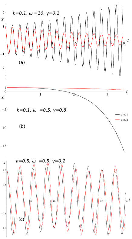
Figure 1: (Color online) Oscillation amplitude for constant in time gain/loss function $\gamma$, for the initial conditions $(x_{1},\dot{x}_{1},x_{2},\dot{x}_{2})=(1,0,1,0)$, and (a) $\omega_{0}>\gamma$ (both oscillators underdamped); (b) $\omega_{0}<\gamma$ (both oscillators overdamped); (c) $\omega_{0}<\gamma$. In this case the first oscillator is subject to gain and the second is subject to loss for all times. The motion is unstable in (a) and (b), while it is stable in (c).

2.1 Constant gain/loss function

For constant $\gamma$ the amplitudes of the oscillators for various cases are shown in Fig. 1. Both oscillators start with amplitude equal to unity and zero velocity, and the first oscillator is considered to have gain while the second one has loss. The variable $\tau$ here is infinity and the horizontal shows the real time. Although such a characterization is strictly valid only for $k=0$, the first case, (a), where $\omega_{0}>\gamma$, is termed ‘underdamped’ in order to connect the behaviour to the single-oscillator problem studied in [16], where the effective frequency, modified by $\gamma$, is real and leads to oscillatory motion, while case (b), where $\omega_{0}<\gamma$, is called ‘overdamped’, shows monotonic behaviour. In case (c) the motion is marginally-stable as it is stabilized by a sufficiently large $k$. Regions of stability as a result of nonzero $k$ can be found in either $\omega_{0}>\gamma$ or $\omega_{0}<\gamma$. This is not only clear from the solutions themselves, but from an analysis of the eigenvalues of the propagation matrix $M_{G/L}$, as will be discussed later in Sec. 2.2. The stability behaviour under constant gain/loss has already been discussed in Ref. [13], where a system very similar to that described by Eqs. (1) and (2) was studied theoretically, and it was implemented using electric circuits containing active-gain/loss components. In that study, the ratio of mutual to self-inductances of the two components comprising the $\mathcal{PT}$-symmetric dimer is related to the coupling $k$ here. However, no quantitative comparisons can be made between the two models due to different parametrization. In our model, Eqs. (1) and (2), from the analysis of the eigenfrequencies the stability condition for $\gamma$ constant in time is found to be

$$\gamma\leq\sqrt{\frac{1}{2}\left(k+\omega_{0}^{2}\right)-\frac{1}{2}\sqrt{2k\omega_{0}^{2}+\omega_{0}^{4}}}.$$ (6)

A phase diagram showing how nonzero $k$ stabilizes the motion in the constant $\gamma$ case is shown in Fig. 2a. The limit $k\rightarrow 0$ in the constant $\gamma$ system gives the result of instability except for $\gamma=0$, although this is a fictitious result due to the ambiguities inherent in the mapping of the dimer onto an uncoupled system (Sec. 2.3).

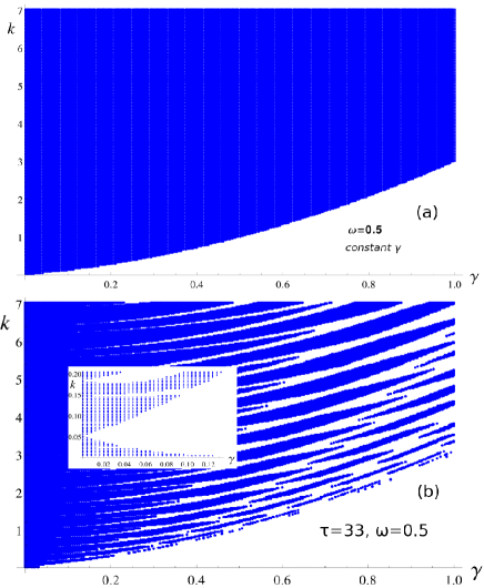
Figure 2: Stability phase diagram on the $k-\gamma$ parameter space for (a) constant gain/loss function $\gamma$; (b) time-dependent $\gamma=\gamma(t)$ with half-period $\tau=33$. The inset in (b) shows the stability in the low-$k$ region which is not present in the case of constant $\gamma$. The shaded (blank) regions correspond to stable (unstable) oscillations.

2.2 Time-periodic gain/loss and stability criterion

When the gain/loss function varies in time, there are changes in the stability behaviour. We have a reduced phase space for stability in the ‘underdamped’ region $\omega_{0}>\gamma$ and an increased phase space in the ‘overdamped’ region $\omega_{0}<\gamma$. Fig. 2, shows an example of the stabilizing effect of the coupling parameter $k$, something also noted experimentally in Ref. [6]. That study examined the $\mathcal{PT}$ threshold of two coupled waveguides subject to an opposing alternating $\gamma(t)$ -albeit with a fixed half-period $\tau$- while the real part of the $\mathcal{PT}$ potential, implemented as a time-varying phase factor, was adjusted. Unlike in the present model, their coupling parameter was also made to vary in time. Fig. 2b shows how introducing a time variation in $\gamma$ results in decreased stability in some regions and increased stability in others as compared with the case of constant $\gamma$ (inset).

Figure 3: Magnitudes $\left|\lambda\right|$ of the four eigenvalues as a function of the gain-loss oscillation half-period $\tau$ (a) for $k=0$ and $\omega=1.4$. Purple and Blue curves respectively: $\gamma=1.7$ and 1.5 (overdamped), black and red curves: $\gamma=1.3$ and 1 respectively (underdamped). Two eigenvalues drop below and two go above unity in the unstable regions. There is a qualitative correspondence to the behaviour of the eigenvalues in the overdamped and underdamped cases of linear Schrödinger dimer system, where $V$ replaces $\omega_{0}$. In (b), the parameters are $k=0.11$, $\omega_{0}$=1.4, and $\gamma=0.8$.

The stability points (marginally-stable oscillations for $x_{1}(t)$ and $x_{2}(t)$) occur when the (complex) eigenvalues of $M_{G/L}$ all simultaneously have the absolute value of unity. There was no other type of stability present; for no parameters were the eigenvalues simultaneously less than unity, which would have implied asymptotic stability (decaying to zero). In the regions of instability, two eigenvalues drop below while the other two go above unity (Fig. 3). Such oval-like structures appear in other studies of stability in $\mathcal{PT}$ systems [3, 13]. The instability onset is not as sharp as Fig. 3 seems to indicate; the motion will be bounded by some larger magnitudes than the initial value for values of $\tau$ below or above the unstable region, but the oscillation will still be bounded.

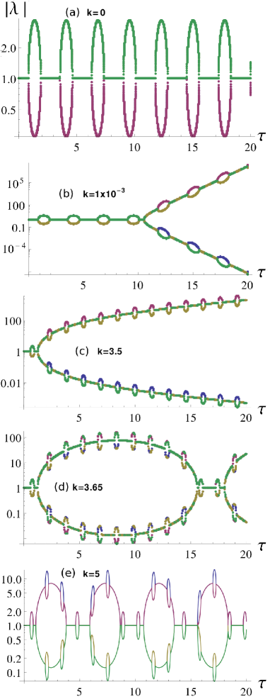
Figure 4: Magnitudes of the four eigenvalues for the propagation matrix $M_{G/L}$ in Eq. 5 for different values of the coupling $k$, as $\tau$ is varied. The values of $\omega_{0}$ and $\gamma$ are fixed at 1.4 and 0.8 respectively.

2.3 Effect of intra-dimer coupling

The full analytical expansion for the eigenvalues of $M_{G/L}$ in Eq. 5 is extremely complex while series expansions yield little insight as due to the correlation of the different variables, the convergence properties of any expansion are very complicated. If the limits leading to Fig. 2, where $k=0$ appears to lead to instability, are taken in reverse, with the limit $\tau\rightarrow\infty$ of the $k=0$ system taken, the result is indeterminate: neither stable nor unstable as discussed later at the beginning of Sec. 2.3 and as seen in Fig. 4a and Fig. 5. Lastly, a prediction of total stability for $\omega_{0}>\gamma$ and instability for $\omega_{0}<\gamma$ arises if a path such as that in Fig. 7c$\rightarrow$a, where $\gamma$ is fixed while $\omega_{0}$ is varied, is taken. Essentially, by choosing such a path, the periodicity with variable $\omega_{0}$ of the stripes reduces to zero, yielding the identity operation.

Likewise, the single oscillator with constant nonzero $\gamma$ is everywhere unstable, but performs according to Fig. 7a if $\tau$ is made to approach infinity while $\omega_{0}$ is varied for fixed $\gamma$, again because the periodicity of the $\mathcal{PT}$ symmetry-breaking stripes reduces to zero. On the other hand, the approach $\tau\rightarrow\infty$ for fixed $\omega_{0}$ and $\gamma$ is indeterminate as in Fig. 4a. Thus, we may reconcile the $k=0$ limit of the dimer with the behaviour of the single oscillator if the limits are chosen in a particular sequence.

The approaches $k\rightarrow 0,$ $\tau\rightarrow\infty,$ and $\gamma\rightarrow\omega_{0}$ are correlated amongst themselves and a mapping for a consistent (path-independent) unified approach from the dimer to the single-oscillator is currently being sought. Even numerically, the reduction of the coupled system to one of the phase diagrams of the single-oscillator is not valid for all paths towards the double limit $k\rightarrow 0$, and $\tau\rightarrow\infty,$ which is essentially undefined. Keeping this in mind, we explain below exactly how our calculations were performed for the limiting cases.

2.3.1 Zero coupling limit, $k$=0

In studying the case of $k=0$ or no coupling between oscillators, we choose to refer to the solution of a single oscillator [16], because the system of two oscillators does not in general reduce to that of one oscillator in the limit $k\rightarrow 0$, as it depends on the path taken. In the case of a single oscillator, there is a periodic set of stable trajectories for the underdamped limit $\omega_{0}>\gamma$ for all values of $\tau$. In this limit, the onset and/or end of the instabilities occurs periodically where [16]

$$\cos{(2\delta\tau_{crit})}=\left(\frac{2\gamma^{2}}{\omega_{0}^{2}}-1\right),$$ (7)

where $\delta=\sqrt{\omega_{0}^{2}-\gamma^{2}}$. For the overdamped ($\omega_{0}<\gamma$) case, there is only one solution to Eq. 7: $\tau_{crit}=\arccos{(\gamma/\omega_{0})}/\delta$, and the bifurcation in the magnitude of the eigenvalues is permanent beyond this point as it does not close in over itself (purple and blue curves in Fig. 3a). For values of $\gamma$ below $\omega_{0}$ the bifurcations close in over themselves and periodically repeat following Eq. 7, while the width and height of the unstable regions decreases with the value of $\gamma/\omega_{0}$. Finally, in the limit $\omega_{0}\gg\gamma$ the splitting of the eigenvalue magnitudes in the unstable regions (size of the bubbles) is reduced to zero whereupon we recover the undamped limit of conventional stability.

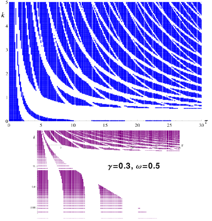
Figure 5: Stability phase diagram on the $k-\tau$ parameter plane for the linear classical dimer for constant $\gamma=0.3$ and $\omega_{0}=0.5.$ The lower plot is the same as the upper plot but with the vertical axis using a log scale in order to highlight the low$-k$ regime. The shaded (blank) regions correspond to stable (unstable) oscillations.

Note that Eq. 7, for constant $\gamma$, or infinite $\tau$, can have a $\mathcal{PT}$-symmetry breaking transition across the line ${\omega_{0}}_{crit}=\gamma$ so the system can indeed reduce to the behaviour in Fig. 7a if the paths are chosen according to prescription outlined at the start of this section, of varying $\omega_{0}$ while holding the other parameters fixed, so that in Eq. 7 we have $\tau$ instead of $\tau_{crit}$ and ${\omega_{0}}_{crit}$ instead of ${\omega_{0}}$. On the other hand, the stability prediction of Eq. 7 is indeterminate for $\tau\rightarrow\infty$ (see e.g. Fig. 4a and 5 for $k=0$) as $\tau$ is varied. In addition to the ${\omega_{0}}_{crit}\rightarrow\gamma$ case of Eq. 7, a separate condition can be derived for when the limit $\omega_{0}\rightarrow\gamma$ (system parameters as opposed to phase boundary as in the previous paragraph) is taken at the outset. If this is done, then we have a $\mathcal{PT}$ symmetry-breaking point occurring at $\tau_{crit}=1/\gamma$. This is the cause of the peak which appears for small $\tau$ in Figs. 7 and 8.

2.3.2 Nonzero $k$

The effect of nonzero $k$ is to shorten the region in $\tau$ where periodic stability/instability regions can occur. This is clearly seen by comparing Figs. 4a-c. However, as $k$ becomes large, beyond the critical value which occurs between Fig. 4c and d, a new regime is reached: that of a very noisy but infinitely-periodic region of $\mathcal{PT}$-symmetry breaking and recovery (Fig. 4d-e). Similar to the $k=0$ case of ${\omega_{0}}_{crit}=\gamma+0^{+}$ where the bifurcation closes in on itself to produce an infinite series of $\mathcal{PT}$-symmetry breaking and recovery, here also, for a critical value $k=k_{crit}$, between the cases pictured in Fig. 4c and d, the bifurcation behaves in a similar manner, leading to the production of a more-complex series of superimposed bubbles. The small, more numerous bubbles, are due to the underdamping $\omega_{0}>\gamma$ while the large ones are due to $k>k_{crit}$.

Just as the $\omega_{0}\gg\gamma$ case for the uncoupled oscillators, depicted in the phase plots of Fig. 7, leads to increased stability, or a longer $\tau_{crit}$ (Eq. 7), here also, if we have infinitely-large $k$, then we will recover the regime of continuous, unbroken symmetry because the symmetry-breaking bubbles shrink to zero size. In addition, we see from Fig. 7 that increasing $\tau$ leads to greater stability for an underdamped system, as we can otherwise see from Fig. 5 where the density of stable regions increases for larger $\tau$. In the regime $\tau\rightarrow\infty$ and large $k$ the classical dimer system behaves as independent undamped harmonic oscillators, showing conventional rather than $\mathcal{PT}$-symmetric stability. Studying the overdamped, $\omega_{0}<\gamma$, system is of little interest as the $\mathcal{PT}$-symmetric region is confined to a smaller phase space in comparison with the underdamped system as the recoveries for $k$ larger than the critical value have only the larger $k$ bubbles since the smaller ones do not exist. Thus, while the plots in Fig. 4 reveal the mechanism (through the bifurcations closing in on themselves) by which $k$ influences the size of the region of periodic $\mathcal{PT}$-symmetry breaking and recoveries, the $k-\tau$ phase diagram in Fig. 5 depicts the overall result over all $k$ values. In both of these examples, Fig. 4 and  5, with $\gamma<\omega_{0},$ the qualitative behaviour is the same, even as the exact parameters differ. We find an infinite series of $\mathcal{PT}$-symmetry breaking/recoveries for $k\rightarrow 0$ while, as seen in Figs. 4a-c, the $\mathcal{PT}$-symmetry breaking/recovery range in $\tau$ is reduced as $k$ is increased, something which is especially evident from the lower plot of Fig. 5, until there is just one recovery (viz. large gap in the phase plot). Upon increasing $k$ further, the infinite series of $\mathcal{PT}$-symmetry breaking/recoveries is regained beyond a critical value of $k$.

3 Linear Schrödinger $\mathcal{PT}$-Symmetric Dimer

Systems of Schrödinger dimers have been studied widely in the context of optics, where $\mathcal{PT}$-symmetry phenomena can be realized experimentally using e.g. gratings or coupled waveguides providing alternating gain/loss. The dynamical behaviour of the Schrödinger $\mathcal{PT}$-symmetric dimer is governed by the equations

$$i\dot{\Psi}_{a} =-i\gamma\Psi_{a}+V\Psi_{b}$$ (8)

$$i\dot{\Psi}_{b} =+i\gamma\Psi_{b}+V\Psi_{a}$$ (9)

where $\Psi_{i}$ is the wavefunction at site $i$ ($i=a,b$), with $V$ being the coupling between the two sites, $\gamma=\gamma(t)$ is the gain/loss function given by Eq. (3), and the overdot denotes derivation with respect to the temporal variable. The (non-Hermitian) Hamiltonian used to derive Eqs. (8) and (9) is given by

$$\mathcal{H}=\begin{pmatrix}-i\gamma&V\\ V&i\gamma\end{pmatrix}.$$ (10)

For $\gamma=0$, Eqs. (8) and (9) form a completely integrable system; thus, the Hamiltonian $\mathcal{H}$ and the total probability (norm)

$$P=\sum_{i=a,b}\left|\Psi_{i}\right|^{2},$$ (11)

are conserved. For $\gamma\neq 0$ neither $P$ nor $\mathcal{H}$ are conserved but instead, they oscillate in time; however, a more complex conserved quantity still exists [30].

3.1 Constant gain/loss

In contrast with the case of classical oscillators (e.g. the single one or the dimer as in Fig. 1), where a constant $\gamma$ in the broken $\mathcal{PT}$-symmetry phase led to either underdamped or overdamped growth or decay, the growth or decay here is always monotonic. Indeed, in experiments on light intensity in coupled waveguides [5], it has been found that above the $\mathcal{PT}$ transition point the light propagates, exponentially amplified, through one particular waveguide irrespective of the initial conditions.

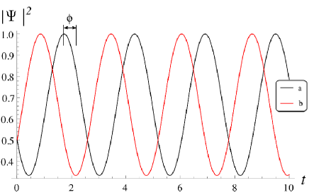
Figure 6: Magnitudes of the linear Schrödinger dimer wavefunctions for a constant nonzero damping $\gamma=0.7$, where oscillator $a$ is subject to gain and oscillator $b$ is subject to loss, for the initial conditions $(\Psi_{a},\Psi_{b})=(1/\sqrt{2},1/\sqrt{2})$ and $V$=1.4. The phase shift $\phi$, with respect to the phase difference $\pi$ corresponding to $\gamma=0,$ is shown.

For $V>\gamma$ the system is always $\mathcal{PT}$-symmetric (Fig. 7a), in stark contrast with the classical oscillator or dimer with $k=0$ where the theory predicts complete instability when the limit $\tau\rightarrow\infty$ is taken first (start of Sec. 2.3), and the magnitudes of the wavefunctions $\Psi_{a}(t)$ and $\Psi_{b}(t)$ of the coupled Schrödinger dimer undergo stable oscillations as they do in the exact $\mathcal{PT}$-symmetric phase of the classical dimer under constant gain/loss considered in Sec. 2.1. For $\gamma=0$ the wavefunction magnitudes are phase shifted with respect to each other by $\pi$ while when $\gamma\rightarrow V+0^{-}$ the phase difference asymptotically approaches zero. A phase shift of $\pi/2$ occurs at $\gamma=V/\sqrt{2}$. Fig. 6 shows an example of the phase difference between the two dimer components. Such phase delays between two eigenmodes of a coupled two-channel waveguide have been observed in experiments as $\gamma$ is varied [5] and they are attributed to the nonorthogonality of the modes. This constant phase delay is not present in the classical dimer system because non-zero $k$ is necessary for stability when the damping factor is constant; for nonzero $k$, as seen in Fig. 1c, the signals are chirped and eventually coalesce (at $t$=80). The time to coalescence approaches infinity as the $\mathcal{PT}$ transition is approached. The phase delay therefore can only be properly defined in the unstable regime, where for $k\rightarrow 0$ it is equal to $\pi/2$ right at the $\mathcal{PT}$ transition and zero far from the transition point $\tau_{crit}$, bearing in mind that for small $k$ the parameter space for stability is tiny (Fig. 2a). As with the case of broken $\mathcal{PT}-$symmetry in the overdamped limit of the classical dimer, for $V<\gamma$ all of the solutions diverge monotonically for a constant gain/loss $\gamma$.

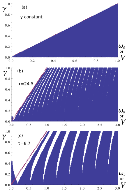
Figure 7: Stability phase diagram on the $\gamma-(V$ or $\omega_{0})$ parameter plane for the linear Schrödinger dimer, for (a) constant $\gamma$ and (b)-(c) oscillating $\gamma(t)$. Plots (b) and (c) may also correspond to the linear classical dimer with $k=0$ or to the single classical oscillator. (a) is achieved for the classical systems only in a specific regime as discussed in the text; otherwise it is blank. The shaded (blank) regions are stable (unstable). The purple dotted line shows the line $\gamma=V$ or $\omega_{0}$ which corresponds to the stable/unstable boundary in (a).

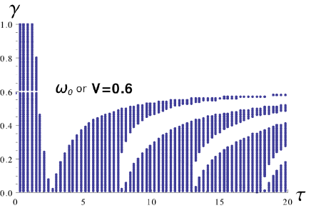
Figure 8: Stability phase diagram on the $\gamma-\tau$ parameter plane for the single oscillator, the classical dimer with $k=0$ or the linear Schrödinger dimer for ($V$ or $\omega_{0}$)=0.6. The shaded (blank) regions are stable (unstable).

3.2 Time-dependent gain/loss function

For the time-alternating $\gamma(t)$ of Eq. 3, $\Psi_{a}$ and $\Psi_{b}$ can be obtained analytically using the same methods described earlier, and a map that connects the $\Psi$s at times $t$ and $t+2\tau=t+T$ can be constructed so that

$$\begin{pmatrix}\Psi_{a}\\ \Psi_{b}\end{pmatrix}=\underline{\underline{M}}_{G/L}(\tau)\begin{pmatrix}{\Psi_{a,0}}\\ {\Psi_{b,0}}\end{pmatrix}$$ (12)

where $\Psi_{a,0}=\Psi_{a}(t=0)$ and $\Psi_{b,0}=\Psi_{b}(t=0)$. Examining the stability of the propagation matrix in Eq. 12, we find a direct correspondence with the behaviour of the single classical oscillator, mainly a regime $V<\gamma$ with diverging orbits beyond a certain $\tau$ where the instability criterion is established by the divergence of the eigenvalue magnitudes at

$$\tau_{crit}=\frac{\arccos{(\gamma/V)}}{\delta},$$ (13)

where $\delta=\sqrt{V^{2}-\gamma^{2}}$, and a regime with $V>\gamma$ containing periodic $\mathcal{PT}$-symmetry breaking/recoveries at

$$\cos{(2\delta\tau)}=\left(\frac{2\gamma^{2}}{V^{2}}-1\right).$$ (14)

Figure 9: Time-dependence of (a) the probabilities $\left|\Psi_{a}(t)\right|^{2}$ and $\left|\Psi_{b}(t)\right|^{2}$ for $\gamma<V$; (b) the total probability $P$ for $\gamma<V$; (c) the probability difference $\Delta\rho$ for $\gamma<V$ and $\gamma>V$. The initial conditions in all cases are $\Psi_{a}(0)=0$, $\Psi_{b}(0)=1$. In all cases shown the system is in the exact $\mathcal{PT}-$symmetric phase.

The overall $\gamma-\tau$ phase diagram is shown in Fig. 8 for $V$=0.6. For values of $\gamma<V$ there is an infinite series of $\mathcal{PT}-$symmetry breaking/recoveries while for $\gamma>V$ there is just a single, small region of stability. The probabilities for the oscillators $a$ and $b$ of the LSD in the exact $\mathcal{PT}$-symmetric phase are shown for a case of $\gamma<V$ in Fig. 9a, while their difference

$$\Delta\rho=\left|\Psi_{a}(t)\right|^{2}-\left|\Psi_{b}(t)\right|^{2}$$ (15)

is shown in Fig. 9c for both $\gamma<V$ and $\gamma>V$. While the probability of each component certainly is expected to oscillate in time, the non-conservation of the total probability is solely a feature of the non-Hermiticity of the system and it is more pronounced for a larger gain/loss parameter $\gamma$ (Fig. 9b). It occurs because when Hermiticity is violated, $\Psi_{a}$ and $\Psi_{b}$ no longer form an orthonormal basis of the non-Hermitian Hamiltonian in Eq. (10) [31]. The oscillation of $\Delta\rho$, on the other hand, is bounded in the exact $\mathcal{PT}$-symmetric phase (Fig. 9c) by $\pm 1$, irrespective of the value of $\gamma$.

4 Conclusions

We have investigated theoretically two $\mathcal{PT}$-symmetric dimer systems which are representative of two wide classes of models used for physical systems, and we have made comparisons to recent experiments covering both of these classes. In the first class considered, based on classical oscillators, all of the parameters are real and it is typically concerned with observables such as e.g. position, charge, etc., while the second, describing the time-evolution of field amplitudes, pertains to systems with generally complex parameters (e.g. index of refraction) and it is typically by optics experiments. ${\cal PT}-$symmetric dimer systems fabricated in a laboratory may be adequately modeled by one of the two models presented above. Thus, it is imperative to be able to predict their behavior in particular regions of parameter space. Phase diagrams, in which stability/instability regions corresponding to the exact/broken ${\cal PT}-$symmetric phase of the systems are shown, provide valuable information in that respect. In particular, they may be very helpful in identifying regions of the parameter space where stable solutions exist.

In a similar manner to how re-entrant ${\cal PT}-$symmetry transitions have been predicted in single classical oscillator with a periodically varied gain/loss parameter [16], the coupling parameter $k$ of the classical dimer induces another layer of ${\cal PT}-$symmetry transitions. For small values of $k$ the phase space for re-entrant ${\cal PT}-$symmetry transitions is reduced, while above a critical value $k_{crit}$ the transitions return and the system achieves greater stability as the coupling is increased beyond this point. Note that ${\cal PT}-$symmetry transitions as a function of the coupling strength have been recently observed in a coupled microresonator system [9]. The solutions of the two dimer models considered here display similar characteristics, such as a phase shift between the oscillator or field amplitudes correspondingly, as well as a non-conservation of oscillator or probability amplitude in the exact ${\cal PT}-$symmetric phase, and this distinguishes them from conventional (undamped) stability.

It is important to note that the two dimer models only reduce to the behaviour of a single classical oscillator, or ”zero-dimensional” ${\cal PT}-$symmetric system [16] that we chose as a benchmark here, under very specific and different conditions: paths, i.e. slices of phase space, and order of limits taken. As well, the two dimer systems may have very similar behaviour but they display subtle differences, particularly in the case of a constant gain/loss function $\gamma$ studied in great detail here. In order to make their behaviour coincide, limiting approaches need to be taken in a specific, and opposite sequence. The path-dependent and/or limiting behaviour is very important to be aware of in making correspondences between classical or wave-based models or in comparing or interpreting results from experiments belonging to the two different classes. As these simple dimer systems can be used as basic elements for the fabrication of larger networks comprised of dimers as in Refs. [6, 15, 29, 32], understanding the properties of the dimer elements is invaluable for deducing the properties of the system as a whole.

Acknowledgement

This work was partially supported by the European Union’s Seventh Framework Programme (FP7-REGPOT-2012-2013-1) under grant agreement n^o 316165, and by the Thales Project ANEMOS, co‐financed by the European Union (European Social Fund – ESF) and Greek national funds through the Operational Program ”Education and Lifelong Learning” of the National Strategic Reference Framework (NSRF) ‐ Research Funding Program: THALES. Investing in knowledge society through the European Social Fund.

References

- [1] Hook, D.W.: Non-Hermitian potentials and real eigenvalues. Ann. Phys. (Berlin) 524 (6-7), A106 (2012) (and references therein)
- [2] El-Ganainy, R., Makris, K.G., Christodoulides, D.N., Musslimani, Z.H.: Theory of coupled optical symmetric structures. Opt. Lett. 32, 2632–2634 (2007)
- [3] Makris, K.G., El-Ganainy, R., Christodoulides, D.N., Musslimani, Z.H.: Beam dynamics in symmetric optical lattices. Phys. Rev. Lett. 100, 103904 (2008)
- [4] Guo, A., Salamo, G.J., Duchesne, D., Morandotti, R., Volatier-Ravat, M., Aimez, V., Siviloglou, Christodoulides, D.N.: Observation of symmetry breaking in complex optical potentials. Phys. Rev. Lett. 103, 093902 (2009)
- [5] Rüter, C.E., Makris, K.G., El-Ganainy, R., Christodoulides, D.N., Segev, M., Kip, D.: Observation of parity-time symmetry in optics. Nature Physics 6, 192– (2010)
- [6] Regensburger, A., Bersch, C., Miri., M.-A., Onishchukov, G., Christodoulides, D. N., Peschel, U.: Parity-time synthetic photonic lattices. Nature 488, 167 (2012)
- [7] Feng, L., Xu, Y.L., Fegadolli, W.S., Lu, M.-H., Oliveira, J.E.B., Almeida, V.R., Chen, Y.-F., Scherer, A.: Experimental demonstration of a unidirectional reflectionless parity-time metamaterial at optical frequnecies. Nature Materials 12, 108-113 (2013)
- [8] Feng, L., Wong, Z.J., Ma, R., Wang, Y., Zhang, X.: Parity-time synthetic laser. arXiv:1405.2863
- [9] Peng, B., Özdemir, S.K., Lei, F., Monifi, F., Gianfreda, M., Long, G. L., Fan, S., Nori, F., Bender, C.M., Yang, L.: Parity–time-symmetric whispering-gallery microcavities. Nature Physics 10, 394-398 (2014)
- [10] Dmitriev, S.V., Sukhorukov, A.A., Kivshar, Y.S.: Binary parity-time-symmetric nonlinear lattices with balanced gain and loss. Opt. Lett. 35, 2976–2978 (2010)
- [11] Li, K., Kevrekidis, P.G.: symmetric oligomers: Analytical solutions, linear stability, and nonlinear dynamics. Phys. Rev. E 83, 066608 (2011)
- [12] D’Amroise, J.D., Kevrekidis, P.G., Lepri, S.: Asymmetric wave propagation through nonlinear symmetric oligomers. J. Phys. A: Math. Theor. 45, 444012 (2012)
- [13] Schindler, J., Li, A., Zheng, M.C., Ellis, F.M., Kottos, T.: Experimental study of active LRC circuits with symmetries. Phys. Rev. A 84, 040101(R) (2011)
- [14] Bender, N., Factor, S., Bodyfelt, J.D., Ramezani, H., Christodoulides, D.N., Ellis, F.M., Kottos, T,: Observation of asymmetric transport in structures with active nonlinearities. Phys. Rev. Lett. 110, 234101 (2013)
- [15] Lazarides, N., Tsironis, G.P.: Gain-driven discrete breathers in symmetric nonlinear metamaterials. Phys. Rev. Lett. 110, 053901 (2013)
- [16] Tsironis, G.P., Lazarides, N.: symmetric nonlinear metamaterials and zero-dimensional systems. Appl. Phys. A 115, 449–458 (2014)
- [17] Sun, Y., Tan, W., Li, H.-Q., Li, J., Chen, H.: Experimental demonstration of a coherent perfect absorber with phase transition. Phys. Rev. Lett. 112, 143903 (2014)
- [18] Ramezani, H., Kottos, T., El-Ganainy, R., Christodoulides, D.N.: Unidirectional nonlinear symmetric optical structures. Phys. Rev. A 82, 043803 (2010)
- [19] Benisty, H., Degiron, A., Lupu, A., De Lustrac, A., Chénais, S., Forget,i S., Besbes, M., Barbillon, G., Bruyant, A., Blaize, S., Lérondel, G.: Implementation of symmetric devices using plasmonics: principle and applications. Opt. Express 19, 18004 (2011)
- [20] Barashenkov, I.V., Suchkov, S.V., Sukhorukov, A.A., Dmitriev, S.V., Kivshar, Yu.S.: Breathers in symmetric optical couplers. Phys. Rev. A 86, 053809 (2012)
- [21] Lupu, A., Benisty, H., Degiron, A.: Switching using symmetry in plasmonic systems: positive role of the losses. Opt. Express 21, 21651 (2013)
- [22] Duanmu, M., Li, K., Horne, R.L., Kevrekidis, P.G., Whitaker, N.: Linear and nonlinear parity-time-symmetric oligomers: a dynamical systems analysis. Phil Trans R Soc A 371, 20120171 (2013)
- [23] Cuevas, J., Kevrekidis, P.G., Saxena, A., Khare, A.: symmetric dimer of coupled nonlinear oscillators. Phys. Rev. A 88, 032108 (2013)
- [24] Barashenkov, I.V., Jackson, G.S., Flach, S.: Blow-up regimes in the symmetric coupler and the actively coupled dimer. Phys. Rev. A 88, 053817 (2013)
- [25] Molina, M.I.: Bounded dynamics in finite symmetric magnetic metamaterials. Phys. Rev. A 89, 033201 (2014)
- [26] Alexeeva, N.V., Barashenkov, I.V., Rayanov, K., Flach, S.: Actively coupled optical waveguides. Phys. Rev. A 89, 013848 (2014)
- [27] Bludov, Yu.V., Konotop, V.V., Malomed, B.A.: Stable dark solitons in symmetric dual-core waveguides. Phys. Rev. A 87, 013816 (2013)
- [28] Bludov, Yu.V., Driben, R., Konotop, V.V., Malomed, B.A.: Instabilities, solitons an rogue waves in coupled nonlinear waveguides. J. Opt. 15, 064010 (2013)
- [29] Konotop, V.V., Pelinovsky, D.E., Zezyulin, D.A.: Discrete solitons in symmetric lattices. EPL 100, 56006 (2012)
- [30] Pickton, J., Susanto, H.: Integrability of -symmetric dimers. Phys. Rev. A 88, 063840 (2013)
- [31] Zheng, M.C., Christodoulides, D.N., Fleischmann, R., Kottos, T.: optical lattices and universality in beam dynamics. Phys. Rev. A 82, 010103(R) (2010)
- [32] Suchkov, S.V., Malomed, B.A., Dmitriev, S.V., Kivshar, Y.S.: Solitons in a chain of parity-time invariant dimers. Phys. Rev. A 84, 046609 (2011)