Short-range correlations in percolation at criticality

Abstract

We derive the critical nearest-neighbor connectivity $g_{\rm n}$ as $3/4$, ${3(7-9p_{c}^{\rm tri})}/{4(5-4p_{c}^{\rm tri})}$ and ${3(2+7p_{c}^{\rm tri}})/{4(5-p_{c}^{\rm tri})}$ for bond percolation on the square, honeycomb and triangular lattice respectively, where $p_{c}^{\rm tri}=2\sin(\pi/18)$ is the percolation threshold for the triangular lattice, and confirm these values via Monte Carlo simulations. On the square lattice, we also numerically determine the critical next-nearest-neighbor connectivity as $g_{\rm nn}=0.687\;500\;0(2)$, which confirms a conjecture by Mitra and Nienhuis in J. Stat. Mech. P10006 (2004), implying the exact value $g_{\rm nn}=11/16$. We also determine the connectivity on a free surface as $g_{\rm n}^{\rm surf}=0.625\;000\;1(13)$ and conjecture that this value is exactly equal to $5/8$. In addition, we find that at criticality, the connectivities depend on the linear finite size $L$ as $\sim L^{y_{t}-d}$, and the associated specific-heat-like quantities $C_{\rm n}$ and $C_{\rm nn}$ scale as $\sim L^{2y_{t}-d}\ln(L/L_{0})$, where $d$ is the lattice dimensionality, $y_{t}=1/\nu$ the thermal renormalization exponent, and $L_{0}$ a non-universal constant. We provide an explanation of this logarithmic factor within the theoretical framework reported recently by Vasseur et al. in J. Stat. Mech. L07001 (2012).

I Introduction

To study the nature of the percolation process SA , much attention has been paid to correlation functions $P_{n}(z_{1},\cdots,z_{n})$ describing the probability that $n$ points $(z_{1},\cdots,z_{n})$ belong to the same cluster. For example, the mean cluster size can be calculated as $S=\sum_{z}{P_{2}(z,0)}$, and a recent work investigated the factorization of the three-point correlation function in terms of two-point correlations DVZSK . While most results in the literature deal with long-range correlations SA ; DVZSK ; VJS ; VJ14 , the present work is dedicated to the investigation of short-range correlations, over distances comparable with the lattice spacing.

It is well known that the bond-percolation model can be considered as the $q\rightarrow 1$ limit of the $q$-state Potts model RBP ; FW . For a lattice $G$ with a set of edges denoted as $\{e_{ij}\}$, the reduced Hamiltonian (i.e., divided by $kT$) of the Potts model reads

$${\mathcal{H}}(K,q)=-K\sum_{e_{ij}}\delta_{\sigma_{i}\sigma_{j}}\;,\hskip 28.45274pt\sigma_{i}=1,\cdots,q\;,$$ (1)

where the sum is over all nearest-neighbor lattice edges $e_{ij}$, and $K=J/kT$, such that $-J\delta_{\sigma_{i}\sigma_{j}}$ is the energy of a neighbor pair. The celebrated Kasteleyn-Fortuin transformation KF maps the Potts model onto the random-cluster (RC) model with partition sum

$$Z_{\rm rc}(u,q)=\sum_{{\mathcal{A}}\subseteq G}\,u^{{\mathcal{N}}_{\rm b}}q^{{\mathcal{N}}_{\rm c}}\,,\hskip 28.45274ptu=e^{K}-1\;,$$ (2)

where the sum is over all subgraphs ${\mathcal{A}}$ of $G$, ${\mathcal{N}}_{\rm b}$ is the number of occupied bonds in ${\mathcal{A}}$, and ${\mathcal{N}}_{\rm c}$ is the number of connected components (clusters). The RC model generalizes the Potts model to non-integer values $q>0$, and in the limit $q\to 1$ it reduces to the bond-percolation FW ; KF model, in which bonds are uncorrelated, and governed by independent probabilities $p=u/(u+1)$. As a result, the critical thermal fluctuations are suppressed in this model, so that the critical finite-size-scaling (FSS) amplitudes of many energy-like quantities vanish. For instance, the density of the occupied bonds is independent of the system size, and the density of clusters converges rapidly to its background value with zero amplitude for the leading finite-size term with $y_{t}=1/\nu$ in the exponent ZFA97 ; HBD12 . Though the partition function at $q=1$ reduces to a trivial power of $u$, a number of nontrivial properties of the percolation model can be derived from the RC model via differentiation of the RC partition sum to $q$, and then taking the limit $q\to 1$. Quantities of interest can then be numerically determined by sampling the resulting expression from Monte Carlo generated percolation configurations. An example is given in Appendix A, where we display the behavior of the RC specific heat in the percolation limit $q\to 1$ as a function of temperature.

Making use of existing results on the critical temperature and energy of the Potts model FW ; KJ74 ; BTA78 , in the limit $q\rightarrow 1$, we derive analytically the critical nearest-neighbor connectivity $g_{\rm n}$ as $3/4$, ${3(7-9p_{c}^{\rm tri})}/{4(5-4p_{c}^{\rm tri})}$ and ${3(2+7p_{c}^{\rm tri}})/{4(5-p_{c}^{\rm tri})}$, for bond percolation on the square, honeycomb and triangular lattices, respectively, where $p_{c}^{\rm tri}=2\sin(\pi/18)$ is the percolation threshold for the triangular lattice, and confirm them with Monte Carlo simulations. For bond percolation on the square lattice, we also determine numerically the critical next-nearest-neighbor connectivity as $g_{\rm nn}=0.687\;500\;0(2)$ which is very close to $11/16$. Our transfer-matrix calculations (Appendix B), which apply to a cylindrical geometry, are consistent with this value. As explained in Appendix C, $g_{\rm nn}$ is related to a quantity for the completely packed $O(1)$ loop model which has been studied by Mitra et al. MN . They formulated a conjecture implying the exact value $g_{\rm nn}=11/16$. Our results support that this conjecture holds exactly. Furthermore we determined the connectivity on free one-dimensional surfaces of the square lattice as $g_{\rm n}^{\rm surf}=0.625\;000\;1(13)$, and conjecture that this value is exactly equal to $5/8$.

We are also interested in the critical FSS behavior of the connectivities $g_{\rm n}$ and $g_{\rm nn}$, as well as the associated specific-heat-like quantities $C_{\rm n}$ and $C_{\rm nn}$. Numerical simulations and finite-size analysis were done for square, triangular, honeycomb and simple-cubic lattices. It is found that, at criticality, one has $g(L)=g_{\rm a}+g_{\rm s}L^{y_{t}-d}$ ($d$ is the spatial dimensionality), where $g_{\rm a}$ accounts for the background contribution and the amplitude $g_{\rm s}$ for the singular part is non-zero. In two and three dimensions, this critical exponent is known as $y_{t}=1/\nu=3/4$ NDL ; CDL and $y_{t}=1.141\;0(15)$ WZZGD , respectively. For $C_{\rm n}$ and $C_{\rm nn}$, it is observed that the leading $y_{t}$-dependent term with exponent 2$y_{t}-d$ also exists. Moreover, it is found that this leading term is modified by a multiplicative logarithmic factor such that $C_{\rm n}$ and $C_{\rm nn}$ are proportional to $L^{2y_{t}-d}\ln{(L/L_{0})}$, where $L_{0}$ is non-universal.

The logarithmic factor mentioned above can be related with recently identified logarithmic observables that were explained by mixing the energy operator with an operator connecting two random clusters VJS ; VJ14 . The latter operator is associated with a change of the bond probability $p$ Con between Potts spins, while the Potts coupling $K$ remains constant. For $q\to 1$ the bond probability field and the temperature field become degenerate. This mechanism is independent of the lattice type and the number of dimensions.

The remainder of this work is organized as follows. Section II contains the definitions of the observables, as well as their expected FSS behavior. Section III presents the derivation of the exact critical connectivities. The Monte Carlo results for $g_{\rm n}$ and $g_{\rm nn}$, for $C_{\rm n}$ and $C_{\rm nn}$, on different lattices, are presented in Sec. IV. The origin of a logarithmic factor in the FSS behavior of $C_{\rm n}$ and $C_{\rm nn}$ is explored in Sec. V. The paper concludes with a brief discussion in Sec. VI. Further details and examples are presented in the Appendices, including the derivation of the exact nearest-neighbor connectivities for the triangular and honeycomb lattices in Appendix D.

II Observables and finite-size scaling

II.1 Observables

We use $\gamma_{x,y}({\mathcal{A}})=1$ and $0$ to represent the situation that, in a configuration ${\mathcal{A}}$ of bond variables, lattice sites $x$ and $y$ belong to the same and to different clusters, respectively. The following observables were studied:

1. Energy-like quantities:

   • The bond-occupation density $\rho_{\rm b}=\langle{\mathcal{N}}_{\rm b}\rangle/N_{\rm e}$, where $N_{\rm e}$ denotes the number of edges in the lattice, and “$\langle\rangle$” represents the ensemble average.

   • The cluster-number density $\rho_{k}=\langle{\mathcal{N}}_{\rm c}\rangle/N_{\rm s}$, where $N_{\rm s}$ denotes the number of sites in the lattice.

   • The nearest-neighbor connectivity $g_{\rm n}$, defined by

     $${\mathcal{E}}_{\rm n}({\mathcal{A}})=\sum_{xy\in\{e_{ij}\}}\gamma_{x,y}({\mathcal{A}})\;,\hskip 28.45274ptg_{\rm n}=\langle{\mathcal{E}}_{\rm n}\rangle/N_{\rm n}\;,$$

     where the sum is on all nearest-neighbor pairs, and $N_{\rm n}=N_{\rm e}$ is the total number of nearest-neighbor pairs.

   • The next-nearest-neighbor connectivity $g_{\rm nn}$, defined analogously as $g_{\rm n}$, except that the summation on $xy$ involves next-nearest-neighbor pairs, and that the denominator $N_{\rm n}$ is replaced by the total number of next-nearest-neighbor pairs of the lattice. Connectivities at other distances can be defined similarly.

2. Specific-heat-like quantities:

   • $C_{\rm n}=\left(\langle{\mathcal{E}}^{2}_{\rm n}\rangle-\langle{\mathcal{E}}_{\rm n}\rangle^{2}\right)/N_{\rm e}$.

   • $C_{\rm nn}$, defined analogously as $C_{\rm n}$ for the next-nearest neighbors.

II.2 Finite-size scaling

The analysis of the sampled quantities, obtained by numerical simulation of the percolation model, is based on FSS predictions. To obtain these predictions, one first expresses these quantities in terms of the derivatives of the free-energy density $f=-L^{-d}\ln Z$ of the random-cluster model with respect to the thermal field $t$, the magnetic field $h$, or the parameter $q$. Then, one applies the scaling relation for the free-energy density $f(q,t,h,L)$, which is

$$f(q,t,\,h,\,L)=f_{\rm r}(q,t,\,h)+L^{-d}f_{\rm s}(q,tL^{y_{t}},\,hL^{y_{h}},1)\;,$$ (3)

where the irrelevant scaling fields have been neglected, $f_{\rm r}$ denotes the regular part of the free-energy density, and $f_{\rm s}$ is the singular part. The thermal scaling field $t$ is approximately proportional to $u-u_{\rm c}$, where $u_{\rm c}$ is the critical value of $u$.

Differentiation of the partition sum (2) with respect to $u$ at the critical point shows that

$$(-uL^{d}/N_{\rm e})(\partial f/\partial u) = N_{\rm e}^{-1}\langle{\mathcal{N}}_{\rm b}\rangle\equiv\rho_{\rm b}(L)=\rho_{{\rm b},0}+aL^{y_{t}-d}\;,$$ (4)

where $\rho_{{\rm b},0}$ represents the bond density in the thermodynamic limit. The last equality in Eq. (4) follows from Eq. (3). In the $q\to 1$ limit, the amplitude $a$ vanishes as $a\approx a_{1}(q-1)$.

The FSS behavior of the nearest-neighbor connectivity $g_{\rm n}(L)$ follows from its relation with $\rho_{\rm b}(L)$. The mapping on the random-cluster model KF shows that Potts variables in the same cluster are equal, variables in different clusters are uncorrelated, and that each Potts pair of nearest neighbors is connected by a bond with probability $p\delta_{\sigma_{i}\sigma_{j}}$, where $p\equiv u/(u+1)$. The fraction $g_{\rm n}$ of the nearest neighbors belonging to the same cluster thus contribute a term $pg_{\rm n}$ to the bond density. The remaining fraction $1-g_{\rm n}$ of nearest-neighbor pairs lie across a boundary between two different clusters, and there is still a probability $1/q$ that the two spins of the pair are equal. The latter pairs thus contribute a second term $p(1-g_{\rm n})/q$ to the bond density. Therefore, for integers $q>1$, the bond density is expressed in $g_{\rm n}$ as

$$\rho_{\rm b}=p[g_{\rm n}+(1-g_{\rm n})/q]\;.$$ (5)

It follows from Eq. (4) and (5) that, at criticality $p=p_{\rm c}$, $g_{\rm n}$ is given by

$$g_{\rm n}(L)=\frac{{q\rho_{{\rm b},0}}/{p_{\rm c}}-1}{q-1}+\frac{qaL^{y_{t}-d}}{(q-1)p_{\rm c}}\;.$$ (6)

One expects that this expression remains valid for non-integer values of $q$. We denote the first term in Eq. (6) by $g_{{\rm n},0}$, and postpone its evaluation to Sec. III. In the limit $q\to 1$, it is sufficient to linearize the amplitude $a$ as $a\simeq a_{1}(q-1)$ which yields:

$$g_{\rm n}(L)=g_{{\rm n},0}+g_{{\rm n},1}L^{y_{t}-d}\;,$$ (7)

where the amplitude $g_{{\rm n},1}$ takes a nonzero value $a_{1}/p_{\rm c}$. The above equation expresses that, in spite of the suppression of the critical thermal fluctuations, $g_{\rm n}(L)$ does display a singular dependence on $L$. Similar FSS behavior is expected for $g_{\rm nn}(L)$.

For the specific-heat like quantities $C_{\rm n}$ and $C_{\rm nn}$ at criticality, one might simply expect

$$C_{\rm n}(L)\sim C_{\rm nn}(L)\propto C_{0}+c_{1}L^{2y_{t}-d}.$$ (8)

As numerically demonstrated later, Eq. (8) does not hold exactly, namely, a term proportional to $L^{2y_{t}-d}\ln L$ is present. We will explain the logarithmic factor by relating $C_{\rm n}$ to observables whose two-point functions scale logarithmically for $q\rightarrow 1$ VJS ; VJ14 .

III Exact values for the connectivity $g_{\rm n}$ in the thermodynamic limit

At criticality Eq. (6) yields, in the thermodynamic limit,

$$g_{\rm n,0}=\frac{{q\rho_{{\rm b},0}}/{p_{\rm c}}-1}{q-1}\;.$$ (9)

Using this formula, and the known behavior of $\rho_{{\rm b},0}(q)$ and $p_{\rm c}(q)$, exact values of $g_{\rm n}$ can be derived. On the square lattice, the condition of self-duality yields the critical parameters $\rho_{{\rm b},0}(q)=1/2$ and $p_{\rm c}=\sqrt{q}/(\sqrt{q}+1)$. Thus for general values of $q$, one has

$$g_{\rm n,0}(q)=\frac{\sqrt{q}+2}{2(\sqrt{q}+1)}\;,$$ (10)

which yields $g_{\rm n,0}=3/4$ for the bond-percolation problem ($q=1$).

For the triangular lattice one has $\langle\delta_{\sigma_{i}\sigma_{j}}\rangle=-E/3K$, where $E$ is the reduced internal energy. The critical value of $K$ as a function of $q$ is given in Ref. KJ74, , and that of $E$ is given in Ref. BTA78, . At criticality, considering $\rho_{{\rm b},0}=p_{\rm c}\langle\delta_{\sigma_{i}\sigma_{j}}\rangle$, the substitution of $K_{\rm c}(q)$ and $E_{\rm c}(q)$ into Eq. (9) yields the function $g_{\rm n,0}^{\rm tri}(q)$ as

$$g_{\rm n,0}^{\rm tri}(q)=\frac{-{qE_{\rm c}/3K_{\rm c}-1}}{q-1}\;.$$ (11)

For the honeycomb lattice, which is dual to the triangular lattice, the function $g_{\rm n,0}^{\rm hon}(q)$ can be obtained from its duality relation with $g_{\rm n,0}^{\rm tri}(q)$. The relation tells that if there is a (no) bond on an edge of the triangular lattice, there will be no (a) bond on the dual edge in the honeycomb lattice. Furthermore, if there is no bond between two nearest-neighbor sites, then, if the two sites are connected (disconnected), the dual pair of sites will be disconnected (connected).

Taking the $q\rightarrow 1$ limit of Eq. (11), one can derive (see Appendix D) that $g_{\rm n,0}^{\rm tri}={3(2+7p_{c}^{\rm tri})}/{4(5-p_{c}^{\rm tri})}=0.714\;274\;133\,\cdots$ for the bond-percolation problem on the triangular lattice, and making use of the duality relation, we obtain $g_{\rm n,0}^{\rm hon}={3(-2+9p_{c}^{\rm hon})}/{4(1+4p_{c}^{\rm hon})}=0.804\;735\;202\,\cdots$ for the honeycomb lattice, where $p_{c}^{\rm tri}=2\sin(\pi/18)$ and $p_{c}^{\rm hon}=1-2\sin(\pi/18)$ SE64 are bond-percolation thresholds for the two lattices, respectively. Noting that $p_{c}^{\rm tri}$ is the solution to $p^{3}-3p+1=0$ SE64 , substituting the relations between $g_{\rm n,0}$ and $p_{c}^{\rm tri}$ into the cubic equation, it can be derived that the $g_{\rm n,0}^{\rm tri}$ and $g_{\rm n,0}^{\rm hon}$ are solutions to cubic equations $64x^{3}-144x^{2}-144x+153=0$ and $64x^{3}-432x^{2}-720x+333=0$, respectively. These results are similar to those of Ref. ZFA97, , where the results of Ref. BTA78, for the cluster-number densities on the triangular and honeycomb lattices are written in terms of $p_{c}$ of the two lattices, and identified as solutions to cubic equations.

IV Numerical Results

To confirm the exact values of $g_{\rm n}$, and to explore the FSS properties, we simulated the bond percolation models on the square, triangular, honeycomb, and simple-cubic lattices. The results are presented in the following subsections.

IV.1 Finite-size analysis for the square lattice

The Monte Carlo simulations of the bond-percolation model on $L\times L$ square lattices with periodic boundary conditions follow the standard procedure: each edge is randomly occupied by a bond with the critical probability $p=p_{\rm c}=1/2$, and the resulting bond configuration is then decomposed in percolation clusters. Quantities are sampled after every sweep. The simulations used $22$ sizes in range $4\leq L\leq 8000$, with numbers of samples around $100$ million for $L\leq 120$, $80$ million for $160\leq L\leq 480$, $50$ million $L=800$, $25$ million for $L=1600$, $10$ million for $L=4000$ and $2.5$ million for $L=8000$. Roughly $22$ months of computer time were used.

IV.1.1 Connectivities $g_{\rm n}$ and $g_{\rm nn}$

We fitted our Monte Carlo data for $g_{\rm n}$ by the formula

$$g_{\rm n}=g_{\rm n,0}+L^{y_{t}-d}(c_{1}+c_{2}L^{y_{i}}),$$ (12)

with $y_{t}=3/4$, $y_{i}=-2$ and $d=2$. Extrapolations are conducted by successively removing the first few small-size data points, while using the guidance of the $\chi^{2}$ criterion. The results are $g_{\rm n,0}=0.749\;999\;99(13)$, $c_{1}=0.277\;6(3)$ and $c_{2}=-0.15(13)$, with $L_{\rm min}=16$. These error margins in the numerical results are quoted as two standard deviations, and include statistical errors only. The $g_{\rm n,0}$ value is in perfect consistency with the assumption of the continuity of $g_{\rm n}(L=\infty)$ in Eq. (6) as a function of $q$, used to derive $g_{\rm n}(L=\infty)=3/4$ in the limit $q\to 1$.

The fit of the $g_{\rm nn}$ data, using the same scaling formula, Eq. (12), yielded $g_{\rm nn,0}=0.687\;500\;0(2)$, $c^{\prime}_{1}=0.416\;5(4)$ and $c^{\prime}_{2}=-0.31(17)$, with $L_{\rm min}=16$. The precision of $g_{\rm nn,0}$ supports the conjecture that $g_{\rm nn}(L=\infty)=11/16$ holds exactly. This reproduces a conjecture MN for correlations in the completely packed $O(1)$ loop model, which was based on exact results for correlations on $L\times\infty$ cylinders for several finite $L$ values. This $O(1)$ loop model can be mapped on the square-lattice percolation model on a cylinder, but with the axis of the cylinder along a diagonal direction of the square lattice. In Appendix C we describe the relation between $g_{\rm nn}$ in the percolation model and the probability that two consecutive points lie on the same loop of the completely packed $O(1)$ loop model.

The Monte Carlo data for $g_{\rm n}$ and $g_{\rm nn}$ are presented in Table 1. We also performed some transfer-matrix calculations of these two quantities in $L\times\infty$ bond-percolation systems. These show that the connectivities converge very quickly to their infinite-system values $3/4$ and $11/16$ as $L$ increases. The finite-size results for $g_{\rm n}$ and $g_{\rm nn}$ are obtained as fractional numbers, which reflects the interesting algebraic properties already observed in the related context of the completely packed $O(1)$ loop model MN . These results are presented in Appendix B.

IV.1.2 Numerical evidence of a logarithmic factor in the scaling behavior of $C_{\rm n}$ and $C_{\rm nn}$

For the quantity $C_{\rm n}$, which describes the amplitude of the fluctuations in $g_{\rm n}$, we tried several fits according to

$$C_{\rm n}=C_{\rm n,0}+L^{\psi}(d_{1}+d_{2}L^{y_{i}}+\cdots).$$ (13)

The results suggest that $C_{\rm n,0}\approx 4.22$ and $\psi\approx-0.358$. For example, a fit to the data by $C_{\rm n,0}+C_{\rm n,1}L^{\psi}$ yielded $C_{\rm n,0}=4.20(4)$, $C_{\rm n,1}=-6.2(6)$, $\psi=-0.368(13)$, with $L_{\rm min}=320$ for the cutoff at small system sizes. However, some caution concerning the result $\psi\approx-0.358$ for the leading finite-size exponent in $C_{\rm n}$ seems justified. Apart from the fact that the exponent $-0.358$ cannot be expressed as a suitable combination of the renormalization exponents and the space dimensionality $d$, acceptable values of $\chi^{2}$ could only be obtained for unusually large $L_{\rm min}$.

Since, as will be argued in Sec. V, a multiplicative logarithmic factor may occur in the singular behavior of $C_{\rm n}$, we also applied fits according to $C_{\rm n}=C_{\rm n,0}+d_{1}L^{y_{1}}\ln L+d_{2}L^{y_{2}}$. For $y_{1}=y_{2}$ this reduces to $C_{\rm n}=C_{\rm n,0}+d_{1}L^{y_{1}}\ln L/L_{0}+\cdots$, with $d_{2}=-d_{1}\ln L_{0}$. With fixed $y_{1}=y_{2}=2y_{t}-d=-1/2$, the fit led to $C_{\rm n,0}=4.169\;8(12),~{}d_{1}=-1.462(4),~{}d_{2}=-4.018(5)$, with $L_{\rm min}=8$. Other fits with $y_{1}$ or $y_{2}$ as free parameters yielded consistent results. One observes that the fits including a logarithm use fewer parameters and/or a smaller cutoff $L_{\rm min}$. This indicates that a multiplicative logarithmic factor indeed appears in the scaling of $C_{\rm n}$. We present our data for this quantity in Table 1. The existence of the logarithmic factor in these data is illustrated in Fig. 1.

$L$	4	8	16	32	64	120
$g_{\rm n}$	$0.797\;65(2)$	$0.770\;51(1)$	$0.758\;66(1)$	$0.753\;643(4)$	$0.751\;536(2)$	$0.750\;698(1)$
$g_{\rm nn}$	$0.755\;67(3)$	$0.718\;11(2)$	$0.700\;48(1)$	$0.692\;964(5)$	$0.689\;804(3)$	$0.688\;547(2)$
$C_{\rm n}$	$1.156\;8(2)$	$1.674\;6(2)$	$2.152\;2(3)$	$2.564\;3(4)$	$2.907\;8(4)$	$3.164\;2(5)$
$C_{\rm nn}$	$1.763\;9(2)$	$2.820\;3(4)$	$3.831\;6(5)$	$4.711\;8(6)$	$5.451\;5(7)$	$6.0063(8)$
$L$	200	480	800	1600	4000	8000
$g_{\rm n}$	$0.750\;368(1)$	$0.750\;123\;4(3)$	$0.750\;065\;4(3)$	$0.750\;027\;4(2)$	$0.750\;008\;8(1)$	$0.750\;003\;6(1)$
$g_{\rm nn}$	$0.688\;052(1)$	$0.687\;685\;3(5)$	$0.687\;598\;1(4)$	$0.687\;541\;1(3)$	$0.687\;513\;2(2)$	$0.687\;505\;3(2)$
$C_{\rm n}$	$3.337\;5(5)$	$3.574\;2(6)$	$3.683\;0(7)$	$3.799\;6(11)$	$3.917(2)$	$3.976(4)$
$C_{\rm nn}$	$6.382\;4(10)$	$6.899\;2(11)$	$7.136(2)$	$7.391(2)$	$7.650(3)$	$7.780(7)$

Table 1: Data for the nearest- and next-nearest- neighbor connectivities and the amplitudes of their fluctuations for the bond-percolation model. These data apply to $L\times L$ systems on square lattices with periodic boundary conditions. The quoted error bar corresponds to one standard deviation.

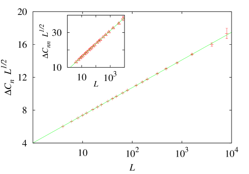
Figure 1: The quantities $\Delta C_{x}L^{1/2}=(C_{x}(\infty)-C_{x}(L))L^{1/2}$, where $x$ represents ‘n’ and ‘nn’ (inset), versus system size $L$ on a logarithmic scale. The quantities $C_{\rm n}(L)$, $C_{\rm nn}(L)$ are the amplitudes of the fluctuations in the nearest- and the next-nearest-neighbor connectivities respectively, for bond percolation on $L\times L$ square lattices with periodic boundary conditions. We use $C_{\rm n}(\infty)=4.169\;8$ and $C_{\rm nn}(\infty)=8.206$, as determined by our fits. The figures clearly indicate the presence of a logarithmic factor in the leading scaling term of $C_{\rm n}$ and $C_{\rm nn}$. The lines are added for clarity.

For the quantity $C_{\rm nn}$, which represents the amplitude of the fluctuations in $g_{\rm nn}$, a fit by $C_{\rm nn,0}+C_{\rm nn,1}L^{\psi}$ led to $C_{\rm nn,0}=8.30(3)$, $C_{\rm nn,1}=-12.8(3)$ and $\psi=-0.358(3)$, necessarily with a cutoff at a large size $L_{\rm min}=200$. These results tell that the FSS behavior of $C_{\rm nn}$ on the square lattice is similar to that of $C_{\rm n}$. A fit to the data by $C_{\rm nn,0}+d^{\prime}_{1}L^{-1/2}\ln L+d^{\prime}_{2}L^{-1/2}$ yielded $C_{\rm nn,0}=8.206(2)$, $d^{\prime}_{1}=-3.271(7)$ and $d^{\prime}_{2}=-8.43(1)$, with $L_{\rm min}=8$. Other fits with either/both of the exponents as free fitting parameters also yielded results consistent with those for $C_{\rm n}$. Thus, also the results for $C_{\rm nn}$ indicate the existence of a logarithmic factor. Data for $C_{\rm nn}$ are also presented in Table 1 and plotted in Fig. 1.

IV.2 Finite-size analysis for other lattices

IV.2.1 Triangular lattice with periodic boundary conditions

We simulated the bond-percolation problem on the triangular lattice at the percolation threshold $p^{\rm tri}_{\rm c}=2\sin(\pi/18)$ SE64 . Rhombus-shaped lattices were used, with periodic boundary conditions applied along edges of the rhombus. We used lattices with $L^{2}$ sites, with $7$ different values of the linear size $L$ in the range between $18$ and $1152$. The number of samples was $100$ million for each size. Fits of the $g_{\rm n}$ data by $g^{\rm tri}_{n,0}+c_{1}L^{y_{1}}$ yielded $g^{\rm tri}_{n,0}=0.714\;273\;9(8)$ and $y_{1}=-1.249(7)$. The value $y_{1}$ agrees well with $y_{t}-d=-5/4$. Fits of the data by Eq. (12) led to $g_{\rm n,0}^{\rm tri}=0.714\;273\;9(3)$, which is in good agreement with the theoretical prediction $0.714\;274\;133\;\cdots$ in Sec. III. For $g_{\rm nn}$, fits of the data by Eq. (12) yielded $g_{\rm nn,0}^{\rm tri}=0.637\;428\;6(5)$.

A fit of the $C_{\rm n}$ data by $C^{\rm tri}_{n,0}+c_{1}L^{\psi}$ led to $C^{\rm tri}_{n,0}=7.24(3)$, $c_{1}=-10.0(3)$ and $\psi=-0.351(8)$, with $L_{\rm min}=144$. The value $-0.351$ of the exponent is quite different from $2y_{t}-d=-1/2$. When including a logarithmic factor, a fit of the $C_{\rm n}$ data by $C^{\rm tri}_{n,0}+c_{1}L^{-1/2}+c_{2}L^{-1/2}\ln L$ yielded $C^{\rm tri}_{\rm n,0}=7.140(3)$, $c_{1}=-6.99(3)$ and $c_{2}=-2.54(2)$, with $L_{\rm min}=18$. For $C_{\rm nn}$, the first fit led to $\psi=-0.343(7)$, with $L_{\rm min}=144$, and the second fit yielded $C^{\rm tri}_{\rm nn,0}=17.595(11)$, $c_{1}=-18.5(2)$ and $c_{2}=-7.67(7)$, with $L_{\rm min}=36$.

The above results tell that the FSS behavior of the connectivities and their fluctuations on the triangular lattice is similar to that on the square lattice.

IV.2.2 Honeycomb lattice with periodic boundary conditions

We also simulated the bond-percolation problem on the honeycomb lattice at the percolation threshold $p^{\rm hon}_{\rm c}=1-2\sin(\pi/18)$. Rhombus-shaped lattices were used, with periodic boundary conditions applied along edges of the rhombus. We used lattices with $L^{2}/2$ sites, with $8$ different values of the linear size $L$ in the range between $8$ and $1024$. The number of samples was $100$ million for each size. Fits of the $g_{\rm n}$ data by $g^{\rm hon}_{n,0}+c_{1}L^{y_{1}}$ yielded $g^{\rm hon}_{n,0}=0.804\;735\;3(2)$ and $y_{1}=-1.250(1)$. The value $y_{1}$ agrees well with $y_{t}-d=-5/4$, and the numerical value of $g_{\rm n,0}^{\rm hon}$ is in good agreement with the theoretical prediction $0.804\;735\;202\;\cdots$ in Sec. III.

A fit of the $C_{\rm n}$ data by $C^{\rm hon}_{n,0}+c_{1}L^{\psi}$ led to $C^{\rm hon}_{n,0}=2.367(6)$, $c_{1}=-2.94(4)$ and $\psi=-0.351(5)$, with $L_{\rm min}=128$. The value $-0.351$ of the exponent is quite different from $2y_{t}-d=-1/2$. When including a logarithmic factor, a fit of the $C_{\rm n}$ data by $C^{\rm hon}_{n,0}+c_{1}L^{-1/2}+c_{2}L^{-1/2}\ln L$ yielded $C^{\rm hon}_{n,0}=2.332\;8(6)$, $c_{1}=-2.170(4)$ and $c_{2}=-0.722(2)$, with $L_{\rm min}=16$. Thus, as expected, the FSS behavior on the honeycomb lattice is similar to that on the square and triangular lattices. It indicates that the logarithmic factor is a universal property of two-dimensional lattices.

IV.2.3 The three-dimensional cubic lattice

The bond-percolation model on three-dimensional $L^{3}$ simple-cubic lattices with periodic boundary conditions was investigated. The simulations were done at $11$ different sizes $4\leq L\leq 256$, at a bond-occupation probability $p=p^{\rm cub}_{\rm c}=0.248\;811\;8$ WZZGD . The number of samples was over $100$ million for $L\leq 64$, and around $10$ million for $L\geq 128$.

A fit of the $g_{\rm n}$ data by $g_{\rm n,0}^{\rm cub}+c_{1}L^{y_{1}}$ led to $g_{\rm n,0}^{\rm cub}=0.359\;404\;4(3)$ and $y_{1}=-1.857\;3(14)$, with $L_{\rm min}=24$. The $y_{1}$ value is consistent with $y^{\rm(3)}_{t}-d\approx-1.859$, as it follows from the $d=3$ literature value of the thermal exponent, namely $y^{\rm(3)}_{t}=1.141\;0(15)$ WZZGD .

A fit of the $C_{\rm n}$ data by $C_{\rm n,0}^{\rm cub}+d_{1}L^{\psi}$ yielded $C_{\rm n,0}^{cub}=6.57(2)$ and $\psi=-0.602(16)$, with $L_{\rm min}=32$. Including a correction term with exponent $y^{\rm(3)}_{i}=-1.2$ WZZGD , another fit of the data by $C_{\rm n,0}^{\rm cub}+L^{\psi}(d_{1}+d_{2}L^{y^{\rm(3)}_{i}})$ led to $C_{\rm n,0}^{\rm cub}=6.57(2)$ and $\psi=-0.62(2)$, with $L_{\rm min}=16$. These values of $\psi$ are different from $2y^{\rm(3)}_{t}-d\approx-0.718$. Instead, a fit by $C_{\rm n,0}^{\rm cub}+L^{-0.718}(d_{1}+d_{2}\ln L+d_{3}L^{y^{\rm(3)}_{i}})$ led to $C_{\rm n,0}^{\rm cub}=6.556(16)$, $d_{1}=-8.0(7)$ and $d_{2}=-1.25(22)$, with $L_{\rm min}=16$. These fit results support the appearance of a multiplicative logarithmic factor in the FSS behavior of $C_{\rm n}$, which is also shown in Fig. 2.

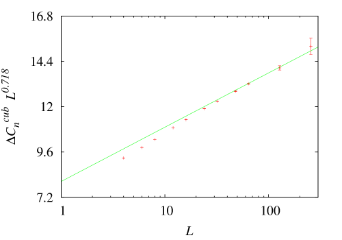
Figure 2: The quantity $\Delta C_{\rm n}^{\rm cub}L^{0.718}=(C_{\rm n}^{\rm cub}(\infty)-C_{\rm n}^{\rm cub}(L))L^{0.718}$ versus system size $L$ on a logarithmic scale. $C_{\rm n}^{\rm cub}(L)$ represents the amplitude of the fluctuations in the nearest-neighbor connectivities for percolation on a $L^{3}$ simple-cubic lattice with periodic boundary conditions. We use $C_{\rm n}^{\rm cub}(\infty)=6.566$ as obtained from the fit. The line is added for clarity. Its nonzero slope expresses the presence of a logarithmic factor in the leading finite-size dependence of $C_{\rm n}^{\rm cub}$. Deviations at small $L$ values are attributed to finite-size correction terms.

IV.2.4 The square lattice with open boundaries

We also performed bond-percolation simulations at a bond-occupation probability $p=1/2$, using a square $L\times L$ geometry, with periodic boundary conditions in one direction and open boundary conditions in the other direction. We took 11 system sizes from $L=8$ to $L=256$, and a number of $100$ million independent percolation configurations for each size, in order to sample the nearest- and next-nearest-neighbor connectivities $g_{\rm n}^{\rm sur}$ and $g_{\rm nn}^{\rm sur}$ on the open boundaries. Note that a pair of next-nearest neighbors on the boundary is separated by a distance of $2$ lattice units, instead of $\sqrt{2}$ as in the bulk.

Fits of the $g_{\rm n}^{\rm sur}$ data by $g_{\rm n,0}^{\rm sur}+c_{1}L^{y_{1}}$ yielded $g_{\rm n,0}^{\rm sur}=0.625\;000\;1(12)$ and $y_{1}=-1.999(6)$; and fits of the $g_{\rm nn}^{\rm sur}$ data led to $g_{\rm nn,0}^{\rm sur}=0.449\;789(2)$, $c_{1}=2.22(5)$ and $y_{1}=-2.005(7)$. On a free boundary, the scaling dimension of the energy operator $\epsilon$ should be replaced by $\Delta_{\epsilon}=2$ Cardy84 ($y_{\epsilon}=d-\Delta_{\epsilon}=0$). The numerical results for $g_{\rm n}^{\rm sur}$ and $g_{\rm nn}^{\rm sur}$ agree very well with $y_{1}=y_{\epsilon}-d=-\Delta_{\epsilon}$. The surface connectivities converge more quickly with the size of the system than the bulk ones, possibly because surface clusters are smaller or their correlations fall off faster, so that they are not as strongly affected by the finite size of the system.

The result for the surface connectivity strongly suggests that $g_{\rm n,0}^{\rm sur}=5/8$ holds exactly. It applies to a system with a bond probability $p=1/2$ on the open boundary. When we erase those bonds, the limiting probability that two nearest-neighboring sites on the boundary are connected decreases to $g_{\rm n,0}^{\rm sur^{\prime}}=5/32$, as can be easily checked by adding a row of $p=1/2$ bonds perpendicular to the boundary. Next, we may merge two half-infinite systems, one with, and one without boundary bonds, thus reconstructing the infinite system. The combined probability that the two nearest-neighboring sites are now connected by some path within either system is $5/8+3/8\times 5/32=175/256$, slightly smaller than the bulk value $3/4$. It thus appears that there is a probability $3/4-175/256=17/256$ that connections between the two neighboring sites exist only via paths entering both half systems.

V Origin of the logarithmic factor in the finite-size scaling

We show that the quantity $C_{\rm n}$ relates to connectivities of four points $\{\vec{x}_{1},\vec{y}_{1},\vec{x}_{2},\vec{y}_{2}\}$, in which $\vec{x}_{1}$ and $\vec{x}_{2}$ are two sites separated by a distance $r$, and $\vec{y}_{1}$, $\vec{y}_{2}$ denote a nearest neighbor of $\vec{x}_{1}$ and $\vec{x}_{2}$, respectively. In Ref. VJS, a logarithmic term was derived in the FSS of these connectivities, in the limit $q\rightarrow 1$. It was obtained from the mixing of the energy operator with the operator that connects two random clusters. These two operators become degenerate at $q=1$, with the same scaling dimension $5/4$ in two dimensions.

Following the notation of Ref. VJS, , we define $P_{0}(r)$ as the probability that the sites $\{\vec{x}_{1},\vec{y}_{1},\vec{x}_{2},\vec{y}_{2}\}$ belong to four different percolation clusters; $P_{1}(r)$ as the probability that $\{\vec{x}_{1},\vec{y}_{1},\vec{x}_{2},\vec{y}_{2}\}$ belong to three different clusters, of which one cluster connects one of $\{\vec{x}_{1},\vec{y}_{1}\}$ to one of $\{\vec{x}_{2},\vec{y}_{2}\}$; and $P_{2}(r)$ as the probability that the four points belong to two different clusters, each of which contains one point of $\{\vec{x}_{1},\vec{y}_{1}\}$ and one point of $\{\vec{x}_{2},\vec{y}_{2}\}$. The probability that the pair $\{\vec{x}_{1},\vec{y}_{1}\}$ is unconnected, while the pair $\{\vec{x}_{2},\vec{y}_{2}\}$ is simultaneously unconnected, is equal to

$$P_{0}(r)+P_{1}(r)+P_{2}(r) = \langle(1-\gamma_{x_{1}y_{1}})(1-\gamma_{x_{2}y_{2}})\rangle$$ (14)

$$= 1-2g_{\rm n}+\langle\gamma_{x_{1}y_{1}}\gamma_{x_{2}y_{2}}\rangle\;,$$

(for convenience, we omit the arrow symbol over the site coordinates here and below).
Next, we express the quantity $C_{\rm n}$ as

$$C_{\rm n} = N_{\rm e}^{-1}\left(\langle{\mathcal{E}}^{2}_{\rm n}\rangle-\langle{\mathcal{E}}_{\rm n}\rangle^{2}\right)$$ (15)

$$= N_{\rm e}^{-1}\sum_{x_{1}y_{1},\;x_{2}y_{2}}\left(\langle\gamma_{x_{1}y_{1}}\gamma_{x_{2}y_{2}}\rangle-\langle\gamma_{x_{1}y_{1}}\rangle\langle\gamma_{x_{2}y_{2}}\rangle\right)$$

$$= \left(N_{\rm e}^{-1}\sum_{x_{1}y_{1}\neq x_{2}y_{2}}\langle\gamma_{x_{1}y_{1}}\gamma_{x_{2}y_{2}}\rangle\right)+\langle\gamma_{x_{1}y_{1}}\rangle-N_{\rm e}\langle\gamma_{x_{1}y_{1}}\rangle^{2}$$

$$= \left(N_{\rm e}^{-1}\sum_{x_{1}y_{1}\neq x_{2}y_{2}}\langle\gamma_{x_{1}y_{1}}\gamma_{x_{2}y_{2}}\rangle\right)+g_{\rm n}-N_{\rm e}g_{\rm n}^{2}\;.$$

The FSS singularity of $C_{\rm n}$ resides in the first term in the last line of Eq. (15), in particular in the dependence of $\langle\gamma_{x_{1}y_{1}}\gamma_{x_{2}y_{2}}\rangle$ on the distance $r$ between $(x_{1}y_{1})$ and $(x_{2}y_{2})$. Using Eq. (14), and considering that $1-g_{\rm n}$ equals the probability that two neighboring points belong to different clusters, one derives

$$\langle\gamma_{x_{1}y_{1}}\gamma_{x_{2}y_{2}}\rangle_{r} = \left(P_{0}(r)+P_{1}(r)+P_{2}(r)-1+2g_{\rm n}\right)$$ (16)

$$= \left(P_{0}(r)+P_{1}(r)+P_{2}(r)-(1-g_{\rm n})^{2}\right)+g_{\rm n}^{2}\;.$$

According to Ref. VJS, , it behaves as $\langle\gamma_{x_{1}y_{1}}\gamma_{x_{2}y_{2}}\rangle_{r}\simeq g_{\rm n}^{2}+(a+b\ln r)r^{-2\Delta}$ in two dimensions, where $\Delta=5/4$ is the common scaling dimension of the two degenerate operators. The scaling behavior of the sum is therefore

$$N_{\rm e}^{-1}\sum_{x_{1}y_{1}\neq x_{2}y_{2}}\langle\gamma_{x_{1}y_{1}}\gamma_{x_{2}y_{2}}\rangle\approx(N_{\rm e}-1)g_{\rm n}^{2}+\int_{1}^{L/2}2\pi rdr(a+b\ln r)r^{-5/2}$$

$$=(N_{\rm e}-1)g_{\rm n}^{2}+\left(A+B\ln L\right)L^{-1/2}\;,$$ (17)

where $A$ and $B$ are non-universal constants. Substituting the above result in Eq. (15), one gets

$$C_{\rm n}(L) = C_{\rm n}(\infty)+d_{1}L^{-1/2}\ln L+d_{2}L^{-1/2}+\cdots\;.$$ (18)

This explains the multiplicative logarithmic factor in the singular part of $C_{\rm n}$.

Eq. (18) still contains a contribution due to $g_{\rm n}$, which, as noted in Sec. II.2, satisfies $g_{\rm n}=g_{n,0}+c_{1}L^{y_{t}-d}+o(L^{y_{t}-d})$. The terms in Eq. (18) originating from $g_{\rm n}$ thus contribute a constant contained in $C_{\rm n}(\infty)$, and the omitted terms include one proportional to $L^{y_{t}-d}$, etc. This conclusion is consistent with the numerical results in the previous section.

Similar arguments apply in the case of $C_{\rm nn}$. The above analysis is not restricted to the two-dimensional case. Indeed, a similar relation between $C_{\rm n}$ and the four-point connectivities holds for $d>2$; and it is expected that the energy operator and the operator which connects two random clusters become degenerate also in higher dimensions VJS ; VJ14 ; Con82 . Thus we expect a logarithmic factor also for $d>2$ in the FSS behavior of $C_{\rm n}$, which is supported by our numerical results for the three-dimensional cubic lattice in the previous section.

VI Discussion

As already clear from the work of Mitra et al. MN , critical connectivities in the percolation model display remarkable algebraic properties. Completely in line with these findings are the results for the exact eigenvectors in Appendix B, the exact value $g_{\rm n}=3/4$, and the conjectured exact values $g_{\rm nn}=11/16$ and $g_{\rm n}^{\rm sur}=5/8$ for the square-lattice model. We also derived, from the existing results for the Potts model, the exact values of $g_{\rm n}$ on the triangular and honeycomb lattices. Results from Monte Carlo simulations agree very well with these exact or conjectured values. In addition, we numerically determined some other neighboring connectivities. Our results for critical short-range connectivities in the thermodynamic limit are summarized in Tables 2 and 3. For the RC model with $q\neq 1$, the critical nearest-neighbor connectivity can be obtained from Eq. (10) and (11), for the square and triangular lattices, respectively; and for the honeycomb lattice, the nearest-neighbor connectivity can be obtained from its duality relation with that of the triangular lattice.

lattice	$g_{\rm n}$	$g_{\rm nn}$
square	$0.749\;999\;99(13)$	$0.687\;500\;0(2)$
	$3/4$	$11/16^{*}$ (Ref.MN, )
triangular	$0.714\;273\;9(3)$	$0.637\;428\;6(5)$
	$3(2+7p_{c}^{\rm tri})/4(5-p_{c}^{\rm tri})$
honeycomb	$0.804\;735\;3(2)$
	$3(-2+9p_{c}^{\rm hon})/4(1+4p_{c}^{\rm hon})$
square (surface)	$0.625\;000\;1(12)$	$0.449\;789(2)$
	$5/8^{*}$
simple cubic	$0.359\;404\;4(3)$

Table 2: Critical nearest- and next-nearest-neighbor connectivities for bond-percolation in different lattices. For each lattice, the first line shows the numerical result(s), and the second line (if applicable) presents the exact or conjectured (labeled by ‘*’) value(s). Periodic boundary conditions are used, except for the ‘square surface,’ where the connectivities are measured on free one-dimensional surfaces of the square lattice.

	$x,y$	square	$x,y$	triangular
$g_{\rm n3}$	$2,0$	$0.649\;577\;2(6)$	$2,0$	$0.619\;666\;5(6)$
$g_{\rm n4}$	$2,1$	$0.629\;978\;1(7)$	$5/2,\sqrt{3}/2$	$0.584\;475\;2(7)$
$g_{\rm n5}$	$2,2$	$0.599\;838\;6(8)$	$3,0$	$0.569\;576\;8(8)$
$g_{\rm n6}$	$3,0$	$0.595\;566\;4(8)$	$3,\sqrt{3}$	$0.552\;726\;4(8)$
$g_{\rm n7}$	$3,1$	$0.587\;653\;5(8)$	$7/2,\sqrt{3}/2$	$0.548\;185\;7(10)$
$g_{\rm n8}$	$3,2$	$0.571\;119\;2(9)$	$4,0$	$0.536\;507\;7(9)$
$g_{\rm n9}$	$4,0$	$0.560\;360\;4(12)$	$4,\sqrt{3}$	$0.526\;981\;8(10)$

Table 3: Critical third to 9th nearest-neighbor connectivities for bond-percolation in the periodic square and triangular lattices. The displacement vectors of the connectivities are listed in Cartesian coordinates under $x,y$.

In this work, for the percolation model, we also investigated the FSS behavior of the short-range connectivities and their fluctuations. As far as we know, the fluctuation amplitudes $C_{\rm n}$ and $C_{\rm nn}$ have not yet been studied before. While $g_{\rm n}$ and $g_{\rm nn}$ are energy-like quantities with leading FSS term proportional to $L^{y_{t}-d}$, so that their fluctuations may be expected to have a leading scaling exponent $2y_{t}-d$, the analysis using a simple power of the system size yields a numerical exponent that is very different from $2y_{t}-d$. This numerical exponent does not seem to fit a combination of the dimensionality and the thermal scaling dimension of the percolation problem. However, as described above, satisfactory fits (as judged from the $\chi^{2}$ criterion) are obtained by including a logarithmic factor, for $C_{\rm n}$ as well as for $C_{\rm nn}$. These results support that the fluctuations in the neighboring connectivities scale as $C-C_{0}\simeq L^{2y_{t}-d}\ln(L/L_{0})$, where $C_{0}$ is the value of the fluctuations in the thermodynamic limit, and $L_{0}$ is a non-universal factor. We have thus shown the existence of a class of observables in critical percolation with logarithmic factors in their scaling behavior, which are closely related to recently identified four-point connectivities which scale logarithmically in critical percolation VJS ; VJ14 . The origin of the logarithmic factor is different from a mechanism which introduces logarithmic factors through the $q$-dependence of the critical exponents in some critical singularities in percolation FDB . From another point of view, the observed FSS behavior may be used to determine the critical exponent $y_{t}$ in $d>2$ dimensions, where an exact value of $y_{t}$ may not be available. For example, from our results of $g_{\rm n}$ for the simple-cubic lattice, the value of $y_{t}$ for $d=3$ is obtained as $1.142\;7(14)$, which is comparable with a latest result $1.141\;0(15)$ WZZGD , and consistent with the value $8/7$ conjectured by Ziff and Stell (see LZ98 ).

Appendix A Specific-heat behavior in the limit $q\rightarrow 1$

The fluctuations in the energy-like quantities have been used to obtain specific-heat-like quantities, but thus far we have not considered the actual Potts model specific heat $C$ per site, which can be expressed as the dimensionless quantity $C/k\equiv K^{2}\partial^{2}f(K,q)/\partial^{2}K$, where $k$ is the Boltzmann constant and $f(K,q)\equiv{N_{\rm s}}^{-1}\ln Z(K,q)$ is the reduced free-energy density. While the specific heat of the random-cluster model vanishes at $q=1$, one may still ask the question how it behaves in the limit $q\to 1$. From Eq. (1) one reads that the energy change associated with the ordering of the Potts model, i.e., the integrated specific heat, is equal to $2J(q-1)/q$ for the square lattice. The $q$-dependence of the energy change, and therefore the vanishing of the specific-heat amplitude at $q=1$, can thus be compensated by introducing a normalization factor $q/(q-1)$. This is illustrated in Fig. A.1 which shows the specific heat of the random-cluster model on the square lattice, including such a factor, in the limit $q\to 1$.

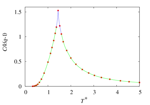
Figure A.1: (Color online). Dimensionless specific heat $C/k$ of the $q$-state Potts model on the square lattice, divided by $q-1$, versus reduced temperature $T^{*}\equiv kT/J=1/K$, in the percolation limit $q\to 1$. The Potts specific heat vanishes near $q=1$ as $q-1$, so that the normalization factor $1/(q-1)$ compensates the vanishing specific-heat amplitude. The data points (full squares) were obtained by extrapolations of finite-size data to the thermodynamic limit. Estimated error bars do not exceed the symbol sizes. The curves are added for visual aid only. The critical singularity is governed by a specific-heat exponent $\alpha=2-2/y_{t}=-2/3$. The dashed parts (blue) of the curves display the power-law behavior with this exponent. In contrast with the Ising model ($q=2$), the specific heat remains finite at the critical point; this illustrates the “nonuniversal” behaviour of the Potts model when $q$ is varied.

The quantity plotted in Fig. A.1 is equal to $K^{2}\,{\partial^{3}}f(K,q)/{\partial^{2}K}{\partial q}$ at $q=1$. The Monte Carlo calculation of this quantity is slightly more involved than that of the random-cluster specific heat QDB for general $q$, because of the additional derivative to $q$, which requires sampling of the correlation of the bond density and the cluster density at $q=1$. In particular, our numerical results were obtained by sampling of

$$\left(\frac{\partial^{3}f(K,q)}{\partial K^{2}\partial q}\right)_{q=1}=\left\{\frac{(u+1)^{2}}{u^{2}}(\langle{{\mathcal{N}}_{\rm b}}^{2}{{\mathcal{N}}_{\rm c}}/N_{\rm s}\rangle-2\langle{{\mathcal{N}}_{\rm b}}{{\mathcal{N}}_{\rm c}}/N_{\rm s}\rangle\langle{\mathcal{N}}_{\rm b}\rangle)-\frac{u+1}{u^{2}}\langle{\mathcal{N}}_{\rm b}{\mathcal{N}}_{\rm c}/N_{\rm s}\rangle\right.$$

$$\left.-\left[\frac{(u+1)^{2}}{u^{2}}(\langle{{\mathcal{N}}_{\rm b}}^{2}\rangle-2\langle{{\mathcal{N}}_{\rm b}}\rangle^{2})-\frac{u+1}{u^{2}}\langle{\mathcal{N}}_{\rm b}\rangle\right]\langle{\mathcal{N}}_{\rm c}/N_{\rm s}\rangle\right\}$$

and extrapolation to the thermodynamic limit. We simulated square systems with sizes up to $L=64$, taking numbers of samples up to a few hundred million.

The figure illustrates that the rescaled specific heat remains finite at the critical temperature, and displays a cusp-like singularity which is, as follows from the known temperature exponent NDL ; CDL of the Potts model, proportional to $|T^{*}-T^{*}_{\rm c}|^{-\alpha}$, with $\alpha=-2/3$ and the reduced temperature $T^{*}\equiv kT/J=1/K=-1/\ln(1-p)$.

Appendix B Transfer-matrix calculation of the percolation connectivities

The key observation behind the results of Ref. MN, is that the leading transfer-matrix eigenvector can be normalized such that all its components are integers. Motivated by these results, we investigated finite $L\times\infty$ bond-percolation systems with the periodic direction along a set of edges, for several values of $L$. Indeed we found that it is possible to normalize the eigenvector belonging to the largest eigenvalue such that all components are integers with greatest common divisor 1. While this eigenvector describes the connectivity at the open end of the cylinder, one can connect two of these systems by $L$ intermediate bond variables, and thus compute the connectivities on a cylinder without an open end. It is therefore possible to express the nearest- and the next-nearest-neighbor connectivities on these finite systems as exact fractions. The results of these transfer-matrix calculations are presented in Table 4. It is apparent that the connectivities converge very quickly to their infinite-system values $3/4$ and $11/16$ as $L$ increases. The data were fitted by an iterated power-law method HN82 , which yielded $g_{\rm n}=0.750\;2(8)$ and $g_{\rm nn}=0.687\;49(2)$. These fit results are consistent with the infinite-system values.

$L$	numerator	denominator	$g_{\rm n}$
$2$	$21$	$5^{2}$	$0.84$
$3$	$1201$	$39^{2}$	$0.789612097304$
$4$	$1496541$	$1393^{2}$	$0.771234389567$
$5$	$4331416849$	$75337^{2}$	$0.763156025078$
$6$	$258134675843541$	$18442085^{2}$	$0.758972970522$
$7$	$3885478927552013401$	$2266262629^{2}$	$0.756526392191$
$8$	$47703428114196051853941$	$251368505957^{2}$	$0.754966814629$
$L$	numerator	denominator	$g_{\rm nn}$
$2$	$16$	$5^{2}$	$0.64$
$3$	$114$	$13^{2}$	$0.674556213018$
$4$	$1326144$	$1393^{2}$	$0.683421208184$
$5$	$3893316098$	$75337^{2}$	$0.685966680489$
$6$	$233593856264336$	$18442085^{2}$	$0.686817539741$
$7$	$3529173407855598194$	$2266262629^{2}$	$0.687151539217$
$8$	$390852028122815173284096$	$754105517871^{2}$	$0.687302830864$

Table 4: Nearest- and next-nearest-neighbor connectivities on $L\times\infty$ square bond-percolation lattices with periodic boundary conditions along a set of edges note . They are also represented as exact fractions whose numerators and denominators are listed.

Some practical guidance is given in Ref. MN, about how one can guess a formula from a series of integer numbers. We did not succeed in guessing exact formulae for $g_{\rm n}$ and $g_{\rm nn}$ as functions of $L$. The difficulty originates from the following facts: (1) large prime numbers occur, such as $75337$ in the denominator of the fractional value of connectivities when $L=5$, and $55051$ in the factorization of $18442085$ which occurs in the denominator for $L=6$; and (2) the integers in the leading eigenvector increase very rapidly as $L$ increases. This made clear by an inspection of the smallest elements of the leading eigenvector. A list of values of these smallest elements, after normalization as mentioned above, is presented in Table 5 for several values of $L$.

$L$	2	4	6	8	10
$i$	1	$2^{2}$	$2^{6}$	$2^{12}$	$2^{20}$
$L$	3	5	7	9
$i$	3	$15\times 2^{2}$	$63\times 2^{6}$	$255\times 2^{12}$

Table 5: Integer value ($i$) of the smallest element in the normalized eigenvector which corresponds with the largest eigenvalue of the transfer-matrix for the bond-percolation problem on an $L\times\infty$ square lattice with periodic boundary conditions along a set of edges.

For even $L$, the entries in Table 5 are equal to $2^{(L-2)L/4}$ for even $L$, and for odd $L$ they are equal to $(2^{L-1}-1)2^{(L-1)(L-3)/4}$. Thus, defining $c_{L}\equiv 2^{(L-2)L/4}$, one observes that the smallest element is $c_{L}$ if $L$ is even, and $c_{L+1}-c_{L-1}$ if $L$ is odd.

Since many analytic expressions have been obtained MN for the completely packed $O(1)$ loop model, which relate to specific algebraic numbers series, such as the number of symmetric alternating sign matrices and coefficients of the characteristic polynomial of the Pascal matrix MN , one wonders if it will be possible to find exact expressions for the aforementioned connectivities as a function of $L$ in the case of the bond-percolation problem on $L\times\infty$ square lattices with the presently used periodic direction.

Appendix C Relation between percolation and $O(1)$ loop correlations

Figure C.1 illustrates the mapping of a completely packed loop configuration to a bond configuration of the corresponding bond-percolation problem BKW .

Figure C.1: Correspondence between completely packed $O(1)$ loop configurations and configurations of the bond-percolation model. The figure shows a part of a system wrapped on a cylinder, such that it is periodic in the horizontal direction and extends to infinity in both vertical directions. Solid circles show points in the middle of the lattice edges of the $O(1)$ loop model. The dual lattice of the lattice defined by these solid circles is divided into two mutually dual square sublattices, whose lattice sites are shown by open triangles and circles. Solid lines are for loops, and dashed lines are for bonds in percolation clusters on one of the dual square lattices. The dotted line indicates a row where we take the probability that two consecutive points, such as A and B, on a row lie on the same $O(1)$ loop, and the probability that two next-nearest neighbor sites, such as a and b, of the corresponding percolation configuration belong to the same cluster.

Ref. MN, gives a conjecture on the probability that $n$ consecutive points on a row lie on the same loop of the $O(1)$ loop model on $L\times\infty$ cylinders. For $n=2$, it predicts that the probability approaches $11/16$ as $L\rightarrow\infty$. We argue that, for the completely packed $O(1)$ loop model on $L\times\infty$ cylinders, the probability that two consecutive points on a row, such as A and B in Fig. C.1, lie on the same loop equals the probability that two next-nearest neighbors, such as $a$ and $b$ in Fig. C.1, are in the same percolation cluster on the corresponding square lattice. The argument is based on: (1) When two consecutive points on a row lie on the same loop, the two next-nearest neighbors on the corresponding percolation lattice belong to the same cluster. (2) When two consecutive points on a row lie on different loops, the two next-nearest neighbors on the corresponding percolation lattice belong to different clusters.

The two conclusions above can be derived as follows. In Fig. C.1, $a$ and $O$ are located on different sides of the loop through point $A$, while $b$ and $O$ are located on different sides of the loop through point $B$. In this configuration, $A$ and $B$ lie on the same loop, so that $a$ and $b$ are adjacent to and on the same side of the loop. Therefore, $a$ and $b$ belong to the same percolation cluster on the corresponding square lattice. Let us now change the loop configuration such that $A$ and $B$ lie on different loops. Then, the path $aAOBb$ crosses the loop through $A$ once, i.e., one of $a$ and $b$ belongs to the inside of that loop and the other one to the outside. Therefore, $a$ and $b$ belong to different percolation clusters.

The Mitra-Nienhuis conjecture was based on exact numerical results for systems on a cylinder with a finite circumference, which also applies to our transfer-matrix calculations for the percolation problem. However, the orientation of the $O(1)$ lattice used in Ref. MN, with respect to the axis of the cylinder differs by $\pi/4$ from our percolation lattice, so that our results for finite system do not match those for the $O(1)$ model. But these differences should vanish after extrapolation to the infinite system.

Appendix D Derivation of the exact nearest-neighbor connectivity for bond percolation on the triangular and honeycomb lattices

We first derive the exact nearest-neighbor connectivity on the triangular lattice, and then find the one on the honeycomb lattice using a duality relation. For the bond-percolation problem on the triangular lattice, with $-E_{\rm c}/3K_{\rm c}=1$ at $q=1$, from Eq. (11) one gets

$$g^{\rm tri}_{\rm n,0}=1-\left(\frac{\partial(E/3K)}{\partial q}\right)_{q=1,K=K_{\rm c}}\;.$$ (19)

The value of $K_{\rm c}$ as a function of $q$ can be obtained from Ref. KJ74, as

$$\exp{K_{\rm c}(q)}=1+\frac{\sqrt{q}}{2}\sec\left(\frac{1}{3}\arctan\sqrt{\frac{4}{q}-1}\;\right)\;,$$ (20)

and the reduced internal energy at $K=K_{\rm c}$ is given in Ref. BTA78, as

$$E_{\rm c}(q)=-3\epsilon\csc(2\phi)\sin(2\phi/3)\sin(4\phi/3)\int^{\infty}_{-\infty}\frac{\sinh[(\pi-\phi)x]\cosh(2\phi x/3)}{\sinh(\pi x)\cosh(\phi x)}{\rm d}x\;,$$ (21)

with $\cos\phi={\sqrt{q}}/{2}\;\;\;\;(0<\phi<\frac{\pi}{2})$, $\epsilon=\ln[2\cos(2\phi/3)]$, and $q<4$.

Substituting $K_{\rm c}(q)$ and $E_{\rm c}(q)$ into Eq. (19), we derive the exact connectivity in the limit $q\rightarrow 1$ as

$$g_{\rm n,0}^{\rm tri} = 1-\frac{8\ln\left(2\cos{\frac{2\pi}{9}}\right)\sin^{2}{\frac{\pi}{9}}\left(3\sqrt{3}-\tan{\frac{\pi}{9}}\right)\cos{\frac{\pi}{18}}}{9\ln^{2}\left[\frac{1}{2}\left(2+\sec{\frac{\pi}{9}}\right)\right]\left(2+\sec{\frac{\pi}{9}}\right)}$$ (22)

$$+\frac{12\cos{\frac{\pi}{9}}-8\cos{\frac{2\pi}{9}}-4\sin{\frac{\pi}{18}}-2\ln\left(2\cos{\frac{2\pi}{9}}\right)\left(7+4\sin{\frac{\pi}{18}}\right)}{9\ln\left[\frac{1}{2}\left(2+\sec{\frac{\pi}{9}}\right)\right]\left(2+\sec{\frac{\pi}{9}}\right)}$$

$$+\frac{{\ln\left(2\cos\frac{2\pi}{9}\right)}{\cos\frac{\pi}{18}}\left\{-{8\cot\frac{\pi}{9}}+{3\csc\frac{2\pi}{9}}+\left[-21+16\sqrt{13}{\cos\left(\frac{1}{3}\arctan{\frac{53\sqrt{3}}{19}}\right)}\right]{\sin\frac{2\pi}{9}}\right\}}{9\ln\left[\frac{1}{2}\left(2+\sec{\frac{\pi}{9}}\right)\right]}$$

$$= \frac{3(2+7p_{c}^{\rm tri})}{4(5-p_{c}^{\rm tri})}=\frac{3(2+14\sin[\pi/18])}{4(5-2\sin[\pi/18])}=0.714\;274\;133\;\cdots\;,$$

where $p_{c}^{\rm tri}=2\sin(\pi/18)$ is the bond-percolation threshold on the triangular lattice SE64 . The derivation involved the calculation of several complicated integrals, which led to an intermediate result (the first three lines of Eq. (22)). We found the simplified expression in the last line of Eq. (22) with the help of an answer engine WA using numerical values of the intermediate result. We verified that the two results are exactly equal. In the verification, we made use of the identities $4\cos(2\pi/9)=2+\sec(\pi/9)$ and $\sqrt{13}\cos(\arctan[{53\sqrt{3}}/{19}]/3)=(4+7\sin[\pi/18])/(3-8\sin[\pi/18])$.

From the above $g_{\rm n,0}^{\rm tri}$, one obtains the value of $g_{\rm n,0}^{\rm hon}$ as follows. Let $p^{\rm tri}_{\rm c}$ be the critical bond-occupation probability on the triangular lattice, and $p^{\rm tri}_{\rm o}$ the probability that two nearest-neighbor sites are connected via some path of bonds not covering the bond between the two sites. Then, $(1-p^{\rm tri}_{\rm c})p^{\rm tri}_{\rm o}$ is the probability that there is no bond between nearest-neighbor sites, while the sites are still connected. Thus

$$g_{\rm n}^{\rm tri}=p^{\rm tri}_{\rm c}+(1-p^{\rm tri}_{\rm c})p^{\rm tri}_{\rm o}\;.$$ (23)

Similarly, one can write for the honeycomb lattice

$$g_{\rm n}^{\rm hon}=p^{\rm hon}_{\rm c}+(1-p^{\rm hon}_{\rm c})p^{\rm hon}_{\rm o}\;.$$ (24)

The duality property tells that

$$p^{\rm tri}_{\rm c}+p^{\rm hon}_{\rm c}=1\;,\;\;\;\;p^{\rm tri}_{\rm o}+p^{\rm hon}_{\rm o}=1\;.$$ (25)

The substitution of Eqs. (25) and (23) into Eq. (24) yields

$$g_{\rm n}^{\rm hon}=1-p_{c}^{\rm tri}+p_{c}^{\rm tri}\left(1-\frac{g_{\rm n}^{\rm tri}-p_{c}^{\rm tri}}{1-p_{c}^{\rm tri}}\right)$$ (26)

Using the above equation and the $g_{\rm n,0}^{\rm tri}$ value as given in Eq. (22), one obtains

$$g_{\rm n,0}^{\rm hon} = \frac{3(7-9p_{c}^{\rm tri})}{4(5-4p_{c}^{\rm tri})}=\frac{3(-2+9p_{c}^{\rm hon})}{4(1+4p_{c}^{\rm hon})}=\frac{3(-7+18\sin[\pi/18])}{4(-5+8\sin[\pi/18])}$$ (27)

$$= 0.804\;735\;202\;\cdots.$$

References

- (1) D. Stauffer and A. Aharony, Introduction to Percolation Theory (Taylor & Francis, London, 1992), revised 2nd ed.
- (2) P. Kleban, J. J. H. Simmons and R. M. Ziff, Phys. Rev. Lett. 97, 115702 (2006); J. J. H. Simmons, P. Kleban and R. M. Ziff, Phys. Rev. E 76, 041106 (2007); G. Delfino and J. Viti, J. Phys. A: Math. Theor. 44 032001 (2011); R. M. Ziff, J. J. H. Simmons and P. Kleban, J. Phys. A: Math. Theor. 44 065002 (2011); and references therein.
- (3) R. Vasseur, J. L. Jacobsen and H. Saleur, J. Stat. Mech. L07001 (2012).
- (4) R. Vasseur and J. L. Jacobsen, Nucl. Phys. B 880, 435 (2014).
- (5) R. B. Potts, Proc. Cambridge Philos. Soc. 48, 106 (1952).
- (6) F. Y. Wu, J. Stat. Phys. 18, 115 (1978).
- (7) P. W. Kasteleyn and C. M. Fortuin, J. Phys. Soc. Jpn. 26 (Suppl.), 11 (1969); C. M. Fortuin and P. W. Kasteleyn, Physica (Utrecht) 57, 536 (1972).
- (8) R. M. Ziff, S. R. Finch and V. S. Adamchik, Phys. Rev. Lett 79, 3447 (1997).
- (9) H. Hu, H. W. J. Blöte, Y. Deng, J. Phys. A: Math. Theor. 45 494006 (2012).
- (10) D. Kim and R. I. Joseph, J. Phys. C: Solid State Phys., 7, L167 (1974).
- (11) R. J. Baxter, H. N. V. Temperley and S. E. Ashley, Proc. R. Soc. Lond. A 358 535 (1978).
- (12) S. Mitra, B. Nienhuis, J. de Gier and M. T. Batchelor, J. Stat. Mech. P09010 (2004); S. Mitra and B. Nienhuis, ibid. P10006 (2004); B. Nienhuis, private communication.
- (13) B. Nienhuis, in Phase Transitions and Critical Phenomena, edited by C. Domb and J. L. Lebowitz (Academic, London, 1987), Vol. 11, p. 1.
- (14) J. L. Cardy, in Phase Transitions and Critical Phenomena, edited by C. Domb and J. L. Lebowitz (Academic, London, 1987), Vol. 11, p. 55.
- (15) J. Wang, Z. Zhou, W. Zhang, T. M. Garoni and Y. Deng, Phys. Rev. E 87, 052107 (2013).
- (16) A. Coniglio, Phys. Rev. Lett. 62, 3054 (1989).
- (17) M. F. Sykes and J. W. Essam, J. Math. Phys. 5, 1117 (1964).
- (18) J. L. Cardy, Nucl. Phys. B 240, 514 (1984).
- (19) A. Coniglio, J. Phys. A: Math. Gen. 15, 3829 (1982).
- (20) X. Feng, Y. Deng and H. W. J. Blöte, Phys. Rev. E 78, 031136 (2008).
- (21) C. D. Lorenz and R. M. Ziff, Phys. Rev. E 57, 230 (1998).
- (22) X. Qian, Y. Deng and H. W. J. Blöte, Phys. Rev. E 71, 016709 (2005).
- (23) H. W. J. Blöte and M. P. Nightingale, Physica A 112, 405 (1982).
- (24) R. J. Baxter, S. B. Kelland and F. Y. Wu, J. Phys. A 9, 397 (1976).
- (25) WolframAlpha (http://www.wolframalpha.com).
- (26) The values presented in this table was calculated in the vertical direction of the cylinder (the direction which extends to infinity). We also conducted an exact enumeration for in the horizontal direction with . These results tells that the average of in the two directions is exactly for . By using a self-dual property of the square lattice, it can be exactly proved that the average of in the two directions is for .