Improved Graph Laplacian via Geometric Self-Consistency

Abstract

We address the problem of setting the kernel bandwidth $\epsilon$ used by Manifold Learning algorithms to construct the graph Laplacian. Exploiting the connection between manifold geometry, represented by the Riemannian metric, and the Laplace-Beltrami operator, we set $\epsilon$ by optimizing the Laplacian’s ability to preserve the geometry of the data. Experiments show that this principled approach is effective and robust.

1 Introduction

Manifold learning and manifold regularization are popular tools for dimensionality reduction and clustering Belkin and Niyogi (2002); von Luxburg et al. (2008), as well as for semi-supervised learning Belkin et al. (2006); Zhu et al. (2003); Zhou and Belkin (2011); Smola and Kondor (2003) and modeling with Gaussian Processes Sindhwani et al. (2007). Whatever the task, a manifold learning method requires the user to provide an external parameter, called “bandwidth” or “scale” $\epsilon$, that defines the size of the local neighborhood.

More formally put, a common challenge in semi-supervised and unsupervised manifold learning lies in obtaining a “good” graph Laplacian estimator $L$. We focus on the practical problem of optimizing the parameters used to construct $L$ and, in particular, $\epsilon$. As we see empirically, since the Laplace-Beltrami operator on a manifold is intimately related to the geometry of the manifold, our estimator for $\epsilon$ has advantages even in methods that do not explicitly depend on $L$.

In manifold learning, there has been sustained interest for determining the asymptotic properties of $L$ Giné and Koltchinskii (2006); Belkin and Niyogi (2007); Hein et al. (2007); Ting et al. (2010). The most relevant is Singer (2006), which derives the optimal rate for $\epsilon$ w.r.t. the sample size $N$

$$\epsilon^{2}=C(\mathcal{M})N^{-\frac{1}{3+d/2}}\\ ,$$ (1)

with $d$ denoting the intrinsic dimension of the data manifold $\mathcal{M}$. The problem is that $C(\mathcal{M})$ is a constant that depends on the yet unknown data manifold, so it is rarely known in practice. Also, this result is asymptotic, in the limit of very large sample sizes.

Considerably fewer studies have focused on the parameters used to construct $L$ in a finite sample problem. A common approach is to “tune” parameters by cross-validation in the semi-supervised context. However, in an unsurpervised problem like non-linear dimensionality reduction, there is no context in which to apply cross-validation. While several approaches Lee and Verleysen (2007); Chen and Buja (2009); Levina and Bickel (2005); Carter et al. (2007) may yield a usable parameter, they generally do not aim to improve $L$ per se and offer no geometry-based justification for its selection.

In this paper, we present a new, geometrically inspired approach to selecting the bandwidth parameter $\epsilon$ of $L$ for a given data set. It is known that, in the hypothesis that the data come from a manifold $\mathcal{M}$, the Laplace-Beltrami operator $\Delta_{\mathcal{M}}$ on the data manifold $\mathcal{M}$ contains all the intrinsic geometry of $\mathcal{M}$. Hence, we compare the geometry induced by the graph Laplacian $L$ with the local data geometry and choose the value of $\epsilon$ for which these two are closest.

2 Background: Heat Kernel, Laplacian and Geometry

Our paper builds on two previous sets of results: 1) the construction of $L$ that is consistent for $\Delta_{\mathcal{M}}$ when the sample size $N\rightarrow\infty$ under the manifold hypothesis (see Coifman and Lafon (2006)); and 2) the relationship between $\Delta_{\mathcal{M}}$ and the Riemannian metric $g$ on a manifold, as well as the estimation of $g$ (see Perraul-Joncas and Meila (2013)).

Construction of the graph Laplacian. Several methods could be used to construct $L$ (see Hein et al. (2007); Ting et al. (2010)). The one we present, due to Coifman and Lafon (2006), guarantees that, if the data are sampled from a manifold $\mathcal{M}$, $L$ converges to $\Delta_{\mathcal{M}}$:

Given a set of points $\mathcal{D}=\{x_{1},\dots,x_{N}\}$ in high-dimensional Euclidean space $\mathbb{R}^{r}$, construct a weighted graph ${\cal G}=(\mathcal{D},W)$ over them, with $W=[W_{ij}]_{ij=1:N}$. The weight $W_{ij}$ between $x_{i}$ and $x_{j}$ is the heat kernel Belkin and Niyogi (2002)

$$W_{ij}\,\equiv\,W_{\epsilon}(x_{i},x_{j})\,=\,\exp\left(\left|\left|x_{i}-x_{j}\right|\right|_{2}^{2}/\epsilon^{2}\right),$$ (2)

with $\epsilon$ a bandwidth parameter fixed by the user. Next, construct $L=[L_{ij}]_{ij}$ of ${\cal G}$ by

$$\!\!\!\!d_{i} \!\!\!\!\!\!= \!\!\!\!\!\!\sum_{j}W_{ij}\,,\;\;\;W^{\prime}_{ij}=\frac{W_{ij}}{d_{i}d_{j}}\,,\;\;\;d^{\prime}_{i}=\sum_{j}W^{\prime}_{ij}\,,\;\text{and}\,\,L_{ij}=\sum_{j}\frac{W^{\prime}_{ij}}{d^{\prime}_{j}}\,.$$ (3)

Equation (3) represents the discrete versions of the renormalized Laplacian construction from Coifman and Lafon (2006). Note that $d_{i},d^{\prime}_{i},W^{\prime},L$ all depend on the bandwidth $\epsilon$ via the heat kernel.

Estimation of the Riemannian metric. We follow Perraul-Joncas and Meila (2013) in this step. A Riemannian manifold $(\mathcal{M},g)$ is a smooth manifold $\mathcal{M}$ endowed with a Riemannian metric $g$; the metric $g$ at point $p\in\mathcal{M}$ is a scalar product over the vectors in $\mathcal{T}_{p}\mathcal{M}$, the tangent subspace of $\mathcal{M}$ in $p$. In any coordinate representation of $\mathcal{M}$, $g_{p}\equiv G(p)$ – the Riemannian metric at $p$ – represents a positive definite matrix of dimension $d$ equal to the intrinsic dimension of $\mathcal{M}$. The significance of the metric $g$ as a repository of the geometry of $\mathcal{M}$ arises mainly from two facts: (i) the volume element for any integration over $\mathcal{M}$ is given by $\sqrt{\det G(x)}dx$, and (ii) the line element for computing distances along a curve $x(t)\subset\mathcal{M}$ is $\sqrt{\left(\frac{dx}{dt}\!\right)\!^{T}\!G(x)\frac{dx}{dt}}$.

If we assume that the data we observe (in $\mathbb{R}^{r}$) lies on a manifold, then in the original coordinates, the metric $G(p)$ is the unit matrix of dimension $d$ padded with zeros up to dimension $r$. When the data is mapped to another coordinate system – for instance by a manifold learning algorithm that performs non-linear dimension reduction – the matrix $G(p)$ changes with the coordinates to reflect the distortion induced by the mapping (see Perraul-Joncas and Meila (2013) for more details).

Proposition 1

Let $x$ denote local coordinate functions of a smooth Riemannian manifold $(\mathcal{M},g)$ of dimension $d$ and $\Delta_{\mathcal{M}}$ the Laplace-Beltrami operator defined on $\mathcal{M}$. Then:
1.Rosenberg (1997) For any function $f\in{\cal C}^{2}(\mathcal{M})$

$$\Delta_{\mathcal{M}}f\;=\;\frac{1}{\sqrt{\text{det}(G)}}\sum_{l=1}^{d}\frac{\partial}{\partial x^{l}}\left(\sqrt{\text{det}(G)}\sum_{k=1}^{d}(G^{-1})_{lk}\frac{\partial}{\partial x^{k}}f\right).$$

2. $H(p)=(G(p))^{-1}$ the (matrix) inverse of the Riemannian metric at point $p$, is given by

$$(H(p))^{ij}\;=\;\frac{1}{2}\Delta_{\mathcal{M}}\left(x^{i}-x^{i}(p)\right)\left(x^{j}-x^{j}(p)\right)|_{x=x(p)}$$ (4)

with $i,j=1,\dots,d$

In (4) above, the right hand side is the application of the $\Delta_{\mathcal{M}}$ operator to the function $\left(x^{i}-x^{i}(p)\right)\left(x^{j}-x^{j}(p)\right)$, where $x^{i},x^{j}$ denote coordinates $i,j$ seen as functions on $\mathcal{M}$ and $x(p)$ is the coordinate map evaluated at point $p\in\mathcal{M}$. The inverse matrices $(g_{p})^{-1}=h_{p}\equiv H(p)$, being symmetric and positive definite, determine a Riemannian metric $h$ called the dual metric on $\mathcal{M}$.

Proposition 1 shows that the geometry of a smooth manifold $\mathcal{M}$ is completely encoded by $\Delta_{\mathcal{M}}$ and, conversely, that $g$ completely determines $\Delta_{\mathcal{M}}$. Through (4), it also provides a way to estimate $g$ from data. Algorithm 1, adapted from Perraul-Joncas and Meila (2013), implements (4).

Algorithm 1 Riemannian Metric($X,i,L,dual\in\{-1,1\}$)

  Input: $N\times d$ design matrix $X$, $i$ index in data set, Laplacian $L$, binary variable $dual$

  for $k=1\to d$, $l=1\to d$ do

     $H_{k,l}\leftarrow\sum_{j=1}^{N}L_{ij}\left(X_{jk}-X_{ik})(X_{jl}-X_{il}\right)$

  end for

  return  $H^{dual}$ (i.e. $H$ if $dual=1$ and $H^{-1}$ if $dual=-1$)

3 A Quality Measure for $L$

Having established that the Laplace-Beltrami operator on a manifold $\mathcal{M}$ encodes the intrinsic geometry of $\mathcal{M}$, we propose to estimate $\epsilon$ by optimizing how faithfully the corresponding $L$ captures the original data geometry. For this we must: (1) estimate the geometry $g$ both from $L$ and without $L$ (Section 3.2), and (2) define a measure of agreement between the two (Section 3.3).

3.1 The Geometric Consistency Idea for Optimizing $L$

We consider the trivial embedding of the data in the ambient space $\mathbb{R}^{r}$ for which the geometry is trivially known. This provides a target $g$; we tune the scale of the Laplacian so that the $g$ calculated from Proposition 1 matches this target. Hence, we choose $\epsilon$ to maximize self-consistency in the geometry of the data.

More precisely, if $\mathcal{M}\subset\mathbb{R}^{r}$ and inherits its metric from $\mathbb{R}^{r}$, as per the generally assumed hypothesis for dimensionality reduction, then the Riemannian metric of $\mathcal{M}$ is $g_{\mbox{\raisebox{-0.60275pt}{\tiny$\!\mathbb{R}^{r}$}}}|_{T\mathcal{M}}$. Here, $g_{\mbox{\raisebox{-0.60275pt}{\tiny$\!\mathbb{R}^{r}$}}}|_{T\mathcal{M}}$ stands for the restriction of the natural metric of the ambient space $\mathbb{R}^{r}$ to the tangent bundle $T\mathcal{M}$ of the manifold $\mathcal{M}$. We propose to tune the parameters of the graph Laplacian $L$ so as to approximately enforce (a discrete, coordinate expression of) the identity

$$g_{p}\equiv g_{\mbox{\raisebox{-0.60275pt}{\tiny$\!\mathbb{R}^{r}$}}}|_{T_{p}\mathcal{M}}\,\forall p\in\mathcal{M}\,.$$ (5)

In the above, the l.h.s. will be the metric implied from the Laplacian via Proposition 1, and the r.h.s will be described below. Mathematically speaking, (5) is necessary and sufficient for finding the “correct” Laplacian.

Note also that the geometric self-consistency approach is not limited to the bandwidth parameter $\epsilon$, but can be applied to any other parameter used in the construction of the Laplacian.

3.2 Robust Estimation of the Metric

Exploiting equivalence (5) to optimize the graph Laplacian involves estimating $g$ from $L$ as prescribed by Proposition 1 and representing the r.h.s $g_{\mbox{\raisebox{-0.60275pt}{\tiny$\!\mathbb{R}^{r}$}}}|_{T_{p}\mathcal{M}}$numerically. Doing the latter directly via equation (4) is possilble, but naive, since it will yield a $r\times r$ matrix of rank $d$. Computing such a large matrix is both inefficient and sensitive to noise in the data.

Instead, we estimate the tangent bundle $T\mathcal{M}$ and reduce the required computations for (4) from $Nr^{2}$ to $Nd^{2}$ by performing them directly on $T\mathcal{M}$. Specifically, we evaluate the tangent subspace around each sampled point $x_{i}$ using local Principal Component Analysis (PCA) and then express $g_{\mbox{\raisebox{-0.60275pt}{\tiny$\!\mathbb{R}^{r}$}}}|_{T_{p}\mathcal{M}}$ directly in the resulting low-dimensional subspace as the unit matrix $I_{d}$. The tangent subspace also serves to define a local coordinate chart, which is passed as input to Algorithm 1, which computes $g_{p}$ in these coordinates.

When we compute $T_{x_{i}}\mathcal{M}$, for the sake of consistency, and to ensure that the geometry we encode is common to all the transformations we perform, we equate the notion of neighborhood in the local PCA with that embodied in the heat kernel by choosing the same bandwidth $\epsilon$ in both. This means that we conduct a weighted local PCA (wlPCA), with weights defined by the heat kernel used to produce the graph Laplacian (2), centered around $x_{i}$. This approach is similar to sample-wise weighted PCA of Yue et al. (2004), with two important requirements: the weights must decay rapidly away from $x_{i}$, and the data must be centered to have zero mean such that all the points far from $x_{i}$ are mapped close to the origin. These are satisfied by the weighted recentered design matrix $Z$, where $Z_{j:}$, row $j$ of $Z$, is given by:

$$Z_{j:}\,=\,\frac{W_{ij}(x_{j}-\bar{x})}{\sum_{j^{\prime}=1}^{N}W_{ij^{\prime}}}\,,\,\,\,\text{with}\;\bar{x}\,=\,\sum_{j=1}^{N}\frac{W_{ij}x_{j}}{\sum_{j^{\prime}=1}^{N}W_{ij^{\prime}}}\,.$$ (6)

Aswani et al. (2011) proves that the wlPCA using the heat kernel, and equating the PCA and heat kernel neighborhoods as we do, yields a consistent estimator of $T_{x_{i}}\mathcal{M}$. This is implemented in Algorithm 2.

Algorithm 2 Tangent Plane Projection($X,w,d$)

  Input: $N\times r$ design matrix $X$, weight vector $w=[W_{i1}\,\ldots\,W_{iN}]$, dimension $d$

  Compute $Z,\,\bar{x}$ using (6)

  $[V,\Lambda]\leftarrow\text{eig}(Z^{t}Z,d)$ ($d$-SVD of $Z$)

  Center $X$ around $\bar{x}$ from (6)

  $Y\leftarrow XV_{:,1:d}$ (Project $X$ on $d$ principal subspace)

  return  Y

In summary, to estimate the Riemannian metric at a point $x_{i}\in\mathcal{D}$, one must (i) construct the graph Laplacian by (3); (ii) perform Algorithm 2 to obtain $Y$; and (iii) apply Algorithm 1 to $Y$ to obtain $G(x_{i})\in\mathbb{R}^{d\times d}$. This matrix is then compared with $I_{d}$.

We now take this approach a few steps further in terms of improving its robustness with minimal sacrifice to its theoretical grounding. First, it is debatable whether inverting $H$ in Algorithm 1 is necessary. Relation (5) is trivially satisfied for the inverse Riemannian metric $g_{\mbox{\raisebox{-0.60275pt}{\tiny$\!\mathbb{R}^{r}$}}}^{-1}$ since in the chosen coordinates both $g_{\mbox{\raisebox{-0.60275pt}{\tiny$\!\mathbb{R}^{r}$}}}$ and $g_{\mbox{\raisebox{-0.60275pt}{\tiny$\!\mathbb{R}^{r}$}}}^{-1}$ are equal to the unit matrix $I_{d}$. Therefore we will use the dual metric $h$ in place of $g$ by default. Second, we perform both Algorithm 2 and Algorithm 1 in $d^{\prime}$ dimensions, with $d^{\prime}\leq d$.

These changes make the algorithm faster, and make the computed dual metric $H$ both more stable numerically and more robust to possible noise in the data. Proposition 2 shows that the resulting method remains theoretically sound.

Proposition 2

Let $X,\,Y,\,Z,\,V,\,W_{:i},\,H$, and $d\geq 1$ represent the quantities in Algorithms 1 and 2; assume that the columns of $V$ are sorted in decreasing order of the singular values, and that the rows and columns of $H$ are sorted according to the same order. Now denote by $Y^{\prime},\,V^{\prime},\,H^{\prime}$ the quantitities computed by Algorithms 1 and 2 for the same $X,\,W_{:i}$ but with $d\leftarrow d^{\prime}=1$. Then,

$$V^{\prime}\,=\,V_{:1}\in\mathbb{R}^{r\times 1}\;\;Y^{\prime}\,=\,Y_{:1}\in\mathbb{R}^{N\times 1}\;\;H^{\prime}\,=\,H_{11}\in\mathbb{R}.$$ (7)

The proof of this result is straightforward and omitted for brevity. It is easy to see that Proposition 2 generalizes immediately to any $1\leq d^{\prime}<d$. In other words, by using $d^{\prime}<d$, we will be projecting the data on a proper subspace of $T_{x_{i}}\mathcal{M}$ – namely, the subspace of least curvature Lee (1997). The dual metric $H^{\prime}$ of this projection is the principal submatrix of order $d^{\prime}$ of $H$, i.e. $H_{11}$ if $d^{\prime}=1$. Therefore, with the reduced rank algorithms, we will only be enforcing a submatrix of $H$ to be close to the unit matrix.

3.3 Measuring the Distortion

For a finite sample, we cannot expect (5) to hold exactly, and so we need to define a distortion between the two metrics to evaluate how well they agree. We propose the distortion

$${D}\;=\;\frac{1}{N}\sum_{i=1}^{N}||H(x_{i})-I_{d}||$$ (8)

where $||A||=\lambda_{max}(A)$ is the matrix spectral norm. Thus ${D}$ measures the average distance of $H$ from the unit matrix over the data set. For a “good” Laplacian, the distortion ${D}$ should be minimal:

$$\hat{\epsilon}\;=\;\text{argmin}_{\epsilon}{D}\,.$$ (9)

Before moving on, we note that the spectral norm in (8) is not chosed arbitrarily. The expression of ${D}$ in (8) is the discrete version of the distance function $D_{g_{0}}$ on the space of Riemannian metrics of a manifold $\mathcal{M}$ defined by

$${D}_{g_{0}}\left(g_{1},g_{2}\right)\,=\,\int_{\mathcal{M}}\left|\left|g_{1}-g_{2}\right|\right|_{g_{0}}dV_{g_{0}},$$ (10)

with volume element $dV_{g_{0}}=\sqrt{\text{det}G_{0}(x)}dx$ and

$$\bigl{.}\left|\left|g\right|\right|_{g_{0}}\bigr{|}_{p}\;=\;\sup_{u,v\in\mathcal{T}_{p}\mathcal{M}\setminus\{0\}}\frac{<u,v>_{g_{p}}}{<u,v>_{g_{0p}}}.$$ (11)

Furthermore, the right-hand side of (11) above represents the tensor norm of $g_{p}$ on $\mathcal{T}_{p}\mathcal{M}$ with respect to the Riemannian metric $g_{0p}$. Now, (8) follows when $g_{0},g_{1},g_{2}$ are replaced by $I,\,I$ and $H$, respectively.

With (9), we have established a principled criterion for selecting the parameter(s) of the graph Laplacian, by minimizing the distortion between the true geometry and the geometry derived from Proposition 1. Practically, we compute ${D}$ by Algorithm 3 for each candidate $\epsilon$ , then choose $\hat{\epsilon}$ by (9).

Algorithm 3 Compute Distortion$(X,\epsilon,d)$

  Input: $N\times r$ design matrix $X$, $\epsilon$, working dimension $d$

  Compute the heat kernel $W$ by (2) for each pair of points in $X$

  Compute the graph Laplacian $L$ from $W$ by (3)

  ${D}\leftarrow 0$

  for $i=1\to n$ do

     $Y\leftarrow$ TangentPlaneProjection($X,W_{i,:},d$)

     $H\leftarrow$ RiemannianMetric($Y,L,dual=1$)

     ${D}\leftarrow{D}+||H-I_{d}||^{2}/N$

  end for

  return  ${D}$

4 Related Work

Although the problem of estimating the “scale” of the data is pervasive in manifold learning, work has focused mainly on asymptotic results, with very few papers proposing estimation methods that can be implemented in practice.

We have already mentioned the asymptotic result (1) of Singer (2006). Other work in this area (Giné and Koltchinskii (2006); Hein et al. (2007); Ting et al. (2010)) provides the necessary rates of change for $\epsilon$ with respect to $N$ to guarantee convergence. These studies are relevant; however, they all depend on manifold parameters that are usually not known.

Among practical methods, the most interesting is that of Chen and Buja (2009), which estimates $k$, the number of nearest neighbors to use in the construction of the graph Laplacian. It is reminiscent of our method, in that it is self-consistent and evaluates a given $k$ with respect to the preservation of $k^{\prime}$ neighborhoods in the original data. However, it is not known how a method for estimating $k$ can be translated into a method for estimating $\epsilon$ or vice versa (the two graph construction methods exhibit different asymptotic behaviour precisely because they give rise to different ensembles of neighborhoods Ting et al. (2010)).

Moreover, the method of Chen and Buja (2009) is designed to optimize for a specific embedding, so the values obtained for $k$ depend on the embedding algorithm used. By contrast, the selection algorithm we propose estimates an intrinsic quantity, a scale $\epsilon$ that depends exclusively on the data. It is known Goldberg et al. (2008) that most embeddings induce distortion in the data geometry. Therefore, it is not clear that minimizing reconstruction error for a particular method - Laplacian Eigenmap, for example - is optimal, since even in the limit of infinite data, the embedding will distort the original geometry.

Finally, we mention the algorithm proposed in Chen et al. (2011) (CLMR). Its goal is to obtain an estimate of the intrinsic dimension of the data; however, a by-product of the algorithm is a range of scales where the tangent space at a data point is well aligned with the principal subspace obtained by a local singular value decomposition. As these are scales at which the manifold looks locally linear, one can reasonably expect that they are also the correct scales at which to approximate differential operators, such as $\Delta_{\mathcal{M}}$. Given this, we implement the method and compare it to our own results.

5 Experimental Results

Synthethic Data. We experimented with estimating the bandwidth $\hat{\epsilon}$ on data sampled from known manifolds with noise. We considered the two-dimensional hourglass and dome manifolds of Figure 1. We sampled uniformly from these manifolds, adding 10 “noise” dimensions and Gaussian noise ${\cal N}(0,\sigma^{2})$ to the resulting 13 dimensions.

The range of $\epsilon$ values was delimited by $\epsilon_{min}$ and $\epsilon_{max}$. We set $\epsilon_{max}$ to the average of $||x_{i}-x_{j}||^{2}$ over all point pairs and $\epsilon_{min}$ to the limit in which the heat kernel $W$ becomes approximately equal to the unit matrix; this is tested by $\max_{j}(\sum_{i}W_{ij})-1<\gamma$ for $\gamma\approx 10^{-4}$. This range spans about two orders of magnitude in the data we considered, and was searched by a logarithmic grid with approximately 20 points. We saved computatation time by evaluating all pointwise quantities ($\hat{{D}}$, local SVD) on a random sample of size $N^{\prime}=200$ of each data set. We replicated each experiment on 10 independent samples.

	${\mathsf{\sigma}=0.001}$	${\mathsf{\sigma}=0.01}$	${\mathsf{\sigma}=0.1}$

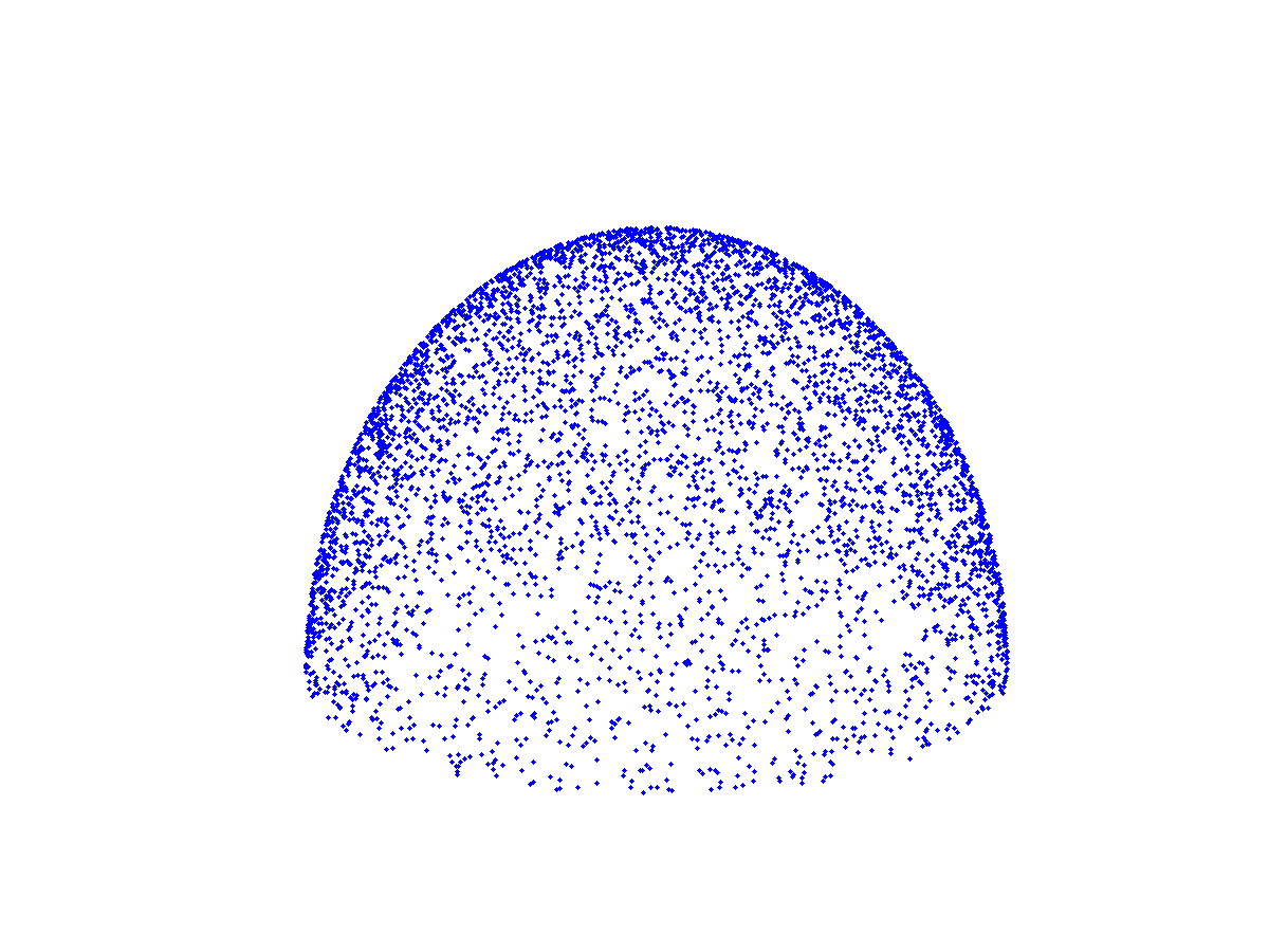
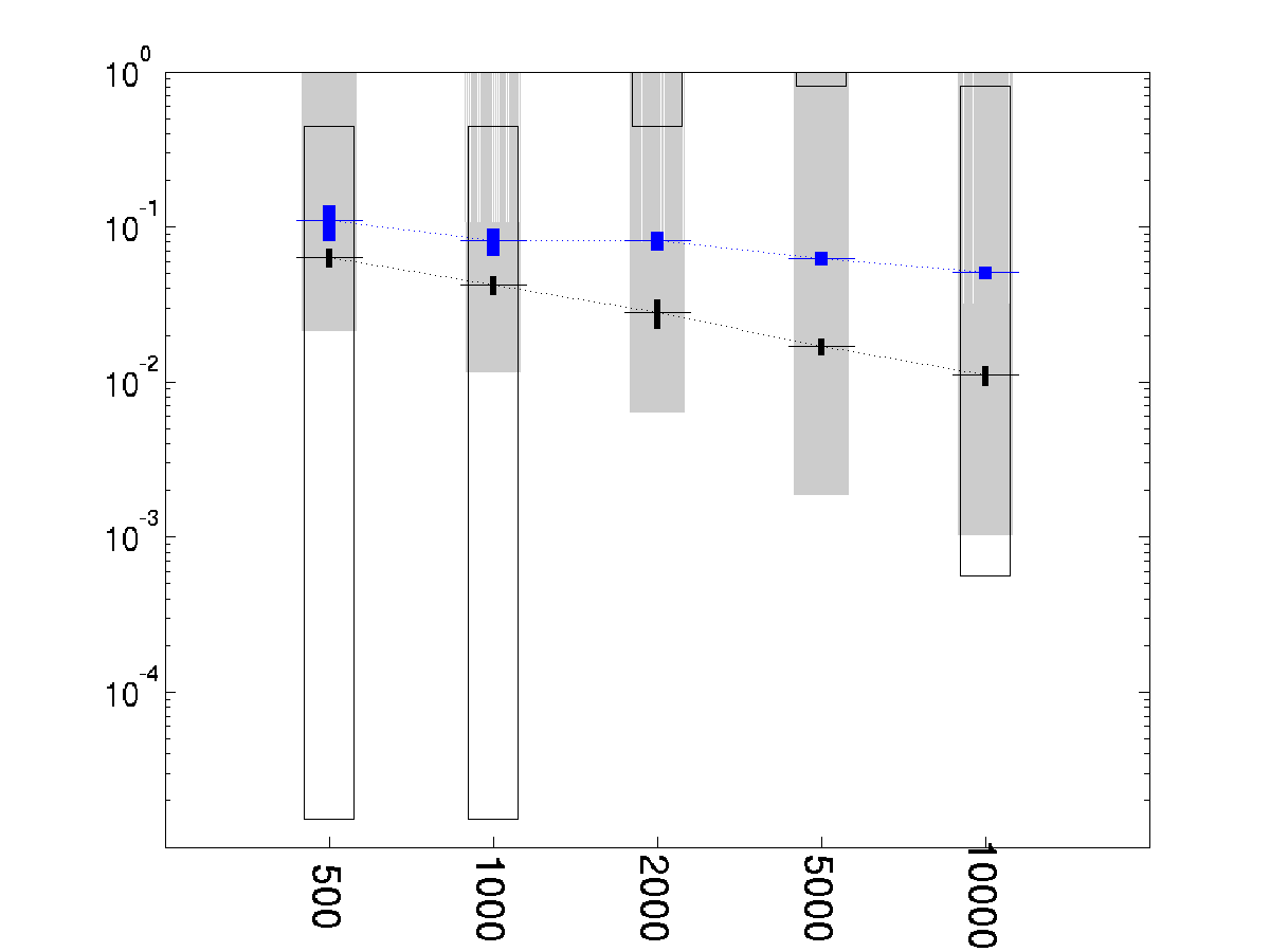
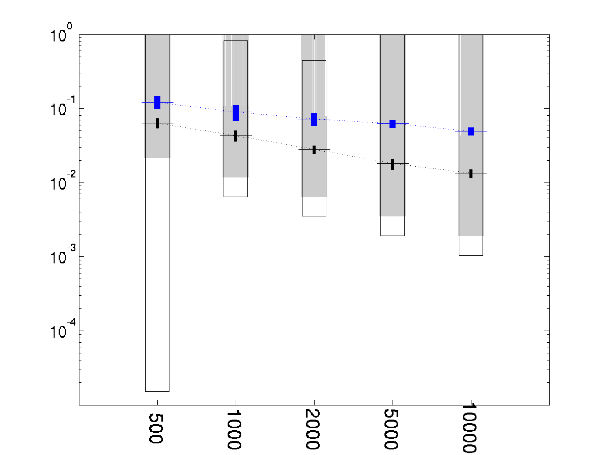
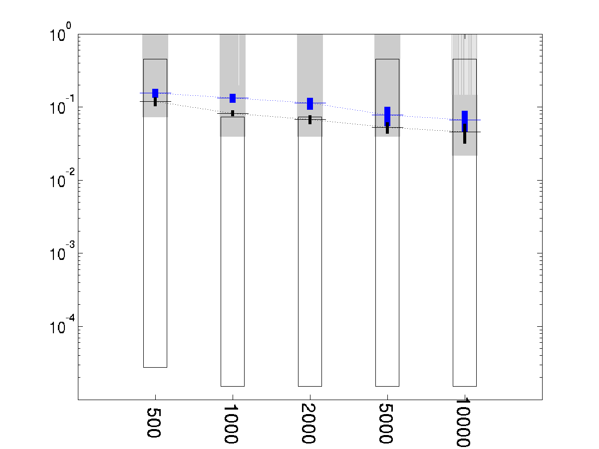
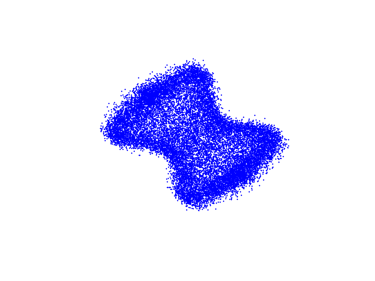
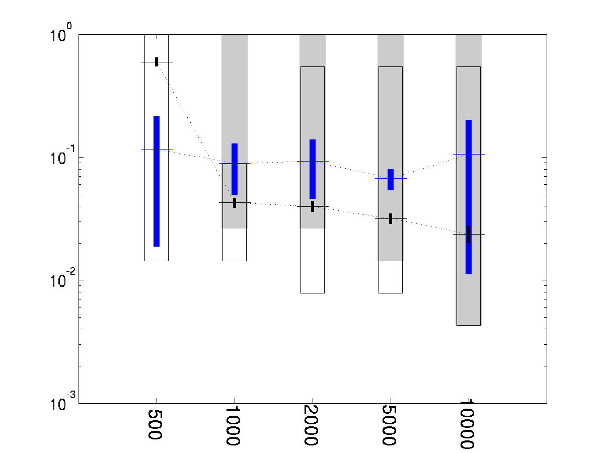
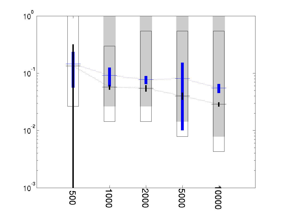
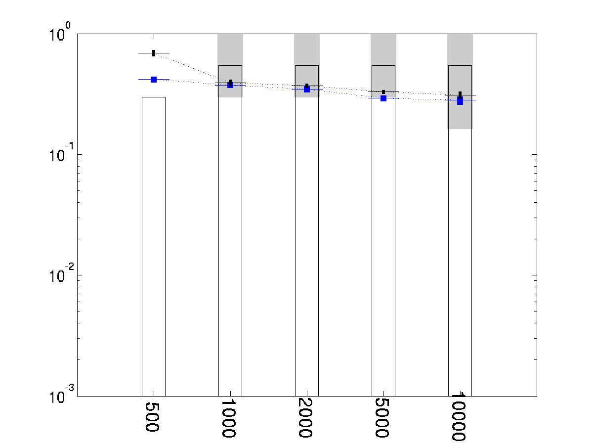
Figure 1: Estimates $\hat{\epsilon}$ (mean and standard deviation over 10 runs) on the dome and hourglass data, vs sample sizes $N$ for various noise levels $\sigma$; $d^{\prime}=2$ is in black and $d^{\prime}=1$ in blue. In the background, we also show as gray rectangles, for each $N,\sigma$ the intervals in the $\epsilon$ range where the eigengaps of local SVD indicate the true dimension, and, as unfillled rectangles, the estimates proposed by Chen et al. (2011) for these intervals.

Effects of $d^{\prime}$, noise and $N$. The estimation results for $\epsilon$ are presented in Figure 1. As mentioned before, one could choose to optimize the distortion in any number of dimensions $d^{\prime}$ not exceeding the intrinsic dimension $d$. Let $\hat{\epsilon}_{d^{\prime}}$ denote the estimate obtained from a $d^{\prime}$ dimensional metric matching. We note a few interesting things. First, when $d_{1}<d_{2}$, typically $\hat{\epsilon}_{d_{1}}>\hat{\epsilon}_{d_{2}}$, but the values are of the same order (a ratio of about 2 in the synthetic experiments). The explanation is that, at $\epsilon$ values near the optimal one, chosing $d^{\prime}<d$ directions in the tangent plane will select a subspace aligned with the “least curvature” directions of the manifold, if any exist, or with the “least noise” in the random sample. In these directions, the data will tolerate more smoothing, which results in larger $\hat{\epsilon}$. The variance of $\hat{\epsilon}$ observed is due to randomness in the subsample $N^{\prime}$ used to evaluate the distortion. The optimal $\epsilon$ decreases with $N$ and grows with the noise levels, reflecting the balance it must find between variance and bias. Note that for the hourglass data, the highest noise level of $\sigma=0.1$ is an extreme case, where the original manifold is almost drowned in the 13-dimensional noise. Hence, $\epsilon$ is not only commensurately larger, but also stable between the two dimensions and runs. This reflects the fact that $\epsilon$ captures the noise dimension, and its values are indeed just below the noise amplitude of $0.1\sqrt{13}$. The dome data set exhibits the same properties discussed previously, showing that our method is effective even for manifolds with border.

Could $\hat{\epsilon}$ be used to improve the estimation of the intrinsic dimension $d$ by the CLMR Chen et al. (2011) method? The CLMR method of estimating the intrinsic dimension $d$ has two components: first, it performs local SVD around each data point at a variety of scales $\epsilon$ (this is akin to our weighted tangent plane projections); then, it finds a range of scales in $\epsilon$ space, which we shall call the CLMR range, where the largest eigengap is the $d$-th eigengap. The $d$ is estimated by finding the largest eigengap somewhere in the CLMR range.

We computed the CLMR ranges both using the method of Chen et al. (2011) (unfilled rectangles in Figure 1) and the ground truth ranges (grey rectangles). As can be seen, our $\hat{\epsilon}$ estimate always lie in within the true ranges, meaning that if we computed the eigengaps at $\hat{\epsilon}$, we would find the true $d$, provided that such a range exists. See Chen et al. (2011) for a more detailed discussion of the limitations of this method in e.g. high-dimensional noise. In contrast, the CLMR ranges only partially overlap with the true ranges. We also found that the CLMR method, which is based on finding the “first descents” of the singular values, can be unreliable in that it may not find an upper or a lower limit to the interval. Figure 2 illustrates this phenomenon for the data set used in the semi-supervised experiments described below. Note that the CLMR method depends on a parameter $K$ to be set by the user, and we gave it the optimal $K$ for these data. Figure 2 (a) shows the distortion ${D}$ that our algorithm minimizes to find the optimal $\epsilon$ for the given data set. Figure 2 (b) illustrates the range of $\epsilon$ chosen by the CLMR method. The CLMR range is $[\epsilon_{1},\epsilon_{2}]$ with $\epsilon_{1}$ the smallest $\epsilon$ value for which $\lambda_{K+1}$ is non-increasing and $\epsilon_{2}$ the smallest value for which $\lambda_{1}$ is non-decreasing. For this particular data set, the CLMR range is approximately $[100,\,300]$ for $K>1$ ($K$ is an upper bound on the intrinsic dimension $d$ of the data). Hence, the CLMR method would choose an $\hat{\epsilon}$ of at least 100 (200 if the middle of the CLMR interval is used).

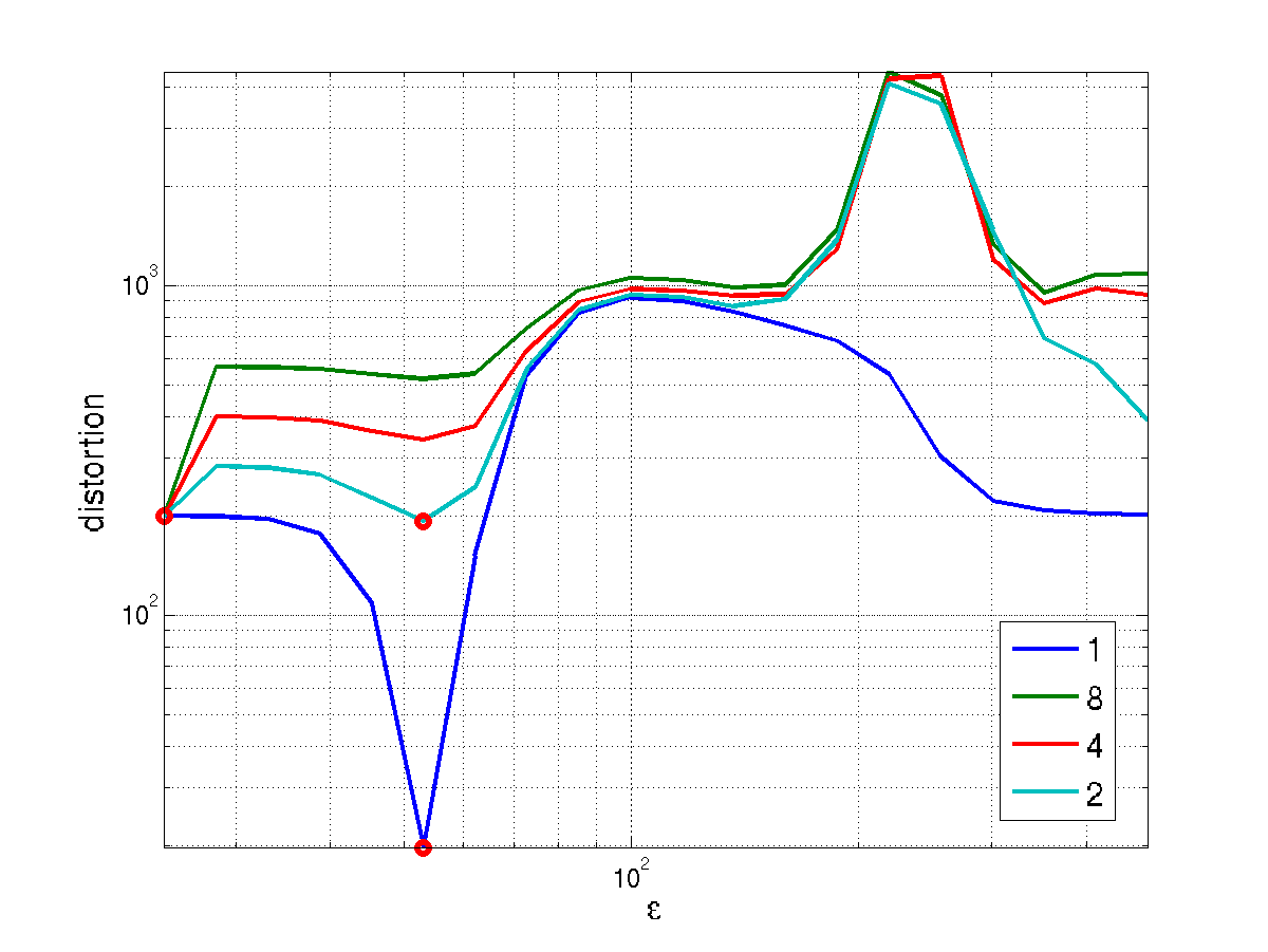
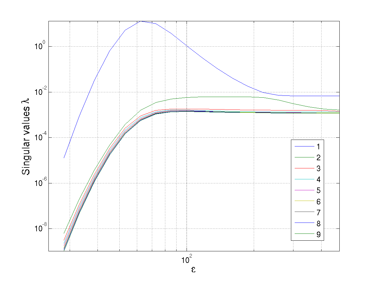
Figure 2: COIL data set (a) costs $\hat{{D}}$ for one sample of $N^{\prime}=200$ and $d^{\prime}=1,\,2,\,4\,8$, showing pronounced minimum at $\hat{\epsilon}=53.1$ for $d^{\prime}=1$ (the lowest curve) and a weaker minimum for $d^{\prime}=2$; the range of $\epsilon$ searched was $[24,\,482]$ (b) the nine largest singular values of local SVD versus $\epsilon$. We do not know the intrinsic dimension of these high-dimensional data. The figure shows why using a low dimensional projection, e.g. $d^{\prime}=1$ may be a practical strategy. One sees also that chosing $\epsilon$ by the CLMR will result in values of at least $100-300$, depending which parameter $K>1$ is chosen. The value chosen by crossvalidation is 54.

Experiments with Smoothing. To investigate whether the $\hat{\epsilon}$ values chosen by our algorithm were “good” values for manifold learning in noise, we sampled $N$ points from the hourglass with no noise added, and we formed the sample $X^{*}$. Then we added 13-dimensional noise of amplitude $\sigma$ as described above, obtaining the data set $X$, where each point $i$ of $X$ is the noisy version of point $i$ in $X^{*}$. We embedded $X$ and $X^{*}$ into 3 dimensions using the same method (Laplacian Eigenmaps), obtaining coordinates $\phi_{\epsilon,i}$ and $\phi^{*}_{\epsilon^{*},i}$, respectively, for each point $i$. We aligned the two embeddings by the Procrustes method and calculated the RMS error $\delta_{\epsilon,\epsilon^{*}}$ and $\delta_{\epsilon}=\min_{\epsilon^{*}}\delta_{\epsilon,\epsilon^{*}}$.

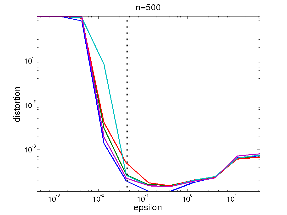
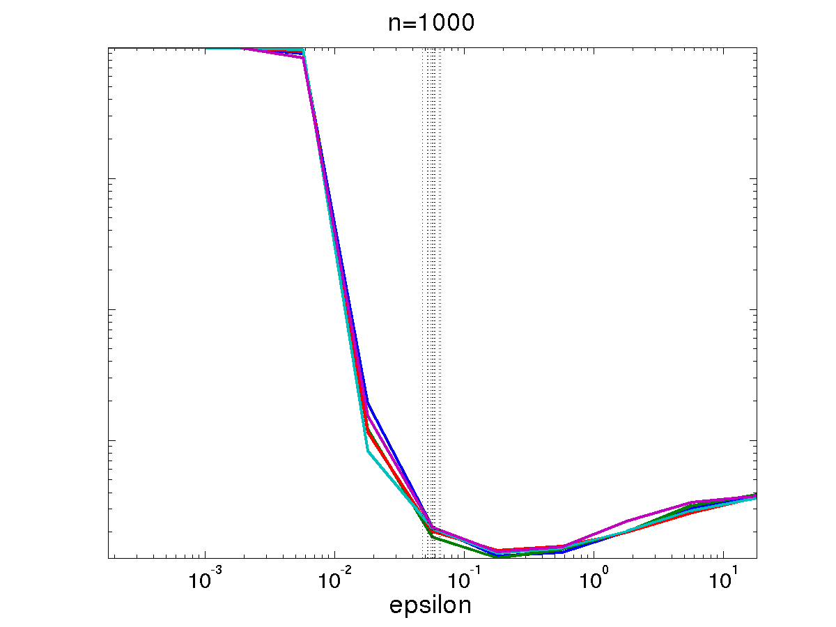
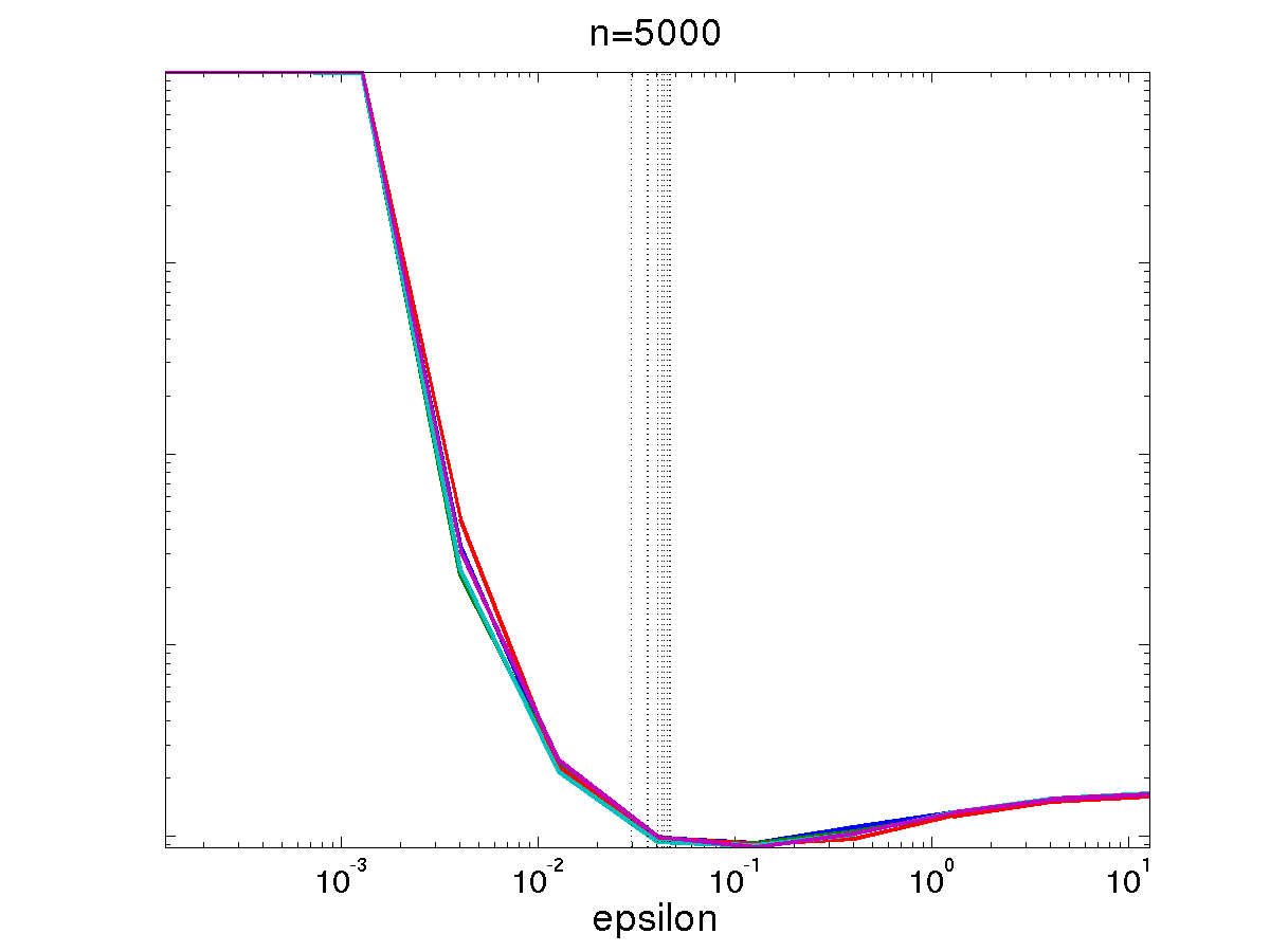
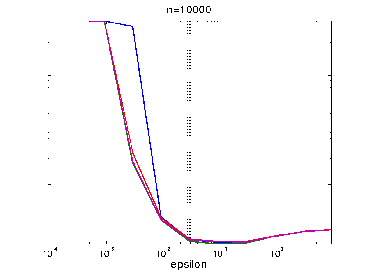
Figure 3: Distortions between embedding of noisy and noiseless manifold data, for various $\epsilon$ values and sample sizes $N$. The manifold is the hourglass embedded in 3D by Laplacian Eigenmap, data in 13 dimensions, noise with $\sigma=0.001$; $\epsilon$ is the scale for the noisy data embedding, and the distortion shown is the lowest over all $\epsilon^{*}$ values for the noiseless data embedding; there were 5 replications in each experiment. The vertical lines are the same $\hat{\epsilon}$ from Figure 1 (10 replicates).

In Figure 3, we show $\delta_{\epsilon}$ vs. $\epsilon$ (as ground truth) along with $\hat{\epsilon}$ obtained by our method (GC ). Our $\hat{\epsilon}$ always finds a region of low $\delta_{\epsilon}$, with a slight but systematic tendency to undershoot. Thus, the experiment supports the case for choosing $\hat{\epsilon}$ by (9) in unsupervised manifold learning, even when noise is present (for which there is yet no theory).

Semi-supervised Learning (SSL) with Real Data. In this set of experiments, the task is classification on the benchmark SSL data sets proposed by Chapelle et al. (2006). This was done by least-square classification, similarly to Zhou and Belkin (2011), after choosing the optimal bandwidth by one of the methods below.

• Minimize Test Error, i.e. “cheat” in an attempt to get an estimate of the “ground truth”.

• Cross-validation We split the training set (consisting of 100 points in all data sets) into two equal groups; we use simulated annealing to minimize the highly non-smooth cross-validation classification error.

• Minimize the reconstruction error We cannot use the method of Chen and Buja (2009) directly, as it requires an embedding, so we minimize reconstruction error based on the heat kernel weights w.r.t. $\epsilon$ (this is reminiscent of LLE Saul and Roweis (2003)): $\mathcal{R}(\epsilon)=\sum_{i=1}^{n}\left|\left|x_{i}-\sum_{j\neq i}\frac{w_{\epsilon}(x_{i},x_{j})}{\sum_{l\neq i}w_{\epsilon}(x_{i},x_{l})}x_{j}\right|\right|^{2}$

Our method is denoted GC  for Geometric Consistency; we evaluate straighforward GC, that uses the dual Riemannian metric, and a variant that includes the matrix inversion in Algorithm 1 denoted GC^-1.

	TE	CV	Rec	GC-1	GC
Digit1	0.67$\pm$0.08	0.80$\pm$0.45	0.64	0.74	0.74
	$[0.57,0.78]$	$[0.47,1.99]$
USPS	1.24$\pm$0.15	1.25$\pm$0.86	1.68	2.42	1.10
	$[1.04,1.59]$	$[0.50,3.20]$
COIL	49.79$\pm$6.61	69.65$\pm$31.16	78.37	216.95	116.38
	$[42.82,60.36]$	$[50.55,148.96]$
BCI	3.4$\pm$3.1	3.2$\pm$2.5	3.31	3.19	5.61
	$[1.2,8.9]$	$[1.2,8.2]$
g241c	8.3$\pm$ 2.5	8.8$\pm$3.3	3.79	7.37	7.38
	$[6.3,14.6]$	$[4.4,14.9]$
g241d	5.7$\pm$ 0.24	6.4$\pm$1.15	3.77	7.35	7.36
	$[5.6,6.3]$	$[4.3,8.2]$

Table 1: Estimates of $\epsilon$ by methods presented for the six SSL data sets used, as well as TE. For TE and CV, which depend on the training/test splits, we report the average, its standard error, and range (in brackets below) over the 12 splits.

	CV	Rec	GC-1	GC
Digit1	3.32	2.16	2.11	2.11
USPS	5.18	4.83	12.00	3.89
COIL	7.02	8.03	16.31	8.81
BCI	49.22	49.17	50.25	48.67
g241c	13.31	23.93	12.77	12.77
g241d	8.67	18.39	8.76	8.76

		$d^{\prime}$=1	$d^{\prime}$=2	$d^{\prime}$=3
Digit1	GC-1	0.74	0.29	0.30
	GC	0.74	0.77	0.78
USPS	GC-1	2.42	2.31	3.88
	GC	1.10	1.16	1.18
COIL	GC-1	116	87.4	128
	GC	187	179	187
BCI	GC-1	3.32	3.48	3.65
	GC	5.34	5.34	5.34
g241c	GC-1	7.38	7.38	7.38
	GC	7.38	9.83	9.37
g241d	GC-1	7.35	7.35	7.35
	GC	7.35	9.33	9.78

Table 2: Left panel: Percent classification error for the six SSL data sets using the four $\epsilon$ estimation methods described. Right panel: $\epsilon$ obtained for the six datasets using various $d^{\prime}$ values with GC  and GC^-1 . $\hat{\epsilon}$ was computed for $d$=5 for Digit1, as it is known to have an intrinsic dimension of 5, and found to be 1.162 with GC  and 0.797 with GC^-1 .

Across all methods and data sets, the estimate of the bandwidth that was furthest away from the “optimal” value determined by TE led to the highest classification error, see left panel of Table 2. This confirms that performance in classification when using a Laplacian-based regularizer is quite sensitive to the estimate of the bandwidth of the Laplacian and lends legitimacy to our attempt at finding a better, more principled method for doing so.

Across five of the six data sets, cross-validation did not perform as well as the GC-based methods, and took 2 to 6 times longer to compute. Further, the CV estimates of $\epsilon$ in each of the 12 training sets within a data set were highly variable, with standard errors often of the same order as the estimated values themselves. This suggests that CV tends to overfit rather than find values that generalize well.

Effect of Dimension $d^{\prime}$. One of the inputs required for computing the distortion of (8) is $d$, the intrinsic dimension of $\mathcal{M}$. In most cases, $d$ is not known, and we do not offer a new method for estimating it. However, we examine how changing the dimension to $d^{\prime}\leq d$ alters our estimate of $\epsilon$ and report our findings in the right panel of Table 2.

The right panel of table 2 shows that the $\hat{\epsilon}$ for different $d^{\prime}$ values are close, even though we search over a range of two orders of magnitude. Even for g241c and g241d, which were constructed so as to not satisfy the manifold hypothesis, our method does reasonably well at estimating $\epsilon$. That is, our method finds the $\hat{\epsilon}$ for which the Laplacian encodes the geometry of the data set irrespective of whether or not that geometry is lower-dimensional.

Overall, we have found that using $d^{\prime}=1$ is most stable, and that adding more dimensions introduces more numerical problems: it becomes more difficult to optimize the distortion as in (9), as the minimum becomes shallower. In our experience, this is due to the increase in variance associated with adding more dimensions. Using one dimension probably works well because the wlPCA selects the dimension that explains the most variance and hence is the closest to linear over the scale considered. Subsequently, the wlPCA moves to incrementally “shorter” or less linear dimensions, leading to more variance in the estimate of the tangent plane.

6 Discussion

In manifold learning, supervised and unsupervised, estimating the graph versions of Laplacian-type operators is a fundamental task. We have provided a principled method for selecting the parameters of such operators, and have applied it to the selection of the bandwidth/scale parameter $\epsilon$. Moreover, our method can be used to optimize any other parameters used in the graph Laplacian; for example, $k$ in the $k$-nearest neighbors graph, or - more interestingly - the renormalization parameter $\lambda$ Coifman and Lafon (2006) of the kernel. The latter is theoretically equal to 1, but it is possible that it may differ from 1 in the finite $N$ regime. In general, for finite $N$, a small departure from the asymptotic prescriptions may be beneficial - and a data-driven method such as ours can deliver this benefit.

By imposing geometric self-consistency, our method estimates an intrinsic quantity of the data. GC  is also fully unsupervised, aiming to optimize a (lossy) representation of the data, rather than a particular task. This is an efficiency if the data is used in an unsupervised mode, or if it is used in many different subsequent tasks. Of course, one cannot expect an unsupervised method to always be superior to a task-dependent one. Yet, GC  has shown to be competitive and even superior in experiments with the widely accepted CV. Besides the experimental validation, there are other reasons to consider an unsupervised method like GC  in a supervised task: (1) the labeled data is scarce, so $\hat{\epsilon}$ will have high variance, (2) the CV cost function is highly non-smooth while ${D}$ is much smoother, and (3) when there is more than one parameter to optimize, difficulties (1) and (2) become much more severe.

Our algorithm requires minimal prior knowledge. In particular, it does not require exact knowledge of the intrinsic dimension $d$, since it can work satisfactorily with $d^{\prime}=1$ in many cases.

An interesting problem that is outside the scope of our paper is the question of whether $\epsilon$ needs to vary over $\mathcal{M}$. This is a question/challenge facing not just GC, but any method for setting the scale, unsupervised or supervised. Asymptotically, a uniform $\epsilon$ is sufficient. Practically, however, we believe that allowing $\epsilon$ to vary may be beneficial. In this respect, the GC method, which simply evaluates the overall result, can be seamlessly adapted to work with any user-selected spatially-variable $\epsilon$, by appropriately changing (2) or sub-sampling $\mathcal{D}$ when calculating ${D}$.

Acknowledgments

This work was partially supported by awards IIS-0313339 and EEC-1028725 from NSF.The content is solely the responsibility of the authors and does not necessarily represent the official views of the National Science Foundation. The authors also gratefully acknowledge NSF award IIS-0313339 under which ideas for this research originated.

References

- Aswani et al. (2011) A. Aswani, P. Bickel, and C. Tomlin. Regression on manifolds: Estimation of the exterior derivative. Annals of Statistics, 39(1):48–81, 2011.
- Belkin and Niyogi (2002) M. Belkin and P. Niyogi. Laplacian eigenmaps for dimensionality reduction and data representation. Neural Computation, 15:1373–1396, 2002.
- Belkin and Niyogi (2007) M. Belkin and P. Niyogi. Convergence of laplacians eigenmaps. In Advances in Neural Information Processing Systems (NIPS), 2007.
- Belkin et al. (2006) M. Belkin, P. Niyogi, and V. Sindhwani. Manifold regularization: A geometric framework for learning from labeled and unlabeled examples. Journal of Machine Learning Research, 7:2399–2434, 2006.
- Carter et al. (2007) K. Carter, A. Hero, and R. Raich. De-biasing for intrinsic dimension estimation. In IEEE Workshop on Statistical Signal Processing, pages 601–605, 2007.
- Chapelle et al. (2006) O. Chapelle, B. Schölkopf, A. Zien, and editors. Semi-Supervised Learning. the MIT Press, 2006. URL http://www.kyb.tuebingen.mpg.de/ssl-book.
- Chen et al. (2011) G. Chen, A. Little, M. Maggioni, and L. Rosasco. Some recent advances in multiscale geometric analysis of point clouds. In Wavelets and Multiscale Analysis: Theory and Applications, Applied and Numerical Harmonic Analysis, pages 199–225. Springer, 2011.
- Chen and Buja (2009) L. Chen and A. Buja. Local Multidimensional Scaling for nonlinear dimension reduction, graph drawing and proximity analysis. Journal of the American Statistical Association, 104(485):209–219, 2009.
- Coifman and Lafon (2006) R. R. Coifman and S. Lafon. Diffusion maps. Applied and Computational Harmonic Analysis, 21(1):6–30, 2006.
- Giné and Koltchinskii (2006) E. Giné and V. Koltchinskii. Empirical Graph Laplacian Approximation of Laplace-Beltrami Operators: Large Sample results. High Dimensional Probability, pages 238–259, 2006.
- Goldberg et al. (2008) Y. Goldberg, A. Zakai, D. Kushnir, and Y. Ritov. Manifold Learning: The Price of Normalization. Journal of Machine Learning Research, 9:1909–1939, 2008.
- Hein et al. (2007) M. Hein, J.-Y. Audibert, and U. von Luxburg. Graph Laplacians and their Convergence on Random Neighborhood Graphs. Journal of Machine Learning Research, 8:1325–1368, 2007.
- Lee and Verleysen (2007) J. A. Lee and M. Verleysen. Nonlinear Dimensionality Reduction. Springer Publishing Company, Incorporated, 1st edition, 2007.
- Lee (1997) J. M. Lee. Riemannian Manifolds: An Introduction to Curvature. Springer, New York, 1997.
- Levina and Bickel (2005) E. Levina and P. Bickel. Maximum likelihood estimation of intrinsic dimension. In Advances in Neural Information Processing Systems (NIPS), 2005.
- Perraul-Joncas and Meila (2013) Dominique Perraul-Joncas and Marina Meila. Non-linear dimensionality reduction: Riemannian metric estimation and the problem of geometric recovery. arXiv:1305–7255, 2013.
- Rosenberg (1997) S. Rosenberg. The Laplacian on a Riemannian Manifold. Cambridge University Press, 1997.
- Saul and Roweis (2003) L. Saul and S. Roweis. Think globally, fit locally: unsupervised learning of low dimensional manifold. Journal of Machine Learning Research, 4:119–155, 2003.
- Sindhwani et al. (2007) V. Sindhwani, W. Chu, and S. S. Keerthi. Semi-supervised gaussian process classifiers. In Proceedings of the International Joint Conferences on Artificial Intelligence, 2007.
- Singer (2006) A. Singer. From graph to manifold laplacian: the convergence rate. Applied and Computational Harmonic Analysis, 21(1):128–134, 2006.
- Smola and Kondor (2003) A. J. Smola and I.R. Kondor. Kernels and regularization on graphs. In Proceedings of the Annual Conference on Computational Learning Theory, 2003.
- Ting et al. (2010) D. Ting, L Huang, and M. I. Jordan. An analysis of the convergence of graph laplacians. In International Conference on Machine Learning, pages 1079–1086, 2010.
- von Luxburg et al. (2008) U. von Luxburg, M. Belkin, and O. Bousquet. Consistency of spectral clustering. Annals of Statistics, 36(2):555–585, 2008.
- Yue et al. (2004) H. Yue, M. Tomoyasu, and N. Yamanashi. Weighted principal component analysis and its applications to improve fdc performance. In 43rd IEEE Conference on Decision and Control, 2004.
- Zhou and Belkin (2011) X. Zhou and M. Belkin. Semi-supervised learning by higher order regularization. In The 14th International Conference on Artificial Intelligence and Statistics, 2011.
- Zhu et al. (2003) X. Zhu, J. Lafferty, and Z. Ghahramani. Semi-supervised learning: From gaussian fields to gaussian processes. Technical report, School of Computer Science, Carnegie Mellon University, 2003.