Magnetic field amplification in nonlinear diffusive shock acceleration including resonant and non-resonant cosmic-ray driven instabilities

Abstract

We present a nonlinear Monte Carlo model of efficient diffusive shock acceleration (DSA) where the magnetic turbulence responsible for particle diffusion is calculated self-consistently from the resonant cosmic-ray (CR) streaming instability, together with non-resonant short– and long–wavelength CR–current–driven instabilities. We include the backpressure from CRs interacting with the strongly amplified magnetic turbulence which decelerates and heats the super-alfvénic flow in the extended shock precursor. Uniquely, in our plane-parallel, steady-state, multi-scale model, the full range of particles, from thermal ($\sim$ eV) injected at the viscous subshock, to the escape of the highest energy CRs ($\sim$ PeV) from the shock precursor, are calculated consistently with the shock structure, precursor heating, magnetic field amplification (MFA), and scattering center drift relative to the background plasma. In addition, we show how the cascade of turbulence to shorter wavelengths influences the total shock compression, the downstream proton temperature, the magnetic fluctuation spectra, and accelerated particle spectra. A parameter survey is included where we vary shock parameters, the mode of magnetic turbulence generation, and turbulence cascading. From our survey results, we obtain scaling relations for the maximum particle momentum and amplified magnetic field as functions of shock speed, ambient density, and shock size.
Keywords: acceleration of particles — ISM: cosmic rays — ISM: supernova remnants — magnetohydrodynamics (MHD) — shock waves — turbulence

1. Introduction

The existence of strong, super-alfvénic collisionless shocks in many astrophysical objects, such as supernova remnants (SNRs), extra-galactic radio jets, clusters of galaxies, and compact accreting sources, has been revealed to us by nonthermal radiation produced by relativistic particles. Diffusive shock acceleration (DSA), the most favored acceleration mechanism for producing these relativistic particles (e.g., Jones & Ellison, 1991; Malkov & Drury, 2001), is expected to be efficient and to produce highly non-equilibrium particle populations. A high acceleration efficiency implies strong coupling between the accelerated particle population, the shock structure, and the electromagnetic fluctuations, with a wide range of scales, responsible for scattering the particles, making DSA a difficult nonlinear (NL) problem.

Efficient DSA produces a hard energy spectrum and the backpressure of these high-energy CRs penetrating into the cold incoming plasma creates a precursor with a length-scale on the order of the diffusion length of the highest energy CRs (e.g., Blandford & Eichler, 1987). Imbeded in this precursor is a short-scale, viscous subshock that is largely responsible for heating the plasma and injecting particles into the Fermi mechanism. Basic considerations of momentum and energy conservation require that the production of relativistic particles involving the largest magnetic turbulence scales must impact the injection of thermal particles and the structure of the shock on the smallest ion inertial scales making the shock intrinsically multi-scale.

Because hard spectra can be produced in efficient DSA, CRs with the longest diffusion lengths can escape at an upstream boundary and carry away a sizable fraction of the shock ram pressure (e.g., Ellison et al., 1981; Berezhko & Krymskiĭ, 1988; Berezhko & Ellison, 1999; Caprioli et al., 2010; Ellison & Bykov, 2011; Drury, 2011; Malkov et al., 2012a). This escaping energy flux plays an important role in DSA and must be self-consistently included in determining the shock structure. It will cause the overall shock compression ratio to increase and the escaping CR current is certain to generate turbulence that will serve as seed turbulence for compression and amplification as it is overtaken by the shock (e.g., Blandford & Funk, 2007; Blasi et al., 2007a; Bell et al., 2013).

Global conservation considerations aside, the detailed formation and structure of collisionless shocks is by no means certain. Early on it was suggested that a Weibel-type instability from counter streaming plasma flows could result in the formation of a gas subshock; a narrow region filled with strong magnetic fluctuations deflecting the incoming particles (e.g., Moiseev & Sagdeev, 1963; Tidman & Krall, 1971). This basic picture was supported later by direct spacecraft observations of heliospheric shocks (e.g., Kennel et al., 1984; Tsurutani & Stone, 1985; Gosling et al., 1989).

In addition to observations, hybrid and particle-in-cell (PIC) plasma simulations have investigated collisionless shocks coupled with particle acceleration. To our knowledge, the first plasma simulation to show clear evidence of DSA was the parallel-shock, hybrid simulation of Quest (1988). Since then, a great deal of work with both hybrid and full-particle PIC simulations has been done (see Winske & Quest, 1988; Winske et al., 1990; Ellison et al., 1993; Giacalone et al., 1997; Kato & Takabe, 2008, 2010; Spitkovsky, 2008a, b; Treumann, 2009; Gargaté & Spitkovsky, 2012; Burgess & Scholer, 2013; Caprioli & Spitkovsky, 2013a, and references therein, for a sampling of this large body of work). The direct simulation of the microscopic structure of the shock on scales of a few thousand ion inertial lengths has been extremely important for resolving the microscopic structure of the plasma shock transition and for clearly demonstrating the initialization of the Fermi acceleration process. However, PIC/hybrid simulations are computationally demanding and the runtime, box size, number of particles, and particle momentum range that can be simulated are limited. In non-relativistic shock simulations, they are currently limited to two or three decades in the dynamical ranges of the spectra of energetic particles and in the $k$-space of the magnetic fluctuations.

In contrast, models of strong MFA applicable to SNRs require dynamical ranges for particle momentum and turbulence extending nine or ten decades. Therefore, to capture the nonlinear physics connecting the highest energy CRs to the self-generated, broadband wave turbulence, and to the viscous subshock structure, coarse grained, multi-scale models of the collisionless plasma turbulence generation must be used in addition to the microscopic treatment afforded by PIC/hybrid simulations (see, e.g., Blandford & Eichler, 1987; Malkov & Drury, 2001; Amato & Blasi, 2006; Vladimirov et al., 2008; Kang, 2013; Reville & Bell, 2013).

Different approaches to model the multi-scale nature of DSA in strong non-relativistic shocks are currently underway. Kinetic semi-analytic models (see, e.g., Malkov & Drury, 2001; Völk et al., 2005; Amato & Blasi, 2006; Zirakashvili & Aharonian, 2010; Bykov et al., 2013b; Lee et al., 2013; Schure & Bell, 2013a; Reville & Bell, 2013) perform self-consistent calculations once the injection rate of background particles into the Fermi mechanism is parameterized. These models use various approximations for the particle diffusion coefficient and the MFA. The background plasma is typically modeled with a diffusion-convection equation which incorporates the magnetic field structure. Some recent time-dependent models have been presented by Kang et al. (2012), Zirakashvili & Ptuskin (2012), and Schure & Bell (2013a).

Another approach combines standard MHD equations to describe the background plasma, including the CR current $\mathbf{j_{\mathrm{CR}}}\times\mathbf{B}$ term producing the non-resonant hybrid (NRH) (i.e., Bell) instability, with a Vlasov–Fokker–Planck equation describing the CR distribution function (see Bell, Schure, Reville, & Giacinti, 2013, and references therein).

Here, we use a Monte Carlo technique which allows broadband modeling of nonlinear DSA incorporating both resonant and non-resonant (short– and long–wavelength) current-driven instabilities. This is a plane-parallel, steady-state model extending earlier work by, for example, Jones & Ellison (1991); Ellison et al. (1996); Vladimirov et al. (2006, 2008, 2009). The model gives a consistent account of the amplification of mesoscopic scale fluctuating magnetic fields interacting with superthermal CRs and the NL feedback of particles and fields on the bulk flow is derived from basic energy-momentum conservation laws. By mesoscale, we mean magnetic turbulence with scales between the very short-scale Weibel-type instabilities that determine the subshock structure and are seen in PIC simulations, and the very large-scale turbulence, e.g., Raleigh–Taylor instabilities, seen in hydro or MHD simulations (e.g., Giacalone & Jokipii, 2007; Ferrand et al., 2012; Warren & Blondin, 2013). Weibel and Raleigh–Taylor instabilities are not included in our model.

In contrast to semi-analytic models based on the diffusion-advection equation, which make the diffusion approximation and require an independent injection parameter, thermal particle injection in the Monte Carlo model is achieved self-consistently once the particle mean free path is specified (see §2.7.4). Particles from thermal energies to energies sufficient to capture the essential NL effects expected from CR production in young SNRs, as well as the magnetic turbulence interacting with these particles, are included self-consistently.

The source of the mesoscopic resonant and non-resonant turbulence in DSA is the anisotropy of the distribution function of the energetic particles. Since the Monte Carlo method does not assume near isotropic distributions, no approximation is made concerning the CR distribution. The CR pressure gradient and current are obtained to all orders in the shock precursor. Due to computational limits, more restrictive approximations may be necessary in models based on the Vlasov-Fokker-Planck equation (e.g., Bell et al., 2013).

We calculate the spectra of the magnetic turbulence using the quasi-linear growth rates described in §2.5. The growth rates are derived from a general dispersion relation given by Bykov et al. (2013a). This single dispersion relation accounts for the three main CR-driven instabilities: Bell’s short-scale instability (Bell, 2004, 2005), the resonant streaming instability (see, for example, Achterberg, 1981; Blandford & Eichler, 1987), and the long-wavelength, ponderomotive instability (see Bykov et al., 2011b, 2013a; Schure et al., 2012).

The Monte Carlo simulation solves the full DSA/$\Delta B$/smooth–shock  problem iteratively. Within this process, we calculate the local growth rates at any iteration using the mean magnetic field and the CR-current derived at the previous iteration. Importantly, between any two iterations $\Delta B/B<1$ so we converge to an amplified magnetic field $\Delta B(x)\gg B_{0}$, i.e., with rms-amplitudes much larger than the initial magnetic field $B_{0}$, without violating the quasi-linear approximation (see § 2.8).

The spectrum of the mesoscopic magnetic fluctuations depends critically on cascading, i.e., the transfer of turbulent energy from long to short wavelengths (e.g., Vladimirov et al., 2008). If MFA is strong, and local turbulent cascading parallel to the mean field is suppressed, as expected in MHD turbulence, then the turbulence spectrum will contain one or more discrete peaks (see Vladimirov et al., 2009; Bykov et al., 2011a, and Section 2.8 below). We show, however, that critical aspects of DSA, such as the particle distribution function, are relatively insensitive to cascading. This effect is discussed in detail in §3.1.

In what follows we emphasize the complex, coupled nature of the problem necessitated by the efficient overall acceleration, the wide dynamic range of the CR distribution function, and the equally broadband, self-generated turbulence produced simultaneously by several instabilities. To highlight these effects, we consider acceleration efficiencies where more than 50% of the shock ram kinetic energy is placed in accelerated particles; combined in trapped and escaping CRs. While trapped and escaping CRs are produced together from the shock ram pressure dissipation they have different properties. The escaping CRs contribute immediately to the galactic CR population while the fate of the trapped CRs depends on the shock evolution, which we do not address in our steady-state, plane geometry model. The trapped particles will eventually leave the SNR but only after losing some fraction of their energy to work done on the magnetic field and expanding plasma. Our model is designed to understand the physical effects of efficient DSA in the local vicinity of an extended supernova shock.

Of particular importance is our treatment of the scattering center speed, $v_{\mathrm{scat}}(x)$, relative to the bulk plasma speed, $u(x)$. This is determined from basic conservation considerations without assuming Alfvén waves and we find $|v_{\mathrm{scat}}|$ to be significantly below what Alfvén waves would predict. Finally, a limited parameter survey is given and we discuss the parameters that determine the maximum CR energy a given shock can produce as well as various observational consequences related to the magnetic turbulence spectra we calculate.

2. Model

The basic elements of our plane-parallel, steady-state, Monte Carlo method have been discussed in a number of previous papers (e.g., Jones & Ellison, 1991; Ellison et al., 1996, 2013). Support for its general validity comes from detailed comparisons with in situ spacecraft observations of particle acceleration at heliospheric shocks (e.g., Blandford & Eichler, 1987; Ellison et al., 1990b; Baring et al., 1997), as well as from direct comparison with hybrid plasma simulations (Ellison et al., 1993). While early versions of the Monte Carlo code asummed simple forms for the particle diffusion, we continue here an extensive generalization of the code to include magnetic turbulence generation and self-consistent diffusion (e.g., Vladimirov et al., 2006, 2008, 2009).

The Monte Carlo code includes the following main elements:
$\bullet$ thermal leakage injection self-consistently coupled to DSA where some fraction of shock-heated thermal particles re-cross the subshock and gain additional energy;
$\bullet$ shock-smoothing where the pressure from superthermal particles in the shock precursor slows and heats the incoming plasma upstream of the viscous subshock;
$\bullet$ CR escape at an upstream free escape boundary (FEB);
$\bullet$ a determination of the overall shock compression ratio $R_{\mathrm{tot}}$, taking into account escaping CRs and the modification of the equation of state from the production of relativistic particles;
$\bullet$ fluctuating magnetic fields simultaneously calculated from resonant, short-, and long-wavelength instabilities generated from the CR current and pressure gradient in the shock precursor;
$\bullet$ momentum and position dependent particle diffusion calculated from the self-generated magnetic fields;
$\bullet$ a consistent determination of the local scattering center speed relative to the bulk plasma; and,
$\bullet$ nonlinear spectral energy transfer (i.e., cascading) and dissipation of wave energy into the background plasma. All of these processes are coupled together making a reasonably consistent, albeit complicated, model.

In all that follows, the bulk plasma flow is in the positive $x$-direction with speed $u(x)$ (see Figure 1). The unmodified (i.e., far upstream) shock speed is $u_{0}$ and the downstream plasma speed, in the shock frame, is $u_{2}=u_{0}/R_{\mathrm{tot}}$. In modified shocks, there is a well-defined subshock compression $R_{\mathrm{sub}}=u_{1}/u_{2}$, where $u_{1}$ is the plasma speed immediately upstream of the viscous subshock. Everywhere, the subscript 0 (2) implies far upstream (downstream) values.

2.1. Small Angle Scattering

The position and momentum dependent scattering mean free path, $\lambda_{\mathrm{mfp}}(x,p)$, of a particle is determined from the local diffusion coefficient $D(x,p)$. A particle moves for a time $\delta t$ and then scatters elastically and isotropically in the local frame through a small angle $\theta_{\mathrm{scat}}\leq\sqrt{6\delta t/t_{c}}$, where $t_{c}=\lambda_{\mathrm{mfp}}/v_{p}\gg\delta t$ (see Ellison, Jones, & Reynolds, 1990a). At this new $x$-position, the particle will have changed momentum because of the converging bulk flow. For the next $\delta t$, $\lambda_{\mathrm{mfp}}$ is updated from the new local $D(x,p)$ and the scattering process is repeated: the particle executes a random walk on a six-dimensional sphere in space and momentum in an ever changing magnetic and bulk flow background. This continues until the particle leaves the shock either by convecting far downstream or escaping at the upstream FEB.

2.2. Thermal Leakage Injection

A well-defined, essentially discontinuous subshock with a subshock compression ratio $R_{\mathrm{sub}}<R_{\mathrm{tot}}$ is always present in our smooth-shock solutions. As thermal particles injected upstream cross the subshock and scatter in the downstream flow they gain enough energy so $v_{p}>u_{2}$ for some fraction of the population depending on the shock Mach number. By virtual of random scatterings in the downstream region, some $v_{p}>u_{2}$ particles will re-cross the subshock into the precursor, gain additional energy, and enter the first-order Fermi acceleration process. This simple form of thermal leakage injection assumes the subshock is transparent and ignores the possible existence of a cross-shock potential or other effects from large amplitudes waves that may occur at the subshock (see, for example, Kato & Takabe, 2010, for PIC results showing the shock transition region).

The injection scheme requires no superthermal seed particles and is entirely defined within the Monte Carlo scattering assumptions of Section 2.1. Since the subshock strength and the downstream flow speed (via $R_{\mathrm{tot}}$) are determined self-consistently with the global shock properties, the injection rate is coupled to DSA through the conservation conditions we discuss below. No “injection parameter” is needed to model injection from the thermal population.

2.3. Mass-Energy-Momentum Conservation

In our steady-state, plane-parallel shock, the conservation of mass flux is given by

$$\rho(x)u(x)=\rho_{0}u_{0}\ ,$$ (1)

where $\rho(x)$ is the plasma density and $\rho_{0}u_{0}$ is the far upstream mass flux. The momentum flux conservation is given by

$$\Phi^{\mathrm{part}}_{P}(x)+P_{w}(x)=\Phi_{P0}\ ,$$ (2)

where $\Phi^{\mathrm{part}}_{P}(x)$ is the particle momentum flux, $P_{w}(x)$ is the momentum flux carried by the magnetic waves, and $\Phi_{P0}$ is the far upstream momentum flux, i.e., upstream from the free escape boundary where the interstellar magnetic field is $B_{\mathrm{ISM}}$.

Separating the contributions from the thermal and accelerated particles we have

$$\rho(x)u^{2}(x)+P_{\mathrm{th}}(x)+P_{\mathrm{cr}}(x)+P_{w}(x)=\Phi_{P0}\ ,$$ (3)

where $P_{\mathrm{th}}(x)$ is the thermal particle pressure and $P_{\mathrm{cr}}(x)$ is the accelerated particle pressure. A particle is “accelerated” if it has crossed the subshock more then once and even though we use the subscript “CR”, the vast majority of accelerated particles will always be non-relativistic. Of course, if the acceleration is efficient, a large fraction of the pressure may be in relativistic particles.

The energy flux conservation law is

$$\Phi^{\mathrm{part}}_{E}(x)+F_{w}(x)=\Phi_{E0}\ ,$$ (4)

where $\Phi^{\mathrm{part}}_{E}(x)$ and $F_{w}(x)$ are the energy fluxes in particles and magnetic field correspondingly, and $\Phi_{E0}$ is the energy flux far upstream. Taking into account particle escape at an upstream FEB, this can be re-written as

$$\frac{\rho(x)u^{3}(x)}{2}+F_{\mathrm{th}}(x)+F_{\mathrm{cr}}(x)+F_{w}(x)+Q_{\mathrm{esc}}=\Phi_{E0}\ ,$$ (5)

where $F_{\mathrm{th}}(x)$ is the internal energy flux of the background plasma, $F_{\mathrm{cr}}(x)$ is the energy flux of accelerated particles, and $Q_{\mathrm{esc}}$ is the energy flux of particles that escape at the upstream FEB (note that $Q_{\mathrm{esc}}$ is defined as positive even though CRs escape moving in the negative $x$-direction).

As seen in Figure 6 in Ellison et al. (1990b) or Figure 8 in Vladimirov et al. (2006) or Figure 2 in Caprioli & Spitkovsky (2013a), to give just three examples, the separation between “thermal” particles and “accelerated” particles in a shock undergoing DSA is not necessarily well defined. Furthermore, energy exchange between the thermal and superthermal populations is certain to occur through non-trivial wave-particle interactions. Nevertheless, the bulk of the plasma mass will always be in quasi-thermal background particles and the internal energy flux of this background plasma can be expressed as

$$F_{\mathrm{th}}(x)=u(x)\gamma_{g}P_{\mathrm{th}}(x)/(\gamma_{g}-1)\ ,$$ (6)

where $\gamma_{g}=5/3$ is the adiabatic index of the background plasma.

2.4. Magnetic Turbulence Generation and Dissipation

We calculate the magnetic turbulence generated by the CR current, $J_{\mathrm{cr}}$, and pressure gradient, $dP_{\mathrm{cr}}/dx$, which simultaneously drive resonant, short–, and long–wavelength instabilities.

2.4.1 Energy Balance Equations

The spectral energy density of the magnetic fluctuations $W(x,k)$, where $Wdk$ is the amount of energy in the wavenumber interval $dk$ per unit spatial volume, can be calculated including cascading. The energy balance equation is

$$\frac{\partial{\cal F}_{w}(x,k)}{\partial x}+\frac{\partial\Pi(x,k)}{\partial k} = u(x)\frac{\partial{\cal P}_{w}(x,k)}{\partial x}+$$ (7)

$$G(x,k)-{\cal L}(x,k)\ ,$$

where $\Pi(x,k)$ is the flux of magnetic energy through $k$-space towards larger $k$, and $G(x,k)$ and ${\cal L}(x,k)$ are the spectral energy growth and the dissipation rates, respectively. The turbulence energy flux and pressure are given by

$$F_{w}(x)=\int^{k_{\mathrm{max}}}_{k_{\mathrm{min}}}{\cal F}_{w}(x,k)dk$$ (8)

and

$$P_{w}(x)=\int^{k_{\mathrm{max}}}_{k_{\mathrm{min}}}{\cal P}_{w}(x,k)dk\ ,$$ (9)

where the energy flux and pressure from the CR-current driven fluctuations are given in equations (10) and (11) below. Equation (7) differs from equation (1) in Vladimirov et al. (2009) in that we now explicitly include adiabatic compression of the magnetic turbulence energy density.

The energy flux and pressure from the CR-current driven fluctuations that are included in equations (3) and (5) are defined as

$${\cal F}_{w}(x,k)=u(x)\frac{\left(\left|\varphi(k)\right|^{2}+2\right)}{\left(\left|\varphi(k)\right|^{2}+1\right)}W(x,k)\ ,$$ (10)

and

$${\cal P}_{w}(x,k)=\frac{1}{\left(\left|\varphi(k)\right|^{2}+1\right)}W(x,k)\ .$$ (11)

For the case of CR-driven modes in a highly conducting plasma with frozen-in magnetic fields, the velocity and field amplitudes of a harmonic perturbation are connected through the relation

$$\delta\mathbf{u}_{k}=\varphi(k)\frac{\delta\mathbf{B}_{k}}{\sqrt{4\pi\rho}}\ ,$$ (12)

where $\varphi(k)$, with a complicated derivation, can be determined from the dispersion equation (20) given below and the mode polarizations. For simplicity, we only present results for $\varphi(k)=1$ (as is the case for Alfvén modes), to be compared with those in Vladimirov et al. (2009), but we have verified that the resulting spectra of magnetic fields and particles do not vary significantly for the range $0.1<|\varphi(k)|<10$.

Integrating equation (7) from $k_{\mathrm{min}}$ to $k_{\mathrm{max}}$ we obtain

$$\frac{dF_{w}(x)}{dx} = u(x)\frac{dP_{w}(x)}{dx}+$$ (13)

$$\int^{k_{\mathrm{max}}}_{k_{\mathrm{min}}}G(x,k)dk-L(x)\ .$$

The limits $k_{\mathrm{min}}$ and $k_{\mathrm{max}}$ are chosen to be outside the range containing a maximum scale determined by MFA and a minimum scale determined by dissipation. For these limits, the $\Pi(x,k)$ term in equation (7) vanishes.

For Kolmogorov-type cascading, the energy flux is redistributed over the energy scale but the total energy flux density, integrated over wavenumbers is conserved. Therefore, the total dissipation rate at any position $x$ is

$$L(x)=\int^{k_{\mathrm{max}}}_{k_{\mathrm{min}}}{{\cal L}(x,k)}\,dk\ .$$ (14)

We note that Kolmogorov-type cascade models have been successful at explaining the spectra of locally isotropic, incompressible turbulence in non-conducting fluids observed in experiments and simulations (e.g., Biskamp, 2003). However, it is uncertain how spectral energy transfer operates in a collisionless shock precursor with a CR current strong enough to modify the MHD modes, and in the presence of strong magnetic turbulence. In weak MHD turbulence, cascading was shown to be anisotropic (e.g., Goldreich & Sridhar, 1997): harmonics with wavenumbers transverse to the mean magnetic field experience a Kolmogorov-like cascade, while the cascade in wavenumbers parallel to the mean field is suppressed.

2.5. Growth Rates of CR-Driven Instabilities

Self-generated magnetic turbulence is a key ingredient for DSA and the production of galactic cosmic rays (e.g., Bell, 1978; Blandford & Eichler, 1987; Jones & Ellison, 1991; Malkov & Drury, 2001; Parizot et al., 2006; Bykov et al., 2012; Schure et al., 2012). Most analytical models that calculate MFA (e.g., Bell, 2004; Pelletier et al., 2006; Amato & Blasi, 2009a; Bykov et al., 2011b, 2013a) assume the following “homogeneous” form for the CR distribution function in the local rest frame of the upstream flow:

$$f_{0}(\mathbf{p})=\frac{n_{\mathrm{cr}}}{4\pi}N(p)\left[1+\frac{3u_{0}}{c}\mu\right],$$ (15)

where $n_{\mathrm{cr}}$ is the concentration of CRs, $u_{0}$ is the shock velocity, $\mathbf{p}$ is the particle momentum in the plasma frame, $\mu=\cos{\theta}$, and $\theta$ is the particle pitch angle, i.e., the angle between $\mathbf{p}$ and the magnetic field assumed to lie in the $x$-direction. The CR distribution function, $N(p)$, is normalized as $\int_{p_{\mathrm{min}}}^{p_{\mathrm{max}}}N(p)p^{2}dp=1$, where $p_{\mathrm{min}}$ and $p_{\mathrm{max}}$ are the minimum and maximum particle momenta in the CR distribution at the upstream position. In analytic or semi-analytic treatments, $n_{\mathrm{cr}}$ and $u_{0}$ are normally assumed to be position independent and $N(p)$ is often assumed to be a power law.

In the Monte Carlo code, the particle distribution function contains more information than represented by equation (15). It is calculated directly in the modified shock precursor with a varying $n_{\mathrm{cr}}(x)$ and $u(x)$, rather than constant values, and no approximations are made restricting the particle anisotropy. Instead of $f_{0}(\mathbf{p})$, we can use

$$f_{\mathrm{cr}}(x,\mathbf{p})=\frac{n_{\mathrm{cr}}(x)N(x,p)}{4\pi}+\frac{3J^{\mathrm{cr}}(x,p)}{4\pi v_{p}}\mu\ ,$$ (16)

to calculate the local growth rates. Here, $J^{\mathrm{cr}}(x,p)$ is the differential CR current, $v_{p}$ is the particle velocity in the local frame, and $N(x,p)$ is determined self-consistently with the shock structure and will not be a power law in the shock precursor. The full CR current (for now we consider only protons) is

$$J_{\mathrm{cr}}(x)=e\int_{p_{\mathrm{min}}(x)}^{p_{\mathrm{max}}}J^{\mathrm{cr}}(x,p)\,p^{2}dp\ ,$$ (17)

and this is used to calculate the CR-driven instabilities. Note that $J^{\mathrm{cr}}(x,p)$ only contains superthermal particles and $p_{\mathrm{min}}$ depends on $x$, increasing as the observation position moves further upstream from the subshock.

At any $x$-position in the precursor, we use local Monte Carlo  values for $n_{\mathrm{cr}}(x)$, $u(x)$, and $J_{\mathrm{cr}}(x)$ to calculate the dispersion relation, ignoring effects from spatial gradients in our “local homogeneous” approximation. Specifically, the growth rates for the three CR-driven instabilities are derived from the dispersion relation for modes propagated along the mean magnetic field in the magnetized background plasma. This dispersion relation, which includes the short–wavelength Bell instability (i.e., Bell, 2004), was derived in Bykov et al. (2011b, 2013a), and is

$$\omega^{2}\mp\omega ikk_{c}\frac{\alpha_{t}}{4\pi\rho}\left[\frac{1}{2}\frac{eA(x,k)}{J_{\mathrm{cr}}(x)}+\frac{3}{2}\right]-k^{2}v_{a}^{2}\pm$$

$$\pm kk_{c}v_{a}^{2}\left(1+\frac{\kappa_{t}}{B_{\mathrm{ls}}(x,k^{*})}\right)\left[\frac{eA(x,k)}{J_{\mathrm{cr}}(x)}-1\right]=0,$$ (18)

where $\rho$ is the background plasma density, and the $\pm$ signs, here and in the equations that follow, correspond to the two circularly polarized modes. The mean magnetic field, $B_{\mathrm{ls}}(x,k)$, in the dispersion relations is defined as the sum of the long-wavelength (i.e., large-scale “ls”) harmonics plus the ambient homogeneous field, $B_{0}$, i.e.,

$$B_{\mathrm{ls}}(x,k)=\sqrt{4\pi\int_{k_{\mathrm{min}}}^{k}W(x,k^{{}^{\prime}})dk^{{}^{\prime}}+B_{0}^{2}}\ .$$ (19)

The definitions for $A(x,k)$ (equation 23) and $k^{*}$ (equation 29) are given below and $\alpha_{t}$ and $\kappa_{t}$ are defined in Section 5.1 of Bykov et al. (2011b).

The solution to equation (2.5) is

$$\omega=\left(\pm\sqrt{d^{2}+4b}-d\right)/2\ .$$ (20)

In equations (2.5) and (20),

$$d=\mp ikk_{c}\frac{\alpha_{t}}{4\pi\rho}\left[\frac{1}{2}\frac{eA(x,k)}{J_{\mathrm{cr}}(x)}+\frac{3}{2}\right],$$ (21)

$$b=k^{2}v_{a}^{2}\left[1\mp\frac{k_{c}}{k}\left(1+\frac{\kappa_{t}}{B_{\mathrm{ls}}(x,k^{*})}\right)\left(\frac{eA(x,k)}{J_{\mathrm{cr}}(x)}-1\right)\right],$$ (22)

$$A(x,k)=\int_{0}^{\infty}\sigma(p)J^{\mathrm{cr}}(x,p)p^{2}dp\ ,$$ (23)

$$\sigma(z)=\frac{3}{2z^{2}}+\frac{3}{8z}\left(1-\frac{1}{z^{2}}+\left(\frac{a}{z}\right)^{2}\right)\Psi_{1}-\frac{3a}{2z^{3}}\Psi_{2}$$

$$\mp i\left\{\frac{3}{4z}\left(1-\frac{1}{z^{2}}+\left(\frac{a}{z}\right)^{2}\right)\Psi_{2}-\frac{3a}{2z^{2}}+\frac{3a}{4z^{3}}\Psi_{1}\right\},$$

$$\Psi_{1}(z)=\ln\left[\frac{(z+1)^{2}+a^{2}}{(z-1)^{2}+a^{2}}\right]\,,$$

$$\mathrm{and,}$$

$$\Psi_{2}(z)=\arctan\left(\frac{z+1}{a}\right)+\arctan\left(\frac{z-1}{a}\right)\ .$$

In these equations, $v_{a}=B_{\mathrm{ls}}(x,k)/\sqrt{4\pi\rho(x)}$, $z=kcp/(eB_{\mathrm{ls}})$, $a$ is the collision parameter equal to the ratio of the gyroradius of a CR particle to its mean free path determined by scattering on magnetic fluctuations, and $k_{c}=4\pi|J_{\mathrm{cr}}(x)|/[cB_{\mathrm{ls}}(x,k)]$ is Bell’s critical wavenumber at position $x$ in the precursor.

The effective, self-generated, magnetic field is given by

$$B_{\mathrm{eff}}(x)=\sqrt{4\pi\int_{k_{\mathrm{min}}}^{k_{\mathrm{max}}}W(x,k^{{}^{\prime}})dk^{{}^{\prime}}},$$ (25)

or equivalently,

$$B_{\mathrm{eff}}(x)=\sqrt{B_{\mathrm{ls}}^{2}(x,k_{\mathrm{max}})-B_{0}^{2}}\ .$$ (26)

The total field is $B_{\mathrm{tot}}=B_{\mathrm{ls}}(x,k_{\mathrm{max}})$ so $B_{\mathrm{tot}}^{2}=B_{\mathrm{eff}}^{2}+B_{0}^{2}$. As mentioned above, we assume the ambient ISM field consists of a uniform component $B_{0}=3$ $\mu$G, and a turbulent part generated from the background Kolmogorov turbulence assumed to have a strength such that $B_{\mathrm{Kolm}}=3$ $\mu$G. Therefore, for the ISM, $B_{\mathrm{tot}}\simeq 4.2$ $\mu$G.

2.5.1 Long–wavelength Instability

The plasma fluctuations created by Bell’s short–wavelength instability influence the plasma dynamics and this effect is modeled with the ponderomotive coefficients, $\alpha_{t}$ and $\kappa_{t}$, in equations (21) and (22). These ponderomotive effects result in the long–wavelength plasma instability (LWI) developed by Bykov, Osipov, & Ellison (2011b) and Bykov et al. (2013a).

The ponderomotive coefficients are determined by the mean square of the short-scale magnetic field fluctuations produced by Bell’s instability, i.e.,

$$\kappa_{t}/[B_{\mathrm{ls}}(x,k^{*})]=\pi N_{B}\ ,$$ (27)

and

$$\frac{k_{0}\alpha_{t}}{4\pi\rho}=2\pi\sqrt{\xi}N_{B}v_{a}\ ,$$ (28)

where $\xi$ is the dimensionless mixing length of the short-scale turbulence as defined in Bykov et al. (2011b), $v_{a}$ is the Alfvén speed which is the characteristic speed of the medium, and $N_{B}$, the dimensionless amplitude of the magnetic fluctuations, is defined below. While $N_{B}$ is determined in the Monte Carlo simulation from the CR distribution, $\xi$ is not. In the simulations reported here, we take $\xi=5$ but note that our results are only weakly dependent on $\xi$.

To achieve a solution, we set the ponderomotive coefficients in the dispersion equation (20) equal to zero for wavenumbers $k>k^{*}$, where $k^{*}$ is determined by the effective resonant condition

$$k^{*}c\,p_{\mathrm{min}}(x)=eB_{\mathrm{ls}}(x,k^{*})\ .$$ (29)

At any $x$-position we set $N_{B}(x)$ = 0 for $k^{*}(x)>k_{c}(x)$, where there is no wave growth from Bell’s mode, and we set

$$N_{B}(x)=\frac{\sqrt{B_{\mathrm{ls}}^{2}(x,k_{c})-B_{\mathrm{ls}}^{2}(x,k^{*})}}{B_{\mathrm{ls}}(x,k^{*})}\ ,$$ (30)

for $k^{*}(x)<k_{c}(x,k^{*})$, where Bell’s instability operates. The mode growth rates, $\Gamma(x,k)$, in the turbulence energy balance equation (13), where $G$ is the energy growth rate (see equation 58 below), are connected to the roots of the dispersion equation as

$$\Gamma(x,k)=2\,\mathrm{Im}[\omega(x,k)]\ ,$$ (31)

where the 2 accounts for the fact that the energy in turbulence is proportional to the square of the amplitude of $\Delta B$. At each $x$-position we choose the mode with the maximum value of $\mathrm{Im}[\omega(x,k)]$, if positive.

Because we use the full, anisotropic CR distribution function in equation (2.5) and the substitutions that follow, the dispersion equation (20) simultaneously accounts for the CR-pressure driven resonant streaming instability, and the two CR-current driven instabilities. To our knowledge, this is the first attempt to combine these instabilities in a consistent, broadband shock model.

2.5.2 Dissipation and Fluxes of Particles and Waves

The self-generated turbulence is assumed to suffer viscous dissipation at a rate proportional to $k^{2}$, and the dissipated energy is pumped directly into the thermal particle background. The background plasma energy balance is governed by the plasma compression and the turbulence dissipation rate and obeys the equation

$$\frac{dF_{\mathrm{th}}(x)}{dx}=u(x)\frac{dP_{\mathrm{th}}(x)}{dx}+L(x)\ .$$ (32)

If the heating of the background plasma by the turbulence dissipation is weak [i.e., $L(x)\sim 0$], equations (1), (6), and (32) result in the adiabatic compression of the background plasma.

The results of Vladimirov et al. (2008), which included only the resonant CR-streaming instability for MFA with a variable dissipation rate, demonstrated that even a modest rate of turbulence dissipation can significantly increase the precursor temperature (see Figure 15 below) and that this, in turn, can increase the rate of injection of thermal particles (see also Vladimirov et al., 2009). However, the nonlinear feedback of these changes on the shock structure tend to cancel so that the spectrum of high energy particles is only modestly affected. As described in Vladimirov et al. (2009), we only apply dissipation to our models with cascading.

The relation between the CR pressure gradient and the CR energy flux $F_{\mathrm{cr}}$, can be written as

$$\frac{dF_{\mathrm{cr}}(x)}{dx}=\left[u(x)+v_{\mathrm{scat}}(x)\right]\frac{dP_{\mathrm{cr}}(x)}{dx}\ ,$$ (33)

where $v_{\mathrm{scat}}(x)$ is the scattering center velocity measured in the local frame. This definition is a position dependent generalization of the position independent “wave frame” velocity introduced by Skilling (1971) for CR interactions with hydromagnetic waves. An important feature of the CR-current driven modes is that, in the most interesting cases with $\mathrm{Im}[\omega(k,x)]>kv_{a}$, the scattering center velocity must be substantially less than the Alfvén speed $v_{a}$ in order to achieve energy conservation. This is true whether $B_{0}$ or $B_{\mathrm{ls}}$ is used to calculate $v_{a}$ and is discussed in detail in §2.6.

As follows from equation (10), the energy flux ${\cal F}_{w}(x,k)$ may span the range from $W(x,k)$ to $2\,W(x,k)$, for $\varphi(k)$ between 0 and 1. In our Monte Carlo simulations, we use $\varphi(k)=1$ but our results are not sensitive to $\varphi(k)$. For resonantly generated Alfvén modes, McKenzie & Voelk (1982) derived

$${\cal F}_{w}(x,k)=\left[3u(x)/2+v_{\mathrm{scat}}(x)\right]W(x,k)$$ (34)

and

$${\cal P}_{w}(x,k)=W(x,k)/2\ ,$$ (35)

which corresponds to $\varphi(k)=1$, since the kinetic and magnetic energy densities are exactly equal for Alfvén modes.

2.6. Effective Scattering Center Velocity

The turbulence produced by shock accelerated particles can move relative to the bulk plasma and this movement must be self-consistently included when determining the nonlinear shock structure. If the turbulence is assumed to be Alfvén waves, the scattering center speed can be taken to be the Alfvén speed with the far upstream field, $v_{a0}(x)=B_{0}/\sqrt{4\pi\rho(x)}$, and the turbulence can be calculated in equation (13) in a straightforward fashion using

$$\int^{k_{\mathrm{max}}}_{k_{\mathrm{min}}}G(x,k)dk=-v_{a0}(x)\frac{dP_{\mathrm{cr}}}{dx}\ ,$$ (36)

to model the wave growth.

Equation (36) was obtained by McKenzie & Voelk (1982) assuming (i) that the resonant wave-CR particle interactions are quasi-linear with $\lambda\propto 1/W(x,k)$, and (ii) that the magnetic turbulence is dominated by quasi-linear modes with growth rates $\Gamma(x,k)\ll kv_{a0}$ (for simplicity we only consider modes propagating parallel to the mean magnetic field), and (iii) that the mode growth rate is a linear function of the isotropic part of the distribution function $f(x,p)$. One ambiguity with this approach is the choice of $B$. It is typically chosen as either $B_{0}$ or some fraction of the amplified magnetic field at $x$.

In considering equation (36), however, it must be noted that non-resonant, CR current-driven modes (e.g., Bell, 2004; Bykov et al., 2011b; Schure et al., 2012; Bykov et al., 2013a) have their fastest growth rates when $\Gamma(x,k)>kv_{a0}$ and these modes dominate the magnetic fluctuation spectra. This point can be illustrated in a simple way. Consider just the growth rate of Bell’s instability without the LWI. Then, the solution to equation (2.5) is

$$\omega=\pm\sqrt{v_{a0}^{2}k^{2}+K(k,J^{\mathrm{cr}})}\ ,$$ (37)

where $K(k,J^{\mathrm{cr}})$ is determined by the CR current. This equation can be obtained directly from equation (20) by setting $\alpha_{t}=\kappa_{t}=0$, the two parameters responsible for the LWI. To get equation (36), two conditions must hold. The first is that $\left|K\right|\ll v_{a}^{2}k^{2}$ and therefore the square root in equation (37) can be expanded as

$$\omega\approx\pm v_{a0}k\left(1+\frac{K}{2v_{a0}^{2}k^{2}}\right).$$ (38)

The second condition is that $\Gamma(x,k)$ is a linear function of the distribution function $f(x,p)$. Note that $G(x,k)=\Gamma(x,k)W(x,k)$ is generally assumed in our approach.

While both of these conditions can be fulfilled in the case of weakly growing Alfvén-like turbulence, weak growth is not expected if the CR current is as large as believed to occur in young SNRs. If the CR current is large, and non-resonant current driven instabilities are important, then $\left|K\right|\gg v_{a0}^{2}k^{2}$ and equation (37) simplifies to

$$\omega\approx\pm\sqrt{K}\ ,$$ (39)

that is, $\omega$ is proportional to the square of $K$ rather than proportional to $K$. While $K(k,J^{\mathrm{cr}})$ is a linear function of $f(x,p)$ (if the diffusion approximation is valid), it is clear from equation (39) that the wave growth term $G(x,k)$ is a nonlinear function of $f(x,p)$ for large CR currents.

We believe this reevaluation of the self-generation of turbulence by non-resonant modes is fundamentally important. The non-resonant turbulence has a character quite different from Alfvén waves and we find that equation (36), regardless of the choice of $B$, does not allow for momentum and energy conserving solutions. With the Monte Carlo technique, we obtain consistent solutions by simply generalizing equation (36) to

$$v_{\mathrm{scat}}(x)\frac{dP_{\mathrm{cr}}}{dx}=-\int^{k_{\mathrm{max}}}_{k_{\mathrm{min}}}G(x,k)dk\ ,$$ (40)

assuming there is a single, position dependent, effective scattering speed, and including $v_{\mathrm{scat}}(x)$ in our iterative scheme. Equation (40) is derived using equations (1), (3), (5), (13), (33), and the equation of state of the background plasma.

At each iteration, the $i$-th$+1$ value of the scattering center velocity, $v_{\mathrm{scat}}^{(i+1)}(x)$, is obtained from

$$v_{\mathrm{scat}}^{(i+1)}(x)=-\frac{\int^{k_{\mathrm{max}}}_{k_{\mathrm{min}}}{\Gamma^{(i)}(x,k)W^{(i)}(x,k)}dk}{dP_{\mathrm{cr}}^{(i)}/dx}\ ,$$ (41)

where $\Gamma$, $W$, and $dP_{\mathrm{cr}}/dx$ are all determined in the Monte Carlo simulation in the $i$-th iteration. With equation (41) there is no need to associate $v_{\mathrm{scat}}$ with the Alfvén speed. In the upstream region, accelerated particles are propagated through the shock assuming the scattering center velocity is $u(x)+v_{\mathrm{scat}}(x)$, while the velocity is $u(x)$ for the background thermal particles. Downstream from the shock, we take $v_{\mathrm{scat}}=0$.

An essential and unique element of our calculation is that when the integral in equation (40), with $v_{\mathrm{scat}}$ determined from equation (41), is used to replace the integral in the energy balance equation (7), we make use of the full anisotropic CR distribution function including the pressure gradient and the CR current. Our derivation of $v_{\mathrm{scat}}(x)$ accounts for the anisotropic magnetic modes with dispersive properties (phase and group velocities) determined by both the background plasma and the CR angular and momentum distributions. As we show below (see Figure 18), while the fastest growing CR-driven modes are highly anisotropic, their phase and group velocities are typically strongly sub-alfvénic with $v_{\mathrm{scat}}(x)\ll u(x)$ for all $x$.

Significantly, even though $v_{\mathrm{scat}}(x)$ may be small, it has a strong influence on particle acceleration and must be taken into account to determine a consistent shock structure in the Monte Carlo model. Despite its wide use for many years, we caution that replacing the wave-growth term in equation (13) with equation (36) is a poor approximation when short– and long–wavelength instabilities are taken into account.

2.7. Particle Mean Free Paths

The Monte Carlo code determines $\lambda_{\mathrm{mfp}}(x,p)$ using various analytic approximations and the locally averaged magnetic field. As indicated in Figures 6 and 7, we define different regimes for determining $\lambda_{\mathrm{mfp}}$ starting with thermal particles (see Vladimirov et al., 2009, for additional details).

2.7.1 Thermal Particles

Thermal particles enter the simulation upstream of the subshock at a position which depends on the plasma flow velocity gradient and then propagate toward the subshock. Far upstream, and during the first iteration when the shock is unmodified and before MFA has generated turbulence in the precursor, these thermal particles with momenta $p_{\mathrm{th}}$ experience relatively weak turbulence and have a relatively large $\lambda_{\mathrm{mfp}}=r_{g}$, where $r_{g}\sim p_{\mathrm{th}}c/(eB_{\mathrm{ls}})$.

It subsequent iterations, when strong turbulence exists in the precursor, the $\lambda_{\mathrm{mfp}}$ for low energy particles can become considerably smaller. At this point, we take into account the fact that the transport of low-energy particles may not be diffusive but can be governed by turbulent advection of particles frozen into large-scale turbulent plasma vortexes (see Bykov & Toptygin, 1993, for more details).

2.7.2 Vortex Advection for Low-Energy Particles

The Monte Carlo simulation describes turbulence on mesoscopic scales. At the low end of this mesoscopic range, turbulence, particularly if produced with a quasi-power-law spectrum by cascading, may result in low-energy particles having mean free paths smaller than the scale of vortexes that are expected to develop. In this case, the low-energy particles can be ‘trapped’ by the vortexes and execute non-diffusive transport. We have developed a transport model that mimics the essential physics for vortex advection in and near the viscous subshock layer and this is included in our model.

Following the discussion in Vladimirov (2009), we assume that low-energy particles can be confined by resonant scattering and trapped within turbulent plasma vortexes of different scales. In this case, the transport of these particles on scales greater than the correlation length of the turbulence (i.e., greater than the largest turbulent harmonics), is governed by the turbulent advection of the vortexes rather than by resonant diffusion of individual particles. This vortex trapping mimics how low-energy particles would interact with local displacements and distortions of a shock front moving through the turbulent ISM. If the Bohm diffusion coefficient is small enough, particles can be considered to be ‘anchored’ to a small section of the shock front and it was shown by Bykov (1982) that there is a ‘diffusion regime’ in space and time of the average displacement of a section of the subshock surface. The low-energy particles anchored to this section have an effective transport that is diffusive.

Our recipe for the turbulent transport of low-energy particles can be summarized as follows: the particle diffusion coefficient due to turbulent vortex advection, $D_{\mathrm{vor}}(x)$, is momentum independent and determined by

$$D_{\mathrm{vor}}(x)=U_{\mathrm{vor}}(x)\,l_{\mathrm{vor}}(x)\ ,$$ (42)

where $U_{\mathrm{vor}}$, the typical speed of turbulent motions with correlation length $l_{\mathrm{vor}}$, is estimated from

$$U_{\mathrm{vor}}(x)=\sqrt{\frac{\int_{k_{\mathrm{vor}}(x)}^{k_{\mathrm{max}}}W(x,k^{{}^{\prime}})dk^{{}^{\prime}}}{\rho}}\ .$$ (43)

Here, $k_{\mathrm{vor}}(x)=2\pi l_{\mathrm{vor}}^{-1}(x)$ and $k_{\mathrm{max}}$ is determined by the turbulence dissipation mechanism. For concreteness we take

$$l_{\mathrm{vor}}(x)=0.5\,|x|\ ,$$ (44)

and determine the mean free path from vortex motion from

$$\lambda_{\mathrm{vor}}(x)=3D_{\mathrm{vor}}(x)/v_{p}\ .$$ (45)

This ‘convective’ diffusion coefficient is indicated with the label ‘1’ in Figures 6 and 7.

For ‘trapped’ low-energy particles, $D_{\mathrm{vor}}(x)$ can be much greater than the resonant scattering coefficient. Low energy CRs in the vicinity of the subshock have a high frequency of scattering and because of this they are tied to the large-scale vortexes. Their transport is dominated by the convection of the turbulence instead of microscopic scattering off waves. At every small-angle-scattering event, we compare the mean free path from magnetic fluctuations, $\lambda(x,p)$ (discussed in Section 2.7.4 below), to $\lambda_{\mathrm{vor}}(x)$. The larger of the two is used to propagate the low-energy particles. This will modify the injection process but injection will still be self-consistently determined in the Monte Carlo simulation as the shock structure adjusts to conserve momentum and energy. Our results are not strongly dependent on the scattering assumptions made for low-energy particles.

2.7.3 Particle Scattering by Short-Scale Fluctuations

The wave number $k_{\mathrm{res}}$ associated with resonant interactions of particles with momentum $p$ is given by

$$\frac{k_{\mathrm{res}}cp}{eB_{\mathrm{ls}}(x,k_{\mathrm{res}})}=1\ .$$ (46)

Our model includes the short-scale turbulence produced by CR-driven instabilities where the wave number of the short-scale modes $k_{\mathrm{ss}}\gg k_{\mathrm{res}}$ and the modes are defined by

$$\frac{k_{\mathrm{ss}}cp}{eB_{\mathrm{ls}}(x,k_{\mathrm{max}})}\gg 1\ .$$ (47)

For particles with gyroradii $r_{g}=cp/(eB_{\mathrm{ls}})$ much larger than the scale-length of the short-scale turbulence, the mean free path produced by the short-scale modes is

$$\lambda_{\mathrm{ss}}(x,p)=\frac{4}{\pi}\frac{r_{\mathrm{ss}}^{2}}{l_{\mathrm{cor}}}\propto p^{2}\ ,$$ (48)

where $r_{\mathrm{ss}}=cp/(eB_{\mathrm{ss}})$,

$$B_{\mathrm{ss}}(x,k_{\mathrm{res}})=\sqrt{4\pi\int_{k_{\mathrm{res}}}^{k_{\mathrm{max}}}W(x,k^{{}^{\prime}})\,dk^{{}^{\prime}}}\ ,$$ (49)

and

$$l_{\mathrm{cor}}=\frac{\int_{k_{\mathrm{res}}}^{k_{\mathrm{max}}}[W(x,k^{{}^{\prime}})/k^{{}^{\prime}}]\,dk^{{}^{\prime}}}{\int_{k_{\mathrm{res}}}^{k_{\mathrm{max}}}W(x,k^{{}^{\prime}})dk^{{}^{\prime}}}\ .$$ (50)

It has been shown that the short-scale scattering regime with $\lambda_{\mathrm{ss}}\propto p^{2}$ holds even for large amplitude magnetic field fluctuations (see, for example, Jokipii, 1971; Toptygin, 1985). This mode is particularly important because it dominates particle scattering for the highest energy CRs a given shock can produce.

2.7.4 Effective Particle Mean Free Path

The total effective scattering mean free path is

$$\lambda(x,p)=\max\{\lambda_{\mathrm{vor}}(x),\lambda_{s}(x,p)\}\ ,$$ (51)

where

$$\lambda_{s}(x,p)=\frac{1}{\lambda_{\mathrm{pic}}^{-1}(x,p)+\lambda_{\mathrm{ss}}^{-1}(x,p)+\lambda_{\mathrm{res}}^{-1}(x,p)+l_{\mathrm{cor}}^{-1}}.$$ (52)

The diffusion regimes included in equation (52) are consistent with those seen in numerical simulations of particle transport in strong magnetic turbulence (e.g., Casse et al., 2002; Marcowith et al., 2006; Reville et al., 2008).

For low-energy particles we define a transition momentum $p_{\mathrm{tran}}=f_{\mathrm{tran}}m_{p}u_{0}$ where $f_{\mathrm{tran}}>1$ is a free parameter and $\lambda_{\mathrm{pic}}(x,p)$ is the Bohm diffusion length, defined here by

$$\lambda_{\mathrm{pic}}(x,p)=\frac{cp}{eB_{\mathrm{ls}}(x,k_{\mathrm{res}})}.$$ (53)

For particles with momenta $p>p_{\mathrm{tran}}$, the mean free path is determined by

$$\lambda_{\mathrm{pic}}(x,p)=\frac{cp_{\mathrm{tran}}}{eB_{\mathrm{ls}}(x,k_{\mathrm{res}})}\left(\frac{p}{p_{\mathrm{tran}}}\right)^{2}.$$ (54)

In the simulations reported here, we take $f_{\mathrm{tran}}$ = 3.0.

The mean free path due to quasi-resonant scattering is

$$\lambda_{\mathrm{res}}(x,p)=\frac{1}{\pi^{2}}\frac{cpB_{\mathrm{ls}}(x,k_{\mathrm{res}})}{ek_{\mathrm{res}}W(x,k_{\mathrm{res}})},$$ (55)

and $l_{\mathrm{cor}}$ is defined as $\min[L_{\mathrm{ls}}(x,p),k_{\mathrm{ls}}^{-1}(x,p)]$ where

$$L_{\mathrm{ls}}(x,p)=\frac{\int_{k_{\mathrm{min}}}^{k_{\mathrm{res}}}[W(x,k^{{}^{\prime}})/k^{{}^{\prime}}]\,dk^{{}^{\prime}}}{\int_{k_{\mathrm{min}}}^{k_{\mathrm{res}}}W(x,k^{{}^{\prime}})dk^{{}^{\prime}}}.$$ (56)

Here $k_{\mathrm{ls}}$ is the maximum wavenumber satisfying the relation $\displaystyle k_{\mathrm{ls}}W(x,k_{\mathrm{ls}})>\int_{k_{\mathrm{min}}}^{k_{\mathrm{ls}}}W(x,k^{{}^{\prime}})dk^{{}^{\prime}}$, for $k_{\mathrm{ls}}<k_{\mathrm{res}}$. If $\displaystyle k_{\mathrm{ls}}W(x,k_{\mathrm{ls}})<\int_{k_{\mathrm{min}}}^{k_{\mathrm{ls}}}W(x,k^{{}^{\prime}})dk^{{}^{\prime}}$ for any $k_{\mathrm{ls}}$ in the range $k_{\mathrm{min}}<k_{\mathrm{ls}}<k_{\mathrm{res}}$, then $k_{\mathrm{ls}}=k_{\mathrm{min}}$.

The parameter $f_{\mathrm{tran}}$ is required because the Monte Carlo technique does not model production of the short-scale turbulence responsible for formation of the viscous subshock, i.e., that produced by the Weibel instability. While PIC simulations can do this, they cannot yet cover the wide dynamic range needed to produce the high-energy CRs responsible for the large-scale turbulence and cascading that produce the vortex transport we described in Section 2.7.2. Parameterizing the transition between subshock and vortex advection is currently the best way to describe the transport of superthermal particles until they reach $p>p_{\mathrm{tran}}$ and equation (52) can be used. We note that our results are sensitive to $p_{\mathrm{tran}}$ for low shock speeds ($u_{0}\sim 1000$ km s^-1) but become less sensitive as $u_{0}$ increases.

2.8. Monte Carlo Iterative Solution

The coupled components of our steady-state, plane-shock simulation are solved iteratively. Given that the particle acceleration process generates full particle spectra $f(x,p)$, CR currents, and CR pressure gradients, at all positions relative to the subshock, we can write the spectral energy density at the $i$-th iteration, $W^{(i)}(x,k)$, as

$$u^{(i-1)}(x)\frac{\partial W^{(i)}(x,k)}{\partial x}+\frac{3}{2}\frac{du^{(i-1)}(x)}{dx}W^{(i)}(x,k)+$$ (57)

$$+ \frac{\partial\Pi^{(i-1)}(x,k)}{\partial k}=\Gamma(x,k,W^{(i-1)})W^{(i-1)}(x,k)+$$

$$- {\cal L}(x,k)^{(i-1)}\ .$$

Equation (57) is a discretized version of equation (7) where we assume that the small magnetic turbulence increment between any two iterations can be estimated using the quasi-linear growth rate of the turbulence. Then, the magnetic turbulence growth rate

$$G^{(i)}(x,k)=\Gamma[x,k,W^{(i-1)}]W^{(i-1)}(x,k)$$ (58)

is derived using the CR-current and the mean magnetic field $B_{\mathrm{ls}}^{(i-1)}(x,k)$ (which is defined by equation 19) with $W^{(i-1)}(x,k)$ derived on the $i$-th-1 iteration. This approach is somewhat similar to mean field models used in the statistical theory of ferromagnetism (e.g., Kittel, 1976), and while it neglects some correlation effects and we assume randomization of the field direction, we contend it overcomes the major limitations of quasi-linear theory. We use the quasi-linear approximation but we only apply equation (58) between iterations where $\Delta B^{(i-1)}<B_{\mathrm{ls}}^{(i-1)}$. This allows us to slowly increase $B_{\mathrm{ls}}$ to values $B_{\mathrm{ls}}\gg B_{0}$ which are currently beyond any exact simulation method without violating $\Delta B<B_{\mathrm{ls}}$ in any one iteration step.

For a given set of shock parameters, we start with an unmodified shock with compression ratio, $R_{\mathrm{RH}}$, determined by the Rankine-Hugoniot conditions, $v_{\mathrm{scat}}(x)=0$, and $\lambda_{\mathrm{th}}=r_{g,\mathrm{th}}=p_{\mathrm{th}}c/(eB_{0})$, where $p_{\mathrm{th}}$ is the thermal particle momentum. The initial magnetic turbulence is taken to be

$$W(x,k)=\frac{B_{0}^{2}}{4\pi}\frac{k^{-5/3}}{\int_{k_{\mathrm{min}}}^{k_{\mathrm{max}}}k^{-5/3}dk}\ .$$ (59)

Thermal particles are injected far upstream and diffusively accelerated, leaving the shock by convecting far downstream or escaping at the upstream FEB. After the first iteration, $f(x,p)$ is determined, along with $J_{\mathrm{cr}}(x)$ and $dP_{\mathrm{cr}}(x)/dx$, and these are used to calculate $\Gamma(x,k)$ and $W(x,k)$ for the next iteration. From these we determine $F_{w}(x)$, $P_{w}(x)$, $D(x,p)$, and $v_{\mathrm{scat}}(x)$. We include cascading and energy dissipation which transfers energy from $W(x,k)$ to the background plasma influencing the subshock strength and particle injection.

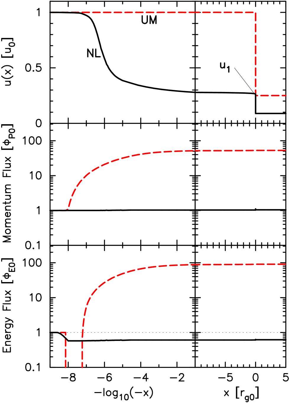
Figure 1.— The dashed (red) curves show the results for an unmodified shock with $R_{\mathrm{tot}}\simeq 4$ (Model UM). The solid (black) curves (Model A) show the self-consistent result where the momentum and energy fluxes are conserved across the shock. For this example, where all three instabilities are active, the self-consistent compression ratio is $R_{\mathrm{tot}}\simeq 11.3$ and $\sim 40$% of the energy flux is lost at the FEB at $x=-10^{8}\,r_{g0}$, where $r_{g0}\equiv m_{p}u_{0}c/(eB_{0})\simeq 5.6\!\times\!10^{-9}$ pc. Both models have $u_{0}=5000$ km s^-1, $n_{0}=0.3$ cm^-3, and $B_{0}=3$ $\mu$G. Note the split log–linear $x$-axis.

The momentum, $\Phi^{\mathrm{({\it i})MC}}_{P}(x)$, and energy, $\Phi^{\mathrm{({\it i})MC}}_{E}(x)$, fluxes from all particles are calculated directly in the Monte Carlo simulation for the $i$-th iteration. To these particle fluxes we add the wave components $P_{w}^{(i)}(x)$ and $F_{w}^{(i)}(x)$ and check to see if the total momentum and energy fluxes (i.e., equations 3 and 5) are conserved to within some limit at all $x$. If the fluxes are not conserved in the $i$-th iteration, we use equation (3) in the form

$$\rho_{0}u_{0}\,[u^{(i+1)}(x)-u^{(i)}(x)]+\Phi^{\mathrm{({\it i})MC}}_{P}(x)+P_{w}^{(i)}(x)=\Phi_{P0}\ ,$$ (60)

to predict the shock speed profile, $u^{(i+1)}(x)$, for the $i$-th$+1$ iteration.

When relativistic particles are produced and/or high-energy particles escape at an upstream FEB, the overall compression, $R_{\mathrm{tot}}$, will increase above $R_{\mathrm{RH}}$ and $R_{\mathrm{tot}}$ must be found by iteration simultaneously with $u(x)$ and $v_{\mathrm{scat}}(x)$. A consistent solution, within some statistical uncertainty, will conserve momentum and energy fluxes at all $x$, including a match to the escaping energy flux, $Q_{\mathrm{esc}}$ in equation (5). Despite the complexity of this system, with several processes all coupled nonlinearly, we are able to obtain unique modified shock solutions covering a wide dynamic range, with self-consistent injection, MFA, and an overall compression ratio consistent with particle escape.

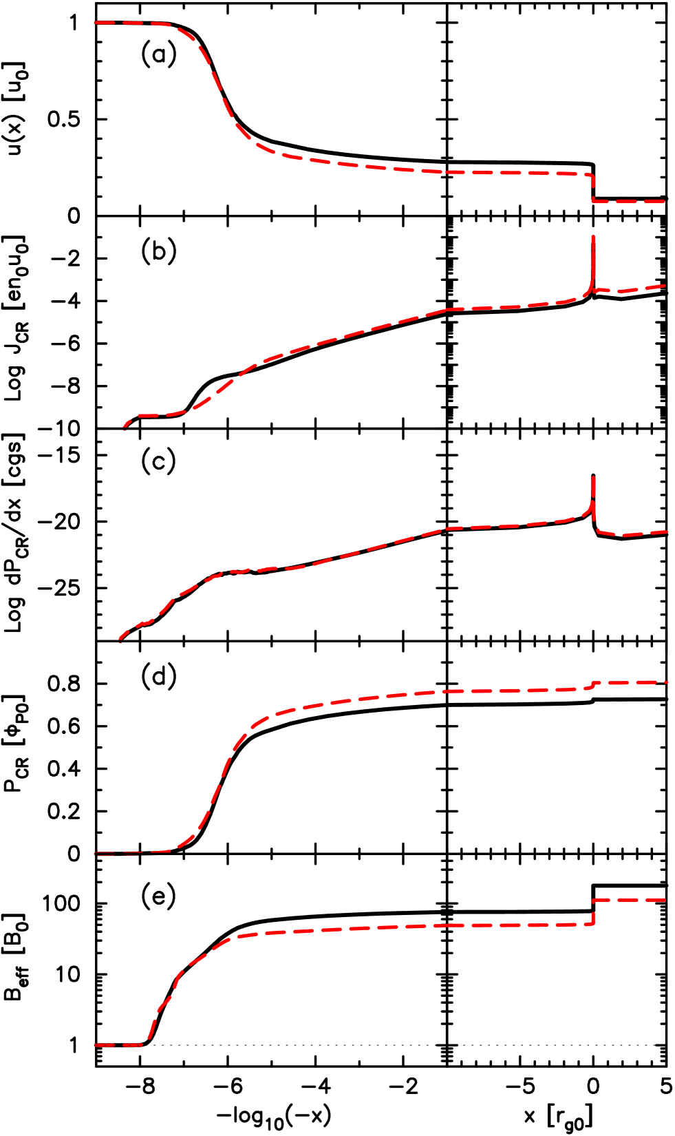
Figure 2.— The top panels (a) show the bulk flow speed as in Figure 1, panels (b) show the CR current, panels (c) show $dP_{\mathrm{cr}}/dx$ in cgs units, panels (d) show the CR pressure, and the bottom panels (e) show the effective magnetic field derived from equation (25). The dashed (red) curves include cascading (Model B) while the solid (black) curves (Model A) do not. Both models have $u_{0}=5000$ km s^-1, $n_{0}=0.3$ cm^-3, and $B_{0}=3$ $\mu$G.

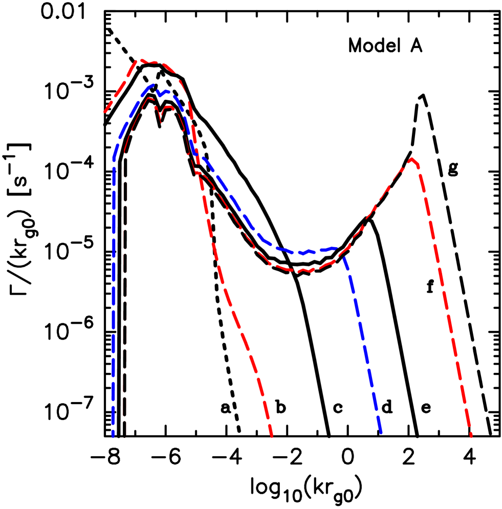
Figure 3.— The instability growth rate at different positions in the shock precursor for our nonlinear Model A. We plot $\Gamma/(kr_{g0})$ versus $kr_{g0}$ to reduce the scale spread and the labels indicate the $x$-positions where the curves are calculated: (a) $10^{8}$, (b) $10^{7}$, (c) $10^{6}$, (d) $1.9\!\times\!10^{3}$, (e) $5.2$, (f) $1.9\!\times\!10^{-3}$ and (g) $10^{-4}$, all in units of $-r_{g0}$. Compare this with Figure 1 in Bykov et al. (2011b).

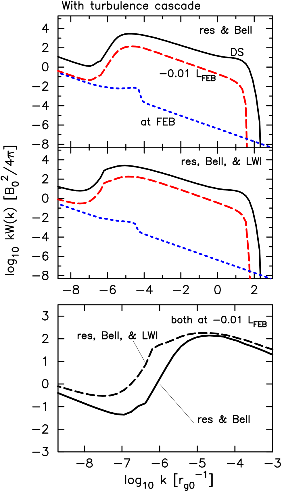
Figure 4.— Turbulence spectra for the example shown in Figure 2 with turbulence cascading. In the top two panels, the solid (black) curve is calculated downstream from the subshock, the dashed (red) curve is calculated in the shock precursor at $x=-0.01\,L_{\mathrm{FEB}}=-10^{6}r_{g0}$, and the dotted (blue) curve is calculated at the FEB. In the top panel (Model C), the LWI is not included while in the middle panel (Model A) it is. In all cases, the resonant instability is included. In the bottom panel, the cases with and without the LWI are compared at $x=-0.01\,L_{\mathrm{FEB}}$.

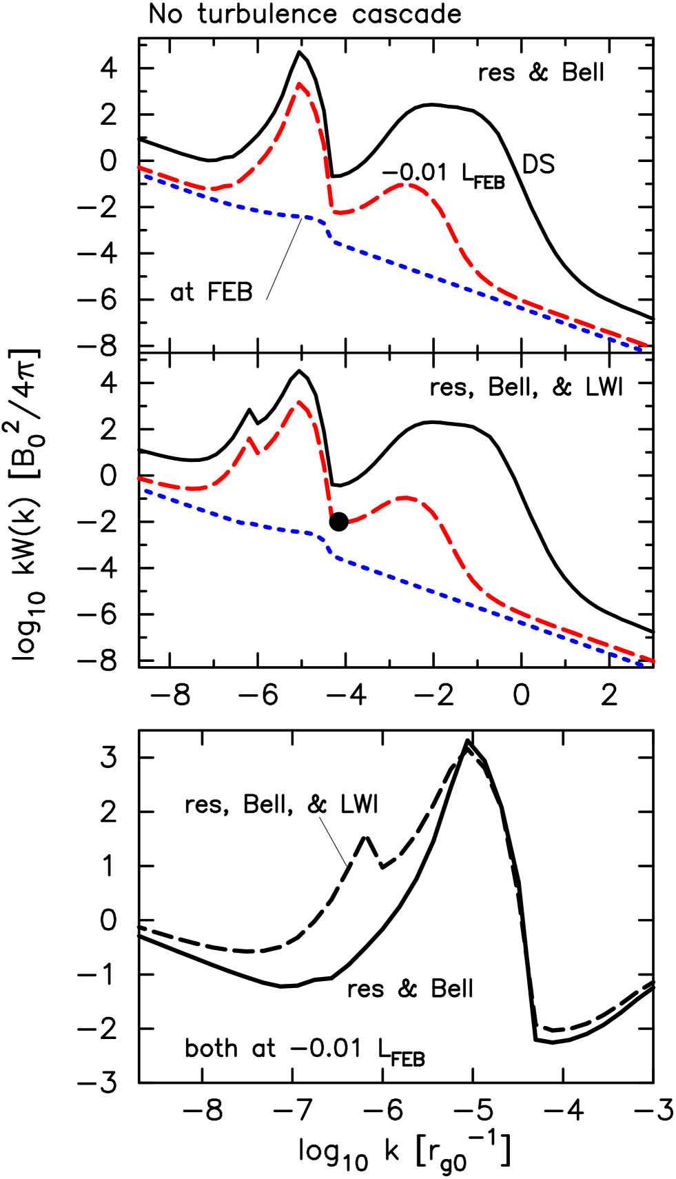
Figure 5.— Turbulence spectra for the example shown in Figure 2 without turbulence cascading. Other than cascading, all aspects of the figure are similar to Figure 4. The model without the LWI is Model D, while that with the LWI is Model A. The turbulence surrounding the solid dot in the middle panel corresponds roughly to the diffusion coefficient at the solid dot in the bottom panel of Figure 7.

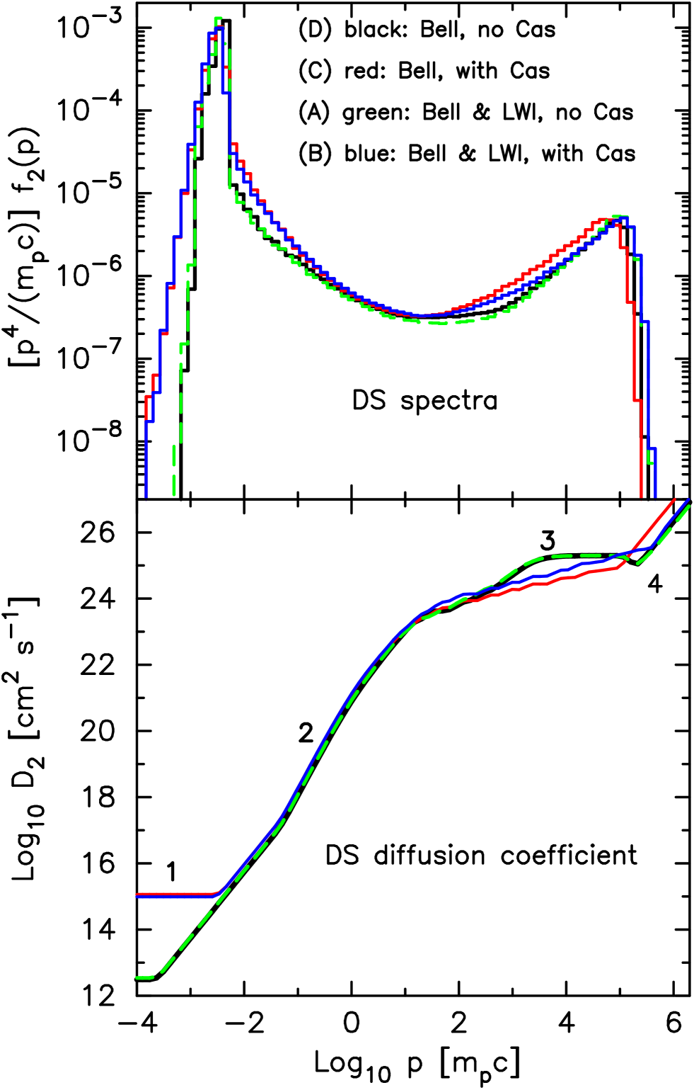
Figure 6.— Phase-space distributions, $[p^{4}/(m_{p}c)]f_{2}(p)$, and diffusion coefficients for the four examples shown in Figures 4 and 5 calculated downstream from the subshock. The color coding is the same for each panel and the labeled regions in the bottom panel are discussed in the text. Note that the resonant instability is active in all examples. Here and elsewhere the particle distribution is anisotropic and calculated in the shock frame and the plotted $f_{2}(p)$ is averaged over all angles and normalized such that $n(x)=4\pi\int_{0}^{\infty}f(x,p)p^{2}dp=n(x)$ is the local number density. The models are: black (D), red (C), green (A), and blue (B).

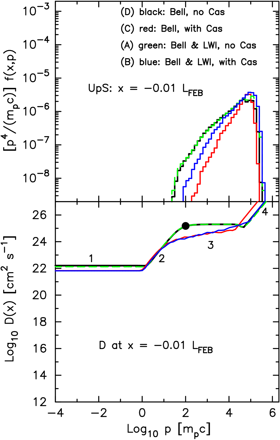
Figure 7.— Phase-space distributions, $[p^{4}/(m_{p}c)]f(x,p)$, and diffusion coefficients for the four examples shown in Figures 4 and 5 calculated in the shock precursor at $x=-0.01\,L_{\mathrm{FEB}}$. The color coding, labels, and normalization of $f(x,p)$ are the same as in Figure 6 and the resonant instability is active for all examples. The models are: black (D), red (C), green (A), and blue (B). Note that the cold incoming beam is present in the precursor but not shown in the upper panel. The solid dot in the bottom panel corresponds to the solid dot in the middle panel of Figure 5

Figure 8.— High momentum portion of the downstream phase-space distributions, $[p^{4}/(m_{p}c)]f_{2}(p)$, shown in Figure 6. The resonant instability is active for all examples. The models are: black (D), red (C), green (A), and blue (B).

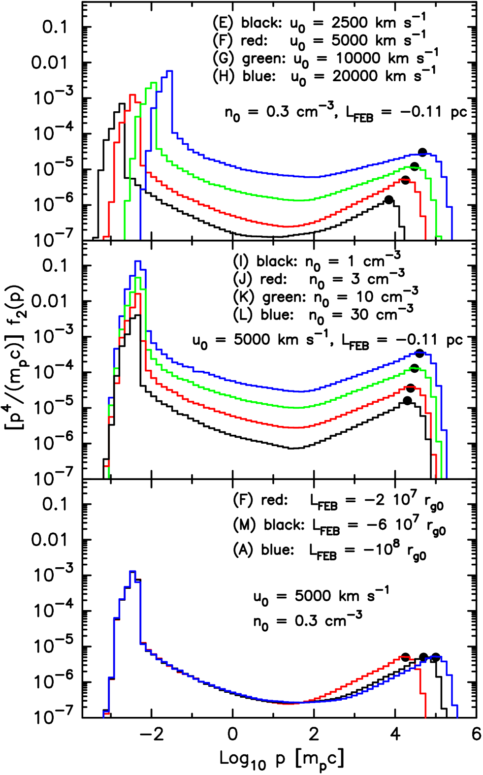
Figure 9.— Downstream, shock frame proton distribution functions calculated without cascading for the models as indicated. In the top panel, the shock speed, $u_{0}$, is varied, in the middle panel the ambient density, $n_{0}$, is varied, and in the bottom panel, the FEB, $L_{\mathrm{FEB}}$, is varied. Parameters held constant are shown in each panel. In all cases, $T_{0}=10^{4}$ K and $B_{0}=3$ $\mu$G. The solid dots indicate where $p^{4}f_{2}(p)$ is a maximum and defines $p_{\mathrm{max}}$.

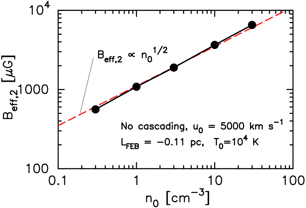
Figure 10.— The downstream amplified field, $B_{\mathrm{eff,2}}$, versus ambient density. The models running left to right are F, I, J, K, and L. The dashed (red) line shows the function as indicated.

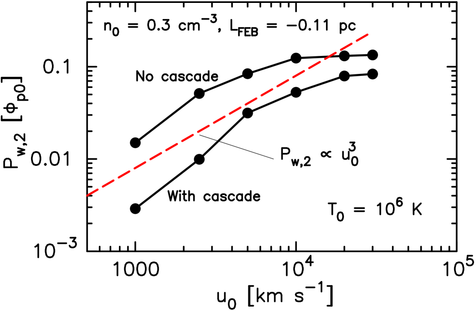
Figure 11.— Downstream pressure in turbulence versus shock speed for the models (running left to right) N, X, Y, Z, AA, and W without turbulence cascade and models Q, R, S, T, U, and V with cascade. The dashed (red) line approximates the behavior for low shock speeds.

Figure 12.— Comparison of our models (from left to right) N, X, Y, Z, AA, and W with equation (2) in Caprioli & Spitkovsky (2014). Note that $P_{\mathrm{cr}}^{\prime}=P_{\mathrm{cr}}/(\rho_{0}u_{0}^{2})$ plotted in the $y$-axis is the normalized CR pressure.

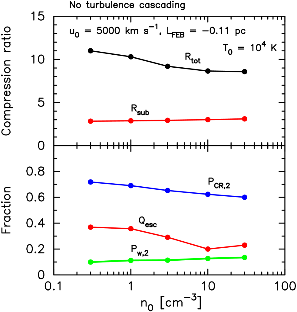
Figure 13.— The top panel shows the total and subshock compression ratios and the bottom panel shows the acceleration efficiency as given by the DS pressure in trapped CRs $P_{\mathrm{cr,2}}$, the DS pressure in turbulence $P_{w,2}$ (both as fractions of $\Phi_{P0}$), and the fraction of upstream energy flux escaping at the upstream FEB $Q_{\mathrm{esc}}$ versus ambient density for the models (from left to right) F, I, J, K, and L.

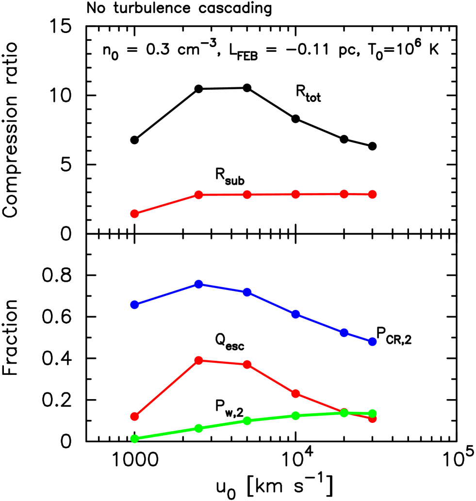
Figure 14.— The top panel shows the total and subshock compression ratios as a function of shock speed for fixed $n_{0}$ and physical distance to the FEB. In the bottom panel various quantities are shown as labeled. The CR and wave pressures are calculated downstream from the subshock as fractions of $\Phi_{P0}$ and $Q_{\mathrm{esc}}$ is given as the fraction of $\Phi_{E0}$. The models, running left to right, are N, X, Y, Z, AA, and W.

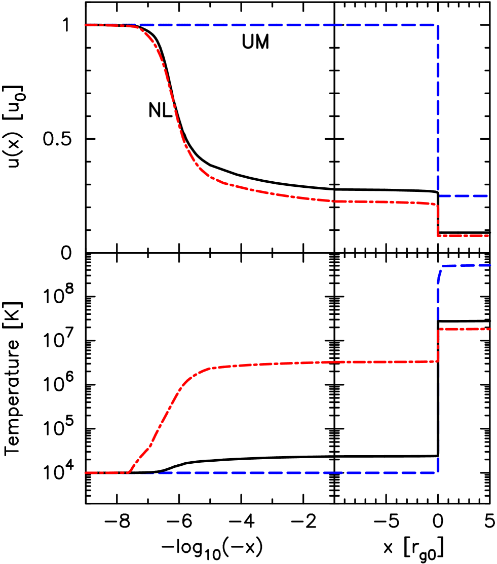
Figure 15.— The top panel compares the shock structure for an unmodified shock (model UM, dashed blue curve), a modified shock without cascading (model A, solid black curve), and a modified shock with cascading (model B, dot-dashed red curve) In the bottom panel, the temperature structure is shown using the same line notation.

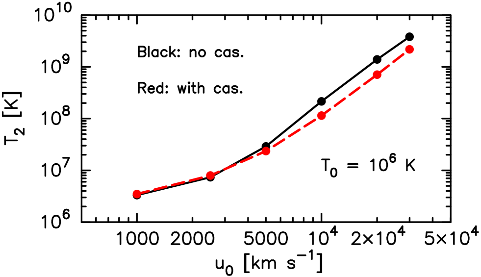
Figure 16.— Downstream temperatures with (dashed curve) and without (solid curve) cascading. The models without cascading, running left to right, are N, X, Y, Z, AA, and W. Those with cascading are Q, R, S, T, U, and V.

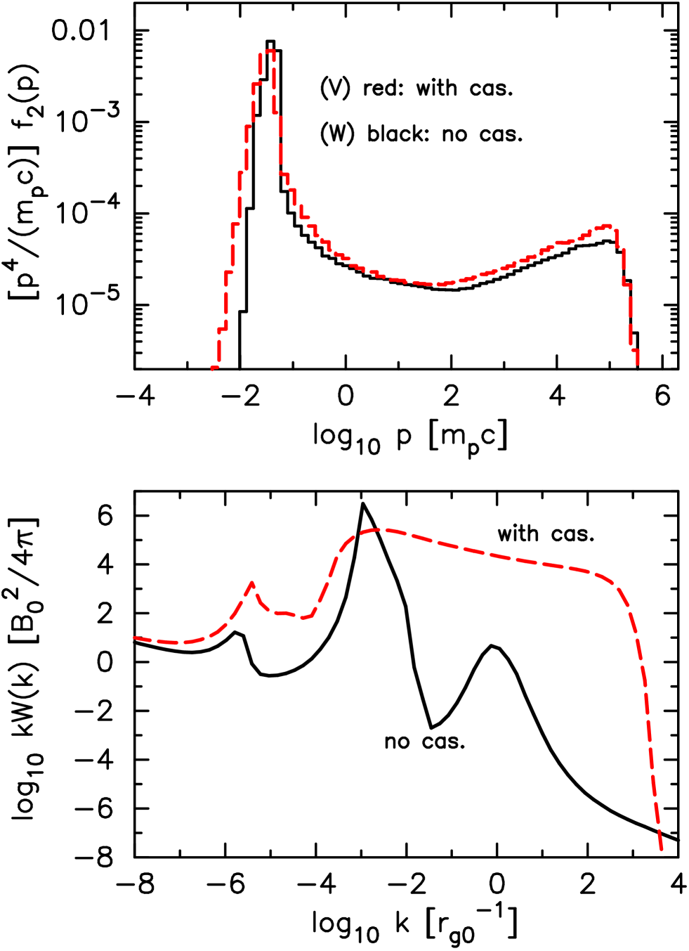
Figure 17.— The top panel shows the downstream phase-space distributions and the bottom panel shows the downstream turbulence for models W and V. These models have $u_{0}=3\!\times\!10^{4}$ km s^-1 and $L_{\mathrm{FEB}}\simeq 0.11$ pc.

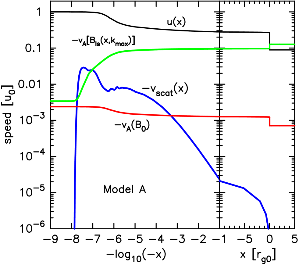
Figure 18.— The scattering center velocity $v_{\mathrm{scat}}(x)$ (blue line) derived from our Model A for a shock velocity $u_{0}=5\!\times\!10^{3}$ km s^-1, far upstream density $n_{0}=0.3$ cm^-3, far upstream magnetic field $B_{0}=3$ $\mu$G, and $L_{\mathrm{FEB}}\simeq 0.56$ pc. We also show the bulk flow velocity $u(x)$ (black line) and the Alfvén velocities calculated with the amplified magnetic field $B_{\mathrm{ls}}(x,k_{\mathrm{max}})$ (green line) and the initial field $B_{0}$ (red line). Note that $v_{\mathrm{scat}}$ and the Alfvén speeds are directed upwards so we plot the negative values.

3. Results

In our solutions, the bulk flow speed, $u(x)$, overall compression ratio, $R_{\mathrm{tot}}$, and CR induced magnetic turbulence are calculated such that the momentum and energy fluxes are conserved across the shock, as shown by the solid (black) curves in Figure 1 (model A in Table 1). These fluxes include the magnetic field contributions and account for the escaping energy flux at the FEB. The drop in energy flux seen in the solid curve at $x\sim-10^{8}\,r_{g0}$ in the bottom left panel of Figure 1 is a direct measure of the energy flux escaping at the FEB.

The dashed (red) curves in Figure 1 (model UM in Table 1) show the shock structure and fluxes for the same input parameters without shock smoothing, adjustment of $R_{\mathrm{tot}}$, or MFA. In the UM case, $R_{\mathrm{tot}}=R_{\mathrm{RH}}\simeq 4$, versus $R_{\mathrm{tot}}\simeq 11.3$ in the NL case, and the momentum and energy fluxes are $\sim 100$ times above the conserved values throughout much of the shock. These quantitative results, of course, depend on the efficiency of DSA which, in turn, depends on the details of our model, i.e., on the injection scheme, the MFA description, and the calculation of the scattering mean free path from the turbulence. Nevertheless, it is essential to note that any consistent description of efficient DSA with a diffusion coefficient that is an increasing function of momentum must produce a shock structure similar to the solid (black) curves shown in Figure 1.

In the self-consistent solution, the shock structure develops a distinct subshock with compression ratio $R_{\mathrm{sub}}<R_{\mathrm{tot}}$, as indicated by $u_{1}$ in the top panel of Figure 1. The subshock is responsible for most of the heating of the ambient material and in this case, $R_{\mathrm{sub}}=u_{1}/u_{2}\simeq 2.85$. In order to have a consistent solution with efficient DSA, the plasma heating must be reduced compared to the UM case, as reflected by $R_{\mathrm{sub}}<R_{\mathrm{tot}}$.

3.1. Magnetic Field Fluctuations Spectra

Our model gives a thorough accounting of the magnetic fluctuation amplification produced simultaneously by the three CR-current instabilities as discussed in §2.5. In Figure 2 we show the converged flow speed profile along with the CR current $J_{\mathrm{cr}}$, CR pressure gradient $dP_{\mathrm{cr}}/dx$, CR pressure $P_{\mathrm{cr}}$, and the effective magnetic field $B_{\mathrm{eff}}$ that results from MFA. Note that $B_{\mathrm{eff}}$ is obtained from equation (26) and does not include the homogeneous part of the ISM field. The dashed (red) curves (Model B in Table 1) include cascading while the solid (black) curves (Model A) do not. From the (d) and (e) panels it can be seen that cascading reduces the large-scale magnetic field by about a factor of two for $x\;\raise 1.29167pt\hbox{$>$\kern-7.5pt\raise-4.73611pt\hbox{$\sim$}}\;-10^{6}\,r_{g0}$ and causes the CR pressure to increase by $\sim 10\%$ over the same range. In both cases, the shock structure (panel a) adjusts so momentum and energy are conserved through the shock.

In Figure 3 we show $\Gamma(x,k)/(r_{g0})$ vs. $kr_{g0}$ as calculated from equation (20) for Model A. Here, $\Gamma(x,k)=2\,\mathrm{Im}[\omega(x,k)]$ is the growth rate of magnetic energy of the modes. The curves are calculated at different positions in the precursor going from the FEB at $x=-10^{8}r_{g0}$ (a) to just upstream of the subshock position at $x=10^{-4}r_{g0}$ (g). It is instructive to compare this figure with Figure 1 in Bykov et al. (2011b) where the growth rates for the three instabilities are plotted separately for a fixed set of parameters. In the Monte Carlo code, the combined turbulence growth rate is determined self-consistently from the three instabilities at each position in the shock precursor and the instantaneous growth rate varies widely as a function of position and wave number.

In addition to modifying the MFA, the efficiency of turbulence cascade through $k$-space strongly influences the spectrum of mesoscopic magnetic fluctuations. Unfortunately, the nature of turbulence cascade is not well understood. Local turbulence cascade parallel to the mean field can be suppressed in MHD turbulence (e.g., Goldreich & Sridhar, 1997; Biskamp, 2003; Sahraoui et al., 2006). We assume this to justify our models without cascade where we set $\Pi(x,k)=0$ in equation (7). Both the Bell and long-wavelength instabilities have maximum growth rates along the local mean magnetic field (e.g., Bykov et al., 2013a). We leave the more difficult issue of anisotropic cascading to future work.

In Figures 4 and 5 we show the turbulence, with and without cascading, calculated upstream at the FEB (dotted, blue curves), in the precursor at 1% of the distance to the FEB (dashed, red curves), and downstream from the shock (solid, black curves). As expected, cascading produces large differences in the turbulence at short wavelengths but the longest wavelengths are much less affected. Also shown in Figures 4 and 5 is the effect of the LWI. The top panels show the turbulence without the LWI ($N_{B}=0$), the middle panels show the case where resonant, Bell, and the LWI are combined, and the bottom panels show a long-wavelength comparison in the precursor at $x=-0.01\,L_{\mathrm{FEB}}$. The comparison at $x=-0.01\,L_{\mathrm{FEB}}$ in the bottom panels shows that the LWI broadens the spectral peak and shifts it toward larger scales. The LWI enhances the longest wavelength turbulence by at least an order of magnitude with or without cascading.

In the top panel of Figure 6 we show the shock frame, downstream proton phase-space distributions, multiplied by $p^{4}/(m_{p}c)$, for the four cases shown in Figures 4 and 5. The bottom panel shows the downstream diffusion coefficient, $D_{2}$, for these cases where $D_{2}$, or $\lambda(x,p)$, is determined from equation (52). Figure 7 is a similar plot calculated in the shock precursor at $x=-0.01\,L_{\mathrm{FEB}}=-10^{6}r_{g0}$. The regions indicated by numbers in Figures 6 and 7 have particular characteristics. The low momentum region 1 is where vortex convection dominates and $D_{2}$ is independent of $p$ (equation 45). For the upstream position shown in Figure 7, low-energy accelerated particles do not reach this position so there is no CR pressure gradient or current to produce turbulence on short scales. The highest energy region 4, is dominated by short-scale fluctuations (equation 48) and $D_{2}\propto p^{2}$. The intermediate range 2–3 is where quasi-resonant processes dominate and the $p$ dependence of $D_{2}$ depends on the interplay of $B_{\mathrm{ls}}$, $k$, and $W$ in equation (55). However, since $B_{\mathrm{ls}}$ depends on $W$ and $k$ through equation (19) there is no simple one-to-one correspondence between the turbulence shown in Figures 4 and 5 and $D_{2}$.

Nevertheless features such as the flattening of $D_{2}$ between regions 2 and 3 can be understood in general terms. In going from low to high $p$, the resonant $k$ decreases causing $B_{\mathrm{ls}}$ to decrease (equation 19). This, combined with the increase (or slow decrease) in $kW$ as $k$ decreases causes $\lambda(x,p)$ (equation 52) to increase slowly. Here, in region 3, $D_{2}$ increases less rapidly then $p$, i.e., slower than the Bohm limit. In contrast, in region 2, as $p$ increases, $k$ decreases, $kW$ flattens out and $D_{2}$ increases faster than $p^{2}$. The transition in $D_{2}$ from 2 to 3 indicated with a solid dot in the bottom panel of Figure 7 corresponds roughly to the turbulence at the position indicated by the solid dot in the middle panel of Figure 5.

While the magnetic fluctuation spectra with and without cascading are very different in the short-scale regime, as shown in Figures 4 and 5, the corresponding DS particle spectra, shown in Figure. 6, are quite similar. There is, however, a clear increase in $p_{\mathrm{max}}$ when the LWI operates with the Bell and resonant instabilities. This is shown in Figure 8, where $p_{\mathrm{max}}$ increases by about a factor of two when the LWI is included. This coupling between the short-wavelength modes from Bell’s instability (much shorter than the CR gyroradius) and the long-wavelength modes from the LWI (much longer than the CR gyroradius) highlights the need for simulations to cover a wide dynamic range in order to capture this essential physics.

3.2. Particle spectra

In Figure 9 we show downstream particle spectra where the resonant, Bell, and long-wavelength instabilities are active for shocks with varying speed (top panel), varying ambient density (middle panel), and varying $L_{\mathrm{FEB}}$ (bottom panel. For all plots there is no cascading, $T_{0}=10^{4}$ K, $B_{0}=3$ $\mu$G, the ISM turbulence is such that $B_{\mathrm{Kolm}}=3$ $\mu$G, and for the top two panels the FEB is at the same physical distance from the subshock, i.e., $L_{\mathrm{FEB}}\simeq-0.11$ pc.

In contrast to the top panel in Figure 6, where the downstream distribution functions vary little with changes in the turbulence generation and cascading, the spectra in Figure 9 vary importantly with $u_{0}$, $n_{0}$, and $L_{\mathrm{FEB}}$. For a given physical distance to the FEB (top panel), the maximum CR momentum, $p_{\mathrm{max}}$, increases with $u_{0}$. We indicate the trend in $p_{\mathrm{max}}$ with a solid dot placed at the maximum in $p^{4}f(p)$. This trend results from the fact that the upstream diffusion length scales as $1/u_{0}$ so a fixed $L_{\mathrm{FEB}}$ increases in terms of particle gyroradii as $u_{0}$ increases. The top panel also shows that the thermal peak and the minimum in the $p^{4}f(p)$ distribution increase with $u_{0}$. It is significant that the minimum in $p^{4}f(p)$ occurs well above $m_{p}c$ in all cases.

The middle and bottom panels of Figure 9 show that the normalization of $f_{2}(p$) scales as $n_{0}$ and $p_{\mathrm{max}}$ scales both with $L_{\mathrm{FEB}}$ and $n_{0}$. From the three sets of simulations in Figure 9 (and additional runs not shown for clarity), we obtain the scaling relation

$$p_{\mathrm{max}}\propto n^{\delta}_{0}\,u_{0}L_{\mathrm{FEB}}$$ (61)

or, assuming that $L_{\mathrm{FEB}}$ is some fraction of the shock radius $R_{\mathrm{sk}}$, one obtains $p_{\mathrm{max}}\propto n^{\delta}_{0}\,u_{0}R_{\mathrm{sk}}$. Notably, we find a rather weak dependence of $p_{\mathrm{max}}$ on $n_{0}$ of $\delta\sim$ 0.25 (middle panel of Figure 9). This result, for a quantity critical for all shock applications, is in contrast with the scaling expected if one assumes $D(p_{\mathrm{max}})/u_{0}\propto R_{\mathrm{sk}}$ and that $D(p_{\mathrm{max}})$ depends on the proton gyroradius $r_{g}(p_{\mathrm{max}})$ in the effective, downstream, amplified magnetic field, $B_{\mathrm{eff,2}}$. Since MFA depends on the ram pressure, it has been suggested that $B_{\mathrm{eff,2}}\propto\sqrt{n_{0}}\,u_{0}$ (see, e.g., Ptuskin et al., 2010; Schure & Bell, 2013b). In this case, $p_{\mathrm{max}}$ would scale as $\sqrt{n_{0}}\,u_{0}^{2}\,L_{\mathrm{FEB}}$, a stronger dependence on both the upstream density and the shock velocity then we find with our self-consistent simulations.

In regards to the postshock turbulent magnetic field, $B_{\mathrm{eff,2}}$, we find the following dependence on the far upstream density and shock velocity (see Figures 10 and 12)

$$B_{\mathrm{eff,2}}\propto\sqrt{n_{0}}u_{0}^{\theta}\ .$$ (62)

At $u_{0}\;\raise 1.29167pt\hbox{$>$\kern-7.5pt\raise-4.73611pt\hbox{$\sim$}}\;5,000$ km s^-1, the efficiency of MFA, defined as $P_{w,2}/\Phi_{P0}$, saturates at roughly 10-15% of the far upstream ram pressure (see Figure 11). This implies $P_{w,2}\propto u_{0}^{2}$, or $B_{\mathrm{eff,2}}^{2}\propto u_{0}^{2}n_{0}$, corresponding to $\theta\sim 1$. At lower shock velocities, we find $P_{w,2}/\Phi_{P0}\propto u_{0}$ (i.e., $P_{w,2}\propto u_{0}^{3}$), and therefore $B_{\mathrm{eff,2}}^{2}/n_{0}\propto u_{0}^{3}$, i.e., $\theta\sim$ 1.5. At shock velocities below $\sim 1000$ km s^-1, the efficiency of MFA drops to about a percent of the ram pressure.

In Figure 12 we compare our results with the scaling relation determined in Caprioli & Spitkovsky (2014) using hybrid simulations. Their equation (2) (with our notation) is

$$\left<\frac{B_{\mathrm{eff,2}}}{B_{0}}\right>^{2}_{\mathrm{sh}}\simeq 3\frac{P_{\mathrm{cr,2}}}{\Phi_{P0}}M_{A}\ ,$$ (63)

and it’s clear from Figure 12 that, while the Monte Carlo result matches equation (63) at $u_{0}=1000$ km s^-1 (i.e., $M_{A}=84$), it has a very different scaling at higher shock speeds and higher Alfvén Mach numbers. It is important to understand the reasons for this difference, which must stem from the different assumptions and parameters for the two simulations, since any modeling of a real object requires such scalings. Our Alfvén Mach numbers run from about 84 to 2500, whereas the hybrid results are for $M_{A}\;\raise 1.29167pt\hbox{$<$\kern-7.5pt\raise-4.73611pt\hbox{$\sim$}}\;100$. This is significant because MFA in shocks with Alfvén Mach numbers below about 30 is dominated by the resonant CR instability (e.g., Amato & Blasi, 2009b; Caprioli & Spitkovsky, 2014). In our high Mach number results, non-resonant instabilities dominate. Apart from different magnetizations, there are different assumptions made for the magnetic fluctuation spectra of the incoming plasma. In the Monte Carlo modeling, the initial spectrum of magnetic fluctuations is Kolmogorov, as determined by equation (59), whereas the initial fluctuations in the hybrid simulations are determined by numerical noise.

It is significant that the dependence of the post-shock turbulent magnetic field can be tested with SNR observations. The compilation by Vink (2012) (see his Figure 39) can be understood if the scaling $P_{w,2}\propto u_{0}^{3}$ (i.e., $B_{\mathrm{eff,2}}^{2}\propto u_{0}^{3}n_{0}$) holds at shock velocities below $\sim 10^{4}$ km s^-1 and changes to $P_{w,2}\propto u_{0}^{2}$ (i.e., $B_{\mathrm{eff,2}}^{2}\propto u_{0}^{2}n_{0}$) at higher shock velocities. We find that this scaling holds for both upstream temperatures $T_{0}=10^{4}$ and $10^{6}$ K, indicating that it is not a sonic Mach number effect, at least for fairly large $M_{S}$. We also find that it is only weakly dependent on the far upstream mean field $B_{0}$, indicating only a weak Alfvén Mach number dependence. In addition, the scaling doesn’t depend strongly on $L_{\mathrm{FEB}}$.

Apart from the magnetic field–shock velocity scalings, high spatial resolution Chandra X-ray observations of Tycho’s SNR reported by Eriksen et al. (2011) have revealed coherent synchrotron structures which may be related to amplified magnetic fields (e.g., Bykov et al., 2011a; Malkov et al., 2012b). The presence of long-wavelength peaks in magnetic turbulence spectra, which are apparent in Figures 5 and 17 (bottom panel), may be tested with high resolution synchrotron images. We shall discuss the modeling of synchrotron images elsewhere.

Other scalings include the acceleration efficiency, as indicated by the escaping CR energy flux $Q_{\mathrm{esc}}$, the DS CR pressure $P_{\mathrm{cr,2}}$, the DS wave pressure $P_{w,2}$, and the shock compression ratios, $R_{\mathrm{tot}}$ and $R_{\mathrm{sub}}$. In Figures 13 and 14 we show these scalings for shocks without cascading and for $L_{\mathrm{FEB}}\simeq-0.11$ pc. We find that increasing $n_{0}$ from 0.3 to 30 cm^-3 (Figure 13) results in a decrease of $R_{\mathrm{tot}}$ from $\sim 11$ to $\sim 8.6$ with a corresponding increase in $R_{\mathrm{sub}}$ from $\sim 2.8$ to $\sim 3.1$. In Figure 14 we see that as $u_{0}$ and the shock strength increase, $R_{\mathrm{tot}}$ and $Q_{\mathrm{esc}}$ first increase and then decrease. Since $L_{\mathrm{FEB}}$ is set at a fixed physical distance for these examples, the size of the shock acceleration site decreases with increasing $u_{0}$ resulting in a lower $p_{\mathrm{max}}$, as shown in the top panel of Figure 9. The decrease in $p_{\mathrm{max}}$ dominates the increase in shock strength causing $Q_{\mathrm{esc}}$ to decrease when $u_{0}\;\raise 1.29167pt\hbox{$>$\kern-7.5pt\raise-4.73611pt\hbox{$\sim$}}\;2500$ km s^-1.

3.2.1 Cascading and Thermodynamic Properties

In Figure 15 we show the effects of cascading and the smooth shock structure on the background plasma temperature. The dashed (blue) curves are for an unmodified shock (Model UM), the solid (black) curves are for a modified shock without cascading (Model A), and the dot-dashed (red) curves are for a modified shock with cascading (Model B). As in Vladimirov et al. (2009), without cascading the dissipation term, $L$, in equation (7) is set to zero. When cascading is included, we assume viscous dissipation such that ${\cal L}=v_{a}k^{2}k_{d}^{-1}W$ (e.g., Vainshtein et al., 1993). The wavenumber, $k_{d}$, is identified with the inverse of the thermal proton gyroradius: $k_{d}(x)=eB_{\mathrm{ls}}(x,k_{d})/[c\sqrt{m_{p}k_{B}T(x)}]$, where $T(x)$ is the local gas temperature determined from the heating induced by $L$, as described in Vladimirov et al. (2008).

Without cascading, or in the UM shock, the precursor temperature remains within a factor of 3 of $T_{0}$ until a sharp increase occurs at the subshock. In contrast, cascading heats the precursor substantially so $T(x)\;\raise 1.29167pt\hbox{$>$\kern-7.5pt\raise-4.73611pt\hbox{$\sim$}}\;100T_{0}$ well in front of the subshock which may produce observable consequences. The downstream temperature is dramatically reduced in the nonlinear cases compared to the UM shock and $T_{2}$ is slightly less with cascading than without.

In Figure 16 we compare the downstream temperature for a different set of shocks with and without turbulence cascading as a function of $u_{0}$. It’s clear that $T_{2}$ is not very sensitive to cascading despite the large effect on the precursor temperature, although the difference is larger for larger $u_{0}$. In the top panel of Figure 17, we show DS proton spectra for $u_{0}=3\!\times\!10^{4}$ km s^-1. The fluxes at the high-energy end of the spectra are somewhat sensitive to the turbulent cascading, while the maximum proton energy is not. As we have emphasized earlier, nonlinear effects damp changes that might otherwise be expected from the large differences in the self-generated turbulence (bottom panel). If the acceleration is as efficient as we show here, conservation considerations force the shock to adjust such that the particle distribution functions cannot vary substantially. In contrast to the turbulence for the $u_{0}=5\!\times\!10^{3}$ km s^-1 shock shown in Figure 4, the spectrum with cascading for $u_{0}=3\!\times\!10^{4}$ km s^-1 shows a clear long-wavelength peak (dashed red curve in the bottom panel of Figure 17).

3.3. Scattering Center Velocity

As described in Section 2.6, we calculate the scattering center velocity, $v_{\mathrm{scat}}(x)$, from conservation considerations without assuming any specific form for the turbulence, in particular, without assuming Alfvén waves. This macroscopic approach guarantees that the energy in the growing magnetic turbulence, which produces the CR scattering, is taken from the free energy of the anisotropic CR distribution.

In contrast, if the scattering center velocity is calculated in a microscopic, quasi-linear approach, one has to weight the phase velocities of the modes with the anisotropy of their wave-vector distributions. In the simplest case of the resonant CR streaming instability, the amplified modes are assumed to be Alfvén modes with wave-vectors aligned against the CR pressure gradient in the shock precursor. The situation is much more complicated for the dominant Bell and long wavelength nonresonant instabilities. For these, no simple Alfvén-wave-like assumption is adequate.

In Figure 18 we show $v_{\mathrm{scat}}(x)$ from Model A along with the mean flow speed, $u(x)$, and the Alfvén speeds derived with the upstream field $B_{0}$ and with the local amplified field $B_{\mathrm{ls}}(x,k_{\mathrm{max}})$. It is seen that $v_{\mathrm{scat}}(x)$ is everywhere well below $u(x)$ so there is no sizeable CR spectral softening due to a finite scattering center velocity. The Monte Carlo $v_{\mathrm{scat}}(x)$ exceeds the Alfvén speed calculated with $B_{0}$ in most of the precursor, but is well below the Alfvén speed determined by the amplified $B_{\mathrm{ls}}(x,k_{\mathrm{max}})$ except in the far upstream region near the FEB. If $v_{a}[B_{\mathrm{ls}}(x,k_{\mathrm{max}})]$ gives the scattering center speed, strong MFA implies significant softening of the CR spectrum since the effective compression ratio for DSA will be less than $R_{\mathrm{tot}}$. Such softening has been discussed by Zirakashvili & Ptuskin (2008), Blasi (2013), and Kang et al. (2013).

Morlino & Caprioli (2012) have suggested that a large scattering speed resulting from MFA and rapid Alfvén waves in DSA with CR acceleration efficiencies $\simeq 20$%, could produce CR spectra steeper than $dN/dE\propto E^{-2}$. If so, this might address the issue of the steep CR spectrum derived from Fermi observations of Tycho’s SNR (see also Caprioli, 2012; Slane et al., 2014). However, in general, the situation is not this simple.

Zirakashvili et al. (2013) recently showed that to explain the available multi-wavelength observations of Cas A, nonlinear DSA (with a total efficiency  $>$$\sim$  25%) of electrons, protons, and oxygen ions, by both the forward and reverse shocks, must be invoked. Particle injection in their kinetic models is an adjustable parameter and was varied independently for the forward and reverse shocks to fit the multi-wavelength observations. The model results in a variety of spectral shapes – hard spectra for oxygen ions accelerated in the reverse shock and soft for proton spectra from the forward shock with spectral indexes above 2, as inferred for Tycho. Furthermore, soft CR spectra might be expected for quasi-perpendicular shocks where the angle between the shock normal and the ambient magnetic field $\sim 90^{\circ}$ (e.g., Schure & Bell, 2013b). Another uncertainty occurs for DSA in partially ionized plasmas where the shock compression is reduced by the neutral return flux (e.g., Blasi et al., 2012; Blasi, 2013). We cite these cases to emphasize that the interpretation of gamma-ray emission from DSA in young SNRs requires careful modeling of complicated systems and is not yet fully developed.

4. Discussion and Conclusions

We have presented a comprehensive, nonlinear model of magnetic field amplification in shocks undergoing DSA. The magnetic turbulence responsible for scattering particles is calculated self-consistently from the free energy in the anisotropic, position dependent, distributions of those particles. For the first time, we simultaneously include turbulence growth from the resonant CR streaming instability together with the non-resonant short– and long–wavelength, CR–current–driven instabilities. From the magnetic turbulence, we determine the particle diffusion coefficient with a set of assumptions that depend on the particle momentum. Our plane-parallel, steady-state model includes shock modification and thermal particle injection and, for the parameters assumed here, results in efficient acceleration with $Q_{\mathrm{esc}}$ up to $\sim 50\%$ of the incoming energy flux and large downstream CR pressures. We have explored the implications of this efficient acceleration with a limited parameter survey.

Despite the approximations required, we believe this is the most general description of NL DSA yet presented for the following reasons:
(1) The Monte Carlo technique has a wide dynamic range and can follow particles from injection at thermal energies ($\sim 1$ eV) to escape at PeV energies. This range is currently far greater than can be achieved with PIC simulations or hydrodynamic turbulence calculations. Since no assumption of near-isotropy is required, both the injection of thermal particles and the escape of the highest energy CRs can be treated self-consistently with a determination of the shock structure. Modeling the feedback between thermal and PeV particles is essential in high Mach number shocks typical of young SNRs since CRs near $p_{\mathrm{max}}$ can contain a large fraction of the shock ram kinetic energy;
(2) Our iterative model is the first to include the combined growth rates for resonant and non-resonant CR-driven instabilities and to derive these from the highly anisotropic CR distributions in the self-consistently determined shock precursor. The instabilities produce highly amplified magnetic fluctuations which feed on one another making a consistent treatment essential;
(3) The iterative technique also provides a way to calculate the scattering center speed $v_{\mathrm{scat}}(x)$, directly from energy conservation without assuming any particular form for the magnetic turbulence. This approach is different from all previous treatments of the effects of a finite scattering center speed on DSA. Since the CR current modifies the dispersion properties of the magnetic modes and results in fast non-resonant instabilities in the shock precursor, there is no reason to assume the self-generated turbulence in NL shocks is well described as Alfvén waves. We do not assume this and believe ours is the first attempt at a general determination of $v_{\mathrm{scat}}$ since the resonant Alfvén wave instability was introduced for NL DSA by McKenzie & Voelk (1982).

Other non-test-particle techniques that are currently being used to study NL DSA and MFA with instabilities in addition to the resonant streaming instability are MHD calculations or plasma simulations, either full-particle PIC or hybrid.

Three-dimensional MHD calculations have been performed by Bell et al. (2013) (see also Bell et al., 2011; Schure & Bell, 2013a, and references therein) where the CRs are modeled kinetically and the CR current responsible for the non-resonant hybrid (NRH) (i.e., Bell) instability is included self-consistently. Particular attention is given to the escaping CRs in this work and, based on estimates for the escaping CR current needed to produce enough NRH turbulence to confine high-energy CRs, the model predicts the maximum CR energy without scaling by the age or size of the accelerator (see, for example, Blasi et al., 2007b, for earlier work on determining $p_{\mathrm{max}}$ taking into account nonlinear effects). Due to the computational requirements of the 3D MHD simulation, however, the CR momentum range is restricted to a factor of order 10–100 and large shock speeds ($c/5$) are assumed.

As is well known, plasma simulations have a great advantage over other techniques because, in principle, they provide a full, self-consistent calculation of the shock formation, particle injection and acceleration, and magnetic turbulence generation. This comes with severe computational requirements imposed by directly following particles in a self-generated magnetic field where the relevant length and time scales are set by the mircoscopic plasma parameters. For a hybrid simulation, the basic length scale is the ion inertial length, $c/\omega_{\mathrm{pi}}$, and the basic time scale is the ion gyro-period $t_{g}=m_{p}c/(eB_{0})$.

Recently, Caprioli & Spitkovsky (2014) (see also Caprioli & Spitkovsky, 2013a, b) have presented hybrid simulations of large, high Mach number, parallel shocks. They see some evidence for the LWI and suggest this may be from escaping CRs. As we noted in our discussion of Figure 12, however, we see a very different MFA scaling from their equation (2). While it is not clear what causes this, the basic assumptions and scales of the two simulations are extremely different. For the time-dependent PIC simulations of Caprioli & Spitkovsky (2014), for a background field $B_{0}=3$ $\mu$G, the largest dimension in a two-dimensional box was $L_{\mathrm{max}}=4\!\times\!10^{5}c/\omega_{\mathrm{pi}}\simeq 5\!\times\!10^{-6}$ pc, the longest run time was $t_{\mathrm{max}}=2500t_{g}\simeq 3\!\times\!10^{-3}$ yr, and the momentum range was less than three decades. For the run with $L_{\mathrm{max}}=4\!\times\!10^{5}c/\omega_{\mathrm{pi}}$, the transverse size was $1000\,\omega_{\mathrm{pi}}\simeq 10^{-8}$ pc. In comparison, the steady-state Monte Carlo shocks used to generate Figure 12 had $L_{\mathrm{FEB}}\simeq 0.11$ pc, followed CR acceleration for the equivalent of 100’s of years, and had a momentum range of $\sim 8$ decades. Regardless of the computational limits of the plasma simulations, they contain critical plasma physics that is not modeled with the Monte Carlo or MHD techniques making it important to meaningfully match the “small-scale” plasma simulation results to the “large-scale” Monte Carlo results to obtain a consistent calculation over a dynamic range large enough in both space and time to model SNRs.

The results we have presented are all for highly efficient DSA since our main goal is to study the effects of MFA from the three CR-driven instabilities in such cases. While global CR acceleration efficiencies on the order of $\simeq 10\%$ are generally assumed for SNRs, and efficiencies on this order are obtained by simpler parameterized NL models (e.g., Ellison et al., 2012), local efficiencies could be far higher (e.g., Völk et al., 2003). There is also indirect evidence from multi-wavelength observations of some SNRs for high efficiencies (see, for example, Hughes et al., 2000; Reynolds, 2008; Helder et al., 2012). We note that a direct observation of CR acceleration efficiency $\simeq 25\%$ was obtained at the small, weak quasi-parallel Earth bow shock (Ellison et al., 1990b) and we see no fundamental reason, either from theory or SNR observations, that restricts the intrinsic acceleration efficiency to values well below what we model at large, strong, SNR shocks, at least in some circumstances.

The efficiency of DSA, at least in terms of the downstream $P_{\mathrm{cr}}$, is potentially observable through the widths of Balmer lines from young SNRs in partially ionized material. This gives an estimate of the electron temperature and a model dependent estimate of the ion temperature and CR pressure can be obtained in association with X-ray observations and a measurement of the shock velocity. We note that neutrals may play an important role in the energy balance of shocks with velocities below $\sim 3000$ km s^-1  propagating in partially ionized media (see Helder et al., 2012; Blasi, 2013; Bykov et al., 2013c, for reviews). Here, we assumed fully ionized plasmas and did not attempt to model the effects of neutrals. To directly compare the pressure in the trapped downstream CR particles with that derived from Balmer line observations, one should account for the effects of neutrals and the realistic geometry of the postshock flow in a nonlinear DSA model.

Of course the spectral shape is an additional fundamental prediction of DSA and concave spectra as hard as we show may present a problem in this regard, as mentioned above in our discussion of $v_{\mathrm{scat}}$. We caution that, as is generally the case, we make a diffusion approximation for CR propagation. However, Bell et al. (2011) showed that diffusive propagation may break down for CRs in oblique shocks. They found that higher order anisotropies, that appear in a non-diffusion model, may result in harder spectra at quasi-parallel shocks and softer spectra at quasi-perpendicular shocks. It is important to point out that departures from standard diffusive propagation may be important in nonlinear shocks and such propagation may modify the spectral shape. We shall consider such departures in a seperate paper.

Table 1Model Parameters.^†

Model	Inst.	$u_{0}$	$n_{0}$	$L_{\mathrm{FEB}}$	$M_{S}:M_{A}$	$R_{\mathrm{tot}}$:$R_{\mathrm{sub}}$	$P_{\mathrm{cr,2}}$	$P_{w,2}$	$Q_{\mathrm{esc}}$	$B_{\mathrm{eff,2}}$	$T_{2}$
		km s-1	cm-3	pc			%	%	%	$\mu$G	$10^{6}$ K
UM	…	5000	0.3	0.56	$430:420$	$4.0:4.0$	…	…	…	3	490
A	B, L	5000	0.3	0.56	$430:420$	$11.3:2.85$	73	9	37	540	30
B	B, L, C	5000	0.3	0.56	$430:420$	$13.3:2.52$	80	3.5	47	330	20
C	B, C	5000	0.3	0.56	$430:420$	$12.5:2.37$	79	3.5	42	340	20
D	B	5000	0.3	0.56	$430:420$	$10.2:2.84$	69	10	35	570	35
E	B, L	2500	0.3	0.11	$210:210$	$11.7:2.81$	76	6	41	220	6
F	B, L	5000	0.3	0.11	$430:420$	$11.0:2.83$	72	10	37	560	30
G	B, L	10000	0.3	0.11	$850:840$	$8.3:2.85$	61	12	23	1250	220
H	B, L	20000	0.3	0.11	$1700:1670$	$6.93:2.87$	52	14	15	2600	1400
I	B, L	5000	1	0.11	$430:760$	$10.3:2.88$	69	11	36	1100	35
J	B, L	5000	3	0.11	$430:1300$	$9.2:2.92$	65	11	29	1900	45
K	B, L	5000	10	0.11	$430:2400$	$8.65:3.01$	62	13	25	3700	50
L	B, L	5000	30	0.11	$430:4200$	$8.58:3.10$	60	14	23	6500	55
M	B, L	5000	0.3	0.34	$430:420$	$11.0:2.83$	72	9	39	520	30
N	B, L	1000	0.3	0.11	$8.5:84$	$6.78:1.45$	66	1.5	12	41	3.3
P	B, L	30000	0.3	0.11	$2560:2500$	$6.33:2.85$	48	13	11	3900	3800
Q	B,L,C	1000	0.3	0.11	$8.5:84$	$6.72:1.33$	66	0.3	19	19	3.5
R	B,L,C	2500	0.3	0.11	$21:210$	$10.4:1.94$	75	1.0	31	90	7.9
S	B,L,C	5000	0.3	0.11	$43:420$	$11.9:2.16$	79	3	44	315	24
T	B,L,C	10000	0.3	0.11	$85:840$	$10.9:2.34$	75	5.3	39	820	110
U	B,L,C	20000	0.3	0.11	$170:1700$	$9.15:2.43$	68	8	28	2000	710
V	B,L,C	30000	0.3	0.11	$260:2500$	$8.0:2.47$	63	8.5	23	3100	2200
W	B,L	30000	0.3	0.11	$260:2500$	$6.33:2.85$	48	13	11	3900	3800
X	B,L	2500	0.3	0.11	$21:210$	$10.5:2.13$	75	5	39	200	7.3
Y	B,L	5000	0.3	0.11	$43:420$	$10.5:2.6$	72	8.4	37	520	29
Z	B,L	10000	0.3	0.11	$85:840$	$8.31:2.79$	61	12.4	23	1250	215
AA	B,L	20000	0.3	0.11	$170:1700$	$6.84:2.83$	52	13	14	2600	1400

^†For all models, $B_{0}=B_{\mathrm{Kolm}}=3\!\times\!10^{-6}$ G and we note that the derived results for all runs have a statistical uncertainty of $\;\raise 1.29167pt\hbox{$<$\kern-7.5pt\raise-4.73611pt\hbox{$\sim$}}\;5\%$.

References

- Achterberg (1981) Achterberg, A. 1981, Astronomy and Astrophysics, 98, 161
- Amato & Blasi (2006) Amato, E. & Blasi, P. 2006, MNRAS, 371, 1251
- Amato & Blasi (2009a) Amato, E. & Blasi, P. 2009a, MNRAS, 392, 1591
- Amato & Blasi (2009b) Amato, E. & Blasi, P. 2009b, MNRAS, 392, 1591
- Baring et al. (1997) Baring, M. G., Ogilvie, K. W., Ellison, D. C., & Forsyth, R. J. 1997, Astrophysical Journal, 476, 889
- Bell (1978) Bell, A. R. 1978, MNRAS, 182, 147
- Bell (2004) Bell, A. R. 2004, MNRAS, 353, 550
- Bell (2005) Bell, A. R. 2005, MNRAS, 358, 181
- Bell et al. (2011) Bell, A. R., Schure, K. M., & Reville, B. 2011, MNRAS, 418, 1208
- Bell et al. (2013) Bell, A. R., Schure, K. M., Reville, B., & Giacinti, G. 2013, MNRAS, 431, 415
- Berezhko & Ellison (1999) Berezhko, E. G. & Ellison, D. C. 1999, ApJ, 526, 385
- Berezhko & Krymskiĭ (1988) Berezhko, E. G. & Krymskiĭ, G. F. 1988, Soviet Physics Uspekhi, 31, 27
- Biskamp (2003) Biskamp, D. 2003, Magnetohydrodynamic Turbulence
- Blandford & Eichler (1987) Blandford, R. & Eichler, D. 1987, Physics Reports, 154, 1
- Blandford & Funk (2007) Blandford, R. & Funk, S. 2007, in American Institute of Physics Conference Series, Vol. 921, The First GLAST Symposium, ed. S. Ritz, P. Michelson, & C. A. Meegan, 62–64
- Blasi (2013) Blasi, P. 2013, A&A Rev., 21, 70
- Blasi et al. (2007a) Blasi, P., Amato, E., & Caprioli, D. 2007a, MNRAS, 375, 1471
- Blasi et al. (2007b) Blasi, P., Amato, E., & Caprioli, D. 2007b, MNRAS, 375, 1471
- Blasi et al. (2012) Blasi, P., Morlino, G., Bandiera, R., Amato, E., & Caprioli, D. 2012, Astrophysical Journal, 755, 121
- Burgess & Scholer (2013) Burgess, D. & Scholer, M. 2013, Space Sci. Rev., 178, 513
- Bykov (1982) Bykov, A. M. 1982, Soviet Astronomy Letters, 8, 320
- Bykov et al. (2013a) Bykov, A. M., Brandenburg, A., Malkov, M. A., & Osipov, S. M. 2013a, Space Sci. Rev., 178, 201
- Bykov et al. (2011a) Bykov, A. M., Ellison, D. C., Osipov, S. M., Pavlov, G. G., & Uvarov, Y. A. 2011a, The Astrophysical Journal Letters, 735, L40
- Bykov et al. (2012) Bykov, A. M., Ellison, D. C., & Renaud, M. 2012, Space Sci. Rev., 166, 71
- Bykov et al. (2013b) Bykov, A. M., Gladilin, P. E., & Osipov, S. M. 2013b, MNRAS, 429, 2755
- Bykov et al. (2013c) Bykov, A. M., Malkov, M. A., Raymond, J. C., Krassilchtchikov, A. M., & Vladimirov, A. E. 2013c, Space Sci. Rev., 178, 599
- Bykov et al. (2011b) Bykov, A. M., Osipov, S. M., & Ellison, D. C. 2011b, MNRAS, 410, 39
- Bykov & Toptygin (1993) Bykov, A. M. & Toptygin, I. N. 1993, Physics-Uspekhi, 36, 1020
- Caprioli (2012) Caprioli, D. 2012, J. Cosmology Astroparticle Physics, 7, 38
- Caprioli et al. (2010) Caprioli, D., Amato, E., & Blasi, P. 2010, Astroparticle Physics, 33, 307
- Caprioli & Spitkovsky (2013a) Caprioli, D. & Spitkovsky, A. 2013a, The Astrophysical Journal Letters, 765, L20
- Caprioli & Spitkovsky (2013b) Caprioli, D. & Spitkovsky, A. 2013b, ArXiv e-prints
- Caprioli & Spitkovsky (2014) Caprioli, D. & Spitkovsky, A. 2014, ArXiv e-prints
- Casse et al. (2002) Casse, F., Lemoine, M., & Pelletier, G. 2002, Phys. Rev. D, 65, 023002
- Drury (2011) Drury, L. O. 2011, MNRAS, 415, 1807
- Drury & Falle (1986) Drury, L. O. & Falle, S. A. E. G. 1986, MNRAS, 223, 353
- Ellison et al. (1996) Ellison, D. C., Baring, M. G., & Jones, F. C. 1996, Astrophysical Journal, 473, 1029
- Ellison & Bykov (2011) Ellison, D. C. & Bykov, A. M. 2011, Astrophysical Journal, 731, 87
- Ellison et al. (1993) Ellison, D. C., Giacalone, J., Burgess, D., & Schwartz, S. J. 1993, J. Geophys. Res., 98, 21085
- Ellison et al. (1981) Ellison, D. C., Jones, F. C., & Eichler, D. 1981, J. Geophys. (Zeitschrift Geophysik), 50, 110
- Ellison et al. (1990a) Ellison, D. C., Jones, F. C., & Reynolds, S. P. 1990a, Astrophysical Journal, 360, 702
- Ellison et al. (1990b) Ellison, D. C., Moebius, E., & Paschmann, G. 1990b, Astrophysical Journal, 352, 376
- Ellison et al. (2012) Ellison, D. C., Slane, P., Patnaude, D. J., & Bykov, A. M. 2012, Astrophysical Journal, 744, 39
- Ellison et al. (2013) Ellison, D. C., Warren, D. C., & Bykov, A. M. 2013, Astrophysical Journal, 776, 46
- Eriksen et al. (2011) Eriksen, K. A., Hughes, J. P., Badenes, C., et al. 2011, Astrophysical Journal, 728, L28+
- Ferrand et al. (2012) Ferrand, G., Decourchelle, A., & Safi-Harb, S. 2012, Astrophysical Journal, 760, 34
- Gargaté & Spitkovsky (2012) Gargaté, L. & Spitkovsky, A. 2012, Astrophysical Journal, 744, 67
- Giacalone et al. (1997) Giacalone, J., Burgess, D., Schwartz, S. J., Ellison, D. C., & Bennett, L. 1997, J. Geophys. Res., 102, 19789
- Giacalone & Jokipii (2007) Giacalone, J. & Jokipii, J. R. 2007, The Astrophysical Journal Letters, 663, L41
- Goldreich & Sridhar (1997) Goldreich, P. & Sridhar, S. 1997, Astrophysical Journal, 485, 680
- Gosling et al. (1989) Gosling, J. T., Thomsen, M. F., Bame, S. J., & Russell, C. T. 1989, J. Geophys. Res., 94, 10027
- Helder et al. (2012) Helder, E. A., Vink, J., Bykov, A. M., et al. 2012, Space Sci. Rev., 173, 369
- Hughes et al. (2000) Hughes, J. P., Rakowski, C. E., & Decourchelle, A. 2000, The Astrophysical Journal Letters, 543, L61
- Jokipii (1971) Jokipii, J. R. 1971, Reviews of Geophysics and Space Physics, 9, 27
- Jones & Ellison (1991) Jones, F. C. & Ellison, D. C. 1991, Space Science Reviews, 58, 259
- Kajdič et al. (2012) Kajdič, P., Blanco-Cano, X., Aguilar-Rodriguez, E., et al. 2012, Journal of Geophysical Research (Space Physics), 117, 6103
- Kang (2013) Kang, H. 2013, Journal of Korean Astronomical Society, 46, 49
- Kang et al. (2013) Kang, H., Jones, T. W., & Edmon, P. P. 2013, Astrophysical Journal, 777, 25
- Kang et al. (2012) Kang, H., Ryu, D., & Jones, T. W. 2012, Astrophysical Journal, 756, 97
- Kato & Takabe (2008) Kato, T. N. & Takabe, H. 2008, The Astrophysical Journal Letters, 681, L93
- Kato & Takabe (2010) Kato, T. N. & Takabe, H. 2010, Astrophysical Journal, 721, 828
- Kennel et al. (1984) Kennel, C. F., Edmiston, J. P., Russell, C. T., et al. 1984, J. Geophys. Res., 89, 5436
- Kittel (1976) Kittel, C. 1976, Introduction to solid state physics
- Lee et al. (2013) Lee, S.-H., Slane, P. O., Ellison, D. C., Nagataki, S., & Patnaude, D. J. 2013, Astrophysical Journal, 767, 20
- Malkov & Drury (2001) Malkov, M. A. & Drury, L. 2001, Reports on Progress in Physics, 64, 429
- Malkov et al. (2012a) Malkov, M. A., Diamond, P. H., Sagdeev, R. Z., Aharonian, F. A., & Moskalenko, I. V. 2012a, submitted to Astrophysical Journal
- Malkov et al. (2012b) Malkov, M. A., Sagdeev, R. Z., & Diamond, P. H. 2012b, The Astrophysical Journal Letters, 748, L32
- Marcowith et al. (2006) Marcowith, A., Lemoine, M., & Pelletier, G. 2006, Astronomy and Astrophysics, 453, 193
- McKenzie & Voelk (1982) McKenzie, J. F. & Voelk, H. J. 1982, Astronomy and Astrophysics, 116, 191
- Moiseev & Sagdeev (1963) Moiseev, S. S. & Sagdeev, R. Z. 1963, Journal of Nuclear Energy, 5, 43
- Morlino & Caprioli (2012) Morlino, G. & Caprioli, D. 2012, Astronomy and Astrophysics, 538, A81
- Parizot et al. (2006) Parizot, E., Marcowith, A., Ballet, J., & Gallant, Y. A. 2006, Astronomy and Astrophysics, 453, 387
- Pelletier et al. (2006) Pelletier, G., Lemoine, M., & Marcowith, A. 2006, Astronomy and Astrophysics, 453, 181
- Ptuskin et al. (2010) Ptuskin, V., Zirakashvili, V., & Seo, E.-S. 2010, Astrophysical Journal, 718, 31
- Quest (1988) Quest, K. B. 1988, J. Geophys. Res., 93, 9649
- Reville & Bell (2013) Reville, B. & Bell, A. R. 2013, MNRAS, 430, 2873
- Reville et al. (2008) Reville, B., O’Sullivan, S., Duffy, P., & Kirk, J. G. 2008, MNRAS, 386, 509
- Reynolds (2008) Reynolds, S. P. 2008, ARA&A, 46, 89
- Sahraoui et al. (2006) Sahraoui, F., Belmont, G., Rezeau, L., et al. 2006, Physical Review Letters, 96, 075002
- Schure & Bell (2013a) Schure, K. M. & Bell, A. R. 2013a, MNRAS, 435, 1174
- Schure & Bell (2013b) Schure, K. M. & Bell, A. R. 2013b, ArXiv e-prints
- Schure & Bell (2014) Schure, K. M. & Bell, A. R. 2014, MNRAS, 437, 2802
- Schure et al. (2012) Schure, K. M., Bell, A. R., O’C Drury, L., & Bykov, A. M. 2012, Space Sci. Rev., 173, 491
- Skilling (1971) Skilling, J. 1971, Astrophysical Journal, 170, 265
- Slane et al. (2014) Slane, P., Lee, S.-H., Ellison, D. C., et al. 2014, ArXiv e-prints
- Spitkovsky (2008a) Spitkovsky, A. 2008a, The Astrophysical Journal Letters, 673, L39
- Spitkovsky (2008b) Spitkovsky, A. 2008b, The Astrophysical Journal Letters, 682, L5
- Tidman & Krall (1971) Tidman, D. A. & Krall, N. A. 1971, Shock waves in collisionless plasmas
- Toptygin (1985) Toptygin, I. N. 1985, Cosmic rays in interplanetary magnetic fields (Dordrecht: D.Reidel Publishing Co.)
- Treumann (2009) Treumann, R. A. 2009, A&A Rev., 17, 409
- Tsurutani & Stone (1985) Tsurutani, B. T. & Stone, R. G. 1985, Collisionless shocks in the heliosphere: Reviews of current research, Washington DC American Geophysical Union Geophysical Monograph Series, Vol. 35
- Völk et al. (2003) Völk, H. J., Berezhko, E. G., & Ksenofontov, L. T. 2003, Astronomy and Astrophysics, 409, 563
- Vainshtein et al. (1993) Vainshtein, S. I., Bykov, A. M., & Toptygin, I. N. 1993, Turbulence, current sheets, and shocks in cosmic plasma
- Vink (2012) Vink, J. 2012, A&A Rev., 20, 49
- Vladimirov (2009) Vladimirov, A. 2009, PhD thesis, North Carolina State University
- Vladimirov et al. (2006) Vladimirov, A., Ellison, D. C., & Bykov, A. 2006, Astrophysical Journal, 652, 1246
- Vladimirov et al. (2008) Vladimirov, A. E., Bykov, A. M., & Ellison, D. C. 2008, Astrophysical Journal, 688, 1084
- Vladimirov et al. (2009) Vladimirov, A. E., Bykov, A. M., & Ellison, D. C. 2009, The Astrophysical Journal Letters, 703, L29
- Völk et al. (2005) Völk, H. J., Berezhko, E. G., & Ksenofontov, L. T. 2005, Astronomy and Astrophysics, 433, 229
- Warren & Blondin (2013) Warren, D. C. & Blondin, J. M. 2013, MNRAS, 429, 3099
- Winske & Quest (1988) Winske, D. & Quest, K. B. 1988, J. Geophys. Res., 93, 9681
- Winske et al. (1990) Winske, D., Thomas, V. A., Omidi, N., & Quest, K. B. 1990, J. Geophys. Res., 95, 18821
- Zirakashvili & Aharonian (2010) Zirakashvili, V. N. & Aharonian, F. A. 2010, Astrophysical Journal, 708, 965