SAT Modulo Monotonic Theories

Abstract

We define the concept of a “monotonic theory” and show how to build efficient SMT (SAT Modulo Theory) solvers, including effective theory propagation and clause learning, for such theories. We present examples showing that monotonic theories arise from many common problems, e.g., graph properties such as reachability, shortest paths, connected components, minimum spanning tree, and max-flow/min-cut, and then demonstrate our framework by building SMT solvers for each of these theories. We apply these solvers to procedural content generation problems, demonstrating major speed-ups over state-of-the-art approaches based on SAT or Answer Set Programming, and easily solving several instances that were previously impractical to solve.

1 Introduction

One contributing reason for the success of Boolean satisfiability (SAT) solvers has been the use of SAT Modulo Theory solvers to extend SAT to domains that would otherwise be impractical or impossible to represent or solve in SAT. However, designing efficient SMT solvers typically requires expertise and deep insight for each new theory.

In this work, we identify a class of theories for which we can create efficient SMT solvers either partially or entirely automatically. These theories — which we term ‘monotonic’ — share characteristics that admit straightforward techniques for building lazy SMT theory solvers. We show that many common problems can be tackled using these techniques, and demonstrate this in practice by building efficient SMT solvers for various graph properties: reachability, shortest paths, connected components, minimum spanning trees, and minimum-cut/maximum-flow. These graph properties are useful for solving many content generation tasks, such as maze and terrain generation. We also observe that the optima of constrained optimization problems are monotonic with respect to their constraints, making our work applicable to a wide variety of theories. We illustrate this with a simple job-scheduling theory.

We implement solvers for these theories in our tool MonoSat, based on MiniSat 2.2 [9], and apply it to realistic declarative procedural content generation tasks, showing large speed-ups over the Answer Set Programming (ASP) solver clasp [11], the state of the art for these tasks. We exhibit dramatic speed-ups over both MiniSat and clasp, solving many instances that both are unable to solve in a reasonable amount of time.

It has recently come to our attention that some or all of the ASP encodings we compare to in this paper are sub-optimal; in fact, we have already seen improvements on some but not all of the clasp results (as well as improvements in our own solver’s results). We include these experimental results in the following, but intend to replace them in the final version of this study.

2 Monotonic Theories

We define a Boolean monotonic predicate as:

Definition 1 (Monotonic Predicate)

A predicate $p$ : $\{0,1\}^{n}\mapsto\{0,1\}$ is (Boolean) monotonic if, and only if, for all $s_{i}$, the following property holds:

$$p(\ldots,s_{i-1},0,s_{i+1}\ldots) \rightarrow p(\ldots,s_{i-1},1,s_{i+1}\ldots)$$ (1)

We have given the definition for a positive monotonic predicate; a symmetric definition exists for the negative case. Notice that the domain of $p$ is restricted to Booleans; monotonic functions over the Booleans are also known as unate functions.

The notion of a monotonic predicate has been previously explored in [3, 4, 16], in the context of finding a minimal models and unsatisfying subsets of a formula. Our presentation differs slightly from the one given in [3, 4, 16], who define a monotonic predicate as $p:2^{S}\mapsto{0,1}$, over the powerset of some set $S$, such that:

Definition 2 (Monotonic Predicate (Set-Oriented))

Given a set $S$, a predicate $p$ : $2^{S}\mapsto\{0,1\}$ is monotonic if, and only if:

$$p(S)\text{ holds.}$$ (2)

$$\text{If }p(S_{0})\text{ holds and }S_{0}\subseteq S_{1}\subseteq S\text{ then }p(S_{1})\text{ holds.}$$ (3)

We relax the condition that p(S) must hold (so that the constant function $p()=0$ can be considered monotonic). The second condition, using the common mapping from bit-vectors to set inclusions, is equivalent to our definition (1). We now define a notion of a monotonic theory in the context of SMT:

Definition 3 (Monotonic Theory)

A theory $T$ with signature $\Sigma$ is a Boolean monotonic theory if, and only if:

1. The only sort in $\Sigma$ is Boolean.

2. All predicates in $\Sigma$ are monotonic.

3. All functions in $\Sigma$ are monotonic.

We will allow both positive and negative monotonic functions (and predicates). As is typical for SMT solvers, we consider only decidable, quantifier-free, first-order theories. Atypically, the sorts are restricted to Booleans; however, we will show that even such a limited theory can express useful predicates. We note that although any (decidable) predicate over the domain of Booleans can in principle be encoded into CNF, there are many such functions for which we don’t know of any efficient encodings, or for which the best known encoding may require a super-linear number of constraints. It is these functions that we are interested in solving efficiently in this paper.

We will assume in this paper that each predicate $p$ is positive monotonic; a symmetric definition can be given for the negative case, and in general we are free to invert the semantics of individual predicates to make either form fit, as needed.

As an illustrative example, consider a theory of graph reachability, with predicates of the form $reach_{u,v,G}(edge_{1},edge_{2},edge_{3},\ldots)$, where each $edge_{i}$ is a Boolean variable. Notice that $reach_{u,v,G}$ describes a family of predicates over the edges of graph $G$: for each pair of vertices $u,v$, and for each graph $G=(V,E)$ with $|V|$ vertices and $|E|$ edges that may or may not be included in the graph, there is a separate $reach$ predicate in the theory. The Boolean arguments $edge_{i}$ define which edges (via some mapping to the fixed set of possible edges $E$) are included in the graph. $reach_{u,v,G}$ is monotonic with respect to the set of edges in a graph: if a node $v$ is reachable from another node $u$ in a given graph $G$ that does not contain $edge_{i}$, then it must still be reachable in an identical graph that also contains $edge_{i}$. Conversely, if a node $v$ is not reachable from node $u$ in graph $G$, then removing an edge from $G$ cannot make $v$ reachable.

3 Theory Propagation and Clause Learning

Many successful SMT solvers follow the lazy SMT design [17, 5], in which a SAT solver is combined with a set of theory solvers, and each theory solver supplies (at least) two capabilities: (1) theory propagation (or theory deduction), which takes a partial assignment $M$ to the theory atoms for that theory, and checks if any other atoms are implied by that partial assignment (or if $M$ constitutes a conflict in the theory solver), and (2) clause learning (equivalently, deriving conflict or justification sets), where given a conflict $c$ in $M$, the theory solver finds a subset of $M$ sufficient to imply $c$, which the SAT solver can then negate and store as a learned clause. The effectiveness of a lazy SMT theory solver depends on the ability of the theory solver to propagate atoms and detect conflicts early, from small assignments $M$, and to find small conflict sets in $M$ when a conflict does arise.

Many theories have known, efficient algorithms for deciding the satisfiability of fully specified inputs, but not for partially specified or symbolic inputs. Continuing with the reachability example from above, given a concretely specified graph, one can find the set of nodes reachable from $u$ simply using DFS. In contrast, determining whether a node is reachable in a graph with symbolically defined edges is less obvious. Given only a procedure for computing the truth-values of the monotonic predicates $p$ from complete assignments, we will show how we can take advantage of the properties of a monotonic theory to form a complete and efficient decision procedure for any Boolean monotonic theory.

Given a formula $\phi$ in the language of some monotonic theory, we first apply the following two transformations, both requiring linear time: first, for each function symbol $f$ in the theory language, we introduce a new predicate $p_{f}$ whose truth-value is given by the monotonic function $f$. We then replace all occurrences of any term $f(a,b,c,\ldots)$ with a new Boolean variable, $v_{f}$, and conjoin the constraint $(v_{f}\Leftrightarrow p_{f}(a,b,c,\ldots))$ to $\phi$. For simplicity, we will assume in the following that we have also applied the same transformation to occurrences of negated terms (that is, we treat logical negation as a negative monotonic function, and replace all negated terms (but not atoms) with logically equivalent non-negated Boolean variables), but in practice this can be easily avoided in the solver. Secondly, let $expose(v)$ be a trivial positive monotonic predicate of arity 1 that is true exactly when Boolean variable $v$ is true. We now expose each Boolean variable $v$ in $\phi$ as an atom in the search space of the SAT solver, by conjoining the clause $(expose(v)\lor\lnot expose(v))$ to $\phi$. We then collect these exposed atoms in the set $S$ and all other atoms in the set $P$. As a result, for any atom $p\in P$, exposed atoms equivalent to the Boolean arguments of atom $p$ can be found in $S$.

Observe that as all the newly introduced predicates are monotonic predicates, and all introduced variables are Boolean, this transformed theory is still a monotonic theory. In this transformed formula, all terms are Boolean variables, as all functions have been replaced with logically equivalent predicates. Without loss of generality, we will assume that all predicates are positive monotonic predicates; a simple transformation can ensure this is the case.

This simplified, exposed formula now has the following useful properties: for any atom $p\in P$, and any partial truth assignment $M_{S}$ to the atoms of the exposed Boolean variables $S$ excluding variable $s\in S$,

$$SAT_{T}(M_{S}\cup\{\lnot s,p\}) \rightarrow SAT_{T}(M_{S}\cup\{s,p\})$$ (4)

$$SAT_{T}(M_{S}\cup\{s,\lnot p\}) \rightarrow SAT_{T}(M_{S}\cup\{\lnot s,\lnot p\})$$ (5)

Given a (partial) truth assignment $M$, let $M_{S}$ be corresponding (partial) assignment to just the $S$-atoms. We form two completions of $M_{S}$: one in which all the unassigned $S$-atoms are assigned to false ($M_{S}^{-}$), and one in which they are assigned to true ($M_{S}^{+}$). Since $M_{S}^{-}$ contains a complete assignment to the $S$-atoms, we can use it as input to any standard algorithm for computing the truth-value of atom $p\in P$ from concrete inputs, which will determine whether $M_{S}^{-}\implies p$. By property (4), if $M_{S}^{-}\implies p$, then $M_{S}\implies p$. Similarly, by property (5), if $M_{S}^{+}\implies\lnot p$, then $M_{S}\implies\lnot p$. If either case holds, we can propagate $p$ (or $\lnot p$) back to the SAT solver. Thus, $M_{S}^{-}$ and $M_{S}^{+}$ allow us to safely under- and over-approximate the truth value of $p$. We can apply this technique iteratively for each $P$-atom.

This over/under-approximation scheme gives us theory propagation for $P$-atoms only; however, because there can be no conflicts among the atoms of $S$ by themselves, applying propagation to the $P$-atoms is sufficient to detect any conflicting assignment. Furthermore, because all variables in the formula are exposed to the SAT solver’s search space, this technique provides a complete procedure for deciding the satisfiability of any monotonic theory $T$, so long as procedures are available for computing each monotonic predicate from complete assignments to their arguments. As we will show later, this is also sufficient to build efficient solvers for a wide set of theories. Most importantly, it allows us to use standard algorithms for solving the concrete, fully specified and non-symbolic forms of these theories, and without any modification, to apply theory propagation to $P$. Section 5 introduces several theory solvers based on this framework (e.g., using Dijkstra’s algorithm for shortest paths); no special data structures or modifications to any of these algorithms were required to obtain efficient theory propagation.

What about clause learning? In general, given a conflict on a partial assignment $M$ over the theory’s atoms, a theory solver can always simply return the clause $\lnot M$, which states that at least one of the assigned theory atoms must change. However, for conflicts arising from the over/under-approximation theory-propagation scheme above, we can do better. First, by property (2), all assignments to just the $S$-atoms are satisfiable, so any conflicting assignment must assign at least one $P$-atom.

Secondly, observe that the over/under-approximations scheme only computes implications from assignments of the $S$-atoms $M_{S}$ to individual $P$-atoms, and never computes implications from, for example, $P$-atoms to $S$-atoms or from $P$-atoms to other $P$-atoms. For this reason, in any conflict discovered by this scheme, there must exists a single $P$-atom $p$, such that the assignment to the $S$-atoms, along with the assignment to $p$, are together UNSAT. Note that this may not hold if other techniques are used to apply theory propagation from, for example, the $P$-atoms to the $S$-atoms.

By property (4), if $M_{S}^{-}\implies p$, then the positive theory atoms in $M_{S}$ are sufficient to imply $p$ by themselves. By property (5), if $M_{S}^{+}\implies\lnot p$, then the negative theory atoms in $M_{S}$ are sufficient to imply $\lnot p$ by themselves. Therefore, the positive (resp. negative) assignments to the atoms in $M_{S}$ alone can safely form justification sets for $p$ (resp. $\lnot p$). This is already an improvement over simply learning the clause $\lnot M$, but in many cases we can do even better.

Many common algorithms are constructive in the sense that they not only compute whether $p$ is true or false, but also produce a witness (in terms of the inputs of the algorithm) that is a sufficient condition to imply that property. In many cases, the witness will be constructed strictly in terms of inputs corresponding to atoms that are assigned to true (or alternatively, strictly in terms of atoms that are assigned false). This need not be the case — the algorithm might not be constructive, or it might construct a witness in terms of some combination of the true and false atoms in the assignment — but, as we will show below, it commonly is the case for many theories of interest. For example, if we used breadth-first search to find that node $v$ is reachable from node $u$ in some graph, then we obtain as a side effect a path from $u$ to $v$, and the theory atoms corresponding to the edges in that path imply that $v$ can be reached from $u$.

Any algorithm that can produce a witness containing solely positive $S$-atoms can be used to produce justification sets (or learned clauses) for any positive $P$-atom assignments propagated by the scheme under-approximation above. Similarly, any algorithm that can produce a witness of negative $S$-atoms can also produce justification sets for any negative $P$-atom assignments propagated by over-approximation. Some algorithms can produce both, but this isn’t guaranteed to be the case. In practice, we have often found standard algorithms that produce one, but not both, types of witnesses. For the missing witness, we can always safely fall back on the strategy of using the positive (resp. negative) theory atoms of $M_{S}$ as the justification sets for $p$ (resp. $\lnot p$).

4 Equality Relations in Monotonic Theories

As equality relations (over non-trivial domains) are non-monotonic, monotonic theories cannot include equality predicates. For this reason, none of the theories that we will describe in this paper support equality relations. This is fairly unusual in SMT; in fact, in many definitions of SMT[17, 6], the equality relation is treated as a built-in operator that is implicitly available to all theories.

However, as all sorts are restricted to Booleans, and equality semantics over Booleans can be enforced outside the theory solver (in the CNF formula), this limitation does not limit the expressivity of Boolean monotonic theories. We further note that theory combination for (disjoint) Boolean monotonic theories is trivial (once they have been transformed as in Section 3), as they are function-free and restricted to Booleans.

5 Examples of Monotonic Theory Solvers

We now introduce several monotonic theories and show how effective SMT solvers can be built for each of them using the theory propagation and clause learning strategies from Section 3. First, we’ll consider several common graph properties. Afterward, we will illustrate via a simple job-scheduling theory how monotonic theories naturally arise from typical constraint satisfaction problems. Section 6 shows applications of these theories and presents results.

In each of our graph theories, we have a finite set of vertices $V$ and edges $E\subseteq V\times V$, and the solver needs to select a subset of edges to include in a graph $G$. Each edge $(u,v)\in E$ is associated with a Boolean variable, exposed to the SAT solver by theory atom $edge_{u,v,G}$, and is in graph $G$ if and only if $edge_{u,v,G}$ is true (this definition can be easily extended to support weighted edges and multigraphs, if desired). Each theory below also supports a monotonic predicate for $G$; for example, the graph reachability theory has predicates of the form $reach_{u,v,G}(edges)$, which are true if and only if node $v$ is reachable from node $u$ in graph $G$, under a given assignment to the edge variables, in the vector $edges$. We will speak of edges being “enabled” or “disabled” as shorthand for the truth values of these $edge$ variables and their corresponding atoms. The edge atoms form the set $S$ (as defined in Section 3), while the various graph predicates we consider will form sets $P$.

As previously observed, given a graph (directed or undirected) and some fixed starting node $u$, adding an edge can increase the set of nodes that are reachable from $u$, but cannot decrease it. Removing an edge from the graph can decrease the set of nodes reachable from $u$, but cannot increase it. The other graph properties we consider are monotonic with respect to the edges in the graph in same way; for example, adding an edge can decrease the weight of the minimum spanning tree, but not increase it.

For each solver, given partial truth assignment $M$, we will construct two auxiliary graphs, $G_{under}$ and $G_{over}$. The graph $G_{under}$ is formed from the edge assignments in $M_{S}^{-}$: only edges that are assigned true in $M$ are included in $G_{under}$; edges that are either assigned to false or are unassigned in $M$ are excluded. In our second graph, $G_{over}$, we include all edges that are either assigned to true or unassigned in $M$, corresponding to the edge assignments in $M_{S}^{+}$. We then apply standard graph algorithms to $G_{under}$ and $G_{over}$ during theory propagation, using the over/under-approximation scheme described in Section 2. Furthermore, because $G_{under}$ and $G_{over}$ are completely specified concrete graphs, there exists a wide library of efficient graph algorithms that we could apply for different types of graphs. For example, we could easily specialize the algorithm if we knew that the graphs were undirected, acyclic, sparse, or planar. In the case of reachability and shortest paths, we could use an all-pairs shortest-paths algorithm, such as Floyd-Warshall, if we knew that many queries from different source nodes were being made.

The over/under-approximation theory propagation scheme involves making repeated graph queries for our theory solver — one for each of $G_{under}$ and $G_{over}$, for each new partial assignment generated by the SAT solver. One improvement we did implement is to check if under the current partial assignment, any new edges have been added to $G_{under}$, or removed from $G_{over}$, and only recompute our graph property for the graph(s) that have changed since our last check. This check can be performed very efficiently, and we find that in many cases, most of the time will either be spent assigning edges to true or assigning edges to false, so this check often lets us skip roughly half of the computations required otherwise. A further possible improvement (which we have not implemented) would be to use a dynamic algorithm for the graph property in question, that can be updated efficiently as edges are added and removed from the graph.

5.1 Graph Reachability

The first SMT solver we consider is for graph reachability, which we showed to be monotonic above (see Section 2).

Monotonic Predicate:

$reach_{u,v,G}(edges)$, true iff $u$ can reach $v$ in $G$ given $edges$.

Algorithm:

Breadth-first search (BFS).

Conflict set for $reach_{u,v,G}(edges)$:

Let $e_{1},e_{2},\ldots$ be a $u-v$ path in $G_{under}$; the conflict set is $\{\lnot e_{1},\lnot e_{2},\ldots,reach_{u,v,G}(edges)\}$.

Conflict set for $\lnot reach_{u,v,G}(edges)$:

Let $e_{1},e_{2},\ldots$ be a cut of disabled edges separating $u$ from $v$ in $G_{over}$. The conflict set is $\{e_{1},e_{2},\ldots,\lnot reach_{u,v,G}(edges)\}$.

We can find the cut by setting the weight of each disabled edge in $M$ to 1, the weight of all other edges to infinity, and finding a minimal $u-v$ cut. However, in our implementation, we found it more efficient to simply walk back from $u$ in $G_{over}$, through the enabled and unassigned edges, and to add each incident disabled edge to the cut.

Decision Heuristic:

(Optional) If $reach_{u,v,G}(edges)$ is assigned to be true in $M$, but there does not yet exist a $u-v$ path in $G_{under}$, then find a $u-v$ path in $G_{over}$ and pick the first unassigned edge in that path to be assigned true as the next decision. This heuristic is effective when the instance is dominated by one very difficult reachability constraint.

5.2 Shortest Paths

Given a (possibly weighted, possibly directed) graph, the shortest path between nodes $u$ and $v$ can decrease in length as edges are added, but cannot increase.

Monotonic Predicate:

$shortestPath_{u,v,G\leq C}(edges)$, true iff the shortest $u-v$ path $\leq C$ in $G$, given edges.

Algorithm:

Dijkstra’s Algorithm for Shortest Path [7].

Conflict set for $shortestPath_{u,v,G\leq C}(edges)$:

Let $e_{1},e_{2},\ldots$ be the shortest $u-v$ path in $G_{under}$. The theory solver has determined that the weight of this path $\leq C$. The conflict set is then $\{\lnot e_{1},\lnot e_{2},\ldots,shortestPath_{u,v,G\leq C}(edges)\}$.

Conflict set for $\lnot shortestPath_{u,v,G\leq C}(edges)$:

Walk back from $u$ in $G_{over}$ along enabled and unassigned edges; collect all incident disabled edges $e_{1},e_{2},\ldots$; the conflict set is $\{e_{1},e_{2},\ldots,\lnot shortestPath_{u,v,G\leq C}(edges)\}$.

5.3 Connected Components

The reachability solver above can be directly combined with a union-find data structure (either disjoint-sets, or a fully dynamic data structure[13]) to efficiently compute all-pairs connectivity in undirected graphs. We consider here a different question: determining whether the number of connected components in an unweighted, undirected graph is less than or equal to some constant.

Monotonic Predicate:

$connectedComponents_{G\leq C}(edges)$, true iff the number of connected components in $G$ is $\leq C$, given edges.

Algorithm:

Disjoint-Sets/Union-Find.

Conflict set for $connectedComponents_{G\leq C}(edges)$:

Construct a spanning tree for each component of $G_{under}$ (we can do this simply using DFS). Let edges $e_{1},e_{2},\ldots$ be the edges in these spanning trees; the conflict set is
$\{\lnot e_{1},\lnot e_{2},\ldots,connectedComponents_{G\leq C}(edges)\}$.

Conflict set for $\lnot connectedComponents_{G\leq C}(edges)$:

Collect all disabled edges $e_{i}=(u,v)$ where $u$ and $v$ belong to different components in $G_{over}$; the conflict set is $\{e_{1},e_{2},\ldots,\lnot connectedComponents_{G\leq C}(edges)\}$.

5.4 Maximum-Flow/Minimum-Cut

Here we consider the maximum $s-t$ flow (or minimum $s-t$ cut) in a weighted, directed graph. We extend the edges of $G$ to have associated weights. The weights are assumed to be fixed constants for each edge (but the theory can handle multiple possible weights on each edge by supporting multiple edges with different weights between two nodes).

Monotonic Predicate:

$maxFlow_{s,t,G\geq C}(edges)$, true iff the maximum $s-t$ flow in $G$ is $\geq C$.

Algorithm:

Edmonds-Karp’s algorithm for maximum-flow/minimum-cut [8].

Conflict set for $maxFlow_{s,t,G\geq C}(edges)$:

If the maximum flow in $G_{under}$ is $\geq C$, the conflict set is $\{\lnot e_{1},\lnot e_{2},\ldots,maxFlow_{s,t,G\geq C}(edges)\}$, where $\{e_{1},e_{2},\ldots\}$ are the edges with non-zero flow.

Conflict set for $\lnot maxFlow_{s,t,G\geq C}(edges)$:

Find a cut $\{e_{1},e_{2},\ldots\}$ of disabled edges in the residual $s-t$ flow graph for $G_{over}$. As in the case of reachability, we could search for a minimum cut, but we found it more effective to simply walk back from $v$ to $u$ in the residual graph, collecting incident disabled edges; the conflict set is $\{e_{1},e_{2},\ldots,\lnot maxFlow_{s,t,G\geq C}(edges)\}$.

5.5 Minimum Weight Spanning Trees

Here we consider constraints on the weight of the minimum spanning tree in a weighted (non-negative) undirected graph. The weights are assumed to be fixed constants for each edge, but there may be multiple edges with different weights between any two nodes. For the purposes of this solver, we will define unconnected graphs to have infinite weight.

Monotonic Predicate:

$minSpanningTree_{G\leq C}(edges)$, true iff the minimum weight spanning tree in $G$ has weight $\leq C$.

Algorithm:

Kruskal’s algorithm [14] for minimum spanning trees.

Conflict set for $minSpanningTree_{G\leq C}(edges)$:

The conflict set is $\{\lnot e_{1},\lnot e_{2},\ldots,\\ minSpanningTree_{G\leq C}(edges)\}$, where $e_{1},e_{2},\ldots$ are the edges in some minimum spanning tree in $G_{under}$.

Conflict set for $\lnot minSpanningTree_{G\leq C}(edges)$:

There are two cases to consider:

1. If $G_{over}$ is disconnected then we consider its weight to be infinite. In this case, we find a cut $\{e_{1},e_{2},\ldots\}$ of disabled edges separating any one component from the remaining components. Kruskal’s algorithm conveniently computes the components for disconnected graphs in the form of a minimum spanning forest. Given a component in $G_{over}$, a valid separating cut consists of all disabled edges $(u,v)$ such that $u$ is in the component and $v$ is not. We can either return the first such cut we find, or the smallest one from among all the components. For disconnected $G_{over}$, the conflict set is $\{e_{1},e_{2},\ldots,\lnot minSpanningTree_{G\leq C}(edges)\}$.

2. If $G_{over}$ is not disconnected, then we search for a minimal set of edges required to decrease the weight of the minimum spanning tree. To do so, we visit each disabled edge $(u,v)$, and then examine the cycle that would be created if we were to add $(u,v)$ into the minimum spanning tree. (Because the minimum spanning tree reaches all nodes, and reaches them exactly once, adding a new edge between any two nodes will create a unique cycle in the tree.) If any edge in that cycle has higher weight than the disabled edge, then if that disabled edge were to be enabled in the graph, we would be able to create a smaller spanning tree by replacing that larger edge in the cycle with the disabled edge. Let $e_{1},e_{2},\ldots$ be the set of such disabled edges that can be used to create lower weight spanning trees; the conflict set is $\{e_{1},e_{2},\ldots,\lnot minSpanningTree_{G\leq C}(edges)\}$.

   In practice, we can visit each such cycle in linear time by using Tarjan’s off-line lowest common ancestors algorithm [10] in the minimum spanning tree found in $G_{over}$. Visiting each edge in the cycle to check if it is larger than each disabled edge takes linear time in the number of edges in the tree for each cycle. Since the number of edges in the tree is 1 less than the number of nodes, the total runtime is then $O(|V|^{2}\cdot|D|)$, where $D$ is the set of disabled edges in $M$.

5.6 Edges in Minimum Spanning Trees

Here, we consider a variation of the theory of minimum spanning tree weights. Assuming that the minimum spanning tree for $G$ is unique (a condition we can ensure by requiring that all the edges have unique weights), we want to detect whether a particular edge is a member of the minimum spanning tree of $G$.

Given an edge $(u,v)$ in $G$, if that edge is already in the minimum spanning tree for $G$, then adding additional edges to $G$ can replace $(u,v)$ in the minimum spanning tree. Conversely, if $(u,v)$ is in $G$ but is not in the minimum spanning tree, then adding additional edges cannot result in $(u,v)$ becoming part of the minimum spanning tree. We can define the predicate $edgeInTree_{u,v,G}(edges)$, which is true iff the edge $(u,v)$ is in the minimum spanning tree of $G$, under assignment to the edges.

However, predicate $edgeInTree_{u,v,G}(edges)$ is not quite monotonic. If an edge is not enabled in the graph at all, then it isn’t in the minimum spanning tree. Enabling the edge may result in a lower minimum spanning tree, putting $(u,v)$ into the tree. As we just established, it is then possible to remove $(u,v)$ from the minimum spanning tree by adding additional edges (after which point adding even more edges cannot return $(u,v)$ to the tree). Since $edgeInTree_{u,v,G}(edges)$ can go from false to true and back to false by adding edges to $G$, it is non-monotonic with respect to its arguments. Instead, we propose a related predicate: $edgeInTreeOrDisabled_{u,v,G}(edges)$. This property is true if the edge is disabled in $G$, or if it is enabled and in the unique minimum spanning tree of $G$. We can then recover the original predicate in the SAT solver (outside of our theory solver), by setting $edgeInTree_{u,v,G}(edges)=edgeInTreeOrDisabled_{u,v,G}(edges)\land edge_{u,v,G}$. Implementing clause learning for this theory is very similar to the general MST solver above; we omit the details here due to space constraints.

Monotonic Predicate:

$edgeInTreeOrDisabled_{u,v,G}(edges)$.

Algorithm:

Kruskal’s algorithm [14] for minimum spanning trees.

Conflict set for $edgeInTreeOrDisabled_{u,v,G}(edges)$:

If edge $(u,v)$ is disabled, the conflict set is $\{edge_{u,v,G},edgeInTreeOrDisabled_{u,v,G}(edges)\}$. Otherwise, edge $(u,v)$ is enabled. Visit each cycle that would be formed by adding a disabled edge $e_{i}$ into the tree. If that cycle also includes edge $(u,v)$, and if any edge in the cycle has a higher weight than the disabled edge $e_{i}$, it might be possible to remove $(u,v$) from the tree by enabling edge $e_{i}$. The conflict set is $\{e_{1},e_{2},\ldots,edgeInTreeOrDisabled_{u,v,G}(edges)\}$.

Conflict set for $\lnot edgeInTreeOrDisabled_{u,v,G}(edges)$:

The reason that $(u,v)$ is not in the minimum spanning tree of $G_{under}$ is that the cycle formed by adding $(u,v)$ into the tree contains no edges that are higher weight than $(u,v)$ (or any that are equal, because we are assuming unique edge weights). We have from the cycle property of minimum spanning trees that $(u,v)$ cannot be in the tree unless one of the edges in that cycle is removed. We can find that cycle in linear time by walking up the tree from $u$ and $v$ to the lowest common ancestor of $u$ and $v$, and collecting each visited edge. Let $e_{1},e_{2},\ldots$ be the edges in the cycle. The conflict set is $\{e_{1},e_{2},\ldots,\lnot edge(u,v,G),\lnot edgeInTreeOrDisabled_{u,v,G}(edges)\}$.

Having explored theories for several interesting graph properties, we now consider a wider domain of monotonic theories: constraint satisfaction and constrained optimization problems. Most constrained optimization problems are monotonic with respect to the constraints in the problem, in the sense that removing constraints can increase the optimum value of the objective function, but cannot decrease it. Given a CSP formula $P$ with a finite set of constraints $C$ (expressed in any monotonic propositional logic), we can support predicates of the form $\textit{constraintEnforced}_{P}(constraint_{i})$, and the monotonic predicate $\textit{satisfiable}_{P}(enforcedConstraints)$. For optimization problems, we instead have the predicate $\textit{optimumSolution}_{P\leq O}(enforcedConstraints)$, which is true iff the optimum value of the objective function is $\leq$ $O$ under assignment to the enforced constraints. This allows us to reason about which constraints are enforced in the problem, and the satisfiability of those enforced constraints, but does not expose the actual solution of the CSP to the SAT solver. For example, armed with a theory solver for the traveling salesman problem, an SMT solver could reason about which cities must be visited in the tour, and whether or not a tour can be found of less than a certain length, but not reason about the path of the optimum tour itself. To illustrate this general construction for constraint satisfaction problems, we present a simple scheduling theory.

5.7 Preemptive Scheduling for Uniprocessors

Consider the constraint satisfaction problem of preemptive scheduling on a uniprocessor. This can be solved optimally in polynomial time using the earliest deadline first scheduling policy[15]. Here we consider atoms of the form $task_{A,L,D,P}$, where $A$ is the arrival time of the task, $L$ is the required time for the task, $D$ is the deadline by which time the task must be completed, and $P$ is the processor to schedule the task on. A $task_{A,L,D,P}$ must be scheduled on processor $P$ if the atom is true in $M$; if it is false, then the task does not need to be scheduled at all. The theory’s monotonic predicate is $schedulable_{P}(tasks)$, where $tasks$ is a vector of Boolean variables corresponding exposed by the $task_{A,L,D,P}$ atoms, which is true iff the tasks assigned to $P$ can be scheduled. The theory can easily be extended to support the predicate $schedulableInTime_{P\leq T}(tasks)$, which is true if the tasks can be scheduled in $T$ or fewer time slots, if desired.

Monotonic Predicate:

$schedulable_{P}(tasks)$.

Algorithm:

Earliest deadline first (EDF).

Conflict set for $schedulable_{P}(tasks)$:

Let $task_{1},task_{2},\ldots$ be the disabled tasks of $P$ in $M$; the conflict set is $\{task_{1},task_{2},\ldots,schedulable_{P}(tasks)\}$

Conflict set for $\lnot schedulable_{P}(tasks)$:

Let $task_{1},\ldots,task_{k}$ be the tasks successfully scheduled by EDF, with $task_{k}+1$ the first unschedulable task found. Let $task_{i}$ be the last task scheduled by EDF that starts at its arrival time (at least one such task, $task_{1}$, is guaranteed to exist); the conflict set is $\{\lnot task_{i},\lnot task_{i+1}\ldots,\lnot task_{k+1},\lnot schedulable_{P}(tasks)\}$.

6 Applications and Results

Many popular video games — including independent titles like Dwarf Fortress and Minecraft, and also mainstream games such as the Elder Scrolls series — include procedurally generated content. All the games just mentioned prominently feature large, rolling landscapes that were partially or fully generated programmatically; Dwarf Fortress also generates complex historical records for its setting. Recently, there has been interest in declarative procedural content generation (e.g., [2, 19]), in which the artifact to be generated is specified as a solution to a logic formula.

Many procedural content generation tasks are really graph generation tasks; for example, in maze generation, the goal is to select a set of edges to include in a graph (from some set of possible edges that may or may not form a complete graph) such that there exists a path from the start to the finish, while also ensuring that when the graph is laid out in a grid, the path is non-obvious. For example, the open-source terrain generation tool Diorama considers a set of undirected, planar edges arranged in a grid. Each position on the grid is associated with a height; Diorama searches for a heightmap that realises a complex combination of desirable characteristics of this terrain, such as the positions of mountains, water, cliffs, and player’s bases, while also ensuring that all positions in the map are reachable from some starting point. Edges from this grid are only included in the graph if the heightmap does not have a sharp elevation change (a cliff) between the endpoints of the edge. Diorama expresses its constraints in Answer Set Programming (ASP) [1] — a logic formalism closely related to SAT, and with efficient solvers [11] based on state-of-the-art CDCL SAT solvers. Unlike SAT, ASP can encode reachability constraints in cyclic graphs in linear space, and ASP solvers can solve the resulting formulae efficiently in practice. Partly for this reason, ASP solvers are more commonly used than SAT solvers in declarative procedural content generation applications. For instance, Diorama, Refraction [19], and Variations Forever [18] all use ASP.

For each of the theories in the preceding section, we provide comparisons of our SMT solver MonoSat (based on MiniSat) against the state-of-the-art ASP solver clasp 2.14 (and, where practical, also to MiniSat 2.2) on realistic procedural content generation problems. All experiments were conducted on an Intel i7-2600K CPU, at 3.4 GHz (8MB L3 cache), limited to 900 seconds and 16 GB of RAM. Reported runtimes for clasp do not include the cost of grounding (which varies between instantaneous and hundreds of seconds, but in procedural content generation applications is typically a sunk cost that can be amortized over many runs of the solver).

Since these experiments were conducted, a new version of clasp (4.3.0) has been released; additionally, in consultation with an ASP expert, we have found that some of our ASP encodings are sub-optimal; in particular, the connected components results have been dramatically improved upon for clasp. Results for our own solver for reachability and shortest paths have been greatly improved and will be reported in the final version of this study.

Reachability:

For acyclic graphs, reachability can be encoded in CNF in linear space and solved efficiently. However, the standard SAT encoding for general graphs is quadratic in the number of vertices and quickly becomes too expensive to be practical, even for small graphs. In contrast, reachability constraints can be encoded in ASP in $O(|V|+|E|)$ space. We include our graph reachability solver for completeness; clasp can already solve these constraints very efficiently (and, as we will see, typically more efficiently than our solver can).

We consider two applications for the theory of graph reachability. The first is a subset of the cliff-layout constraints from the terrain generator Diorama.

    

Figure 1: Generated terrain. Left, a heightmap generated by Diorama, and right, a cave (seen from the side, with gravity pointing to the bottom of the page) generated in the style of 2D platformers. Numbers in the heightmap correspond to elevations (bases are marked as ‘B’), with a difference greater than one between adjacent blocks creating an impassable cliff. In the platformer, players must traverse the room by walking and jumping — complex movement dynamics that are modeled as edges in a graph.

Reachability	MonoSat	clasp	MiniSat
Diorama 16x16	12s	$<0.01$s	Timeout
Diorama 32x32	Timeout	0.2s	n/a
Platformer 16x16	0.8s	1.5s	Timeout
Platformer 24x24	277s	Timeout	n/a

Table 1: Reachability Results. Notice: These results are preliminary.

The second example is drawn from a 2D sidescrolling videogame. This game generates rooms in the style of traditional Metroidvania platformers. Reachability constraints are used in two ways: first, to ensure that the air and ground blocks in the map are contiguous, and secondly, to ensure that the player’s on-screen character is capable of reaching each exit from any reachable position on the map. This ensures not only that there are no unreachable exits, but also that there are no traps in the room.

Runtime results in Table 1 show that while our solver performs much better than plain SAT (for which the larger instances aren’t even practical to encode, indicated as ‘n/a’ in the table), clasp is much faster than our solver on the Diorama instances. On the other hand, our solver outperforms clasp on the platformer constraints — but only when we use our optional decision heuristic for reachability queries (without it, we time out; on the Diorama instances, it has no impact on runtime). In fact, there is good reason to expect that clasp would outperform our solver on typical reachability queries: clasp not only supports a linear encoding for reachability constraints, but is well-optimized (and widely used) for these types of reachability constraints, including the ability to apply incremental unit propagation on the constraints. In contrast, our solver must repeatedly recompute the reachable nodes in $G_{under}$ and $G_{over}$, from scratch, after each decision. Even if we were to employ a fully dynamic reachability algorithm, at each decision, we would still be doing roughly twice as much work (updating both the over and under-approximation) as clasp. The only case where we would expect to see an advantage over clasp on reachability would be if there are special properties of the graph that we can exploit (as in the case of our decision heuristic). In contrast, for all the other monotonic theories we present, the encoding into ASP (and SAT) is non-linear, and in each case we will outperform clasp dramatically.

Shortest Paths:

Shortest Paths	MonoSat	clasp
Diorama 8x8	11s	40s
Diorama 16x16	130s	508s

Table 2: Shortest Paths Results. Notice: These results are preliminary.

We considered a modified version of the Diorama terrain generator, replacing the reachability constraint with the constraint that the distance (as the cat runs, not as the crow flies) between any two bases must be between 15 and 35 steps (for 8 by 8 maps) or between 25 and 45 steps (for 16 by 16 maps). We tried this for two map sizes, 8 by 8, and 16 by 16.

Like reachability, the standard encoding for shortest paths into SAT is quadratic in the number of nodes of the graph; unlike reachability, the standard encoding into ASP is also quadratic. Table 2 shows large performance improvements over clasp (we also ran experiments with MiniSat, which timed out on all instances).

Connected Components:

Components	MonoSat	clasp
8 Components	6s	98s
10 Components	6s	Timeout
12 Components	4s	Timeout
14 Components	0.82s	Timeout
16 Components	0.2s	Timeout

Table 3: Connected Components Results. Notice: These results have been obsoleted by a greatly improved encoding for clasp.

We modify the Diorama constraints such that the generated map must consist of exactly 10 different terrain ‘regions’, where a region is a set of contiguous terrain positions of the same height. This produces terrain with a small number of large, natural-looking, contiguous ocean, plains, hills, and mountain regions.

For this problem, we disabled the ‘undulate’ constraint, as well as the reachability constraint (as neither clasp nor our solver could solve the problem with these constraints combined with the connected components constraint). Results are presented in Table 3.

Maximum-Flow/Minimum-Cut:

We modify the Diorama constraints such that each edge has capacity 1, and use the theory of maximum-flows to enforce that the minimum cut between the top and bottom of the map must not be less than 4. This prevents chokepoints between the top and bottom of the map. However, this constraint tends to produce artificial-looking passages and long, straight corridors in the map. For this reason, we consider a second variation, in which the edges have random positive integer capacities between 1 and 4, and the minimum cut between the top and bottom of the map must not be less than 8 (doubled to account for the increase in the average capacity of the edges). This again avoids chokepoints, but produces more natural looking cliffs and canyons with undulating widths.

Maximum Flow	MonoSat	clasp
Capacity 1	14s	22s
Capacity 1 to 4	21s	168s
Capacity 4	14s	Timeout

Table 4: Maximum Flow Results. $F$ is the maximum $s-t$ flow in $G$.. Notice: These results are preliminary.

In Table 5, we show that when the edge capacities are 1, clasp performs almost as well as MonoSat, but that with larger network flows MonoSat is much faster than clasp. For example, if we simply multiply the edge capacities and chokepoint constraint by 4 (third row of Table 5), then clasp times out, even though the constraints are logically equivalent to the (easy) first example we considered. This is a direct consequence of the cost of encoding the range of possible flows along each edge in ASP.

Minimum Spanning Trees:

Spanning Tree	MonoSat	clasp
Maze 5x5	0.01s	15s
Maze 8x8	1.5s	Timeout
Maze 16x16	32s	Timeout

Table 5: Minimum Spanning Tree Results. $C$ is the maximum weight of any edge. Notice: These results are preliminary.

A common approach to generating random, traditional, 2D pen-and-paper mazes, is to find the minimum spanning tree of a randomly weighted graph. Here, we consider a related problem: generating a random maze with a shortest start-to-finish path of a certain length.

We model this problem with two graphs, $G_{1}$ and $G_{2}$. In the first graph, we have randomly weighted edges arranged in a grid. In the second graph we have all the same edges, but unweighted. Edges in $G_{2}$ are constrained to be enabled if and only if the corresponding edges in $G_{1}$ are elements of the minimum spanning tree of $G_{1}$. We then enforce that the shortest path in $G_{2}$ between the start and end nodes is between 3 and 4 times the width of the graph. Since the only edges enabled in $G_{2}$ are the edges of the minimum spanning tree of $G_{1}$, this condition constrains that the path length between the start and end node in the minimum spanning tree of $G_{1}$ be within these bounds. Finally, we constrain the graph to be connected (we could use the connected components theory above, but as we are already computing the minimum spanning tree for this graph in the solver, we can more efficiently just enforce the constraint that the minimum spanning tree has weight less than infinity).

    

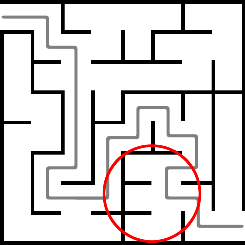
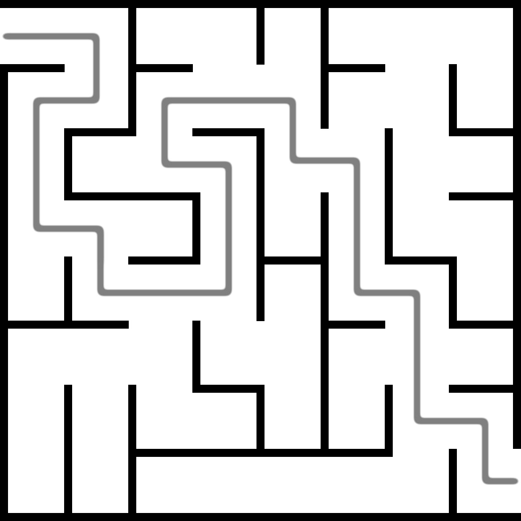
Figure 2: Random Mazes. Mazes generated through a combination of minimum spanning tree edge and weight constraints, and a constraint on the length of the path from start to finish. On the left, an un-optimized maze, with awkward, comb-structured walls (circled). On the right, an optimized maze, generated in seconds by MonoSat.

The solver must then select a set of edges in $G_{1}$ to enable and disable such that the minimum spanning tree of the resulting graph is a) connected and b) results in a maze with a shortest start-to-finish path within the requested bounds. By itself, these constraints can result in poor-quality mazes (see Figure 2, left, and notice the unnatural wall formations near the bottom right corner); by allowing the edges in $G_{1}$ to be enabled or disabled freely, any tree can become the minimum spanning tree, effectively eliminating the effect of the random edge weight constraints.

Instead we convert this into an optimization problem, by combining it with an additional constraint: that the minimum spanning tree of $G_{1}$ must be $\leq$ to some constant, which we then lower repeatedly until it cannot be lowered any further without making the instance unsatisfiable (clasp supports this operation via the “#minimize” statement). This produces plausible mazes (see Figure 2, right), while satisfying our shortest path constraints.

Preemptive Scheduling for Uniprocessors:

Preemptive uniprocessor scheduling, by itself, isn’t a very interesting theory, but we demonstrate how much more expressive it can be when combined with general Boolean reasoning. Our example is a randomized scheduling problem with 1000 tasks and a parameter slack. Each $task_{i}$ has a random duration of 1 to 5 seconds, an arrival time in the range $(0,1000-\textit{slack})$, and a deadline at the task’s arrival time + slack. We model multiprocessor scheduling by creating 10 separate uniprocessor theory solvers $P_{0}\ldots P_{9}$. The processors are heterogenous, with each processor $P$ having a slowdown factor $1\leq s_{P}\leq 2$. Accordingly, for each $task_{i}$, we instantiate theory atoms $task(A_{i},s_{P}\cdot L_{i},D_{i},P_{p})$ for each processor $P_{p}$. We enforce via SAT constraints that each $task_{i}$ be scheduled on exactly one processor. We further

Scheduling	MonoSat	clasp
Slack=10	73s	30s
Slack = 25	70s	Timeout
Slack = 50	38s	Timeout
Slack = 100	47s	Timeout

Table 6: Preemptive Scheduling for Uniprocessors. $J$ is the number of jobs; and $S$ is $\max{slack}$ of any task. Notice: These results are preliminary.

extend our example to model transactions (groups of tasks that must be scheduled in an all-or-none manner), by randomly partitioning the tasks into groups of 10, and enforcing that the jobs in each partitioned are either all scheduled (not necessarily on the same processor), or not scheduled at all. Finally, we enforce that exactly half of these tasks are successfully scheduled.

Table 6 shows that for very small slack times ($slack=10$), clasp is faster than MonoSat, but as the slack grows to even moderate sizes, the ASP encoding quickly becomes impractical to solve, while MonoSat scales efficiently.

7 Conclusion

We have introduced the concept of a monotonic theory and showed a systematic technique to build efficient SMT solvers incorporating such theories. Our technique leverages common-place, highly efficient algorithms for fully specified problem instances, in order to achieve efficient theory propagation and clause learning from the partially specified instances that arise in a lazy SMT approach. We demonstrate the generality of the monotonic theory concept by providing several example theories drawn from graph theory, and one theory to illustrate how typical constrained optimization problems yield monotonic theories. These example theories are expressive — permitting compact encodings for real problems arising from procedural content generation and scheduling — and the SMT solvers we produce via our technique (and standard, unmodified graph and scheduling algorithms) perform well in practice.

As mentioned earlier, fully dynamic algorithms are available for all graph properties considered here (e.g., [12, 20, 21, 13, 22]). These dynamic algorithms permit efficient recomputation of graph properties as edges are added to and removed from a graph, without having to start from scratch each time. So far, we have not explored this direction, but it is a clear avenue for future improvement. The most immediate direction for future work, however, is to discover additional monotonic theories and new application domains that can benefit from them.

References

- [1] Chitta Baral. Knowledge representation, reasoning and declarative problem solving. Cambridge University Press, 2003.
- [2] Georg Boenn, Martin Brain, Marina De Vos, et al. Automatic composition of melodic and harmonic music by answer set programming. In Logic Programming, pages 160–174. Springer, 2008.
- [3] Aaron R Bradley and Zohar Manna. Checking safety by inductive generalization of counterexamples to induction. In Formal Methods in Computer Aided Design, 2007. FMCAD’07, pages 173–180. IEEE, 2007.
- [4] Aaron R Bradley and Zohar Manna. Property-directed incremental invariant generation. Formal Aspects of Computing, 20(4-5):379–405, 2008.
- [5] Leonardo De Moura and Nikolaj Bjorner. Z3: An efficient SMT solver. In Tools and Algorithms for the Construction and Analysis of Systems, pages 337–340. Springer, 2008.
- [6] Leonardo de Moura and Nikolaj Bjørner. Satisfiability modulo theories: An appetizer. In Formal Methods: Foundations and Applications, pages 23–36. Springer, 2009.
- [7] Edsger W Dijkstra. A note on two problems in connexion with graphs. Numerische mathematik, 1(1):269–271, 1959.
- [8] Jack Edmonds and Richard M Karp. Theoretical improvements in algorithmic efficiency for network flow problems. Journal of the ACM (JACM), 19(2):248–264, 1972.
- [9] N. Eén and N. Sörensson. An extensible SAT-solver. In Theory and Applications of Satisfiability Testing, pages 333–336. Springer, 2004.
- [10] Harold N Gabow and Robert Endre Tarjan. A linear-time algorithm for a special case of disjoint set union. Journal of computer and system sciences, 30(2):209–221, 1985.
- [11] Martin Gebser, Benjamin Kaufmann, André Neumann, and Torsten Schaub. clasp: A conflict-driven answer set solver. In Logic Programming and Nonmonotonic Reasoning, pages 260–265. Springer, 2007.
- [12] Monika Rauch Henzinger and Valerie King. Fully dynamic biconnectivity and transitive closure. In Foundations of Computer Science, 1995. Proceedings., 36th Annual Symposium on, pages 664–672. IEEE, 1995.
- [13] Jacob Holm, Kristian de Lichtenberg, and Mikkel Thorup. Poly-logarithmic deterministic fully-dynamic algorithms for connectivity, minimum spanning tree, 2-edge, and biconnectivity. Journal of the ACM (JACM), 48(4):723–760, 2001.
- [14] Joseph B Kruskal. On the shortest spanning subtree of a graph and the traveling salesman problem. Proceedings of the American Mathematical society, 7(1):48–50, 1956.
- [15] Chung Laung Liu and James W Layland. Scheduling algorithms for multiprogramming in a hard-real-time environment. Journal of the ACM (JACM), 20(1):46–61, 1973.
- [16] Joao Marques-Silva, Mikoláš Janota, and Anton Belov. Minimal sets over monotone predicates in boolean formulae. In Computer Aided Verification, pages 592–607. Springer, 2013.
- [17] R. Sebastiani. Lazy satisfiability modulo theories. Journal on Satisfiability, Boolean Modeling and Computation (JSAT), 3:141–224, 2007.
- [18] Adam M Smith and Michael Mateas. Variations forever: Flexibly generating rulesets from a sculptable design space of mini-games. In Computational Intelligence and Games (CIG), 2010 IEEE Symposium on, pages 273–280. IEEE, 2010.
- [19] Adam M Smith and Michael Mateas. Answer set programming for procedural content generation: A design space approach. Computational Intelligence and AI in Games, IEEE Transactions on, 3(3):187–200, 2011.
- [20] Mikkel Thorup. Undirected single-source shortest paths with positive integer weights in linear time. Journal of the ACM (JACM), 46(3):362–394, 1999.
- [21] Mikkel Thorup. Near-optimal fully-dynamic graph connectivity. In Proceedings of the thirty-second annual ACM symposium on Theory of computing, pages 343–350. ACM, 2000.
- [22] Mikkel Thorup. Fully-dynamic min-cut. In Proceedings of the thirty-third annual ACM symposium on Theory of computing, pages 224–230. ACM, 2001.