Determination of electron-hole correlation length in CdSe quantum dots using explicitly correlated two-particle cumulant

Abstract

  ABSTRACT: The electron-hole correlation length serves as an intrinsic length scale for analyzing excitonic interactions in semiconductor nanoparticles. In this work, the derivation of electron-hole correlation length using the two-particle reduced density is presented. The correlation length was obtained by first calculating the electron-hole cumulant from the pair density, and then transforming the cumulant into intracular coordinates, and finally then imposing exact sum-rule conditions on the radial integral of the cumulant. The excitonic wave function for the calculation was obtained variationally using the electron-hole explicitly correlated Hartree-Fock method. As a consequence, both the pair density and the cumulant were explicit functions of the electron-hole separation distance. The use of explicitly correlated wave function and the integral sum-rule condition are the two key features of this derivation. The method was applied to a series of CdSe quantum dots with diameters 1-20 nm and the effect of dot size on the correlation length was analyzed.  

I Introduction

Electron-hole excitations in semiconductor quantum dots are influenced by their size, shape and chemical composition. Controlling the generation and the dissociation of electron-hole (eh) pairs have important technological applications in the field of light-harvesting materialsZhu et al. (2011); Wu et al. (2013); Grätzel (2005); Kamat (2008), photovoltaicsLi et al. (2014); Golobostanfard and Abdizadeh (2014); Mcdonald et al. (2005); Chetia et al. (2014), solid-state lightingAnikeeva et al. (2007); Jang et al. (2010); Sohn et al. (2014); Shea-Rohwer et al. (2013) and lasingKlimov et al. (2000); Foucher et al. (2014); Wu and Asryan (2014); Wang et al. (2014). In order to control the generation and dissociation of the eh-pair, it is important to understand the underlying interaction between the quasiparticles. Theoretical treatment of electron-hole interaction in quantum dots is challenging because of the computational bottleneck associated with quantum mechanical treatment of many-electron systems. In principle, a simplified description of the electron-hole pair can be achieved by ignoring the eh interaction and treating them as independent quasiparticles. Although this approach can dramatically reduce the computational cost, such simplification can lead to qualitatively wrong results. For example, optical spectra calculation using independent quasiparticle approach often shows significant deviation from the experimental results. One of the main limitations of the independent quasiparticle method is its inability in describing bound excitonic states. Multiexcitonic interaction, exciton and biexciton binding energies, radiative and Auger recombination are some of the properties whose calculations depend on the accurate treatment of electron-hole correlation. Theoretical investigation of electron-hole correlation has been performed using various methods such as time-dependent density functional theory (TDDFT)Malloci et al. (2012); Castro et al. (2012); Ullrich and Vignale (2000); Fischer et al. (2012); Hyeon-Deuk and Prezhdo (2012); Badaeva et al. (2011); del Puerto et al. (2006); Troparevsky et al. (2003), perturbation theoryNeuhauser et al. (2013), GW combined with Bethe-Salpeter equationJanis and Pokorny (2012); Pal et al. (2010, 2011); Perebeinos et al. (2005); Puschnig and Ambrosch-Draxl (2002); Rohlfing and Louie (1998); Jiang et al. (2013); Ping et al. (2012); Rohlfing and Louie (2000), configuration interactionBrasken et al. (2002); Corni et al. (2003a, b); Hu et al. (1990); He et al. (2005); Franceschetti and Zunger (2001); An et al. (2007); Rabani et al. (1999); Farmanzadeh and Tabari (2013), quantum Monte CarloHu et al. (1990); Shumway (2006); Shumway and Ceperley (2005); Zhu et al. (1996), path-integral Monte Carlo,Harowitz et al. (2005); Harowitz and Shumway (2005) explicitly correlated Hartree-Fock method,Elward and Chakraborty (2013); Elward et al. (2012a, b, c); Blanton et al. (2013) and electron-hole density functional theory.Sander et al. (1973)

In this work, we are interested in the calculation of electron-hole correlation length (eh-CL) in CdSe quantum dots. Our goal is to provide a statistical definition of the electron-hole correlation length. The concept of correlation length has been widely used in many fields, including statistical mechanicsBrush (1967); Middleton and Fisher (2002); Middleton and Wingreen (1993); Thomas and Middleton (2009) and polymer science.Domb and Joyce (1972); Gujrati (1998); Spouge (1988); Vilenkin (1978); Middleton and Fisher (2002); Middleton and Wingreen (1993); Thomas and Middleton (2009) One of the important features of the eh-CL is that is it provides an intrinsic length scale for describing the electron-hole interaction. Because of this, it can play an important role in describing excitonic effects in quantum dots and other nanomaterials such as carbon nanotubes.Luer et al. (2009); Koch et al. (2003); Corfdir et al. (2013) The eh-CL can also be used for construction of electron-hole correlation functional for multicomponent density functional theory.Sander et al. (1973) For example, Salahub and co-workers have developed a series of exchange-correlation functions that are based on electron-electron correlation lengthProynov and Salahub (1994); Proynov et al. (1994a, b, 1995) and a similar strategy can be used for construction of electron-hole correlation functionals using eh-CL. The eh-CL can also aid in the development of explicitly correlated wave functions (such as Jastrow and Gaussian-type geminal functions) which depend directly on the electron-hole separation distance.Zhu et al. (1996); Elward and Chakraborty (2013); Elward et al. (2012a, b, c); Blanton et al. (2013)

We have used the 2-particle electron-hole density matrix for the definition and calculation of the eh-CL. Two-particle reduced density matrix (2-RDM) has been used extensively for investigation of electron-electron correlationMazziotti (2006, 2007, 2012a); Rohr et al. (2010); Rohr and Pernal (2011); Rajam et al. (2010); Elliott and Maitra (2011) and electronic excitationChatterjee and Pernal (2012) in many-electron systems. For the present system, the 2-RDM is the appropriate mathematical quantity that contains all the necessary information about electron-hole correlation. Specifically, the cumulant associated with the electron-hole 2-RDM is the component of the 2-RDM that cannot be expressed as a product of 1-particle electron and hole densities. In principle, the 2-RDM can be obtained directly without the need for an underlying wave function as long as the $N$-representability of 2-RDM can be satisfied. However, in the present work, we have obtained the 2-RDM from an explicitly correlated electron-hole wave function. The remainder of the article is organized as follows. The derivation of eh-CL from the electron-hole cumulant is presented in subsection II.1, transformation to intracular and extracular coordinates is described in subsection II.2, and details of the explicitly correlated electron-hole wave function are presented in subsection II.3 and section III. The method was applied to a series of CdSe quantum dots and the results are presented in section IV.

II Theory

II.1 Electron-hole cumulant

The interaction between the quasiparticles in the quantum dot is described the electron-hole HamiltonianZhu et al. (1996); Hu et al. (1990); Burovski et al. (2001); Wimmer et al. (2006); Woggon (2013); Braskan et al. (2001); Corni et al. (2003a, b, c); Vanska et al. (2006); Vänskä and Sundholm (2010); Sundholm and Vanska (2012); Blanton et al. (2013); Elward and Chakraborty (2013); Elward et al. (2012a, c) which has the following general expression

$$H =\sum_{ij}\langle i|\frac{-\hbar^{2}}{2m_{\mathrm{e}}}\nabla^{2}_{\mathrm{e}}+v_{\mathrm{ext}}^{\mathrm{e}}|j\rangle e_{i}^{\dagger}e_{j}$$ (1)

$$+\sum_{ij}\langle i|\frac{-\hbar^{2}}{2m_{\mathrm{h}}}\nabla^{2}_{\mathrm{h}}+v_{\mathrm{ext}}^{\mathrm{h}}|j\rangle h^{\dagger}_{i}h_{j}$$

$$+\sum_{iji^{\prime}j^{\prime}}\langle iji^{\prime}j^{\prime}|\epsilon^{-1}r_{\mathrm{eh}}^{-1}|iji^{\prime}j^{\prime}\rangle e^{\dagger}_{i}e_{j}h_{i^{\prime}}^{\dagger}h_{j^{\prime}}$$

$$+\sum_{ijkl}w_{ijkl}^{\mathrm{ee}}e^{\dagger}_{i}e_{j}^{\dagger}e_{l}e_{k}+\sum_{ijkl}w_{ijkl}^{\mathrm{hh}}h^{\dagger}_{i}h_{j}^{\dagger}h_{l}h_{k}.$$

We define the electron-hole wave function for a multiexcitonic system consisting of $N_{\mathrm{e}}$ and $N_{\mathrm{h}}$ number of electrons and holes, respectively by $\Psi_{\mathrm{eh}}(\mathbf{x}_{1}^{\mathrm{e}},\dots,\mathbf{x}_{N_{\mathrm{e}}}^{\mathrm{e}},\mathbf{x}_{1}^{\mathrm{h}},\dots,\mathbf{x}_{N_{\mathrm{h}}}^{\mathrm{h}})$, where $\mathbf{x}$ is a compact notation for both the spatial and spin coordinate of the particles. The spin-integrated 2-particle reduced density can be obtained from the electron-hole wave function by integration over the $N_{\mathrm{e}}-1$ and $N_{\mathrm{h}}-1$ coordinates as shown in the following equation

$$\rho_{\mathrm{eh}}(\mathbf{r}^{\mathrm{e}},\mathbf{r}^{\mathrm{h}}) =\frac{N_{\mathrm{e}}N_{\mathrm{h}}}{\langle\Psi_{\mathrm{eh}}|\Psi_{\mathrm{eh}}\rangle}\int ds_{1}^{\mathrm{e}}ds_{1}^{\mathrm{h}}d\mathbf{x}_{2}^{\mathrm{e}},\dots,\mathbf{x}_{N_{\mathrm{e}}}^{\mathrm{e}}\mathbf{x}_{2}^{\mathrm{h}},\dots,\mathbf{x}_{N_{\mathrm{h}}}^{\mathrm{h}}\Psi_{\mathrm{eh}}^{\ast}\Psi_{\mathrm{eh}}$$ (2)

where, integration over the spin coordinate $s_{1}$ is performed for both electron and hole. The single-particle density is obtained from the 2-particle density using the sum-rule conditionParr and Yang (1989)

$$\rho_{\mathrm{e}}(\mathbf{r}^{\mathrm{e}}) =\frac{1}{N_{\mathrm{h}}}\int d\mathbf{r}^{\mathrm{h}}\rho_{\mathrm{eh}}(\mathbf{r}^{\mathrm{e}},\mathbf{r}^{\mathrm{h}}),$$ (3)

$$\rho_{\mathrm{h}}(\mathbf{r}^{\mathrm{h}}) =\frac{1}{N_{\mathrm{e}}}\int d\mathbf{r}^{\mathrm{e}}\rho_{\mathrm{eh}}(\mathbf{r}^{\mathrm{e}},\mathbf{r}^{\mathrm{h}}).$$ (4)

We define the electron-hole cumulant as the difference between the 2-particle density and the product of the 1-particle electron and hole densities as shown in the following equation

$$q(\mathbf{r}^{\mathrm{e}},\mathbf{r}^{\mathrm{h}}) =\rho_{\mathrm{eh}}(\mathbf{r}^{\mathrm{e}},\mathbf{r}^{\mathrm{h}})-\rho_{\mathrm{e}}(\mathbf{r}^{\mathrm{e}})\rho_{\mathrm{h}}(\mathbf{r}^{\mathrm{h}}).$$ (5)

This definition is analogous to the definition used by Mazziotti et al.Juhasz and Mazziotti (2006) in electronic structure theory. By construction, the cumulant contains information about correlation between the two particles. Consequently, the Coulomb contribution of the electron-hole correlation energy can be directly expressed in terms of the electron-hole cumulant and is given by the following expression

$$\langle\Psi_{\mathrm{eh}}|V_{\mathrm{eh}}|\Psi_{\mathrm{eh}}\rangle =\langle\rho_{\mathrm{eh}}\epsilon^{-1}r_{\mathrm{eh}}^{-1}\rangle$$ (6)

$$=J_{\mathrm{eh}}+\langle q(\mathbf{r}^{\mathrm{e}},\mathbf{r}^{\mathrm{h}})\epsilon^{-1}r_{\mathrm{eh}}^{-1}\rangle,$$

where $\epsilon$ is the dielectric constant and $J_{\mathrm{eh}}$ is the classical Coulomb electron-hole energy

$$J_{\mathrm{eh}} =\langle\rho_{\mathrm{e}}\rho_{\mathrm{h}}\epsilon^{-1}r_{\mathrm{eh}}^{-1}\rangle.$$ (7)

The cumulant has an important property that its integration over all space should be zero due to the density sum-rule conditionsParr and Yang (1989)

$$\int d\mathbf{r}^{\mathrm{e}}d\mathbf{r}^{\mathrm{h}}q(\mathbf{r}^{\mathrm{e}},\mathbf{r}^{\mathrm{h}}) =0.$$ (8)

We use this relationship for the definition of the electron-hole correlation length.

II.2 Intracular and extracular coordinates

Beginning with Coleman’s initial definition of the intracule and extacule matrices in terms of the center of mass (extracule) and relative motion (intracule) coordinates,Coleman (1967) the concept of the intracule and extracule in the regime of electronic systems has been previously explored in earlier studies.Coleman (1967); Ugalde et al. (1991); Koga and Matsuyama (1998); Gill et al. (2000, 2003); Besley et al. (2003); Gill et al. (2006) The intracular and extracular coordinates for the eh-system are defined by

$$\mathbf{r}_{\mathrm{eh}} =\mathbf{r}^{\mathrm{e}}-\mathbf{r}^{\mathrm{h}}$$ (9)

$$\mathbf{R} =\frac{1}{2}\left(\mathbf{r}^{\mathrm{e}}+\mathbf{r}^{\mathrm{h}}\right).$$ (10)

The integral of the cumulant is expressed in terms of these coordinates

$$\int d\mathbf{r}^{\mathrm{e}}d\mathbf{r}^{\mathrm{h}}q(\mathbf{r}^{\mathrm{e}},\mathbf{r}^{\mathrm{h}}) =\int d\mathbf{r}_{\mathrm{eh}}\int d\mathbf{R}q(\mathbf{r}_{\mathrm{eh}},\mathbf{R})$$ (11)

$$=\int_{0}^{\infty}d{r}_{\mathrm{eh}}r^{2}_{\mathrm{eh}}\int d\Omega\sin\theta\int d\mathbf{R}q(\mathbf{r}_{\mathrm{eh}},\mathbf{R})$$ (12)

$$=\int_{0}^{\infty}d{r}_{\mathrm{eh}}r^{2}_{\mathrm{eh}}q_{\mathrm{r}}(r_{\mathrm{eh}})$$ (13)

In the above expression, the integral over the intracular coordinate $\mathbf{r}_{\mathrm{eh}}$ is transformed into spherical polar coordinates. The function $q_{r}$ is the spherically averaged radial cumulant and the integral of the radial cumulant over a finite limit is used to define the following function $I(d)$

$$I(d)=\int_{0}^{d}dr_{\mathrm{eh}}r^{2}_{\mathrm{eh}}q_{r}(r_{\mathrm{eh}}).$$ (14)

The zero-integral property of $q$ (defined in Eq. (8)) ensures that this integral goes to zero at large $d$

$$\lim_{d\rightarrow\infty}I(d)=0.$$ (15)

Here, we use $I(d)$ to define the electron-hole correlation length. Specifically, the electron-hole correlation length ($r_{\mathrm{c}}$) is defined as the value of $d$ at which the value of $I(d)$ is zero

$$|I(r_{\mathrm{c}})| =0\quad\quad r_{\mathrm{c}}<<\infty.$$ (16)

The description of the electron-hole wave function used for the calculation of the radial cumulant is presented in the following section.

II.3 Explicitly correlated electron-hole wave function

We have used the electron-hole explicitly correlated Hartree-Fock method (eh-XCHF) for obtaining the electron-hole wave function. This method has been used in earlier work for the computation of exciton binding energies and electron-hole recombination probabilities in quantum dots.Elward et al. (2012a, b, c); Elward and Chakraborty (2013); Blanton et al. (2013) A brief summary of the eh-XCHF method is presented here and the implementation details of this method can be found in work by Elward and co-workers.Elward et al. (2012a, b, c) The ansatz of the eh-XCHF wave function consists of multiplying the mean-field electron-hole reference wave functions with an explicitly correlated function $G$ as shown in the following equation

$$\Psi_{\mathrm{eh-XCHF}}=G\Phi_{\mathrm{e}}\Phi_{\mathrm{h}},$$ (17)

where $G$ is the geminal operator

$$G =\sum_{i=1}^{N_{\mathrm{{e}}}}\sum_{j=1}^{N_{\mathrm{{h}}}}g(r_{ij}),$$ (18)

$$g(r_{\mathrm{eh}}) =\sum_{k=1}^{N_{\mathrm{{g}}}}b_{k}\exp(-\gamma_{k}r_{\mathrm{eh}}^{2}).$$ (19)

The eh-XCHF method is a variational method in which the correlation function $G$ and the reference wave function are obtained by minimizing the total energy

$$E_{\mathrm{eh-XCHF}} =\min_{G,\Phi_{\mathrm{e}},\Phi_{\mathrm{h}}}\frac{\langle G\Phi_{0}|H|G\Phi_{0}\rangle}{\langle G\Phi_{0}|G\Phi_{0}\rangle},$$ (20)

where $\Phi_{0}=\Phi_{\mathrm{e}}\Phi_{\mathrm{h}}$. To perform the above minimization, it is more efficient to work with the following congruent-transformed operators

$$\tilde{H} =G^{\dagger}HG,$$ (21)

$$\tilde{1} =G^{\dagger}G.$$ (22)

This transformation is particularly important for the calculation of the 2-particle reduced density matrix in the present work. The set of parameters $\{b_{k},\gamma_{k}\}$ in $G$ were obtained by non-linear optimization, and for a given set of these parameters, the minimization over the reference wave function was performed by determining the self-consistent solution of the coupled Fock equations

$$\tilde{\mathbf{F}}_{\mathrm{e}}\mathbf{C}_{\mathrm{e}} =\tilde{\mathbf{S}}_{\mathrm{e}}\mathbf{C}_{\mathrm{e}}\lambda_{\mathrm{e}},$$ (23)

$$\tilde{\mathbf{F}}_{\mathrm{h}}\mathbf{C}_{\mathrm{h}} =\tilde{\mathbf{S}}_{\mathrm{h}}\mathbf{C}_{\mathrm{h}}\lambda_{\mathrm{h}}.$$ (24)

The tilde in the above expressions represent that the Fock and the overlap matrices incorporate the transformed operators defined in Eq. (21).

The transformed operator $\tilde{1}$ can be written as a sum of operators as shown below

$$\tilde{1} =G^{\dagger}G$$ (25)

$$=\sum_{ii^{\prime}}g(i,i^{\prime})\sum_{jj^{\prime}}g(j,j^{\prime})\quad(i,j=1,\dots,N_{\mathrm{e}};i^{\prime},j^{\prime}=1,\dots,N_{\mathrm{h}})$$ (26)

$$=\sum_{ii^{\prime}}g(i,i^{\prime})g(i,i^{\prime})+\sum_{i\neq j,i^{\prime}}g(i,i^{\prime})g(j,i^{\prime})$$ (27)

$$+\sum_{i^{\prime}\neq j^{\prime},i}g(i,i^{\prime})g(i,j^{\prime})+\sum_{i\neq j,i^{\prime}\neq j^{\prime}}g(i,i^{\prime})g(j,j^{\prime}).$$

The above expression can be written in a compact notation as a sum of 2, 3, and 4-particle operators

$$G^{\dagger}G =\Omega_{11}+\Omega_{21}+\Omega_{12}+\Omega_{22}.$$ (28)

The 2-particle density for the eh-XCHF wave function can be expressed in terms of these operators as shown below

$$\rho_{\mathrm{eh}}(\mathbf{r}^{\mathrm{e}},\mathbf{r}^{\mathrm{h}}) =\frac{N_{\mathrm{e}}N_{\mathrm{h}}}{\langle\Psi_{\mathrm{eh-XCHF}}|\Psi_{\mathrm{eh-XCHF}}\rangle}$$ (29)

$$\times\langle\Psi_{\mathrm{eh-XCHF}}^{\ast}\Psi_{\mathrm{eh-XCHF}}\rangle_{s_{1},s_{1}^{\prime},2,2^{\prime},\dots,N_{\mathrm{e}},N_{\mathrm{h}}},$$

where the subscript in the above expression is a compact notation for integration over the remaining coordinates described in Eq. (2). Substituting the expression from Eq. (28), we get the following expression

$$\rho_{\mathrm{eh}}(\mathbf{r}^{\mathrm{e}},\mathbf{r}^{\mathrm{h}}) =\frac{N_{\mathrm{e}}N_{\mathrm{h}}}{\langle\Phi_{0}|\tilde{1}|\Phi_{0}\rangle}$$ (30)

$$\times\langle\Phi_{0}^{\ast}(\Omega_{11}+\Omega_{12}+\Omega_{21}+\Omega_{22})\Phi_{0}\rangle_{s_{1},s_{1}^{\prime},2,2^{\prime},\dots,N_{\mathrm{e}},N_{\mathrm{h}}}.$$

For a multiexcitonic system all 2, 3, and 4-particle operators should be used for the computation of the 2-particle density. In a related work on many-electron system, we have shown that it is possible to avoid integration over higher-order operators by using diagrammatic summation technique and a similar strategy can be used for multiexcitonic systems as well.Bayne et al. (2014)

II.4 Relation to uncorrelated transition density matrices

One of the important features of the correlation function is that it allows for a compact representation of the 2-particle density matrix in the position representation. The relationship can be readily seen by expanding the eh-XCHF wave function in the Slater determinant basis

$$G\Phi_{0}=\sum_{ii^{\prime}}^{\infty}\underbrace{\textbullet\langle\Phi_{i}^{\mathrm{e}}\Phi_{i^{\prime}}^{\mathrm{h}}|G|\Phi_{0}^{\mathrm{e}}\Phi_{0}^{\mathrm{h}}\rangle}_{c_{ii^{\prime}}}\Phi_{i}^{\mathrm{e}}\Phi_{i^{\prime}}^{\mathrm{h}}=\sum_{ii^{\prime}}^{\infty}c_{ii^{\prime}}\Phi_{i}^{\mathrm{e}}\Phi_{i^{\prime}}^{\mathrm{h}}.$$ (31)

Substituting Eq. (31) in the expression of $\rho_{\mathrm{eh}}$ gives

$$\rho_{\mathrm{eh}}(\mathbf{r}^{\mathrm{e}},\mathbf{r}^{\mathrm{h}}) =\frac{N_{\mathrm{e}}N_{\mathrm{h}}}{\langle\Phi_{0}|\tilde{1}|\Phi_{0}\rangle}$$ (32)

$$\times\langle\sum_{ij}^{\infty}\sum_{i^{\prime}j^{\prime}}^{\infty}c_{ii^{\prime}}^{\ast}c_{jj^{\prime}}\Phi_{i}^{\mathrm{e}\ast}\Phi_{i^{\prime}}^{\mathrm{h}\ast}\Phi_{j}^{\mathrm{e}}\Phi_{j^{\prime}}^{\mathrm{h}}\rangle_{s_{1},s_{1}^{\prime},2,2^{\prime},\dots,N_{\mathrm{e}},N_{\mathrm{h}}}$$

$$=\frac{N_{\mathrm{e}}N_{\mathrm{h}}}{\langle\Phi_{0}|\tilde{1}|\Phi_{0}\rangle}\sum_{ij}^{\infty}\sum_{i^{\prime}j^{\prime}}^{\infty}c_{ii^{\prime}}^{\ast}c_{jj^{\prime}}d_{ij}^{\mathrm{e}}d_{i^{\prime}j^{\prime}}^{\mathrm{h}},$$ (33)

where the transition density matrix $d_{ij}$ is defined as

$$d_{ij}^{\mathrm{e}}(\mathbf{r}^{\mathrm{e}}) =\langle\Phi_{i}^{\mathrm{e}\ast}\Phi_{j}^{\mathrm{e}}\rangle_{s_{1},2,\dots,N_{\mathrm{e}}}.$$ (34)

It is seen from Eq. (32) that the 2-particle density obtained from the eh-XCHF wave function is equivalent to the infinite-order expansion in terms of the transition density matrices.

III Computational details

The method described in section II was used for calculating electron-hole correlation length in CdSe quantum dots in the range of 1-20 nm in diameter. We are interested in the effect of dot size on the electron-hole correlation length for a single electron-hole pair in CdSe quantum dots. For a single electron-hole pair, the higher-order operators in Eq. (30) rigorously vanish from the expression. This provides considerable simplification in the calculation of the 2-particle density. Because of the dot size, application of either DFT or atom-centered pseudopotential approach is computationally prohibitive. To make the computation tractable, we have used a parabolic confining potential in the electron-hole Hamiltonian described in Eq. (1). Parabolic confinement potential in quantum dots has been used extensively for various properties such as total exciton energyEl-Said (1994); Que (1992), exciton dissociationNenashev et al. (2011), exciton binding energyPoszwa (2010); Elward et al. (2012a, c); Elward and Chakraborty (2013) eh-recombination probabilityElward et al. (2012a, b); Elward and Chakraborty (2013), effect of magneticJaziri (1994); Halonen et al. (1992); Song and Ulloa (2001); Taut et al. (2009); Kolovsky et al. (2014); Trojnar et al. (2011) and electric fieldsJaziri (1994); Xie (2009); He and Xie (2010); Blanton et al. (2013); Fernandez and Summers (2013), exciton-polariton condensateFernandez et al. (2013), linear optical propertiesRey et al. (2005); Kim et al. (2007), optical rectificationRezaei et al. (2011), non-linear rectificationXie (2009), dynamicsLiu et al. (2011), eh-correlation energyBlundell and Joshi (2010); Zhao et al. (2011), resonant tunnelingTeichmann et al. (2013), collective modesMorales et al. (2008), and thermodynamic propertiesNammas et al. (2011). The external potential for the electron and hole quasiparticle was defined as

$$v_{\alpha}^{\mathrm{ext}}=\frac{1}{2}k_{\alpha}|\mathbf{r}_{\alpha}|^{2}\quad\alpha=\mathrm{e,h}$$ (35)

where $k_{\alpha}$ is the force constant which determines the strength of the confinement potential. We have used a particle-number based search procedure for determination of the force constant $k_{\alpha}$. The central idea of this approach is to find the value of $k_{\alpha}$ such that the computed 1-particle electron and hole densities are confined within the volume of the quantum dot. This is obtained by performing the following minimization

$$\min_{k_{\alpha}^{\mathrm{min}}}\left(N_{\alpha}-\int_{0}^{\frac{D_{\mathrm{dot}}}{2}}drr^{2}\int d\Omega\rho_{\alpha}(\mathbf{r})\right)^{2},$$ (36)

where $D_{\mathrm{dot}}$ is the diameter of the quantum dot and $\Omega$ is the angular coordinate. The values of the force constants used for each dot is listed in Table 1.

Table 1: Force constants for CdSe quantum dots.

Dot diameter (nm)	$k_{\mathrm{e}}$ (atomic units)	$k_{\mathrm{h}}$ (atomic units)
$1.24$	$2.66\times 10^{-2}$	$9.10\times 10^{-3}$
$1.79$	$6.22\times 10^{-3}$	$2.13\times 10^{-3}$
$2.76$	$1.10\times 10^{-3}$	$3.76\times 10^{-4}$
$2.98$	$8.10\times 10^{-4}$	$2.77\times 10^{-4}$
$3.28$	$5.52\times 10^{-4}$	$1.89\times 10^{-4}$
$3.79$	$3.09\times 10^{-4}$	$1.06\times 10^{-4}$
$4.80$	$1.20\times 10^{-4}$	$4.12\times 10^{-5}$
$5.00$	$1.02\times 10^{-4}$	$3.51\times 10^{-5}$
$6.60$	$3.40\times 10^{-5}$	$1.16\times 10^{-5}$
$10.00$	$6.41\times 10^{-6}$	$2.19\times 10^{-6}$
$15.00$	$1.26\times 10^{-6}$	$4.33\times 10^{-7}$
$20.00$	$4.01\times 10^{-7}$	$1.37\times 10^{-7}$

The kinetic energy operator was computed using the electron and hole effective masses of $0.13$ and $0.38$ atomic units, respectively.Wimmer et al. (2006) The interaction between the electron and hole was described by screened Coulomb potential. We have used the size and distance dependent dielectric function $\epsilon(\mathbf{r},R_{\mathrm{dot}})$, which was developed by Wang and Zunger for CdSe.Wang and Zunger (1996) The electron and hole molecular orbitals in $\Phi_{0}$ were represented using a linear combination of Gaussian type orbitals (GTOs) and the expansion coefficients were obtained by the solving the coupled Fock equations shown in Eq. (23). The basis used was a single S Cartesian GTO was used and the exponents of the basis functions are listed in Table 2.

Table 2: Exponent used in GTO basis $e^{-\alpha r^{2}}$.

Dot diameter (nm)	$\alpha$ (atomic units)
$1.24$	$2.94\times 10^{-2}$
$1.78$	$1.42\times 10^{-2}$
$2.76$	$5.98\times 10^{-2}$
$2.98$	$5.13\times 10^{-2}$
$3.28$	$4.24\times 10^{-3}$
$3.79$	$3.17\times 10^{-3}$
$4.80$	$1.98\times 10^{-3}$
$5.00$	$1.83\times 10^{-3}$
$6.60$	$1.05\times 10^{-3}$
$10.00$	$4.57\times 10^{-4}$
$15.00$	$2.03\times 10^{-4}$
$20.00$	$1.14\times 10^{-4}$

The use of GTOs is especially convenient because the integrals involving the GTOs and the Gaussian correlation function, $G$, are known analytically.Boys (1950); Singer (1960); Persson and Taylor (1996, 1997) For a given value of $\mathbf{r}^{\mathrm{e}}$, the 1-particle density $\rho$ was calculated analytically. The integration over the intracular coordinate in Eq. (14) was performed numerically. The correlation function, $G$, was expanded as a linear combination of six Guassian-type geminal functionsElward et al. (2012a, c); Elward and Chakraborty (2013) and the set of $\{b_{k},\gamma_{k}\}$ parameters were optimized for each dot size. The first set of geminal parameters was set to $b_{1}=1$ and $\gamma_{1}=0$ for all CdSe dot diameters. For each dot diameter, five sets of geminal parameters were determined sequentially by minimizing the energy. The values of the geminal parameters are found in Table 3.

Table 3: Value of the geminal parameters for CdSe quantum dots.

Dot Diameter (nm)	$b_{2}$	$\gamma_{2}$	$b_{3}$	$\gamma_{3}$	$b_{4}$	$\gamma_{4}$	$b_{5}$	$\gamma_{5}$	$b_{6}$	$\gamma_{6}$
$1.25$	$1.338\times 10^{-1}$	$2.134\times 10^{-2}$	$1.559\times 10^{-1}$	$1.150\times 10^{-3}$	$3.630\times 10^{-2}$	$1.112\times 10^{0}$	$2.290\times 10^{-2}$	$2.111\times 10^{-1}$	$1.099\times 10^{-1}$	$1.020\times 10^{-3}$
$1.78$	$1.497\times 10^{-1}$	$1.569\times 10^{-2}$	$2.099\times 10^{-1}$	$1.120\times 10^{-3}$	$2.009\times 10^{-1}$	$4.400\times 10^{-4}$	$4.260\times 10^{-2}$	$1.112\times 10^{0}$	$3.820\times 10^{-2}$	$1.444\times 10^{-1}$
$2.76$	$2.279\times 10^{-1}$	$4.700\times 10^{-3}$	$5.990\times 10^{-2}$	$1.111\times 10^{-1}$	$2.119\times 10^{-1}$	$4.400\times 10^{-4}$	$-1.910\times 10^{-2}$	$3.140\times 10^{-3}$	$1.540\times 10^{-2}$	$1.222\times 10^{0}$
$2.98$	$2.449\times 10^{-1}$	$3.960\times 10^{-3}$	$6.400\times 10^{-2}$	$1.114\times 10^{-1}$	$2.099\times 10^{-1}$	$3.700\times 10^{-4}$	$1.490\times 10^{-2}$	$1.434\times 10^{0}$	$1.580\times 10^{-2}$	$1.012\times 10^{-1}$
$3.28$	$2.589\times 10^{-1}$	$3.580\times 10^{-3}$	$6.680\times 10^{-2}$	$1.112\times 10^{-1}$	$2.109\times 10^{-1}$	$4.300\times 10^{-4}$	$9.990\times 10^{-2}$	$1.100\times 10^{-4}$	$1.590\times 10^{-2}$	$1.253\times 10^{0}$
$3.79$	$2.799\times 10^{-1}$	$3.000\times 10^{-3}$	$6.990\times 10^{-2}$	$1.111\times 10^{-1}$	$2.209\times 10^{-1}$	$3.700\times 10^{-4}$	$1.099\times 10^{-1}$	$1.200\times 10^{-4}$	$1.540\times 10^{-2}$	$1.432\times 10^{0}$
$4.80$	$3.610\times 10^{-1}$	$1.660\times 10^{-3}$	$8.790\times 10^{-2}$	$1.010\times 10^{-1}$	$6.180\times 10^{-2}$	$2.229\times 10^{-2}$	$2.099\times 10^{-1}$	$2.200\times 10^{-4}$	$9.990\times 10^{-2}$	$1.100\times 10^{-4}$
$5.00$	$3.699\times 10^{-1}$	$1.570\times 10^{-3}$	$8.990\times 10^{-2}$	$1.010\times 10^{-1}$	$6.680\times 10^{-2}$	$2.135\times 10^{-2}$	$2.099\times 10^{-1}$	$2.200\times 10^{-4}$	$9.990\times 10^{-2}$	$1.100\times 10^{-4}$
$6.60$	$4.499\times 10^{-1}$	$1.380\times 10^{-3}$	$6.099\times 10^{-1}$	$1.800\times 10^{-4}$	$5.280\times 10^{-2}$	$1.112\times 10^{0}$	$1.299\times 10^{-1}$	$1.011\times 10^{-1}$	$1.331\times 10^{-1}$	$1.335\times 10^{-2}$
$10.00$	$5.899\times 10^{-1}$	$1.240\times 10^{-3}$	$9.999\times 10^{-1}$	$1.300\times 10^{-4}$	$6.400\times 10^{-2}$	$1.012\times 10^{0}$	$1.569\times 10^{-1}$	$1.023\times 10^{-1}$	$1.799\times 10^{-1}$	$1.211\times 10^{-2}$
$15.00$	$6.999\times 10^{-1}$	$1.040\times 10^{-3}$	$1.110\times 10^{0}$	$1.300\times 10^{-4}$	$6.580\times 10^{-2}$	$1.102\times 10^{0}$	$1.589\times 10^{-1}$	$1.022\times 10^{-1}$	$1.999\times 10^{-1}$	$1.999\times 10^{-1}$
$20.00$	$7.999\times 10^{-1}$	$1.030\times 10^{-3}$	$2.000\times 10^{0}$	$1.200\times 10^{-4}$	$9.999\times 10^{-1}$	$4.000\times 10^{-5}$	$5.489\times 10^{-1}$	$1.227\times 10^{-2}$	$2.899\times 10^{-1}$	$1.240\times 10^{-3}$

IV Results

The electron-hole correlation length was obtained by integration of the radial cumulant as described in Eq. (14). In Figure 1, the integral of the cumulant, $I(d)$, for three different dot sizes are presented.

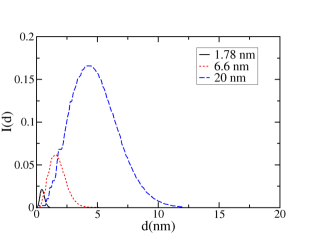
Figure 1: The value of $I(d)$ as $d$, the upper limit in Eq. (14), is varied for the 1.78 nm, 6.6 nm, and 20 nm diameter CdSe quantum dots.

As expected, the integral goes to zero at large distances (high $d$ values) and the distance at which the integral converges to zero is defined as the electron-hole correlation length $r_{\mathrm{c}}$. The calculated electron-hole correlation lengths are presented in Table 4.

Table 4: Electron-hole correlation lengths and $r_{\mathrm{node}}$ for CdSe quantum dots.

Dot Diameter	Correlation length	$r_{\mathrm{node}}$
(nm)	(nm)	(nm)
$1.24$	$0.381$	$0.283$
$1.78$	$0.683$	$0.431$
$2.76$	$1.905$	$0.595$
$2.98$	$2.117$	$0.653$
$3.28$	$2.572$	$0.732$
$3.79$	$2.778$	$0.833$
$4.80$	$3.293$	$1.082$
$5.00$	$3.307$	$1.124$
$6.60$	$4.047$	$1.653$
$10.00$	$6.156$	$2.749$
$15.00$	$10.164$	$3.257$
$20.00$	$11.930$	$4.733$

We find that, in all cases, the correlation length increases with increasing dot diameter. Another quantity that is important for investigating electron-hole correlation is the length scale associated with the first node of the radial cumulant. We define this quantity as $r_{\mathrm{node}}$ and the calculated values are presented in Table 4. The maximum of the $I(d)$ in Figure 1 corresponds to $r_{\mathrm{node}}$. Because the interaction between the electron and hole is attractive, we expect an enhancement in the pair density as compared to mean-field density at small $r_{\mathrm{eh}}$ distances. This phenomenon is opposite to the correlation hole observed in electron-electron interaction, in which small $r_{\mathrm{ee}}$ shows a decrease in correlated electron-pair density as compared to uncorrelated electron density. The $r_{\mathrm{node}}$ can be interpreted as the effective radius of the sphere that encloses the region of enhanced probability density. As seen from Table 4, $r_{\mathrm{c}}$ and $r_{\mathrm{node}}$ are similar in magnitude for small dot sizes, but these quantities differ significantly for larger dots. The correlation length as a function of the dot diameter is plotted in Figure 2. The set of data showed good agreement with the linear fit, with a mean absolute error of 0.323 nm. A trend of increasing correlation length with increasing dot diameter is observed. The correlation lengths show that correlation effects are important even at long electron-hole separations.

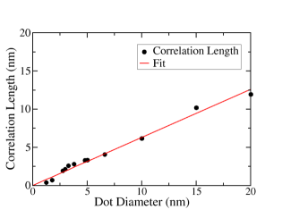
Figure 2: The correlation length as a function of the dot diameter $D_{\mathrm{dot}}$. The linear fit is $r_{\mathrm{C}}=0.6303D_{\mathrm{dot}}$, with a mean absolute error of 0.323 nm.

The linear relationship between the dot diameter and the correlation length has an important application in the construction of compact explicitly correlated electron-hole wave function. For example, the determination of the eh-XCHF wave function requires the optimization of the non-linear parameters $\{b_{k},\gamma_{k}\}$ in $G$. By using the relationship between the dot diameter and correlation length, it is possible to assign the non-linear parameters as some multiple of the correlation length. This approach avoids optimization of non-linear parameters and can result in significant reduction in the computational effort.

V Conclusions

In conclusion, we have presented a method for calculating electron-hole correlation length in semiconductor quantum dots. We have used the cumulant derived from the electron-hole 2-particle density as the central quantity for defining the correlation length. There are two key features of this method. First, the 2-particle reduced density was obtained from an explicitly correlated electron-hole wave function. Consequently, the reduced density matrix and the corresponding cumulant were explicit functions of the electron-hole separation distance. Second, the calculation of the correlation length was not based on the nodes of the cumulant but was derived from the exact sum rule relationship satisfied by all $N$-representable cumulants. The developed method was applied to a series of CdSe quantum dots and a linear relationship between the dot size and correlation length was observed. The electron-hole correlation length provides a natural length scale for investigating electron-hole correlation in nanoparticles. We envision that in future work, the electron-hole correlation length will be used in the construction of compact explicitly correlated wave functions and also for developing multi-componentSander et al. (1973) electron-hole density functionals.

References

- Zhu et al. (2011) Haiming Zhu, Nianhui Song, and Tianquan Lian, “Wave function engineering for ultrafast charge separation and slow charge recombination in type ii core/shell quantum dots,” Journal of the American Chemical Society 133, 8762–8771 (2011).
- Wu et al. (2013) Kaifeng Wu, Zheng Liu, Haiming Zhu, and Tianquan Lian, “Exciton annihilation and dissociation dynamics in group ii–v cd3p2 quantum dots,” The Journal of Physical Chemistry A 117, 6362–6372 (2013).
- Grätzel (2005) Michael Grätzel, “Solar energy conversion by dye-sensitized photovoltaic cells,” Inorganic Chemistry 44, 6841–6851 (2005), pMID: 16180840.
- Kamat (2008) Prashant V. Kamat, “Quantum dot solar cells. semiconductor nanocrystals as light harvesters†,” The Journal of Physical Chemistry C 112, 18737–18753 (2008).
- Li et al. (2014) Zhen Li, Libo Yu, Yingbo Liu, and Shuqing Sun, “Cds/cdse quantum dots co-sensitized tio2 nanowire/nanotube solar cells with enhanced efficiency,” Electrochimica Acta 129, 379 – 388 (2014).
- Golobostanfard and Abdizadeh (2014) Mohammad Reza Golobostanfard and Hossein Abdizadeh, “Tandem structured quantum dot/rod sensitized solar cell based on solvothermal synthesized cdse quantum dots and rods,” Journal of Power Sources 256, 102 – 109 (2014).
- Mcdonald et al. (2005) S.A. Mcdonald, G. Konstantatos, S. Zhang, P.W. Cyr, E.J.D. Klem, L. Levina, and E.H. Sargent, “Solution-processed pbs quantum dot infrared photodetectors and photovoltaics,” Nature Materials 4, 138–142 (2005).
- Chetia et al. (2014) Tridip Ranjan Chetia, Dipankar Barpuzary, and Mohammad Qureshi, “Enhanced photovoltaic performance utilizing effective charge transfers and light scattering effects by the combination of mesoporous, hollow 3d-zno along with 1d-zno in cds quantum dot sensitized solar cells,” Phys. Chem. Chem. Phys. 16, 9625–9633 (2014).
- Anikeeva et al. (2007) Polina O. Anikeeva, Jonathan E. Halpert, Moungi G. Bawendi, and Vladimir Bulovc, “Electroluminescence from a mixed red-green-blue colloidal quantum dot monolayer,” Nano Letters 7, 2196–2200 (2007), pMID: 17616230.
- Jang et al. (2010) Eunjoo Jang, Shinae Jun, Hyosook Jang, Jungeun Lim, Byungki Kim, and Younghwan Kim, “White-light-emitting diodes with quantum dot color converters for display backlights,” Advanced Materials 22, 3076–3080 (2010).
- Sohn et al. (2014) In Seong Sohn, Sanjith Unithrattil, and Won Bin Im, “Stacked quantum dot embedded silica film on a phosphor plate for superior performance of white light-emitting diodes,” ACS Applied Materials & Interfaces 6, 5744–5748 (2014).
- Shea-Rohwer et al. (2013) Lauren E. Shea-Rohwer, James E. Martin, Xichen Cai, and David F. Kelley, “Red-emitting quantum dots for solid-state lighting,” ECS Journal of Solid State Science and Technology 2, R3112–R3118 (2013).
- Klimov et al. (2000) V. I. Klimov, A. A. Mikhailovsky, Su Xu, A. Malko, J. A. Hollingsworth, C. A. Leatherdale, H.-J. Eisler, and M. G. Bawendi, “Optical gain and stimulated emission in nanocrystal quantum dots,” Science 290, 314–317 (2000).
- Foucher et al. (2014) C. Foucher, B. Guilhabert, N. Laurand, and M. D. Dawson, “Wavelength-tunable colloidal quantum dot laser on ultra-thin flexible glass,” Applied Physics Letters 104, 141108 (2014).
- Wu and Asryan (2014) Yuchang Wu and Levon V. Asryan, “Direct and indirect capture of carriers into the lasing ground state and the light-current characteristic of quantum dot lasers,” Journal of Applied Physics 115, 103105 (2014).
- Wang et al. (2014) Yue Wang, Van Duong Ta, Yuan Gao, Ting Chao He, Rui Chen, Evren Mutlugun, Hilmi Volkan Demir, and Han Dong Sun, “Stimulated emission and lasing from cdse/cds/zns core-multi-shell quantum dots by simultaneous three-photon absorption,” Advanced Materials 26, 2954–2961 (2014).
- Malloci et al. (2012) Giuliano Malloci, Letizia Chiodo, Angel Rubio, and Alessandro Mattoni, “Structural and optoelectronic properties of unsaturated zno and zns nanoclusters,” The Journal of Physical Chemistry C 116, 8741–8746 (2012).
- Castro et al. (2012) A. Castro, J. Werschnik, and E. K. U. Gross, “Controlling the dynamics of many-electron systems from first principles: A combination of optimal control and time-dependent density-functional theory,” Phys. Rev. Lett. 109, 153603 (2012).
- Ullrich and Vignale (2000) C. A. Ullrich and G. Vignale, “Collective charge-density excitations of noncircular quantum dots in a magnetic field,” Phys. Rev. B 61, 2729–2736 (2000).
- Fischer et al. (2012) Sean A. Fischer, Angela M. Crotty, Svetlana V. Kilina, Sergei A. Ivanov, and Sergei Tretiak, “Passivating ligand and solvent contributions to the electronic properties of semiconductor nanocrystals,” Nanoscale 4, 904–914 (2012).
- Hyeon-Deuk and Prezhdo (2012) Kim Hyeon-Deuk and Oleg V. Prezhdo, “Multiple exciton generation and recombination dynamics in small si and cdse quantum dots: An ab initio time-domain study,” ACS Nano 6, 1239–1250 (2012).
- Badaeva et al. (2011) Ekaterina Badaeva, Joseph W. May, Jiao Ma, Daniel R. Gamelin, and Xiaosong Li, “Characterization of excited-state magnetic exchange in mn2+-doped zno quantum dots using time-dependent density functional theory,” The Journal of Physical Chemistry C 115, 20986–20991 (2011).
- del Puerto et al. (2006) Marie Lopez del Puerto, Murilo L. Tiago, and James R. Chelikowsky, “Excitonic effects and optical properties of passivated cdse clusters,” Phys. Rev. Lett. 97, 096401 (2006).
- Troparevsky et al. (2003) M. Claudia Troparevsky, Leeor Kronik, and James R. Chelikowsky, “Optical properties of cdse quantum dots,” The Journal of Chemical Physics 119, 2284–2287 (2003).
- Neuhauser et al. (2013) Daniel Neuhauser, Eran Rabani, and Roi Baer, “Expeditious stochastic approach for mp2 energies in large electronic systems,” Journal of Chemical Theory and Computation 9, 24–27 (2013).
- Janis and Pokorny (2012) V Janis and V Pokorny, “Quantum transport in strongly disordered crystals: Electrical conductivity with large negative vertex corrections,” Journal of Physics: Conference Series 400 (2012), 10.1088/1742-6596/400/4/042023.
- Pal et al. (2010) G Pal, G Lefkidis, H C Schneider, and W Hübner, “Optical response of small closed-shell sodium clusters,” Journal of Chemical Physics 133 (2010), 10.1063/1.3494093.
- Pal et al. (2011) G Pal, Y Pavlyukh, W Hübner, and H C Schneider, “Optical absorption spectra of finite systems from a conserving Bethe-Salpeter equation approach,” European Physical Journal B 79, 327–334 (2011).
- Perebeinos et al. (2005) V Perebeinos, J Tersoff, and P Avouris, “Radiative lifetime of excitons in carbon nanotubes,” Nano Letters 5, 2495–2499 (2005).
- Puschnig and Ambrosch-Draxl (2002) P Puschnig and C Ambrosch-Draxl, “Optical absorption spectra of semiconductors and insulators including electron-hole correlations: An ab initio study within the LAPW method,” Physical Review B - Condensed Matter and Materials Physics 66, 1651051–1651059 (2002).
- Rohlfing and Louie (1998) Michael Rohlfing and Steven G. Louie, “Electron-hole excitations in semiconductors and insulators,” Phys. Rev. Lett. 81, 2312–2315 (1998).
- Jiang et al. (2013) Yun-Feng Jiang, Neng-Ping Wang, and Michael Rohlfing, “Quasiparticle band structure and optical spectrum of libr,” The European Physical Journal B 86, 1–6 (2013).
- Ping et al. (2012) Yuan Ping, Dario Rocca, Deyu Lu, and Giulia Galli, “¡i¿ab initio¡/i¿ calculations of absorption spectra of semiconducting nanowires within many-body perturbation theory,” Phys. Rev. B 85, 035316 (2012).
- Rohlfing and Louie (2000) Michael Rohlfing and Steven G. Louie, “Electron-hole excitations and optical spectra from first principles,” Phys. Rev. B 62, 4927–4944 (2000).
- Brasken et al. (2002) M Brasken, S Corni, M. Lindberg, J. Olsen, and D. Sundholm, “Full configuration interaction studies of phonon and photon transition rates in semiconductor quantum dots,” Molecular Physics: An International Journal at the Interface Between Chemistry and Physics 100, 911–918 (2002).
- Corni et al. (2003a) S Corni, M Brasken, M Lindberg, J Olsen, and D Sundholm, “Stabilization energies of charged multiexciton complexes calculated at configuration interaction level,” Physica E: Low-Dimensional Systems and Nanostructures 18, 436–442 (2003a).
- Corni et al. (2003b) S Corni, M Brasken, M Lindberg, J Olsen, and D Sundholm, “Electron-hole recombination density matrices obtained from large configuration-interaction expansions,” Physical Review B - Condensed Matter and Materials Physics 67, 853141–853147 (2003b).
- Hu et al. (1990) Y Z Hu, M Lindberg, and S W Koch, “Theory of optically excited intrinsic semiconductor quantum dots,” Physical Review B 42, 1713–1723 (1990).
- He et al. (2005) Lixin He, Gabriel Bester, and Alex Zunger, “Singlet-triplet splitting, correlation, and entanglement of two electrons in quantum dot molecules,” Phys. Rev. B 72, 195307 (2005).
- Franceschetti and Zunger (2001) Alberto Franceschetti and Alex Zunger, “Exciton dissociation and interdot transport in cdse quantum-dot molecules,” Phys. Rev. B 63, 153304 (2001).
- An et al. (2007) J. M. An, A. Franceschetti, and A. Zunger, “The excitonic exchange splitting and radiative lifetime in pbse quantum dots,” Nano Letters 7, 2129–2135 (2007).
- Rabani et al. (1999) Eran Rabani, Balázs Hetényi, B. J. Berne, and L. E. Brus, “Electronic properties of cdse nanocrystals in the absence and presence of a dielectric medium,” The Journal of Chemical Physics 110, 5355–5369 (1999).
- Farmanzadeh and Tabari (2013) Davood Farmanzadeh and Leila Tabari, “An ab initio study of the ground and excited states of mercaptoacetic acid-capped silicon quantum dots,” Monatshefte für Chemie - Chemical Monthly 144, 1281–1286 (2013).
- Shumway (2006) J Shumway, “Quantum Monte Carlo simulation of exciton-exciton scattering in a GaAs/AlGaAs quantum well,” Physica E: Low-Dimensional Systems and Nanostructures 32, 273–276 (2006).
- Shumway and Ceperley (2005) J Shumway and D M Ceperley, “Quantum Monte Carlo simulations of exciton condensates,” Solid State Communications 134, 19–22 (2005).
- Zhu et al. (1996) X Zhu, M S Hybertsen, and P B Littlewood, “Electron-hole system revisited: A variational quantum Monte Carlo study,” Physical Review B - Condensed Matter and Materials Physics 54, 13575–13580 (1996).
- Harowitz et al. (2005) M Harowitz, D Shin, and J Shumway, “Path-integral quantum Monte Carlo techniques for self-assembled quantum dots,” Journal of Low Temperature Physics 140, 211–226 (2005).
- Harowitz and Shumway (2005) M Harowitz and J Shumway, “Path integral simulations of charged multiexcitons in InGaAs/GaAs quantum dots,” in PHYSICS OF SEMICONDUCTORS: 27th International Conference on the Physics of Semiconductors, ICPS-27, Vol. 772 (2005) pp. 697–698.
- Elward and Chakraborty (2013) J M Elward and A Chakraborty, “Effect of dot size on exciton binding energy and electron-hole recombination probability in CdSe quantum dots,” Journal of Chemical Theory and Computation 9, 4351–4359 (2013).
- Elward et al. (2012a) J M Elward, J Hoffman, and A Chakraborty, “Investigation of electron-hole correlation using explicitly correlated configuration interaction method,” Chemical Physics Letters 535, 182–186 (2012a).
- Elward et al. (2012b) J M Elward, J Hoja, and A Chakraborty, “Variational solution of the congruently transformed Hamiltonian for many-electron systems using a full-configuration-interaction calculation,” Physical Review A - Atomic, Molecular, and Optical Physics 86 (2012b), 10.1103/PhysRevA.86.062504.
- Elward et al. (2012c) J M Elward, B Thallinger, and A Chakraborty, “Calculation of electron-hole recombination probability using explicitly correlated Hartree-Fock method,” Journal of Chemical Physics 136 (2012c), 10.1063/1.3693765.
- Blanton et al. (2013) C J Blanton, C Brenon, and A Chakraborty, “Development of polaron-transformed explicitly correlated full configuration interaction method for investigation of quantum-confined Stark effect in GaAs quantum dots,” Journal of Chemical Physics 138 (2013), 10.1063/1.4789540.
- Sander et al. (1973) Leonard M. Sander, Herbert B. Shore, and L. J. Sham, “Surface structure of electron-hole droplets,” Phys. Rev. Lett. 31, 533–536 (1973).
- Brush (1967) S G Brush, “History of the Lenz-Ising model,” Reviews of Modern Physics 39, 883–893 (1967).
- Middleton and Fisher (2002) A. Alan Middleton and Daniel S. Fisher, “Three-dimensional random-field ising magnet: Interfaces, scaling, and the nature of states,” Phys. Rev. B 65, 134411 (2002).
- Middleton and Wingreen (1993) A. Alan Middleton and Ned S. Wingreen, “Collective transport in arrays of small metallic dots,” Phys. Rev. Lett. 71, 3198–3201 (1993).
- Thomas and Middleton (2009) Creighton K. Thomas and A. Alan Middleton, “Exact algorithm for sampling the two-dimensional ising spin glass,” Phys. Rev. E 80, 046708 (2009).
- Domb and Joyce (1972) C Domb and G S Joyce, “Cluster expansion for a polymer chain,” (1972).
- Gujrati (1998) P D Gujrati, “A binary mixture of monodisperse polymers of fixed architectures, and the critical and the theta states,” Journal of Chemical Physics 108, 5104–5121 (1998).
- Spouge (1988) J L Spouge, “Exact solutions for diffusion-reaction processes in one dimension: II. Spatial distributions,” Journal of Physics A: Mathematical and General 21, 4183–4199 (1988).
- Vilenkin (1978) A Vilenkin, “The theory of melting in heteropolymers. I. Random chains,” Journal of Statistical Physics 19, 391–404 (1978).
- Luer et al. (2009) L Luer, S Hoseinkhani, D Polli, J Crochet, T Hertel, and G Lanzani, “Size and mobility of excitons in (6, 5) carbonnanotubes,” Nature Physics 5, 54–58 (2009).
- Koch et al. (2003) S W Koch, W Hoyer, M Kira, and V S Filinov, “Exciton ionization in semiconductors,” Physica Status Solidi (B) Basic Research 238, 404–410 (2003).
- Corfdir et al. (2013) P Corfdir, B Van Hattem, E Uccelli, S Conesa-Boj, P Lefebvre, A Fontcuberta I Morral, and R T Phillips, “Three-dimensional magneto-photoluminescence as a probe of the electronic properties of crystal-phase quantum disks in GaAs nanowires,” Nano Letters 13, 5303–5310 (2013).
- Proynov and Salahub (1994) E I Proynov and D R Salahub, “Simple but efficient correlation functional from a model pair-correlation function,” Physical Review B 49, 7874–7886 (1994).
- Proynov et al. (1994a) E I Proynov, A Vela, and D R Salahub, “Gradient-free exchange-correlation functional beyond the local-spin-density approximation,” Physical Review A, Physical Review A 50, 3766–3774 (1994a).
- Proynov et al. (1994b) E I Proynov, A Vela, and D R Salahub, “Nonlocal correlation functional involving the Laplacian of the density,” Chemical Physics Letters 230, 419–428 (1994b).
- Proynov et al. (1995) E I Proynov, A Vela, and D R Salahub, “Nonlocal correlation functional involving the Laplacian of the density (Chem. Phys. Letters 230 (1994) 419) (PII:0009-2614(94)01189-3),” Chemical Physics Letters 234, 462 (1995).
- Parr and Yang (1989) Robert G Parr and Weitao Yang, Density-functional theory of atoms and molecules, Vol. 16 (Oxford university press, 1989) pp. 32–35.
- Mazziotti (2006) D A Mazziotti, “Quantum chemistry without wave functions: Two-electron reduced density matrices,” Accounts of Chemical Research 39, 207–215 (2006).
- Mazziotti (2007) D.A. Mazziotti, “Chapter 3: Variational two-electron reduced-density-matrix theory,” Advances in Chemical Physics 134, 21–59 (2007).
- Mazziotti (2012a) D.A. Mazziotti, “Two-electron reduced density matrix as the basic variable in many-electron quantum chemistry and physics,” Chemical Reviews 112, 244–262 (2012a).
- Rohr et al. (2010) D.R. Rohr, J. Toulouse, and K. Pernal, “Combining density-functional theory and density-matrix-functional theory,” Physical Review A - Atomic, Molecular, and Optical Physics 82 (2010), 10.1103/PhysRevA.82.052502.
- Rohr and Pernal (2011) D.R. Rohr and K. Pernal, “Open-shell reduced density matrix functional theory,” Journal of Chemical Physics 135 (2011), 10.1063/1.3624609.
- Rajam et al. (2010) A.K. Rajam, I. Raczkowska, and N.T. Maitra, “Semiclassical electron correlation in density-matrix time propagation,” Physical Review Letters 105 (2010), 10.1103/PhysRevLett.105.113002.
- Elliott and Maitra (2011) P. Elliott and N.T. Maitra, “Electron correlation via frozen gaussian dynamics,” Journal of Chemical Physics 135 (2011), 10.1063/1.3630134.
- Chatterjee and Pernal (2012) K. Chatterjee and K. Pernal, “Excitation energies from extended random phase approximation employed with approximate one- and two-electron reduced density matrices,” Journal of Chemical Physics 137 (2012), 10.1063/1.4766934.
- Mazziotti (2012b) D.A. Mazziotti, “Structure of fermionic density matrices: Complete n-representability conditions,” Physical Review Letters 108 (2012b), 10.1103/PhysRevLett.108.263002.
- Burovski et al. (2001) E. A. Burovski, A. S. Mishchenko, N. V. Prokof’ev, and B. V. Svistunov, “Diagrammatic quantum monte carlo for two-body problems: Applied to excitons,” Phys. Rev. Lett. 87, 186402 (2001).
- Wimmer et al. (2006) Michael Wimmer, S. V. Nair, and J. Shumway, “Biexciton recombination rates in self-assembled quantum dots,” Phys. Rev. B 73, 165305 (2006).
- Woggon (2013) U. Woggon, Optical Properties of Semiconductor Quantum Dots, Springer Tracts in Modern Physics (Springer Berlin Heidelberg, 2013).
- Braskan et al. (2001) M. Braskan, M. Lindberg, D. Sundholm, and J. Olsen, “Full configuration interaction calculations of electron–hole correlation effects in strain-induced quantum dots,” physica status solidi (b) 224, 775–779 (2001).
- Corni et al. (2003c) S Corni, M Braskén, M Lindberg, J Olsen, and D Sundholm, “Size dependence of the electron-hole recombination rates in semiconductor quantum dots,” Physical Review B - Condensed Matter and Materials Physics 67, 453131–453139 (2003c).
- Vanska et al. (2006) T. Vanska, M. Lindberg, J. Olsen, and D. Sundholm, “Computational methods for studies of multiexciton complexes,” physica status solidi (b) 243, 4035–4045 (2006).
- Vänskä and Sundholm (2010) Tommy Vänskä and Dage Sundholm, “Interpretation of the photoluminescence spectrum of double quantum rings,” Phys. Rev. B 82, 085306 (2010).
- Sundholm and Vanska (2012) Dage Sundholm and Tommy Vanska, “Computational methods for studies of semiconductor quantum dots and rings,” Annu. Rep. Prog. Chem., Sect. C: Phys. Chem. 108, 96–125 (2012).
- Juhasz and Mazziotti (2006) T. Juhasz and D.A. Mazziotti, “The cumulant two-particle reduced density matrix as a measure of electron correlation and entanglement,” Journal of Chemical Physics 125 (2006), 10.1063/1.2378768.
- Coleman (1967) A. J. Coleman, “Density matrices in the quantum theory of matter: Energy, intracules and extracules,” International Journal of Quantum Chemistry 1, 457–464 (1967).
- Ugalde et al. (1991) J.M. Ugalde, C. Sarasola, L. Domínguez, and R.J. Bovd, “The evaluation of electronic extracule and intracule densities and related probability functions in terms of gaussian basis functions,” Journal of Mathematical Chemistry 6, 51–61 (1991).
- Koga and Matsuyama (1998) T. Koga and H. Matsuyama, “Electronic extracule moments of atoms in position and momentum spaces,” Journal of Chemical Physics 108, 3424–3430 (1998).
- Gill et al. (2000) P.M.W. Gill, A.M. Lee, N. Nair, and R.D. Adamson, “Insights from coulomb and exchange intracules,” Journal of Molecular Structure: THEOCHEM 506, 303–312 (2000).
- Gill et al. (2003) P.M.W. Gill, D.P. O’Neill, and N.A. Besley, “Two-electron distribution functions and intracules,” Theoretical Chemistry Accounts 109, 241–250 (2003).
- Besley et al. (2003) N.A. Besley, D.P. O’Neill, and P.M.W. Gill, “Computation of molecular hartree-fock wigner intracules,” Journal of Chemical Physics 118, 2033–2038 (2003).
- Gill et al. (2006) P.M.W. Gill, D.L. Crittenden, D.P. O’Neill, and N.A. Besley, “A family of intracules, a conjecture and the electron correlation problem,” Physical Chemistry Chemical Physics 8, 15–25 (2006).
- Bayne et al. (2014) Michael G. Bayne, John Drogo, and Arindam Chakraborty, “Infinite-order diagrammatic summation approach to the explicitly correlated congruent transformed hamiltonian,” Phys. Rev. A 89, 032515 (2014).
- El-Said (1994) M El-Said, “The ground-state energy of an exciton in a parabolic quantum dot,” Semiconductor Science and Technology 9, 272 (1994).
- Que (1992) W. Que, “Excitons in quantum dots with parabolic confinement,” Physical Review B 45, 11036–11041 (1992).
- Nenashev et al. (2011) A.V. Nenashev, S.D. Baranovskii, M. Wiemer, F. Jansson, R. Osterbacka, A.V. Dvurechenskii, and F. Gebhard, “Theory of exciton dissociation at the interface between a conjugated polymer and an electron acceptor,” Physical Review B - Condensed Matter and Materials Physics 84 (2011), 10.1103/PhysRevB.84.035210.
- Poszwa (2010) A. Poszwa, “Relativistic electron confined by isotropic parabolic potential,” Physical Review A - Atomic, Molecular, and Optical Physics 82 (2010), 10.1103/PhysRevA.82.052110.
- Jaziri (1994) S. Jaziri, “Effects of electric and magnetic fields on excitons in quantum dots,” Solid State Communications 91, 171 – 175 (1994).
- Halonen et al. (1992) V. Halonen, T. Chakraborty, and P. Pietiläinen, “Excitons in a parabolic quantum dot in magnetic fields,” Physical Review B 45, 5980–5985 (1992).
- Song and Ulloa (2001) J. Song and S.E. Ulloa, “Magnetic field effects on quantum ring excitons,” Physical Review B - Condensed Matter and Materials Physics 63, 1253021–1253029 (2001).
- Taut et al. (2009) M. Taut, P. MacHon, and H. Eschrig, “Violation of noninteracting v -representability of the exact solutions of the schrödinger equation for a two-electron quantum dot in a homogeneous magnetic field,” Physical Review A - Atomic, Molecular, and Optical Physics 80 (2009), 10.1103/PhysRevA.80.022517.
- Kolovsky et al. (2014) A.R. Kolovsky, F. Grusdt, and M. Fleischhauer, “Quantum particle in a parabolic lattice in the presence of a gauge field,” Physical Review A - Atomic, Molecular, and Optical Physics 89 (2014), 10.1103/PhysRevA.89.033607.
- Trojnar et al. (2011) A.H. Trojnar, E.S. Kadantsev, M. Korkusiński, and P. Hawrylak, “Theory of fine structure of correlated exciton states in self-assembled semiconductor quantum dots in a magnetic field,” Physical Review B - Condensed Matter and Materials Physics 84 (2011), 10.1103/PhysRevB.84.245314.
- Xie (2009) Wenfang Xie, “Effect of an electric field and nonlinear optical rectification of confined excitons in quantum dots,” physica status solidi (b) 246, 2257–2262 (2009).
- He and Xie (2010) Lili He and Wenfang Xie, “Effects of an electric field on the confined hydrogen impurity states in a spherical parabolic quantum dot,” Superlattices and Microstructures 47, 266 – 273 (2010).
- Fernandez and Summers (2013) L. Fernandez, Y.ndez-Menchero and H.P. Summers, “Stark effect in neutral hydrogen by direct integration of the hamiltonian in parabolic coordinates,” Physical Review A - Atomic, Molecular, and Optical Physics 88 (2013), 10.1103/PhysRevA.88.022509.
- Fernandez et al. (2013) Y.N. Fernandez, M.I. Vasilevskiy, C. Trallero-Giner, and A. Kavokin, “Condensed exciton polaritons in a two-dimensional trap: Elementary excitations and shaping by a gaussian pump beam,” Physical Review B - Condensed Matter and Materials Physics 87 (2013), 10.1103/PhysRevB.87.195441.
- Rey et al. (2005) A.M. Rey, G. Pupillo, C.W. Clark, and C.J. Williams, “Ultracold atoms confined in an optical lattice plus parabolic potential: A closed-form approach,” Physical Review A - Atomic, Molecular, and Optical Physics 72 (2005), 10.1103/PhysRevA.72.033616.
- Kim et al. (2007) S.-S. Kim, S.-K. Hong, and K.-H. Yeon, “Linear optical properties of the semiconductor quantum shell,” Physical Review B - Condensed Matter and Materials Physics 76 (2007), 10.1103/PhysRevB.76.115322.
- Rezaei et al. (2011) G. Rezaei, B. Vaseghi, and M. Sadri, “External electric field effect on the optical rectification coefficient of an exciton in a spherical parabolic quantum dot,” Physica B: Condensed Matter 406, 4596 – 4599 (2011).
- Liu et al. (2011) W. Liu, D.N. Neshev, A.E. Miroshnichenko, I.V. Shadrivov, and Y.S. Kivshar, “Bouncing plasmonic waves in half-parabolic potentials,” Physical Review A - Atomic, Molecular, and Optical Physics 84 (2011), 10.1103/PhysRevA.84.063805.
- Blundell and Joshi (2010) S.A. Blundell and K. Joshi, “Precise correlation energies in small parabolic quantum dots from configuration interaction,” Physical Review B - Condensed Matter and Materials Physics 81 (2010), 10.1103/PhysRevB.81.115323.
- Zhao et al. (2011) Y. Zhao, P.-F. Loos, and P.M.W. Gill, “Correlation energy of anisotropic quantum dots,” Physical Review A - Atomic, Molecular, and Optical Physics 84 (2011), 10.1103/PhysRevA.84.032513.
- Teichmann et al. (2013) K. Teichmann, M. Wenderoth, H. Prüser, K. Pierz, H.W. Schumacher, and R.G. Ulbrich, “Harmonic oscillator wave functions of a self-assembled inas quantum dot measured by scanning tunneling microscopy,” Nano Letters 13, 3571–3575 (2013).
- Morales et al. (2008) A.L. Morales, N. Raigoza, C.A. Duque, and L.E. Oliveira, “Effects of growth-direction electric and magnetic fields on excitons in gaas- ga1-x alx as coupled double quantum wells,” Physical Review B - Condensed Matter and Materials Physics 77 (2008), 10.1103/PhysRevB.77.113309.
- Nammas et al. (2011) F.S. Nammas, A.S. Sandouqa, H.B. Ghassib, and M.K. Al-Sugheir, “Thermodynamic properties of two-dimensional few-electrons quantum dot using the static fluctuation approximation (sfa),” Physica B: Condensed Matter 406, 4671 – 4677 (2011).
- Wang and Zunger (1996) Lin-Wang Wang and Alex Zunger, “Pseudopotential calculations of nanoscale cdse quantum dots,” Phys. Rev. B 53, 9579–9582 (1996).
- Boys (1950) S. F. Boys, “Electronic wave functions. i. a general method of calculation for the stationary states of any molecular system,” Proceedings of the Royal Society of London. Series A, Mathematical and Physical Sciences 200, 542–554 (1950).
- Singer (1960) K. Singer, “The use of gaussian (exponential quadratic) wave functions in molecular problems. i. general formulae for the evaluation of integrals,” Proceedings of the Royal Society of London. Series A. Mathematical and Physical Sciences 258, 412–420 (1960).
- Persson and Taylor (1996) B. Joakim Persson and Peter R. Taylor, “Accurate quantum-chemical calculations: The use of gaussian-type geminal functions in the treatment of electron correlation,” The Journal of Chemical Physics 105, 5915–5926 (1996).
- Persson and Taylor (1997) B. Joakim Persson and Peter R. Taylor, “Molecular integrals over gaussian-type geminal basis functions,” Theoretical Chemistry Accounts 97, 240–250 (1997).