Estimating Vector Fields on Manifolds and the Embedding of Directed Graphs

Abstract

This paper considers the problem of embedding directed graphs in Euclidean space while retaining directional information. We model a directed graph as a finite set of observations from a diffusion on a manifold endowed with a vector field. This is the first generative model of its kind for directed graphs. We introduce a graph embedding algorithm that estimates all three features of this model: the low-dimensional embedding of the manifold, the data density and the vector field. In the process, we also obtain new theoretical results on the limits of “Laplacian type” matrices derived from directed graphs. The application of our method to both artificially constructed and real data highlights its strengths.

1 Motivation

Recent advances in graph embedding and visualization have brought to the foreground the graph Laplacian, as a key element to the analysis. Its properties, and in particular it’s convergence as the sample size goes to infinity, put the study of graph embedding on a strong statistical foundation, and lead to particularly elegant algorithms. This direction of research has led to important developments in manifold learning Belkin and Niyogi (2002) and diffusion maps Nadler et al. (2006a).

However, the graph Laplacian and related algorithms are defined for undirected graphs. There are many instances of graph data, such as social networks, alignment scores between biological sequences, international relations, and citation data, which are naturally asymmetric. A simple approach for embedding or clustering this type of data is to disregard the asymmetry by studying the spectral properties of $A+A^{T}$ or $A^{T}A$, where $A$ is the affinity matrix of the graph. This can work for data with weak assymetry, or when we are only interested in a limited analysis of the graph’s properties.

Some authors have proposed methods to preserve the asymmetry information contained in data: Meila and Pentney (2007) is an interesting generalization of the popular (multiway) Normalized Cut that captures part of the asymmetry of the data. The works of Zhou et al. (2005a), Zhou et al. (2005b), Andersen et al. (2007) propose principled way to obtain a symmetric similarity from asymmetric graph data. In all these works, the resulting symmetric matrix can be used for both embedding and clustering. Although quite successful, these works adopt a purely graph-theoretical point of view. Thus, they are not concerned with the generative process that produces the graph, nor with the statistical properties of their algorithms.

In the context of social networks Hoff et al. (2002) proposes latent space model with actor-specific “activity” that can account differences in affinity between two actors which are otherwise symmetric. There is an assumed statistical model for the graph, but of a finite type, the model for the asymmetry is rather ad-hoc.

The present paper takes steps beyond these existing works, by considering a generative process for directed graphs that explicitly contains geometry represented by a manifold in Euclidean space, a sampling distribution on this manifold, and a vector field that accounts for the observed directionality of the pairwise relations.

We view the nodes of the given directed graph as a finite sample from this manifold, and the (weighted) links as macroscopic observations of an infinitesimal diffusion process on the manifold. We derive how this continous process determines the overall connectivity and asymmetry of the resulting graph. Important insights come from finding the continous limits of Laplace-type operators on digraphs. These will be presented in the following two sections.

Based on these asymptotic results, in Section 4, we derive algorithms that, in the limit, recover the generative process: manifold geometry, data density, and local directionality, up to their intrinsic indeterminacies. We also pay attention, in Section 3.2, to what the limit process tells us about the attributes of related algorithms such as the MNCut and more particularly its extension to directed graphs, the WCut Meila and Pentney (2007). This also helps situate our algorithm in the context of previous work.

Section 5.1 validates our methods on artificial data, while Section 5.2 analyzes in depth a real example. Discussion of the relation with previous work is presented in Section 6.

2 Model and Problem Definition

We assume that we are given a directed graph $G$ with $n$ nodes, and with edge weights (or affinities) given by the $n\times n$ matrix $A$, with $A_{i,j}\geq 0$ denoting the affinity between node $i$ and node $j$.

According to our generative paradigm, we assume that the graph $G$ is sampled from an unobserved compact, closed and smooth manifold $\mathcal{M}$ of dimension $d$. The sampling need not be uniform; we assume that it is done according to some distribution $p$ on $\mathcal{M}$, non-zero everywhere. Under this last assumption, we find it convenient to represent $p$ by a potential function $U$, with $p(x)=\exp(-U(x))$ on $\mathcal{M}$. These assumptions are similar to those made for modeling undirected graphs in Coifman and Lafon (2006); Nadler et al. (2006b, a). Because $G$ is a directed graph, the edge weights $A_{i,j}$ and $A_{j,i}$ between nodes $i$ and $j$ are assigned by an asymmetric similarity kernel $k_{\epsilon}(x,y)$, with bandwidth $\epsilon$ which will be defined in more detail shortly. Further, we assume that the asymmetry of $k_{\epsilon}(x,y)$ originates from a vector field $\mathbf{r}(x)$ on $\mathcal{M}$, which assigns a prefered direction between weights $a_{i,j}$ and $a_{j,i}$. The schematic of this sampling process is shown in the top left corner of Figure  1 below.

Figure 1: From left to right, the schematic shows the graph generative process mapping $\mathcal{M}$, $e^{-U(x)}$, and $\mathbf{r}(x)$ to $G$ and the subsequent embedding $\Psi_{n}$ of $G$ by the eigenvectors of $H_{n,ss}^{(1)}$ and operators $H_{n,aa}^{(\alpha)}$, $H_{n,ss}^{(\alpha)}$ defined in section 3.1 below. As $\epsilon\rightarrow 0$, and $n\rightarrow\infty$ the embedding converges and preserves the geometry of $\mathcal{M}$, the distribution $p=e^{-U(x)}$, and the directionality $\mathbf{r}(x)$

The question is then if the generative process described above can be recovered in all its components, $\mathcal{M}$, distribution $p=e^{-U(x)}$, and directionality $\mathbf{r}(x)$, be recovered from $G$? Moreover, is there a practical algorithm to do so? And is this process also consistent as sample size increases from $n\rightarrow\infty$?

In the case of undirected graphs, the theory of Laplacian eigenmaps Belkin and Niyogi (2002) and Diffusion maps Coifman and Lafon (2006) answers this question in the affirmative. That is, the local features of the geometry of $\mathcal{M}$ and $p=e^{-U(x)}$ can be inferred using spectral graph theory. The aim here is to build on the undirected problem and recover all three components of the generative process from a directed $G$.

Now we proceed to define our framework in more detail.

2.1 Choice of Kernel

The starting assumption in our model is that the observed affinities between nodes $x,y$ in $G$ are given by the (asymmetric) diffusion kernel $k_{\epsilon}(x,y)$, a smooth function on $\mathcal{M}\times\mathcal{M}$. We start by decomposing the asymmetric affinity kernel $k_{\epsilon}(x,y)$ into its symmetric $h_{\epsilon}(x,y)=h_{\epsilon}(y,x)$ and anti-symmetric $a_{\epsilon}(x,y)=-a_{\epsilon}(y,x)$ parts. This decomposition is unique.

$$k_{\epsilon}(x,y)=h_{\epsilon}(x,y)+a_{\epsilon}(x,y)\,.$$ (1)

The symmetric component $h_{\epsilon}(x,y)$ is assumed to satisfy the following properties:

1. $h(x,y)=h(||y-x||^{2})$.

2. $h(u)\geq 0$ for $u\geq 0$.

3. $h_{\epsilon}(x,y)=\frac{h(||y-x||^{2}/\epsilon)}{\epsilon^{d/2}}$

4. (Simplifying assumption: $h(u)\propto e^{-u}$)

As a reminder, $d$ in assumption 3 above is the dimension of the manifold. This form of symmetric kernel was used in Coifman and Lafon (2006) to analyze the diffusion map. Assumption 4 was only required for large values of $u$ in that paper. We use it to simplify the presentation in Sections 3 and 4 but it is not essential.

To the symmetric kernel $h_{\epsilon}$, we add an asymmetric component $a_{\epsilon}(x,y)=-a_{\epsilon}(x,y)$ chosen so that $k_{\epsilon}(x,y)\geq 0$. This decomposition has the advantage that it has a direct correspondence to the graph adjacency matrix decomposition into symmetric and skew-symmetric parts.

$$a_{\epsilon}(x,y)\,=\,\frac{\mathbf{r}(x,y)}{2}\cdot(y-x)h_{\epsilon}(x,y)$$ (2)

with $\mathbf{r}(x,y)=\mathbf{r}(y,x)$ so that $a_{\epsilon}(x,y)=-a_{\epsilon}(y,x)$ is enforced. Here $\mathbf{r}(x,y)$ is a smooth vector field on the manifold that gives an orientation to the asymmetry of the kernel $k_{\epsilon}(x,y)$. It is worth noting that the dependence of $\mathbf{r}(x,y)$ on both $x$ and $y$ implies that the domain of $\mathbf{r}(x,y)$ is $\mathcal{M}\times\mathcal{M}$; however, the dependence in $y$ is only important locally, as will be made evident in Section 3 below, and as such it is appropriate to talk about $\mathbf{r}(x,y)$ being a vector field on $\mathcal{M}$.

It is worth pointing out that even though the form of $a_{\epsilon}(x,y)$ might seem restrictive at first, it is sufficiently rich to describe any smooth vector field $\mathbf{w}(x)$. This can be seen by taking $\mathbf{r}(x,y)=\mathbf{w}(x)+\mathbf{w}(y)$ so that at $x=y$ the vector field is given by $\mathbf{r}(x,x)=2\mathbf{w}(x)$. In addition, as it will become clear in Section 3, $\mathbf{r}(x,y)$ will only be identifiable at $x=y$, i.e. effectively as the vector field $\mathbf{r}(x,x)$.

The above form of $a_{\epsilon}(x,y)$ also means that (proof omitted)

$$\lim_{\epsilon\to 0}\int_{\mathcal{M}}a_{\epsilon}(x,y)f(y)dy=0\;\text{for}\;f\in{\cal C}^{2}(\mathcal{M}).$$ (3)

This property will be exploited in our main Theorem 1.

2.2 From kernel to transport operator

A diffusion kernel $k_{\epsilon}(x,y)$ represents the transport between $x$ and $y$ in the time interval $\epsilon$ Coifman and Lafon (2006). Starting from it, one can define the density after time $\epsilon$ as

$$p_{\epsilon}(x)=\int_{\mathcal{M}}k_{\epsilon}(x,y)p(y)dy\,.$$ (4)

Furthermore, one defines a natural transport operator on $\mathcal{M}$ based on $k_{\epsilon}(x,y)$ as

$$T_{\epsilon}[\phi](x)=\int_{\mathcal{M}}\frac{k_{\epsilon}(x,y)p(y)}{p_{\epsilon}(x)}\phi(y)dy\,$$ (5)

where $k_{\epsilon}(x,y)p(y)/p_{\epsilon}$ is the transition density after time $\epsilon$ and $T_{\epsilon}[\phi](x)$ represents the diffusion of a distribution $\phi(y)$ through the transition density. The attentive reader will have recognized in this infinitesimal operator the continous limit of the transition probability matrix $P=D^{-1}A$ given by normalizing the adjency matrix $A$ of $G$ by $D=\text{diag}(A\mathbf{1})$ (where $\mathbf{1}$ denotes the vector with all elements equal to one). Correspondingly, the eigenfunctions of $T_{\epsilon}$ are limits for the eigenvectors of $P$ as shown by Belkin and Niyogi (2002).

The diffusion process over $\mathcal{M}$ based on kernel $k_{\epsilon}$ is defined by its (backward) equation

$$\frac{\partial\phi}{\partial t}=\lim_{\epsilon\to 0}\frac{(T_{\epsilon}-I)\phi}{\epsilon}\,.$$ (6)

With these definitions, the strategy we will follow is first, to study the limits of transport operators like the ones defined above when $\epsilon\,\longrightarrow\,0$. These limits will be other operators on $\mathcal{M}$, which for convenience we call “Laplacian type” operators. If the diffusion kernel $h$ has been chosen judiciously, the limit operators will not depend on $h$, nor on $\epsilon$ but will depend on the other features of the generative process, i.e. the manifold $\mathcal{M}$, the sampling density $p$ and the vector field $\mathbf{r}$. We will study if any combination of these operators has eigenvectors that can separate out one of these components. This has already been done by Coifman and Lafon (2006) to separate $\mathcal{M}$ and $p$, in the absence of $\mathbf{r}$. If such operators are found, we will apply their discrete counterparts to the graph $G$ to obtain the estimates of $\mathcal{M}$, $p$ and $\mathbf{r}$ from the observed data. The next section will derive the core result regarding the limits when $\epsilon\rightarrow 0$. The following sections will show how this result can be exploited to obtain the desired spectral estimation algorithm, as well as to analyze a number of related spectral methods for directed graphs.

3 Continuous Limit of Laplacian Type Operators

We now derive the main asymptotic result from which all the infinitesimal transitions of interest can be obtained. This derivation and its application to obtaining closed form expressions for various operators on $\mathcal{M}$ are the subject of this section.

Theorem 1

Let $\mathcal{M}$ be a compact, closed smooth manifold and $k_{\epsilon}(x,y)$ an asymmetric similarity kernel statisfying the conditions of section 2. Then for any function $f\in C^{2}(\mathcal{M})$, the integral operator based on $k_{\epsilon}$ as the asymptotic expansion

$$\int_{\mathcal{M}}k_{\epsilon}(x,y)f(y)dy=m_{0}f(x)+\epsilon g(f,x)+o(\epsilon)\,,$$ (7)

where

$$g(f,x) = \frac{m_{2}}{2}\left(\omega(x)f(x)+\Delta f(x)+\mathbf{r}\cdot\nabla f(x)\right.$$

$$\left.+f(x)\nabla\cdot\mathbf{r}+c(x)f(x)\right)\,,$$

and

$$m_{0}=\int_{\mathbb{R}^{d}}h(||u||^{2})du\,,\quad m_{2}=\int_{\mathbb{R}^{d}}u_{i}^{2}h(||u||^{2})du\,.$$

In the above, $u_{i}$ is any one of the $d$ coordinates of $\mathbb{R}^{d}$.

From Theorem 1 it follows immediately that

Corollary 2

Under the conditions of Theorem 1, and assuming $m_{0}=1$ and $m_{2}=2$, we have that

$$\lim_{\epsilon\longrightarrow 0}\frac{T_{\epsilon}-I}{\epsilon}[\phi]\;=\;g(\phi,\cdot)\;\equiv\;\omega\phi+\Delta\phi+\mathbf{r}\cdot\nabla\phi+\phi\nabla\cdot\mathbf{r}+c$$ (9)

The proof of this expansion can be found in the Appendix. Here we will only consider the origin and interpretation of the terms in (1), to help with the interpretation of some of the coming results.

The origin of $\mathbf{r}$, the vector field on $\mathcal{M}$, is quite obvious as it is part of the explicit definition of $k_{\epsilon}$ (note that in the limit $\mathbf{r}$ appears as depending on $x$ only), while $\Delta f(x)$ is just the diffusion of $f(x)$ around point $x$.

There remain to clarify the unknown functions $c(x)$ and $\omega(x)$. Both of these are associated with the curvature of $\mathcal{M}$. Specifically, $\omega(x)$ corresponds to the interaction between kernel and $\mathcal{M}$ while, $c(x)$ corresponds to the interaction between $\mathcal{M}$ and the component of $\mathbf{r}$ perpendicular on $T_{x}\mathcal{M}$, the tangent space of $\mathcal{M}$ at $x$. Because they are interaction terms depending on several unknown model components, we expect them to be difficult to estimate, or even non-identifyable. Therefore, in what follows, we will consider composite operators derived from the above, where these terms cancel.

We mention that Assumption 4 is not essential for this proof, but it is convenient for the simple form of the constants $m_{0}=1$ and $m_{2}=2$ that one obtains under it. Weaker assumptions, similar to those in Coifman et al. (2005) or Ting et al. (2010) are used in the proof.

3.1 Renormalized Limit Operators

Using on Theorem 1, it is now possible to derive the limit forms of a number of operators on $\mathcal{M}$, the most interesting being the renormalized diffusion operators introduced by Coifman and Lafon (2006)

$$k_{\epsilon}^{(\alpha)}(x,y)=\frac{{k_{\epsilon}(x,y)}}{p_{\epsilon}^{\alpha}(x)p_{\epsilon}^{\alpha}(y)}\;,\text{with}\,\alpha\in[0,1].$$ (10)

We briefly present the key ingredients of these derivations. Renormalizing $k_{\epsilon}$ as in (10), means that we first need the “outdegrees” of $k_{\epsilon}$ as $p_{\epsilon}(x)=\int_{\mathcal{M}}k_{\epsilon}(x,y)p(y)dy$. From Theorem 1, taking $m_{0}=1$ and $m_{2}=2$ for simplicity, we have:

$$p_{\epsilon}\!\!\! =\!\!\! p+\epsilon(\omega p+\Delta p+2\mathbf{r}\cdot\nabla p+2p\nabla\cdot\mathbf{r}+cp)+o(\epsilon)\,,$$

$$=\!\!\! p[1+\epsilon(\omega+\frac{\Delta p}{p}+2\mathbf{r}\cdot\frac{\nabla p}{p}+2\nabla\cdot\mathbf{r}+c)]+o(\epsilon)$$

$$\frac{1}{p_{\epsilon}}\!\!\! = \!\!\!\frac{1}{p}(1-\epsilon(\omega+\frac{\Delta p}{p}+2\mathbf{r}\cdot\frac{\nabla p}{p}+2\nabla\cdot\mathbf{r}+c))+o(\epsilon)\,.$$ (11)

With the help of equations (11) and (10), four families of diffusion processes of the form $\phi_{t}=\mathcal{H}_{m}^{(\alpha)}[\phi](x)$ can be derived, based on whether $p_{\epsilon}$ are the outdegrees of $k_{\epsilon}$ or $h_{\epsilon}$ and wether we renormalize $k_{\epsilon}$ or $h_{\epsilon}$ in (10). The derivations involve applying Theorem 1, differential calculus, and dropping all the terms containing $\epsilon$.

Specifically, if we use $k_{\epsilon}$ and its outdegrees $p_{\epsilon}$, we get the advected diffision equation:

$$\mathcal{H}_{aa}^{(\alpha)}[\phi]=\Delta\phi-2\left(1-\alpha\right)\nabla\phi\cdot\nabla U-2r\cdot(\nabla\phi)\,.$$ (12)

In general, this operator is not hermitian and so it commonly has complex eigenvectors. Nevertheless, $\mathcal{H}_{aa}^{(1)}$ will play an important role in extracting the directionality of the data.

Meanwhile, if $p_{\epsilon}$ are the outdegrees of $k_{\epsilon}$ but we renormalize $h_{\epsilon}$ instead, we recover a generalized version of the WCut diffusion of Meila and Pentney (2007)

$$\mathcal{H}_{as}^{(\alpha)}[\phi]=\Delta\phi-2\left(1-\alpha\right)\nabla\phi\cdot\nabla U-\phi(c+2\nabla\cdot r+2(\alpha-1)r\cdot\nabla U)\,.$$ (13)

This operator will be further discussed in Section 3.2.

If we use the symmetric part $h_{\epsilon}$ to define the outdegrees $p_{\epsilon}$ but renormalize $k_{\epsilon}$ we obtain:

$$\mathcal{H}_{sa}^{(\alpha)}[\phi] = \Delta\phi-2\left(1-\alpha\right)\nabla\phi\cdot\nabla U+2r\cdot\nabla\phi$$

$$+c\phi-2(1-\alpha)\phi(r\cdot\nabla U)+2\phi(\nabla\cdot r)\,.$$

Since $H_{sa}^{(\alpha)}$ is merely a combination of $H_{aa}^{(\alpha)}$ and $H_{as}^{(\alpha)}$, it adds little to the analysis.

Finally, if we only consider the symmetric components for $h_{\epsilon}$ and its outdegrees $p_{\epsilon}$, we recover the theory for symmetric graphs from Coifman and Lafon (2006).

$$\mathcal{H}_{ss}^{(\alpha)}[\phi]=\Delta\phi-2(1-\alpha)\nabla\phi\cdot\nabla U.$$ (14)

Specifically when $\alpha=1$, the above becomes the Laplace-Beltrami operator

$$\mathcal{H}_{ss}^{(1)}[\phi]\;=\;\Delta\phi\,,$$ (15)

and for $\alpha=0$, $\mathcal{H}_{ss}^{(0)}[\phi]$ is the limit of the MNCut operator as shown by Coifman et al. (2005). The same authors showed that (15) can be used to separate the manifold from the probability distribution Coifman et al. (2005), a procedure we will use as part of the algorithm presented in Section 4.

3.2 Continous limit of the WCut Operator

In Meila and Pentney (2007) is introduced the Weighted Cut $W\!Cut$  a directed version of the well known (multi way) Normalized Cut criterion for clustering directed graphs. As it is well known Shi and Malik (2000); Meilă and Shi (2001) clustering by the Normalized Cut uses the eigenvectors of the normalized graph Laplacian; similarly the $W\!Cut$  criterion is approximately minimized by the eigenvectors of a symmetric matrix, which plays the role of directed graph Laplacian. More precisely, the “Laplacian” $W$ used by the $W\!Cut$  algorithm is given by

$$W=\frac{1}{2}(B+B^{T}),\;\text{with}\,B\,=\,T^{-1/2}(D-A)T^{-1/2}$$ (16)

where $A$ represents the affinity matrix, $D$ is the diagonal matrix of out-degrees (row sums of $A$), and $T$ is a diagonal matrix of positive node weights, set by the user. The weights in $T$ give the algorithm’s name. When the graph is dense enough that no out-degree is 0 or too small, a natural choice is to set $T_{i}$ equal to the out-degree of node $i$, i.e. $T=D$. In this case, (16) simplifies to

$$W=I-D^{-1/2}\frac{A+A^{T}}{2}D^{-1/2}\,.$$ (17)

This form corresponds to the normalized graph Laplacian when $A$ is a symmetric matrix. We will now derive the limit of the Laplacian $W$ defined by (17).

It is immediate from (17), that the symmetric part of the kernel $h_{\epsilon}(x,y)$ is normalized by the outdegrees of the full kernel (3.1).

$$\mathcal{H}_{as}[\phi](x)\,=\,\int_{\mathcal{M}}\frac{h_{\epsilon}(x,y)}{p_{\epsilon}(x)}\phi(y)p(y)dy\,.$$ (18)

Using (11) and the fact that $\nabla p/p=-\nabla U$ and $(\Delta p)/p=-\Delta U-||\nabla U||^{2}$, after some cancellations we obtain (13). If we take $\alpha=0$ (kernel not renormalized) then the infinitezimal operator of $W\!Cut$  corresponds to the PDE

$$\frac{\partial\phi}{\partial t}=\Delta\phi-2\nabla\phi\cdot\nabla U-(c-2\mathbf{r}\cdot\nabla U+2\nabla\cdot\mathbf{r})\phi\,.$$ (19)

This equation describes an advected diffusion process, where the last term on the right side acts as source/sink, depending on its sign. It is worth pointing out that this term is a contribution of the asymmetry of the kernel in the absence of which (19) would be the diffusion equation for the MNCut operator.

Let us further simplify the PDE by assuming now that the field is tangential, which cancels $c$, and setting $\nabla U=0$ (i.e. uniform density), which cancels the diffusion effect caused by the non-uniform density. Then, the source/sink term is $-(\nabla\cdot\mathbf{r})\phi$. Remembering now that large negative values in the divergence of a vector field mark the regions where the flow accumulates or compresses, we recognize that this term will account for the clustering effect due to the $\mathbf{r}$ the directional flow on $\mathcal{M}$. Thus, we have obtained an alternative motivation for the $W\!Cut$  algorithm. It is one of the few times when one can theoretically separate, under the manifold hypothesis, whether a spectral algorithm is “good” for clustering or for embedding. In the present case, we have shown that $W\!Cut$  will generate distortions if used to obtain a smooth embedding of a directed graph (unlike the algorithm in the next section), but the effects of these distortions will be benefic for clustering the graph nodes.

4 The recovery algorithm

We are trying to recover three things from the generative process here, the geometry/manifold $\mathcal{M}$, the density distribution $p(x)=\exp(-U(x))$, and the vector field $\mathbf{r}(x)$.

The geometry of the data can be recovered from (14), but only locally. As previously noted, $\mathcal{H}_{ss}^{(\alpha)}$ with $\alpha=1$ is the Laplace-Beltrami operator whose eigenfunction recover the geometry of $\mathcal{M}$ Coifman et al. (2005). Similarly, $p(x)$ can be obtained from the forward adjoint operator of $\mathcal{H}_{ss}^{(1)}$ as the stationary distribution of the resulting diffusion process. These operations are described in steps 1.–6. (coordinates) and 7. (sampling density) of Algorithm 1. In the algorithm, the matrices $Q,\,V$ and $Q^{(1)}$ are respectively the discretized versions of $p_{\epsilon},\,k^{(1)}_{\epsilon}$ and the outdegrees of $k^{(1)}_{\epsilon}$. The $H_{aa}^{(1)}$ matrix is the discrete version of $\mathcal{H}_{ss,n}^{(\alpha=1)}$ from Figure 1.

Step 6 takes the $d+1$ principal eigenvectors of $H_{aa}^{(1)}$. This being a stochastic matrix, the first eigenvalue is 1, and its eigenvector is the constant 1 vector. These are discarded, and the remaining $d$ eigenvectors form the embedding coordinates, as shown in Coifman et al. (2005) and Meilă and Shi (2001), i.e. with $\Phi_{i,j}$ being the $j$-th coordinate of point $i$ in the data.

There is now only one feature of the graph that we are left to recover, the vector field $\mathbf{r}(x)$. For this we isolate the term $\mathbf{r}\cdot\nabla\phi$ term from the operator $\mathcal{H}_{aa}^{(\alpha)}$:

$$\mathcal{H}_{aa}^{(\alpha)}[\phi]-\Delta\phi+2\left(1-\alpha\right)\nabla\phi\cdot\nabla U=-2\mathbf{r}\cdot\nabla\phi\,.$$ (20)

Using (15) the above simplifies to

$$(\mathcal{H}_{aa}^{(\alpha)}-\mathcal{H}_{ss}^{(\alpha)})[\phi]=-2\mathbf{r}\cdot\nabla\phi\,,$$ (21)

which holds for every $\phi\in{\cal C}^{2}(\mathcal{M})$ and for every $\alpha\in[0,1]$. Our task is to intelligently choose a set of functions $\phi$ which plugged into (21) will allow us to reconstruct $\mathbf{r}$. In particular, it is easy to see that gradients of the chosenn $\phi$’s will have to span the tangent plane $T\mathcal{M}_{x}$ at any $x$.

We exploit the simple fact that the eigenvectors $\psi_{k}$ of $\mathcal{H}_{ss}^{(1)}$, with $k=2,\ldots d$ recover $\mathcal{M}$. This would mean they serve as coordinates, and as such $\nabla\psi_{k}=e_{k}$ on $\mathcal{M}$, that is the gradient of a coordinate function is the unit vector in the $k$ direction by definition. Hence, the $\psi_{k}$ used for $\phi$ in equation (21) recover the component of $\mathbf{r}$ parallel to $e_{k}$. Hence, (using $\alpha=1$), we have:

$$(\mathcal{H}_{aa}^{(1)}-\mathcal{H}_{ss}^{(1)})[\psi_{k}]=-2\mathbf{r}\cdot e_{k}=-2r_{k}\,.$$ (22)

In other words, it is straightforward to recover the component of $\mathbf{r}$ that lie in tangent space $T\mathcal{M}$ at each point of $\mathcal{M}$ by applying $\mathcal{H}{aa}^{(1)}-H_{ss}^{(1)}$ to the coordinates obtained in step 6. This approach is implemented in steps 8–13 of Algorithm 1. The matrix $P$ is the transition matrix of $A$, $T$ is the renormalized kernel, and $H_{aa}^{(1)}$ is the discrete version of $\mathcal{H}_{aa}^{(1)}$ denoted by $\mathcal{H}_{aa,n}^{(\alpha=1)}$ in Figure 1.

The last step produces a $n\times d$ matrix $R$, where $R_{ij}$ represents component $j$ of the vector field $\mathbf{r}$ (tangential) at data point $i$.

The running time of the algorithm is of the same order of magnitude as that of the Diffusion Map embedding, i.e. ${\cal O}(n^{3})$, as steps 1–7 essentially replicate this algorithm. The remaining steps contain matrix renormalizations, adding a number of ${\cal O}(n^{2})$ operations.

Algorithm 1 Directed Embedding

  Input: Affinity matrix $A_{i,j}$ and embedding dimension $d$

  1. $S\leftarrow(A+A^{T})/2$

  2. $q_{i}\leftarrow\sum_{j=1}^{n}S_{i,j},\,\,Q=diag(q)$

  3. $V\leftarrow Q^{-1}SQ^{-1}$

  4. $q^{(1)}_{i}\leftarrow\sum_{j=1}^{n}V_{i,j},\,\,Q^{(1)}=diag(q^{(1)})$

  5. $H_{ss}^{(1)}\leftarrow Q^{(1)^{-1}}V$

  6. Compute the the eigenvalues $2:d+1$ of $H_{ss}^{(1)}$ (in decreasing order of their value) and their right eigenvectors. Let $\Lambda$ by the $d\times d$ diagonal matrix of the eigenvalues, and $\Phi$ the $n\times d$ matrix formed by the eigenvectors. The columns of $\Phi$ are the $d$ coordinates of the embedding.

  7. Compute $\pi$ the left eigenvector of $H_{ss}^{(1)}$ with eigenvalue 1.

  8. $\pi\leftarrow\pi/\sum_{i=1}^{n}{\pi_{i}}$ is the density distribution over the embedding.

  9. $p_{i}\leftarrow\sum_{j=1}^{n}A_{i,j},\,\,P=diag(p)$

  10. $T\leftarrow P^{-1}AP^{-1}$

  11. $p^{(1)}_{i}\leftarrow\sum_{j=1}^{n}T_{i,j},\,\,P^{(1)}=diag(p^{(1)})$

  12. $H_{aa}^{(1)}\leftarrow P^{(1)^{-1}}T$

  13. $R\leftarrow(\Phi\Lambda-H_{aa}^{(1)}\Phi)/2$. The columns of $R$ are the vector field components.

An alternate approach we considered is to estimate $c-2\nabla\cdot\mathbf{r}$. This is achieved by taking advantage of the fact that

$$(H_{as}^{(1)}-H_{ss}^{(1)})[\phi]=(c+2\nabla\cdot r)\phi\,,$$ (23)

is a diagonal operator, in the limit $\epsilon\to 0$. This approach suffers from the fact that $c$, the effect of the normal component of $\mathbf{r}$, is unknown. So, it may work, estimating $\nabla\cdot\mathbf{r}$, only if $\mathbf{r}(x)$ has no component perpendicular to the tangent space $T\mathcal{M}$.

We have implemented this estimation, and we have also taken into account that in practice $(H_{as}^{(1)}-H_{ss}^{(1)})[\phi]$ is not perfectly diagonal. Hence we used $\phi=1$ instead of simply computing the diagonal of $(H_{as}^{(1)}-H_{ss}^{(1)})[\phi]$. Even so, recovering $\nabla\cdot\mathbf{r}$ was found to be numerically unstable as $\nabla\cdot r$ is very sensitive to the spacing of point sampled on $\mathcal{M}$. This is not too surprising given that discrete derivative are very sensitive to grid spacing. Therefore, we are not pursuing this approach further.

5 Experiments

5.1 Artificial Data

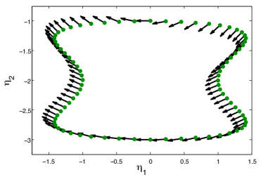
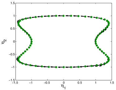
For illustrative purposes, Figure 2, we begin by applying our method to a simple example. We use one dimensional “dumbbell” manifold, with a regular sampling grid as recovering the density is quite straight forward density distribution in the form of a sinus of the circle. We exemplify a vector field that is not tangent to the manifold to show how the algorithm recovers only the tangiential component. The recovery of all three components is very good, even at this low sample size. As expected, only the tangential component of the vector field is recovered, as the normal component is unidentifyable from the diffusion process alone.

Figure 2: Artificial data of a one dimensional manifold sampled on a uniform grid with a smoothly varying vector field (left) and its recovery (right). The vector field has a component normal to the manifold, which cannot be recovered. The algorithm correctly recovers the tangential component of the vector field. we used $\epsilon=0.03$ and 400 sample points.

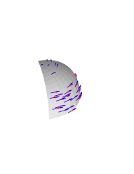
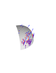
The next example is a 2 dimensional manifold. We experiment with 500 and 5000 sample points, and with two different vector fields, one of them with a normal component and one restricted to the tangent plane of $\mathcal{M}$. The sampling is non-uniform. Figure 3 shows only the vector field, for clarity. We see that even in the case of small sample size the recovery of $\mathbf{r}$ is remarkably accurate.

Figure 3: Spherical octant with non-uniform sampling and vector field $\mathbf{r}$ (in blue at 5% of the sampling points). The recovered $R$ is shown in red. Tangential$\mathbf{r}$ (left) and $\mathbf{r}$ with normal component (right). Recovery from 500 samples (top), respectively 5000 (bottom).

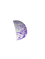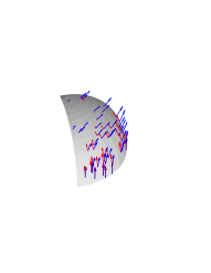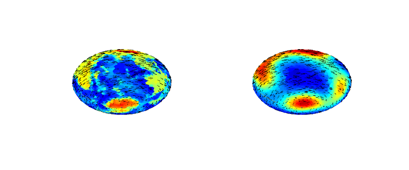
The final illustrative experiment considers the more involved example of a whole sphere with points sampled according to the Earth’s geographical map, with a vector field on it whose direction is tangent to the latitude curves. The embedding algorithm maps now to three dimensions.

Figure 4: Sphere with non-uniform map of sampling density and latitudinal vector field superimposed: model (left) and recovered components (right) from 4000 sample points with $\epsilon=0.01$.

5.2 Real Data

The National Longitudinal Survey of Youth (NLSY) followed a representative sample of young men and women in the United States from 1979 to 2000. This data was curated by , producing the data set we will refer to as Jobs.

The part of data set we use consists of a sample of 7,816 individual career sequences, of length 64, listing the jobs a particular individual held every quarter between the ages of 20 and 36. Each token in the sequence identifies a job as an industry $\times$ occupation pair. Approximately 213 distinct pairs occur in the data more than 50 times and we take these as our data set. They span 25 unique industry and 20 unique occupation indices. Thus, our graph has 213 nodes - the jobs - and our observations consist of 7,816 walks between the graph nodes.

We convert these walks to a directed graph with weigh matrix $A$, where $A_{ij}$ represents the number of times a transition from job $i$ to job $j$ was observed and setting the diagonal to 0. This latter step is motivated, in essence, by the observation that the “sticky” nature of jobs is an additional phenomenon, not modeled by our framework, and in fact largely independent of job type. Practically, we notice that small changes to the diagonal of $A$, e.g from 0 to 1, do not affect the final result significantly. Moreover, the removed diagonals can be preserved as a node attribute for further analysis. Note that this matrix is asymmetric, i.e $A_{ij}\neq A_{ji}$.

Figure 5: Embedding of Jobs along with estimated vector fields: total flow $\nabla U+\mathbf{r}$ (left) and $\mathbf{r}$ alone (right). The color map represents gender proportion (left, male = 0 and female = 1) and monthly wages in dollars (right).

With algorithm 1 we obtain an embedding of the job market that describes the relative position between jobs, their distribution, and the natural time progression from each job. From a purely statistical perspective, the embedding maps the “job” variable, a discrete variable with a very high number of possible values, to a much more manageable continuous variable. Besides the pragmatic advantages of the continuous parametrization w.r.t the discrete one, this model is highly plausible, as it is conceivable that jobs form a continuum, in which every encoding is a form of quantization. Our embedding algorithm is thus recovering the relative positions of the jobs in this continuum. Along with this, the natural time progression in jobs space is highly interesting.

Together, they summarize the job market dynamics by describing which jobs are naturally close as well as where they can lead in the future. From a public policy perspective, this can potentially address important questions such as which job may require extra attention in terms of helping individuals attain better upward mobility.

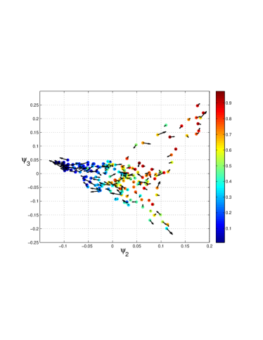
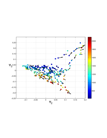
The job market was found to be a relatively high dimensional manifold, with about 10–12 eigevectors with significant eigenvalue. We present here only the dimensions that showed correlation with important demographic data, such as wages and gender. These were found to be coordinates 2 and 3, while other coordinates did not have a clear meaning. Figure 5 shows this two-dimensional sub-embedding along with the directional information for each dimension. We see the evident variation of gender along $\Psi_{2}$ and of wages along $\Psi_{3}$. The plots show a strong outward progression for most jobs, where outward progression is correlated to increasing wages.

To note that for describing the job dynamics, we are interested in the total advective flow, that sums the contributions of $\mathbf{r}$ and of diffusion, i.e $2(\nabla U+\mathbf{r})\cdot\nabla\phi$. It is easy to see that this flow can be obtained from $\mathcal{H}_{aa}^{(0)}-\mathcal{H}_{ss}^{(1)}$, or, in the matrix notation of Algorithm 1, as $(\Phi\Lambda-P\Phi)/2$. This is the vector field plotted in the left of Figure 5, while $\mathbf{r}$ alone is plotted on the right.

The temporal progression shown is explained by the natural diffusion process due to the non-uniform sampling density in job space, augmented with $\mathbf{r}$ which represents the other economic forces at work. From a policy-maker’s perspective, it is the latter term that matters, and that could be used for intervention, therefore $\mathbf{r}$ is depicted in Figure 5.

The embedding (left panel) suggests that males (blue) and females (red) tend to move away from each other over time, especially in the region of low-paying jobs, which seem to be specialized by gender. There is a particularly strong observed flow, mostly explain by the diffusion term, for men in low paying jobs to segregate towards more gender segregated, but slightly better paying jobs (e.g construction worker). One notices too a flow towards the lower corner, characterized by high paying jobs with equal proportions of men and women. The upper right corner of the embedding is occupied by women specific jobs. A few of these are high-paying (nurse). In this corner, a very strong $\mathbf{r}$ (flow explained by economic forces different than diffusion) leads from very low paying jobs towards the higher end jobs. It is to investigate if this shows that many women in low paying jobs, unlike the men in the same situation, are subject to some form of outside force towards upward mobility, but in reality (total flow) benefit little from it.

One notes also that the low-wage jobs away from the corners (in blue on the right panel) show little overall progression, while higher paid jobs seem to show some progression towards even better wages.

6 Discussion

From the theoretical point of view, we have introduced a generative model for directed graphs, in which the asymmetry is modeled explicitly as a vector field $\mathbf{r}$; this is a plausible and general model for digraphs. Moreover, we have shown that our representation for asymmetry is almost optimal, in the sense that representation that is more general is not identifiable from the data. This model is the first attempt to represent directed affinities with an infinitezimal generative model on a manifold

Second, with Theorem 1 we proved the continuous limit of a large class of operators based on asymmetric kernels. This is an original contribution onto itself.

As an example, our main theorem allowed us to derive the continuous limit of the WCut algorithm. The relationship between the WCut and this work parallels that between the MNCut of Shi and Malik (2000), and Coifman and Lafon (2006), Belkin and Niyogi (2002). The latter describe a generative process and operators that can be thought as the continous limits of the directed graph, random walk, graph Laplacian, and embedding algorithm. This paper performs the same analysis for the WCut algorithm as an embedding method for digraphs. Note too that that the WCut we use is similar to Zhou et al. (2005b). One could perform similar limit analyses based on Theorem 1 for other existing or novel directed embedding algorithms.

The theoretical results form the basis for a spectral algorithm that can be applied to a directed graph, to produce an embedding in a low-dimensional manifold, an estimate of the data density on the same manifold, and an estimate of the local directional flow at each point, which is the source of the graph’s asymmetry. As a byproduct of separating the asymmetry of the graph in the last feature, the directional flow, the geometry of the resulting manifold is identical to the one obtained by embedding a symmetric graph using the Diffusion Map algorithm of Coifman and Lafon (2006). We underscore that this property of our algorithm is not an ad-hoc choice, but a direct consequence of using a principled approach based on a generative model. Since the generative model for the embedding is the model proposed by Coifman and Lafon (2006), it is only natural that our algorithm recovers the same coordinates and sampling distribution as the Diffusion Map algorithm.

We have used from Coifman and Lafon (2006) the idea to renormalize the kernel (by $\alpha$) in order to be able to separate the density $p$ and the manifold geometry $\mathcal{M}$, and used some of the technical results developed there in our proofs. However, with respect to the asymmetric part of the kernel, everything starting from the defintion and the introduction of the vector field $\mathbf{r}$ as a way to model the asymmetry, through the derivation of the asymptotic expression for the symmetric and asymmetric kernel, is new. Regarding the use of renormalization, we go significantly beyond the elegant idea of Coifman and Lafon (2006) by analyzing the four different renormalizations possible for a given $\alpha$, each of them combining different aspects of $\mathcal{M},p$ and $\mathbf{r}$. Only the successful combination of two different renormalizations is able to recover the directional flow $\mathbf{r}$.

With respect to the previous work on directed graph embedding, several algorithms have been proposed for the embedding of directed graphs in low dimensional manifolds Pentney and Meilă (2005); Meila and Pentney (2007); Zhou et al. (2005b); Andersen et al. (2007). However, the analysis that relates a graph algorithm with a continuous generative model has not so far been attempted for directed graphs. In particular, the above methods do not explicitly attempt to separate the source of the asymmetry from the embedding. Hence, they only output a graph embedding, with no analog of the $\mathbf{r}$ estimate to explicitly account for the observed asymmetry. Therefore, just like in the embedding of undirected graphs, a non-uniform sampling density, if not accouted for explicitly, will confound the embedding coordinates, the unaccounted for asymmetry will appear in the embedding of the graph.

Ting et al. (2010) (THJ) presented asymptotic results for a general family of kernels that includes asymmetric and random kernels. Our $k_{\epsilon}$ can be expressed in the THJ notation by taking $w_{x}(y)\leftarrow 1+\mathbf{r}(x,y)\cdot(y-x)$, $r_{x}(y)\leftarrow 1$, $K_{0}\leftarrow h$, $h\leftarrow\epsilon$. The assumptions in TJH are more general than the assumptions we make here. However, THJ focus on the graph construction methods (seen as generative models for graphs), while we focus on explaining observed directed graphs through a manifold generative process. Moreover, while the THJ results can be used to analyze data from directed graphs, they differ from our Proposition 1. Specifically, with respect to the limit in Theorem 3 from THJ, we obtain the additional terms $f(x)\nabla\cdot\mathbf{r}$ and $c(x)f(x)$ in Theorem 1.

How general is our setup? The view of the graph nodes as sampled from a continuous manifold is standard in the machine learning spectral graph theory. However, for directed graphs, to the best of our knowledge, no one has before attempted to extend this generative model. In this respect the reader should note that our model of asymmetry is the most general possible, assuming the unidentifyable components of the $\mathbf{r}$ are set to fixed values. These are the component of $\mathbf{r}$ perpendicular to the manifold, whose effect is the function $c$ in Theorem 1, and a multiplicative constant for $\mathbf{r}$, resulting from the fact that the coordinate functions $\Phi$, as eigenvectors of the renormalized Laplacian $H^{(1)}_{ss}$, can only be recovered up to a multiplicative constant.

We note here that recovering $\mathbf{r}$ is just one, albeit the most useful, of the many ways of exploiting these theoretical resuls. For instance, one can also recover $\nabla\cdot\mathbf{r}$ directly, obtain the WCut embedding for $\alpha=0$, and check the consistency of the model on the real example at hand.

We foresee several other immediate applications of the framework developed here, like checking the model fit, estimating the dimension, parametrizations of the components $\mathcal{M},p,\mathbf{r}$ and so on. The practical applications are immediate, and we are currently applying this method to the analysis of the career sequences of section 5.2. Since the different coordinates of the manifold correlate well with demographic parameters like sex, wages, education, we expect that the different components of the vector field to be interpretable as social and personal forces that drive the individual carrer paths at different points in the job space.

Proof of the operator expansion (7)

The core of the proof is the asymptotic expansion of both $k_{\epsilon}$ and $f$ around a point $x\in\mathcal{M}$. In the same time we exploit the decay of the kernel $h_{\epsilon}$ with distance to approximate the integral over $\mathcal{M}$ with an integral over a ball around $x$ with radius of order $\sqrt{\epsilon}$. This allows for integrating the kernel over the tangent space $T\mathcal{M}_{x}$ at a given point $x\in\mathcal{M}$. Thus, the integration in (7) can be now changed from $\mathcal{M}$ to $\mathbb{R}^{d}$ because on a ball around $x$ where $\mathcal{M}$ can be approximated to $T\mathcal{M}_{x}$ (which is isomorphic to $\mathbb{R}^{d}$).

$$\int_{\mathcal{M}}k_{\epsilon}(x,y)f(y)dy\;=\;\int_{\mathbb{R}^{d}}k_{\epsilon}(x,x+(u,g(u)))\times$$

$$\left(\bar{f}(0)+\sum_{i=1}^{d}u_{i}\frac{\partial\bar{f}(0)}{\partial s_{i}}+\frac{1}{2}\sum_{i,j=1}^{d}u_{i}u_{j}\frac{\partial^{2}\bar{f}(0)}{\partial s_{i}\partial s_{j}}+\mathcal{Q}_{x,3}(u)\right)$$

$$\times\left(1+\mathcal{Q}_{x,2}(u)+\mathcal{Q}_{x,3}(u)\right)du+O(\epsilon^{2})\,.$$

In the derivation above, we used a number of asymptotic results of Coifman and Lafon (2006). We do not reproduce these here at length, as they can be found in Appendix B of Coifman and Lafon (2006). We now explain the origin of each of the terms in the expansion. The main idea is finding a natural set of coordinates to exploit the fact that the manifold $\mathcal{M}$ is locally flat.

The $s_{i}$’s are normal coordinates along geodesics of $\mathcal{M}$ that are defined by an orthonormal basis $(e_{1},...,e_{d})$ of the tangent space $T\mathcal{M}_{x}$. These coordinates serve to establish that the derivatives are taken along orthogonal geodesics of $\mathcal{M}$ at $x$, and so they can be used to define differential operators on $\mathcal{M}$ such as the Laplacian:

$$\Delta f(x)=\sum_{i=1}^{d}\frac{\partial^{2}\bar{f}(0)}{\partial s_{i}^{2}}\,.$$

Meanwhile, the $u_{i}^{\prime}s$ are the coordinates of $T\mathcal{M}_{x}$ in the $(e_{1},...,e_{d})$ basis. That is, they are determined by the projection of the manifold onto the $T\mathcal{M}_{x}$ by $u_{i}=(y-x)\cdot e_{i}$. The manifold is then locally parameterized by $y=x+(u,g(u))$ with $g:\mathbb{R}^{d}\rightarrow\mathbb{R}^{n-d}$ with $g(0)=0$ and $\frac{\partial g(0)}{\partial u_{i}}=0$ by construction. Finally, $\mathcal{Q}_{x,n}(u)$ denotes a polynomial in $u$ of order $n$ at $x$.

It remains to explain how two of the terms in (Proof of the operator expansion (7)) arise. The derivatives of $\bar{f}$ result from a Taylor expansion of $f(y)$ along the geodesics parametrized by the coordinates $(s_{1},...,s_{d})$. The Taylor expansion is then expressed in terms of the projected coordinates $u_{i}$ by making use of the fact that $s_{i}=u_{i}+\mathcal{Q}_{x,3}(u)+O(\epsilon^{2})$ (as the kernel radius is of the order $\sqrt{\epsilon}$ to bound the error by $\epsilon^{2}$ we need to go up to a third degree polynomial in the expansion). Meanwhile, the polynomial $1+\mathcal{Q}_{x,2}(u)+\mathcal{Q}_{x,3}(u)$ before the differential $du$ comes from the volume element of $\mathcal{M}$ at $y=x+(u,g(u))$. Specifically, it originates from the change of variable $y\rightarrow u$ given by $|det(dy/du)|=1+\mathcal{Q}_{x,2}(u)+\mathcal{Q}_{x,3}(u)$.

Next, we expand $k_{\epsilon}(x,x+(u,g(u)))$ in (Proof of the operator expansion (7)) in $u$. Dropping the terms that will be of order higher than $\epsilon$, we obtain:

$$h(||y-x||^{2}/\epsilon=h(||u||^{2}/\epsilon)+\frac{\mathcal{Q}_{x,4}(u)}{\epsilon}h^{\prime}(||u||^{2}/\epsilon)+O(\epsilon^{3/2})\,,$$ (25)

and

$$\mathbf{r}(x,y)\cdot(y-x)\,=\,$$

$$(\bar{r}(x,0)+\sum_{i=1}^{d}u_{i}\frac{\partial\bar{r}(x,0)}{\partial s_{i}})\cdot(u,\sum_{i,j=1}^{d}\frac{u_{i}u_{j}}{2}\frac{\partial^{2}g(0)}{\partial u_{i}\partial u_{j}})+O(\epsilon^{2})\,.$$

As mentioned before, $\mathbf{r}(x,y)$ is taken here to represent a vector field on $\mathcal{M}$. To make sense of this interpretation, we note that the $y$ variable is important only in a ball of radius $\epsilon^{1/2}$ around $x$ because of the form of $h_{\epsilon}(x,y)$, and that only the linear term in the expansion of $\mathbf{r}(x,y)$ is important. If we impose that $\nabla_{x}\mathbf{r}(x,y)|_{y=x}=\nabla_{y}\mathbf{r}(x,y)|_{y=x}$, it follows that the kernel “sees” locally in the same vector field as the global vector field $\mathbf{r}(x,x)$ defined on $\mathcal{M}$.

Substituting (25) and (Proof of the operator expansion (7)) into (Proof of the operator expansion (7)) and integrating finishes the proof.

The first two terms in (1), $\omega(x)f(x)$ and $\Delta f(x)$, come from the symmetric kernel $h_{\epsilon}(x,y)$. $\Delta f(x)$ comes from

$$\sum_{i,j=1}^{d}\int_{\mathbb{R}^{d}}u_{i}u_{j}\frac{\partial^{2}\bar{f}(0)}{\partial s_{i}\partial s_{j}}\frac{h(||u||^{2}/\epsilon)}{\epsilon^{d/2}}du\,=\,\epsilon\Delta f(x)\,,$$

where all the off-diagonal terms in the sum vanish because the kernel was chosen to be radially symmetric. Meanwhile, $\omega(x)f(x)$ is a geometric effect of the manifold $\mathcal{M}$, as it embodies the effect of the manifold on the kernel and the change in volume element. As this term ultimately cancels out, it will not be further discussed.

The remaining terms are all contributions from the asymmetric part of the kernel. The $\mathbf{r}\cdot\nabla f(x)$ term comes from the kernel picking up transport induced by the vector field $\mathbf{r}(x)=\mathbf{r}(x,x)$

$$\epsilon\mathbf{r}\cdot\nabla f(x)=\sum_{i,j=1}^{d}r_{i}\int_{\mathbb{R}^{2}}u_{i}u_{j}\frac{\partial\bar{f}(0)}{\partial s_{j}}\frac{h(||u||^{2}/\epsilon)}{\epsilon^{d/2}}du\,,$$

while $f(x)\nabla\cdot\mathbf{r}$ comes from the kernel augmenting or reducing $f(x)$ by the amount of divergence of the vector field

$$\epsilon f(x)\nabla_{z}\cdot\mathbf{r}(z,x)|_{z=x}\,=\,$$

$$\sum_{i,j=1}^{d}\int_{\mathbb{R}^{2}}u_{i}u_{j}\frac{\partial\bar{r_{j}}(x,s)}{\partial s_{i}}|_{s=0}\times\frac{h(||u||^{2}/\epsilon)}{\epsilon^{d/2}}du\,,$$

where we have implicitly made use of the fact that $r$ is assumed to satisfy $\nabla_{x}\mathbf{r}(x,y)|_{y=x}=\nabla_{y}\mathbf{r}(x,y)|_{y=x}$. The remaining term, $c(x)f(x)$, arises if the vector field $\mathbf{r}(x)$ has a component perpendicular to $T\mathcal{M}_{x}$ at a point where the orientation of $T\mathcal{M}_{x}$ is changing:

$$\epsilon f(x)c(x)=\sum_{i,j,k=1}^{d}r_{k}\int_{\mathbb{R}^{2}}u_{i}u_{j}\frac{\partial^{2}g_{k}(0)}{\partial u_{i}\partial u_{j}}\frac{h(||u||^{2}/\epsilon)}{\epsilon^{d/2}}du\,.$$

References

- Andersen et al. (2007) Reid Andersen, Fan R. K. Chung, and Kevin J. Lang. Local partitioning for directed graphs using pagerank. In WAW, pages 166–178, 2007.
- Belkin and Niyogi (2002) Belkin and Niyogi. Laplacian eigenmaps for dimensionality reduction and data representation. Neural Computation, 15:1373–1396, 2002.
- Coifman and Lafon (2006) Coifman and Lafon. Diffusion maps. Applied and Computational Harmonic Analysis, 21:6–30, 2006.
- Coifman et al. (2005) Coifman, Lafon, Lee, Maggioni, Warner, and Zucker. Geometric diffusions as a tool for harmonic analysis and structure definition of data: Diffusion maps. In Proceedings of the National Academy of Sciences, pages 7426–7431, 2005.
- Hoff et al. (2002) Hoff, Raftery, and Handcock. Latent space approaches to social network analysis. Journal of the American Statistical Association, 97:1090–1098, 2002.
- Meila and Pentney (2007) Meila and Pentney. Clustering by weighted cuts in directed graphs. In SIAM Data Mining Conference, 2007.
- Meilă and Shi (2001) Marina Meilă and Jianbo Shi. A random walks view of spectral segmentation. In T. Jaakkola and T. Richardson, editors, Artificial Intelligence and Statistics AISTATS, 2001.
- Nadler et al. (2006a) Nadler, Lafon, and Coifman. Diffusion maps, spectral clustering and eigenfunctions of fokker-planck operators. In Neural Information Processing Systems Conference, 2006a.
- Nadler et al. (2006b) Nadler, Lafon, Coifman, and Kevrekidis. Diffusion maps, spectral clustering and reaction coordiantes of dynamical systems. Applied and Computational Harmonic Analysis, 21:113–127, 2006b.
- Pentney and Meilă (2005) William Pentney and Marina Meilă. Spectral clustering of biological sequence data. In Manuela Veloso and Subbarao Kambhampati, editors, Proceedings of Twentieth National Conference on Artificial Intelligence (AAAI-05), pages 845–850, Menlo Park, California, 2005. The AAAI Press.
- Shi and Malik (2000) Jianbo Shi and Jitendra Malik. Normalized cuts and image segmentation. PAMI, 2000.
- Ting et al. (2010) Ting, Huang, and Jordan. An analysis of the convergence of graph Laplacians. In International Conference on Machine Learning, 2010.
- Zhou et al. (2005a) Zhou, Huang, and Scholkopf. Learning from labeled and unlabeled data on a directed graph. In International Conference on Machine Learning, pages 1041–1048, 2005a.
- Zhou et al. (2005b) Zhou, Schoelkopf, and Hofmann. Semi-supervised learning on directed graphs. In Advances in Neural Information Processing Systems, volume 17, pages 1633–1640, 2005b.