Hairy black holes: stability under odd-parity perturbations and existence of slowly rotating solutions

Abstract

We show that, independently of the scalar field potential and of specific asymptotic properties of the spacetime (asymptotically flat, de Sitter or anti-de Sitter), any static, spherically symmetric or planar, black hole or soliton solution of the Einstein theory minimally coupled to a real scalar field with a general potential is mode stable under linear odd-parity perturbations. To this end, we generalize the Regge-Wheeler equation for a generic self-interacting scalar field, and show that the potential of the relevant Schrödinger operator can be mapped, by the so-called S-deformation, to a semi-positively defined potential. With these results at hand we study the existence of slowly rotating configurations. The frame dragging effect is compared with the Kerr black hole.

1 Introduction

In the light of discoveries of last decades like cosmic acceleration, associated with “dark energy”, or more definitive indications of the existence of “dark matter”, Einstein’s classical general relativity has occurred again “on the firing line”, to use Cliff Will’s metaphor from the October 1972 issue of Physics Today. Numerous modifications of Einstein’s theory assume the existence of scalar field(s). Scalar fields are part of the inflationary paradigm and appear conspicuously in string theory and supergravity. The reality of a fundamental scalar field appears to be supported by the discovery of the Brout-Englert-Higgs boson. The interest on the interaction of scalar fields and gravity is however older than inflation and supergravity and can be traced back to the well known Brans-Dicke theory and the black hole no-hair theorems. The original, and well known, no-hair theorem of Bekenstein states that a convex potential is incompatible with the existence of a static black hole in asymptotically flat spacetime [1]. This is also supported by the fact that massive scalar fields develop a power-law singularity at the horizon when solved in the Kerr-Newman background [2]. Bekenstein’s theorem was generalized and we understand now that the relevant requirement for an asymptotically flat black hole to exist in the presence of a regular, non-trivial, scalar field profile is the existence of a negative region of the scalar field potential [3, 4].

An interest has been revived in black holes in scalar-tensor theories and their perturbations; for solutions with a real minimally coupled scalar field, see [5]; for solutions in theories with non-minimal derivative coupling, see [6]; for stability, see [7]. In particular, a Japanese group studied black hole perturbations in a general gravitational theory with Lagrangian given by an arbitrary function of the Ricci scalar and the Chern-Simons pseudoinvariant [8, 9]. Most recently, the authors associated with this group tackled a technically involved problem of perturbations of black holes in the most general scalar-tensor theory in which all field equations are of the second order. Their Lagrangian includes, for example, the Brans-Dicke theory, $f(R)$ gravity, the non-minimal coupling to the Gauss-Bonnet term, etc. The odd-parity perturbations have been tackled first [10]; most recently, the even-parity sector was also analyzed [11]. The authors concentrate primarily on deriving perturbation equations from the second-order actions. In both cases they present general conditions, necessary but not sufficient, for the (gradient) stability of a static, spherically symmetric solution.

We remain in the framework of classical four dimensional general relativity and consider perturbations and stability of static, spherically symmetric, planar and hyperbolic hairy black holes in asymptotically flat or asymptotically (anti-) de Sitter spacetimes in which a scalar field is minimally coupled to gravity (for a recent review, see [12]). Then we analyze their odd-parity perturbations following the general treatment of the “axial” perturbations of spherically symmetric (not necessarily vacuum) spacetimes by Chandrasekhar [13]. We prove the mode stability with respect to general perturbations in the odd-parity sector.

Very recently, Bhattacharya and Maeda [14] arrived at a conclusion, based on the slow-rotation approximation, that Bocharova-Bronnikov-Melnikov-Bekenstein black hole [15, 16] with a scalar field coupled conformally to gravity cannot rotate (for related discussions se also [17, 18, 19]). We provide examples when the rotation of a general class of hairy black holes is admissible. Although in the odd-parity case, the gravitational perturbations are fully decoupled from the scalar field perturbations, they can strongly be influenced by the background scalar field. The situation resembles general perturbations of charged (Reissner-Nordström) black holes where the background electric field influences gravitational perturbations (cf. [20, 21, 22]). The right-hand side of Einstein’s equations is given in terms of the energy-momentum tensor of (possibly strong) background scalar field and odd-parity perturbations of the metric. As a consequence, the metric component like $g_{\varphi t}$, which implies the dragging of inertial frames outside a rotating black hole, depends on the character of the background scalar field. We illustrate this effect.

Rotating black holes and boson stars are known to exist when a complex scalar field is minimally coupled to Einstein theory [23]. However, much less is known when the scalar field is real. To construct the slowly rotating solutions it is necessary to specify the background. Thus, we use the static black hole family originally found in [24]. This family of solutions is the most general four dimensional hairy black hole family with a single real scalar field and contains all other exact black holes available in the literature. The details can be found in [12].

The outline of this article is as follows. In the second section we present the proof that for minimally coupled scalar fields with arbitrary self-interaction, the spectrum of the generalized Regge-Wheeler equation is always positive. The proof is done in detail for spherical geometries and generalized to planar trasnversal geometries. The third section introduces the perturbative frame-dragging computation for the hairy black hole. We briefly describe the hairy black hole geometries before comparing the frame draging effect with the Kerr black hole. Finally we present a discussion of our main results. Our conventions are such that the Riemann tensor and the Ricci scalar of a sphere are positive in an orthonormal basis. The metric signature is $(-,+,+,+)$ and we set $\kappa=8\pi G$, $c=1$.

2 Odd-parity perturbations and generalized Regge-Wheeler equation

Here we follow closely [13]. We shall consider a minimally coupled real scalar field with an arbitrary potential, $V(\phi)$. The field equations are

$$E_{\mu\nu} \equiv G_{\mu\nu}-\kappa T_{\mu\nu}=0\text{ },$$ (1)

$$T_{\mu\nu} =\partial_{\mu}\phi\partial_{\nu}\phi-g_{\mu\nu}\left[\frac{1}{2}\left(\partial\phi\right)^{2}+V(\phi)\right]\ ,$$ (2)

where $G_{\mu\nu}$ is the Einstein tensor and a possibly non-vanishing consmological constant can be included in $V(\phi)$. The perturbed metric reads

$$ds^{2}=-A(r)dt^{2}+B(r)dr^{2}+C(r)\left[\frac{dz^{2}}{\left(1-kz^{2}\right)}+\left(1-kz^{2}\right)\left(d\varphi+k_{1}dt+k_{2}dr+k_{3}dz\right)^{2}\right]\ ,$$ (3)

where $k_{1}$, $k_{2}$ and $k_{3}$ are functions of ($t,r,z$). $A(r),$ $B(r)$ and $C(r)$ are the metric functions parameterizing the most general static background solution of a scalar-tensor theory. For asymptotically locally AdS solutions $k=\pm 1\,\$or $0$ [25]. Asymptotically flat or de Sitter solutions have $k=1$. The scalar field is taken to be of the form

$$\phi=\phi_{0}(r)+\epsilon\Phi\left(t,r,z\right)\ ,$$ (4)

where $\phi_{0}$ is the background field. The metric perturbations $\left(k_{1},k_{2},k_{3}\right)$ are all taken to be first order in $\epsilon$. Since any surface of constant $(t,r)$ is of constant curvature, we consider only axisymmetric perturbations, without any loss of generality (for more details of the spherically symmetric case, see [13]). The Einstein field equations are truncated at first order in $\epsilon$. This yields the vanishing of $\Phi$. Indeed, using the notation introduced in equation (1) and the zeroth-order (background) equations we find that

$$E_{r}^{t} =\epsilon\kappa\frac{d\phi_{0}}{dr}\frac{\partial_{t}\Phi}{A(r)}+O(\epsilon^{2})=0\text{ },$$ (5)

$$E_{z}^{r} =-\epsilon\kappa\frac{d\phi_{0}}{dr}\frac{\partial_{z}\Phi}{B(r)}+O(\epsilon^{2})=0\text{ },$$ (6)

$$E_{t}^{t} =\frac{\epsilon\kappa}{B(r)}\left(\frac{d\phi_{0}}{dr}\partial_{r}\Phi+BV_{1}\Phi\right)+O(\epsilon^{2})=0\text{ },$$ (7)

where $V_{1}$ arises from the expansion of the scalar field potential around the background configuration,

$$V_{1}=\left.\frac{dV}{d\phi}\right|_{\phi=\phi_{0}}\text{ }.$$ (8)

Equations (5)-(7) imply that $\partial_{t}\Phi=0=\partial_{z}\Phi$ and $\frac{d\phi_{0}}{dr}\partial_{r}\Phi=-BV_{1}\Phi$. This information simplifies equation for $E_{r}^{r}:$

$$E_{r}^{r}=2\epsilon\kappa V_{1}\Phi+O(\epsilon^{2})=0\text{ }.$$ (9)

Thus, it follows that $\Phi=0$. Using the zeroth-order equations, it is possible to check that the remaining equations are satisfied up to linear order in $\epsilon$ if the following system of equations is satisfied:

$$\frac{\partial}{\partial r}\left[C\sqrt{\frac{A}{B}}\left(\partial_{z}k_{2}-\partial_{r}k_{3}\right)\right]+\frac{\partial}{\partial t}\left[C\sqrt{\frac{B}{A}}\left(\partial_{t}k_{3}-\partial_{z}k_{1}\right)\right] =0\text{ },$$ (10)

$$\frac{\partial}{\partial z}\left[\frac{A}{C}(1-kz^{2})^{2}\left(\partial_{z}k_{2}-\partial_{r}k_{3}\right)\right]+\frac{\partial}{\partial t}\left[(1-kz^{2})\left(\partial_{r}k_{1}-\partial_{t}k_{2}\right)\right] =0\text{ },$$ (11)

$$\frac{\partial}{\partial z}\left[C\sqrt{\frac{B}{A}}(1-kz^{2})^{2}\left(\partial_{z}k_{1}-\partial_{t}k_{3}\right)\right]+\frac{\partial}{\partial r}\left[(1-kz^{2})\frac{C^{2}}{\sqrt{AB}}\left(\partial_{r}k_{1}-\partial_{t}k_{2}\right)\right] =0\text{ }.$$ (12)

Introducing the variable $Q=CA^{1/2}B^{-1/2}(1-kz^{2})^{2}\left(\partial_{z}k_{2}-\partial_{x}k_{3}\right)$, equations (10)-(11) yield

$$\frac{A^{1/2}}{CB^{1/2}\left(1-kz^{2}\right)^{2}}\frac{\partial Q}{\partial r} =-\partial_{t}^{2}k_{3}+\partial_{t}\partial_{z}k_{1}\text{ },$$ (13)

$$\frac{\sqrt{AB}}{C^{2}}\frac{1}{\left(1-kz^{2}\right)}\frac{\partial Q}{\partial z} =-\partial_{t}\partial_{r}k_{1}+\partial_{t}^{2}k_{2}\text{ }.$$ (14)

The combination $\partial_{r}$(13)+$\partial_{z}$(14) can be written in terms of $Q,$

$$\frac{C^{2}}{\sqrt{AB}}\frac{\partial}{\partial r}\left[\frac{A^{1/2}}{CB^{1/2}}\frac{\partial Q}{\partial r}\right]+(1-kz^{2})^{2}\frac{\partial}{\partial z}\left[\frac{1}{\left(1-kz^{2}\right)}\frac{\partial Q}{\partial z}\right]=\frac{C}{A}\partial_{t}^{2}Q\text{ }.$$ (15)

This equation can be solved by separation of variables. Writting $Q=q(r,t)D(z),$ we obtain:

$$\frac{C^{2}}{\sqrt{AB}}\frac{\partial}{\partial r}\left[\frac{A^{1/2}}{CB^{1/2}}\frac{\partial Q}{\partial r}\right]-\lambda Q =\frac{C}{A}\partial_{t}^{2}Q\text{ },$$ (16)

$$\left(1-kz^{2}\right)^{2}\frac{\partial}{\partial z}\left[\frac{1}{\left(1-kz^{2}\right)}\frac{\partial D}{\partial z}\right] =-\lambda D\text{ }.$$ (17)

Let us now concentrate on the case with $k=1$; we shall briefly comment on the other cases later. Setting $z=\cos\theta$ in equation (17) allows to identify $C_{l+2}^{-3/2}(\theta)=D(z)$ with a Gegenbauer polynomial with $\lambda=\left(l-1\right)\left(l+2\right)$ where $l\geq 1$ holds. The master variable in this case is $\Psi(r^{\ast},t)=q(r,t)C^{-1/2}$ where $\frac{\partial}{\partial r}=\frac{B^{1/2}}{A^{1/2}}\frac{\partial}{\partial r^{\ast}}$. Inserting all this information in equation (16) yields the master equation

$$\frac{\partial^{2}\Psi}{\partial r^{\ast 2}}+\left(\frac{1}{2C}\frac{d^{2}C}{dr^{\ast 2}}-\frac{3}{4C^{2}}\left(\frac{dC}{dr^{\ast}}\right)^{2}-\lambda\frac{A}{C}\right)\Psi=\partial_{t}^{2}\Psi\text{ }.$$ (18)

The mode stability can be studied using the Fourier decomposition of the master variable, $\Psi=\int\Psi_{\omega}e^{i\omega t}dt$, which yields

$$\mathcal{H}\Psi_{\omega}\equiv-\frac{d^{2}\Psi_{\omega}}{dr^{\ast 2}}+\left(\lambda\frac{A}{C}+\frac{3}{4C^{2}}\left(\frac{dC}{dr^{\ast}}\right)^{2}-\frac{1}{2C}\frac{d^{2}C}{dr^{\ast 2}}\right)\Psi_{\omega}=\omega^{2}\Psi_{\omega}\text{ }.$$ (19)

The scalar field perturbation vanishes, however equation (19) depends on the background scalar field through its influence on the background metric. In vacuum, $A=1-2m/r$, $C=r^{2}$, and equation (19) becomes the Regge-Wheeler equation. The operator $\mathcal{H}$ is not manifestly positive, however, its spectrum is positively defined as follows from

$$\int dr^{\ast}\left(\Psi_{\omega}\right)^{\ast}\mathcal{H}\Psi_{\omega}=\int dr^{\ast}\left[\left|D\Psi_{\omega}\right|^{2}+V_{S}\left|\Psi_{\omega}\right|^{2}\right]-\left.\left(\Psi_{\omega}D\Psi_{\omega}\right)\right|_{Boundary}\text{ },$$ (20)

where $D=\frac{d}{dr^{\ast}}+S$ and

$$V_{S}=\lambda\frac{A}{C}+\frac{3}{4C^{2}}\left(\frac{dC}{dr^{\ast}}\right)^{2}-\frac{1}{2C}\frac{d^{2}C}{dr^{\ast 2}}+\frac{dS}{dr^{\ast}}-S^{2}\text{ }.$$ (21)

Choosing $S=\frac{1}{2C}\frac{dC}{dr^{\ast}},$ we find

$$V_{S}=\lambda\frac{A}{C}\text{ }.$$ (22)

Therefore $l\geq 1\Longrightarrow\lambda\geq 0\Longrightarrow V_{S}\geq 0$ whenever $A>0$, namely in any static region of the spacetime. From equations (20-22) it follows that all the spherically symmetric four dimensional hairy configurations are mode stable under odd-parity perturbations. To reach this conclusion it is necessary that

$$\left.\left(\Psi_{\omega}D\Psi_{\omega}\right)\right|_{Boundary}=0\text{ },$$ (23)

which requires that the perturbation vanishes at the horizon. This is not a very strong requirement, as follow from [27]; linear stability under the boundary condition $\Psi=0$ at the horizon implies stability under boundary conditions with $\Psi$ taking a finite value at the horizon.

Note that $k\,$ goes into the perturbation equation (19) only through $\lambda\,$. When $k=0$ the requirement that the perturbations are everywhere well defined is satisfied only if $\lambda>0$ which implies $V_{S}\geq 0$. The equation for the angular part is just the equation for the harmonic oscillator with frequency $\sqrt{\lambda}$. When $k=-1,$ further analysis is required.

3 Slowly rotating hairy black holes

Here we want to establish the existence of slowly rotating hairy black holes. To this end we shall consider only stationary perturbations with $k_{2}=k_{3}=0$ and $k_{1}=\omega(r)$. In this case equation (12) yields

$$\omega=-c_{1}\int\frac{\sqrt{AB}}{C^{2}}dr+c_{2}\text{ },$$ (24)

where $c_{1}$ and $c_{2}$ are two integration constants. To warm up, let us consider now the case of the Schwarzschild black hole. We have $\sqrt{AB}=1$ and $C=r^{2},$ so it follows that

$$\omega=\frac{c_{1}}{3r^{3}}+c_{2}\text{ }.$$ (25)

Hence, choosing $c_{2}=0$ and $c_{1}=3Ma,$ we find that the perturbed metric is the Schwarzschild metric plus the perturbation $g_{t\varphi}=\frac{Ma(1-z^{2})}{r}$ which, when terms proportional to $a^{2}$ are neglected, coincides exactly with the Kerr metric in the Boyer-Lindquist coordinates.

Now let us consider the hairy black hole family [12, 24]. The following configurations are exact background solutions of the Einstein equations (1):

$$ds^{2}=\Omega(x)\left[-f(x)dt^{2}+\frac{\eta^{2}dx^{2}}{f(x)}+\frac{dz^{2}}{1-kz^{2}}+\left(1-kz^{2}\right)d\varphi^{2}\right]\text{ ,}$$ (26)

$$\Omega(x)=\frac{\nu^{2}x^{\nu-1}}{\eta^{2}\left(x^{\nu}-1\right)^{2}}\text{ },$$ (27)

$$f(x)=\frac{x^{2-\nu}\left(x^{\nu}-1\right)^{2}\eta^{2}k}{\nu^{2}}+\left(\frac{1}{\nu^{2}-4}-\frac{x^{2}}{\nu^{2}}\left(1+\frac{x^{-\nu}}{\nu-2}-\frac{x^{\nu}}{\nu+2}\right)\right)\alpha+\frac{1}{l^{2}}\text{ ,}$$ (28)

with energy-momentum tensor given by equation (2), scalar field potential and background scalar field by:

$$V(\phi) =\frac{\alpha}{\kappa\nu^{2}}\left[\frac{\nu-1}{\nu+2}\sinh(\phi l_{\nu}\left(\nu+1\right))-\frac{\nu+1}{\nu-2}\sinh(\phi l_{\nu}\left(\nu-1\right))+4\frac{\nu^{2}-1}{\nu^{2}-4}\sinh(\phi l_{\nu})\right]$$

$$-\frac{\left(\nu^{2}-4\right)}{2\kappa l^{2}\nu^{2}}\left[\frac{\nu-1}{\nu+2}\exp(-\phi l_{\nu}\left(\nu+1\right))+\frac{\nu+1}{\nu-2}\exp(\phi l_{\nu}\left(\nu-1\right))+4\frac{\nu^{2}-1}{\nu^{2}-4}\exp(-\phi l_{\nu})\right]\text{ ,}$$ (29)

and

$$\phi_{0}=l_{\nu}^{-1}\ln x\text{ ,}$$ (30)

where parameter $\eta$ is the unique integration constant; it arises in a non-standard form which allows to write the solution in terms of a dimensionless radial coordinate $x$ and $l_{\nu}^{-1}=\sqrt{\frac{\nu^{2}-1}{2\kappa}\text{. }}$The metric and the potential are invariant under the change $\nu\rightarrow-\nu$, therefore, it is possible to take $\nu\geq 1$. Furthermore, it should be noted that the asymptotic region is at $x=1$ which can be seen from the pole of order two in $\Omega(x)$. There are two solutions, depending on whether the scalar field is negative, $x\in(0,1),$ or positive, $x\in(1,\infty),$ which allows to cover all the values of the scalar field potential. The metric is regular for any value of $x\neq 0$ and $x\neq\infty$ as can be seen from the introduction of advanced and retarded coordinates, $u_{\pm}=t\mp\int\frac{\eta}{f(x)}dx$. The scalar field and the geometries are singular at $x=0$ and $x=\infty$ but these singularities can be covered by event horizons. The metric reduces to the Schwarzschild-(A)dS solution in Schwarzschild-Droste coordinates when $\nu=1$ and setting $x=1\pm 1/\left(\eta r\right)$. The mass of the spherically symmetric solution, computed with the Hamiltonian method [28], yields

$$M=\pm\frac{\alpha+3\eta^{2}}{6\eta^{3}G}\text{ .}$$ (31)

where the $\pm$ depends on whether one is considering the branch where $x>1$ or $x<1$.

In analogy with the Kerr solution, the slowly rotating hairy black hole is a deformation of the static one plus $g_{t\varphi}=\omega_{\nu}(1-z^{2})\Omega(x).$ The metric component $g_{t\varphi}$ determines the frame dragging potential (see e.g. [29] Ex. 3.4). We find that

$$\omega_{\nu}=\bar{c}_{1}\frac{x^{2-\nu}}{\nu^{2}(\nu^{2}-4)}(\left(\nu-2\right)x^{2\nu}+\left(4-\nu^{2}\right)x^{\nu}-2-\nu)+\bar{c}_{2}\text{ ;}$$ (32)

requiring that $\omega_{\nu}(x=1)=0$ fixes $\omega$ up to an overall multiplicative constant,

$$\omega_{\nu}=\bar{c}_{1}\left(\frac{x^{2-\nu}}{\nu^{2}(\nu^{2}-4)}(\left(\nu-2\right)x^{2\nu}+\left(4-\nu^{2}\right)x^{\nu}-2-\nu)+\frac{1}{\nu^{2}-4}\right)\text{ .}$$ (33)

To measure the deviation from the slowly rotating Kerr solution we plot the ratio $\omega/\omega_{\nu=1}$ versus the square root of the areal function $\sqrt{\Omega(x)}$. The integration constant $\eta$ has units of inverse of length squared. Hence the $x$-axis is measured in units of $\eta^{-1}$ (e.g. km, parsec, etc.). In Figure 1 it can be seen that there is a smooth departure from the Kerr frame dragging as both coincide when $\nu$ approaches 1 as well as asymptotically for large $\sqrt{\Omega(x)}$. It should be noticed that the departure from Kerr can be important and that the horizon can be located at any point in the graph. Indeed, the location of the horizon is defined by the equation $f(x_{+})=0$, which has solution for any $x_{+}$ by adjusting the value of $\alpha$ in expression (28).

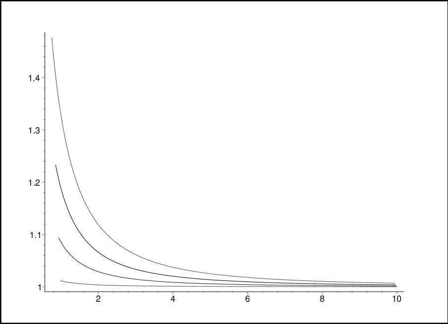
Figure 1: The ratio $\omega/\omega_{\nu=1}$ versus the square root of the areal function, $\sqrt{\Omega(x)}$, for different values of $\nu$. The plots are for $\nu=1.2,\nu=2.1,\nu=3$ and $\nu=4$ (from down up).

4 Conclusions

In this paper we addressed the issue of odd-mode stability in a rather general class of scalar-tensor theories. We proved that for a minimally-coupled real scalar field, independently of its self-interaction and of the asymptotic properties of the spacetime (asymptotically flat, de Sitter or anti-de Sitter), any static soliton or black hole solution is mode stable under these perturbations. The situation is such that the scalar field only contributes through the backreaction of the background solution and the dynamics is dictated by the linearized Einstein equations. This is in contrast of what happens with the spherically symmetric mode where the only propagating mode is the scalar one [7]. The linearized Einstein-scalar field equations allowed us to study the existence of slowly rotating hairy black hole solutions. Using the hairy black hole family [12, 24], we have shown that there is no obstruction for the existence of rotating hairy black holes and that they can have a behavior that strongly departs from the Kerr solution. Indeed, it would be very interesting to study the even modes outside the spherically symmetric regime, namely when the scalar and the tensor perturbations interact non-trivially. We leave this question open to further research.

5 Acknowledgments

Research of A.A. is supported in part by the Fondecyt Grants N^o 11121187, 1141073. Research of J.S. is supported in part by the Fondecyt Grants N^o 1110076, 1110230. J.B. acknowledges the support from CONICYT and is grateful for a wonderful hospitality offered by colleagues at Ponitificia Universidad Catolica de Valparaiso, Universidad Adolfo Ibañez de Viña del Mar and Universidad Andres Bello de Santiago. J.B. acknowledges the support from the Czech Science Foundation, grant N^o 14-37086G (Albert Einstein Center).

References

- [1] J. D. Bekenstein, “Nonexistence of baryon number for static black holes,” Phys. Rev. D 5 (1972) 1239. J. D. Bekenstein, “Novel ’no scalar hair’ theorem for black holes,” Phys. Rev. D 51 (1995) 6608.
- [2] J. Bičák, Z. Stuchlík and M. Šob, “Scalar Fields Around a Charged, Rotating Black Hole,” Czech. J. Phys. B 28 (1978) 121.
- [3] M. Heusler, “A No hair theorem for selfgravitating nonlinear sigma models,” J. Math. Phys. 33 (1992) 3497.
- [4] D. Sudarsky, “A Simple proof of a no hair theorem in Einstein Higgs theory,,” Class. Quant. Grav. 12 (1995) 579.
- [5] T. Torii, K. Maeda and M. Narita, “Scalar hair on the black hole in asymptotically anti-de Sitter space-time,” Phys. Rev. D 64 (2001) 044007. D. Sudarsky and J. A. Gonzalez, “On black hole scalar hair in asymptotically anti-de Sitter space-times,” Phys. Rev. D 67, 024038 (2003) [gr-qc/0207069] U. Nucamendi and M. Salgado, “Scalar hairy black holes and solitons in asymptotically flat space-times,” Phys. Rev. D 68, 044026 (2003) [gr-qc/0301062]. T. Hertog and K. Maeda, “Black holes with scalar hair and asymptotics in N = 8 supergravity,” JHEP 0407 (2004) 051 [hep-th/0404261]. C. Martinez, R. Troncoso and J. Zanelli, “Exact black hole solution with a minimally coupled scalar field,” Phys. Rev. D 70 (2004) 084035 [hep-th/0406111]. K. G. Zloshchastiev, “On co-existence of black holes and scalar field,” Phys. Rev. Lett. 94 (2005) 121101 [hep-th/0408163]. A. Anabalon, F. Canfora, A. Giacomini and J. Oliva, “Black Holes with Primary Hair in gauged N=8 Supergravity,” JHEP 1206 (2012) 010 [arXiv:1203.6627 [hep-th]]. A. Anabalon and J. Oliva, “Exact Hairy Black Holes and their Modification to the Universal Law of Gravitation,” Phys. Rev. D 86 (2012) 107501 [arXiv:1205.6012 [gr-qc]]. C. Toldo and S. Vandoren, “Static nonextremal AdS4 black hole solutions,” JHEP 1209 (2012) 048 [arXiv:1207.3014 [hep-th]]. A. Acena, A. Anabalon and D. Astefanesei, “Exact hairy black brane solutions in and holographic RG flows,” Phys. Rev. D 87 (2013) 12, 124033 [arXiv:1211.6126 [hep-th]]. J. Aparicio, D. Grumiller, E. Lopez, I. Papadimitriou and S. Stricker, “Bootstrapping gravity solutions,” JHEP 1305 (2013) 128 [arXiv:1212.3609 [hep-th]]. B. Kleihaus, J. Kunz, E. Radu and B. Subagyo, “Axially symmetric static scalar solitons and black holes with scalar hair,” Phys. Lett. B 725 (2013) 489 [arXiv:1306.4616 [gr-qc]]. P. A. González, E. Papantonopoulos, J. Saavedra and Y. Vásquez, “Four-Dimensional Asymptotically AdS Black Holes with Scalar Hair,” JHEP 1312 (2013) 021 [arXiv:1309.2161 [gr-qc]]. A. Acena, A. Anabalon, D. Astefanesei and R. Mann, “Hairy planar black holes in higher dimensions,” JHEP 1401 (2014) 153 [arXiv:1311.6065 [hep-th]]. A. Anabalon and D. Astefanesei, “Black holes in -defomed gauged supergravity,” arXiv:1311.7459 [hep-th]. X. -H. Feng, H. Lu and Q. Wen, “Scalar Hairy Black Holes in General Dimensions,” Phys. Rev. D 89 (2014) 044014 [arXiv:1312.5374 [hep-th]]. H. -S. Liu and H. Lü, “Scalar Charges in Asymptotic AdS Geometries,” Phys. Lett. B 730 (2014) 267 [arXiv:1401.0010 [hep-th]].
- [6] T. Kolyvaris, G. Koutsoumbas, E. Papantonopoulos and G. Siopsis, “Scalar Hair from a Derivative Coupling of a Scalar Field to the Einstein Tensor,” Class. Quant. Grav. 29 (2012) 205011 [arXiv:1111.0263 [gr-qc]]. M. Rinaldi, “Black holes with non-minimal derivative coupling,” Phys. Rev. D 86 (2012) 084048 [arXiv:1208.0103 [gr-qc]]. E. Babichev and C. Charmousis, “Dressing a black hole with a time-dependent Galileon,” arXiv:1312.3204 [gr-qc]. A. Anabalon, A. Cisterna and J. Oliva, “Asymptotically locally AdS and flat black holes in Horndeski theory,” Phys. Rev. D 89 (2014) 084050 [arXiv:1312.3597 [gr-qc]]. M. Minamitsuji, “Solutions in the scalar-tensor theory with nonminimal derivative coupling,” Phys. Rev. D 89 (2014) 064017 [arXiv:1312.3759 [gr-qc]]. M. Bravo-Gaete and M. Hassaine, “Lifshitz black holes with a time-dependent scalar field in Horndeski theory,” arXiv:1312.7736 [hep-th]. A. Cisterna and C. Erices, “Asymptotically locally AdS and flat black holes in the presence of an electric field in the Horndeski scenario,” Phys. Rev. D 89 (2014) 084038 [arXiv:1401.4479 [gr-qc]]. C. Charmousis, T. Kolyvaris, E. Papantonopoulos and M. Tsoukalas, “Black Holes in Bi-scalar Extensions of Horndeski Theories,” arXiv:1404.1024 [gr-qc].
- [7] K. A. Bronnikov and Y. .N. Kireev, “Instability of Black Holes with Scalar Charge,” Phys. Lett. A 67 (1978) 95. T. J. T. Harper, P. A. Thomas, E. Winstanley and P. M. Young, “Instability of a four-dimensional de Sitter black hole with a conformally coupled scalar field,” Phys. Rev. D 70 (2004) 064023 [gr-qc/0312104]. G. Dotti, R. J. Gleiser and C. Martinez, “Static black hole solutions with a self interacting conformally coupled scalar field,” Phys. Rev. D 77 (2008) 104035 [arXiv:0710.1735 [hep-th]]. K. A. Bronnikov, J. C. Fabris and A. Zhidenko, “On the stability of scalar-vacuum space-times,” Eur. Phys. J. C 71 (2011) 1791 [arXiv:1109.6576 [gr-qc]]. A. Anabalon and N. Deruelle, “On the mechanical stability of asymptotically flat black holes with minimally coupled scalar hair,” Phys. Rev. D 88 (2013) 064011 [arXiv:1307.2194]. B. Hartmann, “Stability of black holes and solitons in Anti-de Sitter space-time,” arXiv:1310.0300 [gr-qc].
- [8] H. Motohashi, T. Suyama, Black hole perturbation in parity violating gravitational theories, Phys. Rev. D 84, 084041 (2011)
- [9] H. Motohashi, T. Suyama Black hole perturbation in nondynamical and dynamical Chern-Simons gravity,Phys. Rev. D 85, 044054 (2012).
- [10] T. Kobayashi, H. Motohashi, T. Suyam, Black hole perturbation in the most general scalar-tensor theory with second-order field equations I: The odd-parity sector, Phys.Rev. D85 (2012) 084025, gr-qc/1202.4893v2
- [11] T. Kobayashi, H. Motohashi, T. Suyama, Black hole perturbation in the most general scalar-tensor theory with second-order field equations II: The even-parity sector, gr-qc 1402.6740
- [12] A. Anabalon, Exact Hairy Black Holes, in Relativity and Gravitation: 100 years after Einstein in Prague, eds. J. Bičák and T. Ledvinka, Springer 2014
- [13] S. Chandrasekhar, The mathematical theory of black holes, Oxford University Press 1983.
- [14] S. Bhattacharya and H. Maeda, “Can a black hole with conformal scalar hair rotate?,” Phys. Rev. D 89 (2014) 087501 [arXiv:1311.0087 [gr-qc]].
- [15] N. Bocharova, K. Bronnikov, and V. Melnikov, Vestn. Mosk. Univ. Fiz. Astron. 6, 706 (1970).
- [16] J. D. Bekenstein, “Exact solutions of Einstein conformal scalar equations,” Annals Phys. 82 (1974) 535; “Black Holes with Scalar Charge,” Annals Phys. 91 (1975) 75.
- [17] M. Astorino, “C-metric with a conformally coupled scalar field in a magnetic universe,” Phys. Rev. D 88 (2013) 104027 [arXiv:1307.4021].
- [18] M. Hassaine, “Rotating AdS black hole stealth solution in D=3,” arXiv:1311.4623 [hep-th].
- [19] Y. Bardoux, M. M. Caldarelli and C. Charmousis, “Integrability in conformally coupled gravity: Taub-NUT spacetimes and rotating black holes,” arXiv:1311.1192 [hep-th].
- [20] Moncrief, V. (1975) Gauge-invariant perturbations of Reissner-Nordström black holes, Phys. Rev. D12, 1526.
- [21] Bičák, J. (1979) On the theories of the interacting perturbations of the Reissner-Nordström black hole, Czechosl. J. Phys. B29, 945.
- [22] Bičák, J., Dvořák, L. (1980) Stationary electromagnetic fields around black holes III. General solutions and the fields of current loops near the Reissner-Nordström black hole, Phys. Rev. D22, 2933
- [23] S. Yoshida and Y. Eriguchi, “Rotating boson stars in general relativity,” Phys. Rev. D 56 (1997) 762. F. E. Schunck and E. W. Mielke, “Rotating boson star as an effective mass torus in general relativity,” Phys. Lett. A 249 (1998) 389. B. Kleihaus, J. Kunz and M. List, “Rotating boson stars and Q-balls,” Phys. Rev. D 72 (2005) 064002 [gr-qc/0505143]. F. E. Schunck and E. W. Mielke, “General relativistic boson stars,” Class. Quant. Grav. 20 (2003) R301 [arXiv:0801.0307 [astro-ph]]. S. L. Liebling and C. Palenzuela, “Dynamical Boson Stars,” Living Rev. Rel. 15 (2012) 6 [arXiv:1202.5809 [gr-qc]]. C. A. R. Herdeiro and E. Radu, “Kerr black holes with scalar hair,” arXiv:1403.2757 [gr-qc]. Y. Brihaye, B. Hartmann and Jür. Riedel, “Self-interacting boson stars with a single Killing vector field in Anti-de Sitter,” arXiv:1404.1874 [gr-qc].
- [24] A. Anabalon, “Exact Black Holes and Universality in the Backreaction of non-linear Sigma Models with a potential in (A)dS4,” JHEP 1206 (2012) 127 [arXiv:1204.2720 [hep-th]].
- [25] J. P. S. Lemos, “Cylindrical black hole in general relativity,” Phys. Lett. B 353 (1995) 46 [gr-qc/9404041]. L. Vanzo, “Black holes with unusual topology,” Phys. Rev. D 56 (1997) 6475 [gr-qc/9705004]. D. R. Brill, J. Louko and P. Peldan, “Thermodynamics of (3+1)-dimensional black holes with toroidal or higher genus horizons,” Phys. Rev. D 56 (1997) 3600 [gr-qc/9705012].
- [26] A. Ishibashi and H. Kodama, “Stability of higher dimensional Schwarzschild black holes,” Prog. Theor. Phys. 110 (2003) 901 [hep-th/0305185].
- [27] B. S. Kay and R. M. Wald, “Linear Stability of Schwarzschild Under Perturbations Which Are Nonvanishing on the Bifurcation Two Sphere,” Class. Quant. Grav. 4 (1987) 893.
- [28] T. Hertog and K. Maeda, “Black holes with scalar hair and asymptotics in N = 8 supergravity,” JHEP 0407, 051 (2004) [hep-th/0404261]. M. Henneaux, C. Martinez, R. Troncoso and J. Zanelli, “Asymptotic behavior and Hamiltonian analysis of anti-de Sitter gravity coupled to scalar fields,” Annals Phys. 322 (2007) 824 [hep-th/0603185]. T. Regge and C. Teitelboim, “Role of Surface Integrals in the Hamiltonian Formulation of General Relativity,” Annals Phys. 88 (1974) 286.
- [29] C. W. Misner, K. S. Thorne and J. A. Wheeler, “Gravitation,” San Francisco 1973, 1279p