Mean-field analysis of ground state and low-lying electric dipole strength in ²²C

Abstract

Properties of neutron-rich ²²C are studied using the mean-field approach with Skyrme energy density functionals. Its weak binding and large total reaction cross section, which are suggested by recent experiments, are simulated by modifying the central part of Skyrme potential. Calculating $E1$ strength distribution by using the random-phase approximation, we investigate developments of low-lying electric dipole ($E1$) strength and a contribution of core excitations of ²⁰C. As the neutron Fermi level approaches the zero energy threshold ($\varepsilon_{F}\mathop{\vbox{ \offinterlineskip\hbox{$>$}\hbox to7.7778pt{\hss\hbox{$\sim$}\hss}}}-1$ MeV), we find that the low-lying $E1$ strength exceeds the energy-weighted cluster sum rule, which indicates an importance of the core excitations with the $1d_{5/2}$ orbit.

I Introduction

The neutron drip-line nucleus ²²C is the heaviest Borromean system that we have found so far. An early study for ²²C was done by two of the present authors (W.H. and Y.S.) Horiuchi06 with a three-body model of ${}^{20}\mathrm{C}+n+n$ and predicted an $s$-wave dominance of ²²C showing a large matter radius $r_{\mathrm{rms}}=$ 3.58 – 3.74 fm which is comparable to those of medium mass nuclei. Recently Tanaka et al. Tanaka10 measured a very large total reaction cross section on a proton target and a simplified three-body model analysis gives an empirical matter radius $5.4\pm 0.9$ fm which is so large that is comparable to the radius of ²⁰⁸Pb. Gaudefroy et al. Gaudefroy10 measured masses of several neutron-rich nuclei and found a very small two-neutron separation energy, $S_{2n}=-0.14\pm 0.46$ MeV, of ²²C. The small $S_{2n}$ implies the two-neutron halo structure having the large matter radius.

This large matter radius has attracted great attention. Since ²²C has large uncertainly of the two-neutron separation energy and the property of an unbound ²¹C nucleus is not well known, several theoreticians try to constrain the binding energy from that empirical matter radius Yamashita11 ; Fortune12 . The extended neutron orbits in the ground state affect the low-lying excitation of ²²C. Large enhancement of the low-lying electric dipole ($E1$) strength was predicted in a three-body model with small two-neutron separation energy Ershov12 .

The low-lying $E1$ strength in medium-mass and heavy nuclei, which is often called pygmy dipole resonance (PDR), is of particular interest in relation with the properties of the neutron matter Carbone10 . However, this excitation mechanism is not understood well with regard to whether the mode is collective, single-particle excitations or not. Also it is interesting to ask a question of whether or not the enhancement of the low-lying $E1$ strength is universal in neutron-rich nuclei.

Though some theoretical works are devoted to understand the structure of ²²C, all discussions are based on a three-body model which is often employed to describe light halo nuclei. The three-body model seems to also work well for ²²C because the $s$-wave dominance, being associated with the $N=14$ subshell closure, is confirmed Tanaka10 . On the other hand, as is pointed out in Refs. Otsuka02 ; Hamamoto07 , the robustness of the $N=14$ subshell closure is weakened in very neutron-rich nuclei. Therefore a study without an assumption of the frozen ²⁰C core is desired for deep understanding of the structure of ²²C.

In this paper, we present a detailed analysis of the structure of ²²C without assuming the ²⁰C core through its low-lying $E1$ strength. We calculate the ground state properties and the low-lying $E1$ strength with the mean-field approach, namely, Hartree-Fock (HF) calculation and random-phase approximation (RPA) with the Skyrme density functional. The calculation is performed in a self-consistent manner.

The manuscript is organized as follows. Section II reviews briefly the HF and RPA calculation. In Sec. III, we analyze the ground state properties of ²²C obtained with original Skyrme interactions. To reproduce the halo structure in ²²C, we search for the best parameters of the Skyrme interaction and tune them accordingly. The validity of the interaction is tested by analyzing the total reaction cross sections in comparison with the experimental ones. We discuss in detail the low-lying $E1$ strength and the excitation mechanism. Conclusions are given in Sec. IV.

II Models

We perform the HF calculation for ²²C with the Skyrme interaction. The ground state is obtained by minimizing the following energy density functional Vautherin72 ,

$$E[\rho]=E_{N}+E_{C}-E_{\mathrm{cm}}.$$ (1)

For the ground state, the nuclear energy $E_{N}$ is given by a functional of the nucleon density $\rho_{q}(\mbox{\boldmath$r$})$, the kinetic density $\tau_{q}(\mbox{\boldmath$r$})$, the spin-orbit-current density $\nabla\cdot\mbox{\boldmath$J$}_{q}(\mbox{\boldmath$r$})$ ($q=n,\,p$). The Coulomb energy $E_{C}$ among protons is a sum of direct and exchange parts. The exchange part is approximated by means of the Slater approximation, $\propto\int\mathrm{d}\mbox{\boldmath$r$}\,\rho_{p}(\mbox{\boldmath$r$})^{4/3}$.

Every single-particle wave function $\phi_{i}(\mbox{\boldmath$r$})$ is represented in the three-dimensional grid points with the adaptive Cartesian mesh Nakatsukasa05 . All the grid points inside the sphere of radius $R_{\mathrm{box}}=50$ fm are adopted in the model space. All the single-particle wave functions and potentials except for the Coulomb potential are assumed to vanish outside the sphere. For the calculation of the Coulomb potential, we follow the prescription in Ref. Flocard78 . The differentiation is approximated by a finite difference with the nine-point formula. The ground state is constructed by the imaginary-time method Davies80 with the constraints on the center-of-mass and the principal axes

$$\langle x\rangle=\langle y\rangle=\langle z\rangle=0,\quad\langle xy\rangle=\langle yz\rangle=\langle zx\rangle=0.$$ (2)

On top of the ground state obtained by the Skyrme-HF, we calculate low-lying $E1$ strength using the RPA approach Ring-Schuck . We calculate the linear response for the $E1$ external field $V_{\mathrm{ext}}$ at a fixed complex energy $\omega=E+i\gamma/2$ by an iterative solver, the generalized conjugate residual method Eisenstat . The imaginary part of the energy is fixed at 0.5 MeV, corresponding to smearing with $\gamma=1.0$ MeV. The calculation is done self-consistently with the Skyrme energy functional, including time-odd densities. The residual field $\delta h\,(=(\partial^{2}E/\partial\rho\partial\rho)\cdot\delta\rho)$ induced by $V_{\mathrm{ext}}$ contains all the terms including the time-odd components, the residual spin-orbit interaction, and the residual Coulomb interaction. To facilitate an achievement of the self-consistency, we use the finite amplitude method (FAM) Nakatsukasa07 ; Inakura09 ; Inakura11 ; Avogadro11 ; Stoitsov11 ; Avogadro13 ; Liang13 ; Hinohara13 . The FAM allows us to evaluate the self-consistent residual fields as a finite difference, employing a computational code for the static mean-field Hamiltonian alone with a minor modification.

In the RPA, the transition density $\delta\rho$ at a complex energy $\omega$ is expressed, with the forward and backward amplitudes, $X_{i}(\omega,\mbox{\boldmath$r$})$ and $Y_{i}(\omega,\mbox{\boldmath$r$})$, as

$$\delta\rho(\omega,\mbox{\boldmath$r$})\equiv-\frac{1}{\pi}\mathrm{Im}\sum_{i\in\mathrm{occ.}}\left\{\phi^{\ast}_{i}(\mbox{\boldmath$r$})X_{i}(\omega,\mbox{\boldmath$r$})+Y^{\ast}_{i}(\omega,\mbox{\boldmath$r$})\phi_{i}(\mbox{\boldmath$r$})\right\},$$ (3)

where $i$ runs over the occupied orbits and the spin indices are omitted for simplicity. In this article, we consider an $E1$ operator for the external field

$$D_{z}=\frac{Ne}{A}\sum^{Z}_{p=1}r_{p}Y_{10}(\Omega_{p})-\frac{Ze}{A}\sum^{N}_{n=1}r_{n}Y_{10}(\Omega_{n}),$$ (4)

and similar operators for $D_{x}$ and $D_{y}$. The $E1$ strength for a real frequency $\omega=E$ is expressed by

$$S(E;E1)\equiv\sum_{n}\left|\langle n|D|0\rangle\right|^{2}\delta(E-E_{n})$$

$$\phantom{S(E;E1)}=-\frac{1}{\pi}\mathrm{Im}\sum_{i}\left\{\langle\phi_{i}|D|X_{i}(\omega)\rangle+\langle Y_{i}(\omega)|D|\phi_{i}\rangle\right\},$$

(5)

where $|n\rangle$ are energy eigenstates of the total system. For the complex energies $\omega$, the $E1$ strength becomes

$$S(E;E1)=\frac{\gamma}{2\pi}\sum_{n}\left\{\frac{|\langle n|D|0\rangle|^{2}}{\left(E-E_{n}\right)^{2}+\left(\gamma/2\right)^{2}}\right.$$

$$\phantom{S(E1)=\frac{\gamma}{2\pi}\sum_{n}\{\quad}\left.-\frac{|\langle n|D|0\rangle|^{2}}{\left(E+E_{n}\right)^{2}+\left(\gamma/2\right)^{2}}\right\}.$$ (6)

The calculated strength is interpolated using the cubic spline function. The computer program employed in the present work has been developed previously Nakatsukasa07 ; Inakura09 ; Inakura11 .

III Results and discussion

III.1 Ground state properties

Figure 1: Ground state properties of ²²C calculated with various Skyrme interactions: (a) rms matter radius, (b) neutron single-particle energies of $2s_{1/2}$ (solid) and $1d_{5/2}$ (dashed) orbits, and (c) two-neutron separation energy.

Here we test the ground state properties calculated within the HF approximation. We adopt a variety of Skyrme functionals; SIII SIII , SLy4 SLy4 , SGII SGII , SkM^∗ SkM* , SVmin SVmin , UNEDF0, UNEDF1 UNEDF , SkI2, SkI3, SkI4, and SkI5 SkI . Figure 1 shows the calculated ground state properties of ²²C. All these Skyrme interactions produce root-mean-square (rms) radii in the range of $r_{\mathrm{rms}}=3.03-3.34$ fm, which is smaller than that obtained by the three-body model, 3.58 – 3.74 fm Horiuchi06 and the experimental value, $5.4\pm 0.9$ fm. These small calculated radii are connected with the single-particle energy of the $2s_{1/2}$ orbit. As shown in Fig. 1 (b), the 11 Skyrme parameter sets yield the neutron Fermi level $\varepsilon_{F}\sim-1.9--3.9$ MeV, too deep for a halo nucleus. The SIII interaction produces the most loosely bound Fermi level with $\varepsilon_{F}=-1.89$ MeV.

All Skyrme interactions we choose produce spherical ground states of ²²C and oblate ground states of ²⁰C with quadrupole deformation $\beta_{2}\sim-0.23--0.33$. The two-neutron separation energy $S_{2n}$, calculated as the difference in the HF ground state energies between ²⁰C and ²²C, is presented in Fig. 1(c). The observed $S_{2n}=0.14\pm 0.39$ MeV Gaudefroy10 is smaller than any of those calculated values. This discrepancy can be partially attributed to the rotation correction for deformed ²⁰C, which requires the beyond-mean-field calculation.

The pairing correlation may play some role in these nuclei. To estimate its effect, we perform the Hartree-Fock-Bogoliubov (HFB) calculations with three different Skyrme functionals (SIII, SkM^∗, and SLy4), using available numerical codes of HFBRAD HFBRAD and HFBTHO HFBTHO . The adopted pairing energy functional produces the average neutron pairing gap of 1.245 MeV for ¹²⁰Sn. We examine the volume, sureface, and mixed types of pairing interactions. For ²²C, the pairing gap is calculated to vanish with the volume- and mixed-type pairing. Only the surface-type pairing produces the finite pairing gap in the ground state. All these calculations predict the spherical shape for ²²C. The surface pairing reduces the two neutron separation energy of ²²C, which are calculated with HFBRAD as $S_{2n}=0.59$, 0.78, and 1.03 MeV for SIII, SkM^∗, and SLy4, respectively. However, it hardly changes the rms radius. The largest calculated radius for ²²C is 3.24 fm with the SLy4. This is still significantly smaller than the value of $5.4\pm 0.9$ fm suggested by experiment Tanaka10 .

III.2 Adjustment of potential

Figure 2: Rms matter radius and single-particle energies of $2s_{1/2}$ (solid) and $1d_{5/2}$ orbits (dashed) in Skyrme SIII interaction as a function of $f_{0}$ value. See text for details.

The neutron Fermi level is a key ingredient to characterize the neutron drip-line nuclei. References Tanaka10 ; Yamashita11 ; Fortune12 ; Ershov12 analyzed the large reaction cross section $\sigma_{R}$ by using the ${}^{20}\mathrm{C}+n+n$ model and concluded that the neutron Fermi level should be the $s$ orbit having the single-particle energy $\varepsilon_{F}\sim 0$ MeV to reproduce the large $\sigma_{R}$ and the corresponding large matter radius. In this paper, in order to adjust the matter radius and the neutron Fermi level, we simply multiply the parameter $t_{0}$ in Skyrme interaction by a factor $f_{0}$, which changes the mean-field central potential. Taking smaller value of $f_{0}<1$, the rms matter radius becomes larger and the $2s_{1/2}$ orbit becomes more loosely bound. Figure 2 shows the case of the SIII interaction. As is pointed out in Ref. Hamamoto07 , the single-particle energy of $1d_{5/2}$ orbit, $\varepsilon_{d5/2}$, is more sensitive to the depth of the central potential, rather than $2s_{1/2}$ orbit. This orbit dependence of sensitivity is known to be partially responsible for the change of magicity in neutron-rich nuclei. We change the factor $f_{0}$ while keeping $2s_{1/2}$ orbit being the neutron Fermi level, for comparison with results of the ${}^{20}\mathrm{C}+n+n$ model. We find that the modified SIII interaction can produce the largest matter radius among the 11 Skyrme interactions we choose. The SIII interaction is able to achieve $\varepsilon_{F}=-0.50$ MeV on setting $f_{0}=0.884$, in which the $2s_{1/2}$ and $1d_{5/2}$ orbits are almost degenerate ($\varepsilon_{d5/2}=-0.58$ MeV). This modified SIII interaction with $f_{0}=0.884$ yields large $\sigma_{R}$ comparable to the experimental value, which will be discussed in the next subsection. Hereafter we use the modified SIII interaction unless otherwise specified. When $f_{0}=0.884$, the rms radius of $2s_{1/2}$ orbit becomes 7.20 fm and the proton and neutron radii are 2.78 and 4.23 fm, respectively. The rms matter radius 3.89 fm is larger than the predicted value of Ref. Horiuchi06 but smaller than the experiential value Tanaka10 estimated from $\sigma_{R}$ using a three-body model.

It should be noted that the $S_{2n}$ value decreases monotonically as the mean-field central potential becomes shallow, and turns out to be negative when $f_{0}=0.884$. Therefore, if we set $\varepsilon_{F}=-0.50$ MeV, ²²C is unbound with respect to ²⁰C due to the deformation in the present calculation. The pairing correlation may improve this undesirable situation of ²²C. Constructing a new parameter set suitable for describing very neutron-rich nuclei is important but it is beyond the scope of the present work.

III.3 Total reaction cross section: Glauber model analysis

By calculating total $\sigma_{R}$ for nucleus-nucleus collision, we test the validity of the modified interaction. A high-energy collision is described in the Glauber formalism Glauber . The $\sigma_{R}$ is calculated by

$$\sigma_{R}=\int\!d\bm{b}\,\left(1-|{\rm e}^{i\chi(\bm{b})}|^{2}\right),$$ (7)

where $\chi(\bm{b})$ is a phase shift function describing the collision and the integration is done over an impact parameter $\bm{b}$ between the projectile and the target. Here we use an optical limit approximation (OLA) which offers a simple expression that only requires one-body density distributions of the projectile, $\rho_{P}(\bm{r}^{P})$, and target, $\rho_{T}(\bm{r}^{T})$. In the OLA, the phase shift function is expressed by

$$\mathrm{e}^{i\chi_{\mathrm{OLA}}(\bm{b})}=\exp\bigg{[}-\iint\!d\bm{r}^{P}d\bm{r}^{T}\rho_{P}(\bm{r}^{P})\rho_{T}(\bm{r}^{T})$$

$$\phantom{\mathrm{e}^{i\chi_{\mathrm{OLA}}(\bm{b})}=\exp\Bigg{[}-\iint}\quad\times\Gamma_{NN}(\bm{s}^{P}\mbox{\unboldmath$-$}\bm{s}^{T}\mbox{\unboldmath$+$}\bm{b})\bigg{]},$$ (8)

where $\bm{s}^{P}(\bm{s}^{T})$ is the transverse component of the projectile (target) coordinate and $\Gamma_{NN}$ is the nucleon-nucleon profile function whose parameters are fitted to reproduce the nucleon-nucleon collisions, and thus the model has no ad hoc parameter. The parameter sets used here are listed in Ref. Ibrahim08 . The OLA ignores some higher multiple scattering effects and usually overestimates slightly the $\sigma_{R}$ Horiuchi07 . We employ another expression, called nucleon-target formalism in the Glauber model (NTG), which includes the multiple scattering effects, but requires the same input as the OLA Ibrahim00 . The power of this formalism is confirmed in systematic analysis for carbon Horiuchi06 ; Horiuchi07 and oxygen Ibrahim09 isotopes as well as light neutron rich nuclei with $Z=10-16$ Horiuchi12 . We use the OLA for a proton target and the NTG for a carbon target in the present analysis.

When the modified SIII interaction is employed, the calculated $\sigma_{R}$ on a proton target incident at 40 MeV is 1040 mb. Though the incident energy is too low for the Glauber approximation to be applied for a proton target, the $\sigma_{R}$ appears close to the measured cross sections $1338\pm 274$ mb Tanaka10 within the error bar, whereas the original SIII interaction gives smaller $\sigma_{R}$, 821 mb. The modified SIII interaction is more realistic than the original one for simulating the ground state of ²²C. The $\sigma_{R}$ of ²²C on a carbon target is predicted to be 1480 and 1600 mb incident at 240 and $900A$MeV, respectively, when the modified SIII interaction is employed. The obtained $\sigma_{R}$s for both proton and carbon targets are consistent with those obtained by the three-body calculation Horiuchi06 ; Ibrahim08 ; Horiuchi07 .

III.4 Low-lying $E1$ strength

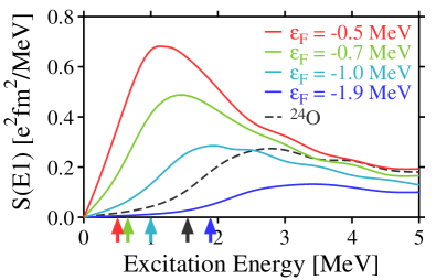
Figure 3: (Color online) Neutron Fermi level dependence of low-lying $E1$ strength. The solid lines from upper to lower correspond to the calculations with the neutron Fermi level $\varepsilon_{F}=-0.5$, $-0.7$, $-1.0$, and $-1.9$ MeV, respectively. The dashed line is the result of ²⁴O with $f_{0}=0.884$ corresponding to $\varepsilon_{F}=0.5$ MeV in ²²C. The SIII interaction is used with modification.

Next we discuss the low-lying $E1$ strength obtained by the self-consistent RPA calculation. Figure 3 demonstrates how the low-lying $E1$ strength develops as the neutron Fermi level $\varepsilon_{F}$ gets closer to zero energy. We calculate the low-lying $E1$ strength with the original SIII interaction ($\varepsilon_{F}=-1.9$ MeV), together with the modified interactions that give $\varepsilon_{F}=-1.0$ MeV, $\varepsilon_{F}=-0.70$ MeV (corresponding to adjusting the rms matter radius to 3.7 fm Horiuchi06 ), and $\varepsilon_{F}=-0.50$ MeV. The arrows denote the absolute value of $\varepsilon_{F}$, indicating the threshold of excitation to the continuum states. The $E1$ strength rises up not from the threshold but from zero excitation energy because we calculate the response function at a complex energy with 0.50 MeV of imaginary part. In the case of the original SIII interaction, no prominent $E1$ strength is found. As the Fermi energy $\varepsilon_{F}$ approaches zero energy, the low-lying $E1$ strength develops, especially at $\varepsilon_{F}\mathop{\vbox{ \offinterlineskip\hbox{$>$}\hbox to7.7778pt{\hss\hbox{$\sim$}\hss}}}-1.0$ MeV. This trend is known through the result of the three-body cluster model assuming an inert core Ershov12 . When $\varepsilon_{F}=-0.50$ MeV, summed $E1$ strengths up to 3.0, 4.0 and 5.0 MeV are 1.38, 1,65, and 1.85 $e^{2}$fm², respectively, which is comparable to the strength of ¹¹Li Nakamura06 .

We apply the same factor $f_{0}=0.884$ for ²⁴O, which corresponds to setting $\varepsilon_{F}=-0.5$ MeV in ²²C. Even though both ²²C and ²⁴O are neutron drip-line nuclei, additional two protons shrink the matter (neutron) radius, 3.89 fm $\to$ 3.42 fm (4.23 fm $\to$ 3.64 fm), and shift down the neutron Fermi level by 1 MeV. Consequently, the low-lying $E1$ strength of ²⁴O is not prominent, as shown in Fig. 3.

III.5 Comparison with giant dipole resonance

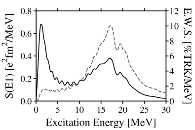
Figure 4: $E1$ strength distribution (solid line, left axis) and energy-weighted sum value (grayed dashed line, right axis) of ²²C obtained by setting $\varepsilon_{F}=-0.50$ MeV with SIII interaction.

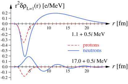
Figure 5: (Color online) Dipole transition densities at the peaks of low-lying $E1$ mode (1.1 MeV) and GDR (17.0 MeV).

An interesting property in drip-line nuclei is the large low-lying $E1$ strength comparable with that of the giant dipole resonance (GDR). The full $E1$ strength distribution with $\varepsilon_{F}=-0.5$ MeV is shown in Fig. 4. Some oscillations appearing at around the excitation energy $\omega\sim 5-10$ MeV come from the discretized continuum state and others from proton single particle-hole excitations from bound to bound states such as $1p_{3/2}\to 1d_{5/2}$. The peak height of the low-lying $E1$ strength in the present calculation is higher than that of the GDR. This is very unusual. The peak height of the observed low-lying $E1$ strength (PDR) in heavy neutron-rich nuclei such as ¹³²Sn Adrich05 is always lower than half of the height of the GDR. In fact, the calculated low-lying $E1$ strength carries about 1/3 of the total $E1$ strength. Though the peak height depends on the smearing width $\gamma$, we confirm that the peak of low-lying $E1$ strength is higher than the GDR when $\gamma\mathop{\vbox{ \offinterlineskip\hbox{$<$}\hbox to7.7778pt{\hss\hbox{$\sim$}\hss}}}3$ MeV. Our calculation demonstrates that the “pygmy” dipole resonance could be a “giant” low-lying dipole resonance in neutron drip-line nuclei. The energy-weighted sum of $E1$ strength is also plotted in Fig. 4, but its discussion will be given later in Sec. III.6.

In Fig. 5, we plot the dipole transition densities

$$r^{2}\delta\rho_{L=1}(r)=r^{2}\int d\Omega\,\,Y_{1}(\Omega)\delta\rho(\mbox{\boldmath$r$})$$ (9)

of protons and neutrons at the peaks of the low-lying $E1$ (1.1 MeV) and the GDR (17.0 MeV). The GDR transition densities display out-of-phase densities between protons and neutrons, which is typical for the GDR. Because of the halo structure in the ground state, the neutron transition density of the GDR has an oscillating extended tail. For the low-lying $E1$ case, the transition densities look like the oscillation of the outer neutron against the inner core, namely, the protons and neutrons inside the core nucleus oscillates in phase and only those neutrons residing far outside the core move out of phase against the inner core, similar to the classical picture of PDR Suzuki90 . Due to the loosely bound Fermi level with $\varepsilon_{F}=-0.50$ MeV, the neutron transition density has a quite long tail spreading to $r\sim 25$ fm, which indicates excitations from $2s_{1/2}$ orbit to the low-energy continuum states.

III.6 Cluster sum rule value

The sum rule is useful for a qualitative estimation of the contribution of the low-lying $E1$ strength. The energy-weighted sum rule is given by

$$S_{\mathrm{TRK}}=\frac{9e^{2}}{4\pi}\frac{\hbar^{2}}{2m}\frac{NZ}{A}.$$ (10)

This is known as the classical Thomas-Reiche-Kuhn (TRK) sum rule. The calculated low-lying $E1$ strength carries a sizable contribution despite the quite small excitation energy. As shown in Fig. 4, the low-lying $E1$ strength distribution exhausts 6.2, 11.0 and 15.4 % of the TRK sum rule when the strength is accumulated up to the excitation energy 5, 8 and 10 MeV, respectively. This is comparable to ⁶He Aumann99 and ¹¹Li Zinser97 , and is larger than those of the observed PDRs in heavier nuclei.

The low-lying $E1$ strength in light nuclei such as He and Be isotopes is often analyzed with use of the cluster model. Suppose that ²²C has a cluster-like structure, i.e., two neutrons coupled to the ²⁰C core. Then the energy-weighted cluster sum rule is evaluated as Alhassid82 ; Sagawa90

$$S_{\mathrm{clus}}=\frac{9e^{2}}{4\pi}\frac{\hbar^{2}}{2m}\frac{2Z^{2}}{A\left(A-2\right)}.$$ (11)

The cumulative energy-weighted sum value, $S(E_{c})=\int^{E_{c}}E^{\prime}S(E^{\prime};E1)dE^{\prime}$, exceeds $S_{\mathrm{clus}}$ at $E_{c}=3.3$ MeV in the case of $\varepsilon_{F}=-0.50$ MeV. Even for $\varepsilon_{F}=-0.70$ MeV or $-1.0$ MeV, it exceeds $S_{\mathrm{clus}}$ at $E_{c}=3.9$ MeV and 5.0 MeV, respectively. This means that the three-body model with the ²⁰C core and two neutrons is not supported in the present approach at least for $\varepsilon_{F}\mathop{\vbox{ \offinterlineskip\hbox{$>$}\hbox to7.7778pt{\hss\hbox{$\sim$}\hss}}}-1.0$ MeV. Exceeding the cluster sum rule indicates some other contributions coming from a core excitation, such as excitations from $1d_{5/2}$ orbit. Due to the core excitation, the non-energy-weighted cluster sum rule in fact does not work for the investigation of the calculated low-lying $E1$ strength. In the following, we show that a simple picture of the PDR, two valence neutrons oscillating against the ²⁰C core, is not fully supported by the present calculation. Contributions of the core excitation are present and discussed in the Sec. III.7

III.7 Core excitation: Role of $d_{5/2}$ state

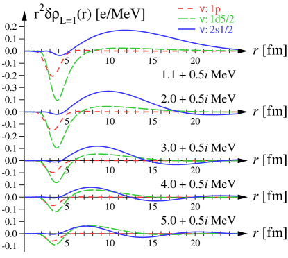
Figure 6: (Color online) Neutron transition densities decomposed to the occupied orbits, $1p$ (red), $1d_{5/2}$ (green), and $2s_{1/2}$ (blue) orbits, as a function of radius. Omitted transition density from $1s_{1/2}$ orbit is negligible.

As is mentioned above, the neutron excitations from $1d_{5/2}$ orbit may contribute to the low-lying $E1$ strength. Moreover, the calculated low-lying $E1$ strength has a large tail at excitation energy $\omega\mathop{\vbox{ \offinterlineskip\hbox{$>$}\hbox to7.7778pt{\hss\hbox{$\sim$}\hss}}}$ 2 MeV (See Fig. 3), in contrast to those of the three-body calculation Ershov12 . This difference supports some contributions of $1d_{5/2}$ orbit. Figure 6 demonstrates that the excitations from $1d_{5/2}$ orbit play a role of enhancing the $E1$ strength. We plot the neutron transition densities at a peak of the $E1$ strength, 1.1 MeV, and excitation energies from 2.0 MeV to 5.0 MeV with a spacing of 1.0 MeV. The transition densities are decomposed to the occupied orbits, namely, the decomposed ones are calculated by Eqs. (3) and (9) but the index $i$ runs over only the corresponding orbits and the sum of them is equal to the transition density in Fig. 5. At the peak position, the decomposed transition densities are divided to that of $2s_{1/2}$ orbit and the others. The transition density of $2s_{1/2}$ orbit has a long tail up to $r\sim 25$ fm, describing excitations to the low-energy continuum state. The other transition densities (including proton transition densities) have the sign opposite to the $2s_{1/2}$ transition density and their contributions are small at $r\mathop{\vbox{ \offinterlineskip\hbox{$>$}\hbox to7.7778pt{\hss\hbox{$\sim$}\hss}}}5$ fm, suggesting a recoil of the ²⁰C core. Therefore, the transition densities at 1.1 MeV show that two neutrons are excited to continuum state and go away from the remaining core. Our RPA calculation produces results similar to the three-body cluster model at the peak position Ershov12 . Nevertheless, it is seen even in 1.1 MeV state that a part of neutrons in $1d_{5/2}$ orbit is also excited to the continuum state. As excitation energy increases, the $2s_{1/2}$ transition density gradually becomes small, whereas the contribution of $1d_{5/2}\to$ continuum states develops and eventually become comparable to that of $2s_{1/2}$ orbit at 5.0 MeV excitation energy. This $1d_{5/2}$ contribution lifts the $E1$ strength at $E\mathop{\vbox{ \offinterlineskip\hbox{$>$}\hbox to7.7778pt{\hss\hbox{$\sim$}\hss}}}$ 2 MeV and produces the long tail of the low-lying $E1$ strength.

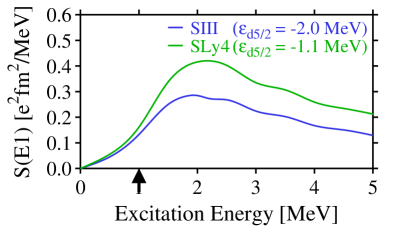
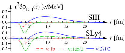
Figure 7: (Color online) Comparison of low-lying $E1$ strength (upper) and transition densities (lower) at peak position calculated with SIII and SLy4 interactions that are modified to set $\varepsilon_{F}=-1.0$ MeV.

Comparison of low-lying $E1$ strengths calculated with the same $\varepsilon_{F}$ but different interactions shows more clearly the role of the $1d_{5/2}$ orbit because the low-lying $E1$ strength distribution in neutron drip-line nuclei is not sensitive to the interaction itself used in calculation, but sensitive to the single-particle properties near the Fermi level. The upper panel of Fig. 7 shows the low-lying $E1$ strength obtained by setting $\varepsilon_{F}=-1.0$ MeV with the SIII and SLy4 interactions. The SLy4 (SIII) interaction with $\varepsilon_{F}=-1.0$ MeV yields $\varepsilon_{d5/2}=-1.1$ MeV ($-2.0$ MeV). While the peak position of the low-lying $E1$ strength is almost the same due to the same $\varepsilon_{F}$, the $E1$ strength with SLy4 is larger than that with SIII. This originates from the $1d_{5/2}$ orbit, as shown in the lower panel of Fig. 7 which compares the decomposed transition densities at the peak positions. The $2s_{1/2}$ transition densities are quite similar to each other but clear difference is seen in the $1d_{5/2}$ transition densities at $r\sim 7-20$ fm. Such difference, though it is apparently small, enhances the $E1$ strength by a factor $\sim 1.5$. This indicates the importance of the core excitation or explicit treatment of the $1d_{5/2}$ orbit in ²²C.

III.8 Validity of calculation

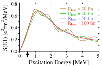
Figure 8: (Color online) Box size dependence of the calculated $E1$ strength with $\varepsilon_{F}=-0.50$ MeV.

Here we comment on the validity and accuracy of our calculation for the low-lying $E1$ excitation in drip-line nuclei. Since the loosely bound $2s_{1/2}$ orbit with $\varepsilon_{s1/2}=-0.50$ MeV is spatially quite spread and couples with the continuum state by a small excitation energy, a large calculation space is needed to describe the low-lying $E1$ strength properly. Figure 8 shows the box size dependence of the calculated low-lying $E1$ strength with $\gamma=1$ MeV for $R_{\mathrm{box}}=$ 30, 40, 50, and 100 fm. The summed $E1$ strength below 5 MeV is not sensitive to $R_{\mathrm{box}}$; 1.855, 1.809, 1.851, and 1.849 $e^{2}\mathrm{fm}^{2}$ for $R_{\mathrm{box}}=$ 30, 40, 50, and 100 fm, respectively. While the $E1$ strength distributions with $R_{\mathrm{box}}=$ 30 and 40 fm have oscillations stemming from discretized continuum states, the result with $R_{\mathrm{box}}=$ 50 fm shows practically no oscillation and agrees well with $R_{\mathrm{box}}=$ 100 fm. Difference between the calculated $E1$ strengths with $R_{\mathrm{box}}=$ 50 and 100 fm is less than 0.5 % except for very low-energy region, $\omega\mathop{\vbox{ \offinterlineskip\hbox{$<$}\hbox to7.7778pt{\hss\hbox{$\sim$}\hss}}}0.5$ MeV. Thus, the box size $R_{\mathrm{box}}=$ 50 fm we employ in this paper is large enough for quantitative study of the low-lying $E1$ mode with $\gamma=1$ MeV.

Next, let us check the validity of the RPA and the mixture of the spurious state. It is known that the RPA becomes unreliable for low-lying states with very high collectivity, because the RPA assumes the small amplitude nature. This can be examined by investigating the magnitude of forward and backward amplitudes. The RPA breaks down if the backward amplitudes become comparable to the forward ones. For this purpose, we perform the RPA calculation with the diagonalization method by using a revised version of the RPA code in Ref. Inakura06 with the same dipole operator (4) and for box size of $R_{\mathrm{box}}=40$ fm. The spurious state appears at excitation energy 0.15 MeV. For this state, the squared modulus of the backward amplitude, $\left|Y\right|^{2}\equiv\sum_{i}\int d\mbox{\boldmath$r$}\,\left|Y_{i}(\mbox{\boldmath$r$})\right|^{2}$, is 15.0. This means the forward amplitude, $|X|^{2}=16.0$. In contrast, the lowest-energy physical state appears at 0.75 MeV and its $\left|Y\right|^{2}$ is 0.042. Therefore, the present RPA calculation does not break down for the low-lying $E1$ modes.

We calculate isoscalar dipole strength (i.e., spurious component) and confirm that the spurious state is well separated from the physical states. The isoscalar dipole strength is calculated by Eq. (5) but for an isoscalar dipole operator $D_{\mathrm{IS}}=e\sum_{i=1}^{A}r_{i}Y_{1}(\Omega)$. The isoscalar dipole strength for the low-lying peak is satisfactorily small, $\left|\langle n|D_{\mathrm{IS}}|0\rangle\right|^{2}<2\times 10^{-3}$ e²fm², which is about 1 % of the corresponding $E1$ strength. Therefore, numerical calculation of the spurious state is not serious in the present calculation.

It is worthy to note that the low-lying $E1$ strengths smeared by Lorentzians (6) with $\gamma=1$ MeV is underestimated compared with those calculated by the diagonalization method which corresponds to a limit of $\gamma\to 0$ MeV. For example, summations of the $E1$ strengths below 5 MeV, calculated by the diagonalization method and the response function with $\gamma=1$ MeV, are 2.366 and 1.809 $e^{2}\mathrm{fm}^{2}$, respectively, for $R_{\mathrm{box}}=$ 40 fm. Such underestimation is noticeable for low-lying $E1$ strengths but not for the GDR region. Small $\gamma$ is obviously better but requires large calculation space for obtaining converged $E1$ strength distribution. Thus we employ the $\gamma=1$ MeV in this paper. In addition, we do not take into account the pairing correlation in the present calculations. The pairing correlation does not change the qualitative nature of the $E1$ strength distribution Ebata10 ; Ebata11 , but, may enhance the low-energy $E1$ strength. Therefore, the calculated low-lying $E1$ strength may become even larger in more realistic calculations.

IV Conclusions

We have studied the ground state properties and the low-lying $E1$ strength of ²²C using the mean-field approach which does not assume the ²⁰C core. Since the original Skyrme interactions we chose do not give a consistent description of the observed ground state properties such as the nuclear size, we adjusted the central part of the Skyrme potential. When we set the neutron Fermi level $\varepsilon_{F}\mathop{\vbox{ \offinterlineskip\hbox{$>$}\hbox to7.7778pt{\hss\hbox{$\sim$}\hss}}}-1.0$ MeV, the obtained total reaction cross section reasonably agrees with the measured value. With $\varepsilon_{F}\mathop{\vbox{ \offinterlineskip\hbox{$>$}\hbox to7.7778pt{\hss\hbox{$\sim$}\hss}}}-0.5$ MeV, the calculation predicts the low-lying $E1$ strength comparable with that of the giant dipole resonance. The energy weighted cluster sum rule assuming a ²⁰C core is tested. The cumulative $E1$ strength exceeds the sum rule at very low energy due to the contribution of the “core” excitation. Such large low-lying $E1$ strength consists mainly of the excitations from $2s_{1/2}$ and $1d_{5/2}$ orbits to the continuum states. As the excitation energy increases, the contribution of $1d_{5/2}$ orbit to the low-lying $E1$ strength develops and could become comparable to that of $2s_{1/2}$ orbit. A precise measurement of the low-lying $E1$ strength and a careful analysis of the neutron orbits, e.g., the momentum distribution of ²⁰C fragment of ²²C breakup Kobayashi12 , are desired to clarify the role of the core excitation in ²²C.

References

- (1) W. Horiuchi and Y. Suzuki, Phys. Rev. C 74, 034311 (2006).
- (2) K. Tanaka et al., Phys. Rev. Lett. 104, 062701 (2010).
- (3) L. Gaudefroy et al., Phys. Rev. Lett. 109, 202503 (2012).
- (4) M.T. Yamashita, R.S. Marques de Carvalho, T. Frederico, Lauro Tomio, Phys. Lett. B 697 (2011) 90-93.
- (5) H.T. Fortune and R. Sherr, Phys. Rev. C 85, 027303 (2012).
- (6) S.N. Ershov, J.S. Vaagen, M.V. Zhukov, Phys. Rev. C 86, 034331 (2012).
- (7) A. Carbone et al., Phys. Rev. C 81, 041301(R) (2010), and references therein.
- (8) T. Otsuka, Y. Utsuno, R. Fujimoto, B.A. Brown, M. Honma, and T. Mizusaki, Eur. Phys. J. A 15, 151-155 (2002).
- (9) I. Hamamoto, Phys. Rev. C 76, 054319 (2007).
- (10) D. Vautherin and D.M. Brink, Phys. Rev. C 5, 626 (1972).
- (11) T. Nakatsukasa and K. Yabana, Phys. Rev. C 71, 024301 (2005).
- (12) H. Flocard, S.E. Koonin, and M.S. Weiss, Phys. Rev. C 17, 1682 (1978).
- (13) K.T.R. Davies, H. Flocard, S. Krieger, and M.S. Weiss, Nucl. Phys. A 342, 111 (1980).
- (14) P. Ring and P. Schuck, The Nuclear Many-Body Problem, (Springer-Verlag, 1980).
- (15) S.C. Eisenstat, H.C. Elman, and M.H. Schultz, SIAM J. Numer, Anal, 20, 345-357 (1983).
- (16) T. Nakatsukasa, T. Inakura, and K. Yabana, Phys. Rev. C 76, 024318 (2007).
- (17) T. Inakura, T. Nakatsukasa, and K. Yabana, Phys. Rev. C 80, 044301 (2009).
- (18) T. Inakura, T. Nakatsukasa, and K. Yabana, Phys. Rev. C 84, 021302(R) (2011).
- (19) P. Avogadro and T. Nakatsukasa, Phys. Rev. C 84, 014314 (2011).
- (20) M. Stoitsov, M. Kortelainen, T. Nakatsukasa, C. Losa, and W. Nazarewicz, Phys. Rev. C 84, 041305(R) (2011).
- (21) P. Avogadro and T. Nakatsukasa, Phys. Rev. C 87, 014331 (2013).
- (22) H. Z. Liang, T. Nakatsukasa, Z. Niu, and J. Meng, Phys. Rev. C 87, 054310 (2013).
- (23) N. Hinohara, M. Kortelainen, and W. Nazarewicz, Phys. Rev. C 87, 064309 (2013).
- (24) M. Beiner, H. Flocard, Nguyen van Giai, and P. Quentin, Nucl. Phys. A 238, 29 (1975).
- (25) E. Chabanat, P. Bonche, P. Haensel, J. Mayer, and R. Schaeffer, Nucl. Phys. A 627, 231 (1998).
- (26) Nguyen Van Giai, and H. Sagawa, Phys. Lett. B 106, 379 (1981).
- (27) J. Bartel, P. Quentin, M. Brack, C. Guet, and H.B. Håkansson, Nucl. Phys. A 386, 79 (1982).
- (28) P. Klüpfel, P.-G. Reinhard, T.J. Bürvenich, and J.A. Maruhn, Phys. Rev. C 79, 034310 (2009)
- (29) M. Kortelainen, J. McDonnell, W. Nazarewicz, P.-G. Reinhard, J. Sarich, N. Schunck, M.V. Stoitsov, and S.M. Wild, Phys. Rev. C 85, 024304 (2012)
- (30) P.-G. Reinhard and H. Flocard, Nucl. Phys. A 584, 467 (1995).
- (31) K. Bennaceur and J. Dobaczewski, Computer Physics Communications 168 (2005) 96-122.
- (32) M.V. Stoitsov, N. Schunck, M. Kortelainen, N. Michel, H. Nam, E. Olsen, J. Sarich, and S. Wild, Computer Physics Communications 184 (2013) 1592-1604.
- (33) R. J. Glauber, in Lecture in Theoretical Physics, edited by W. E. Brittin and L. G. Dunham, Vol. 1 (Interscience, New York, 1959), p. 315.
- (34) B. Abu-Ibrahim, W. Horiuchi, A. Kohama, and Y. Suzuki, Phys. Rev. C 77, 034607 (2008).
- (35) W. Horiuchi, Y. Suzuki, B. Abu-Ibrahim, and A. Kohama, Phys. Phys. C 75, 044607 (2007).
- (36) B. Abu-Ibrahim and Y. Suzuki, Phys. Rev. C 61, 051601(R) (2000).
- (37) B. Abu-Ibrahim, S. Iwasaki, W. Horiuchi, A. Kohama, and Y. Suzuki, J. Phys. Soc. Jpn. 78, 044201 (2009).
- (38) W. Horiuchi, T. Inakura, T. Nakatsukasa, and Y. Suzuki, Phys. Rev. C 86, 024614 (2012).
- (39) T. Nakamura et al., Phys. Rrv. Lett. 96, 252502 (2006)
- (40) P. Adrich et al., Phys. Rev. Lett. 95, 132501 (2005).
- (41) Y. Suzuki, K. Ikeda, and H. Sato, Prog. Theor. Phys. 83, 180 (1990).
- (42) T. Aumann et al., Phys. Rev. C 59, 1252-1262 (1999).
- (43) M. Zinser et al., Nucl. Phys. A 619, 151 (1997).
- (44) Y. Alhassid, M. Gai, and G.F. Bertsch, Phys. Rev. Lett. 49, 1482 (1982).
- (45) H. Sagawa and M. Honma, Phys. Lett. B 251, 17 (1990).
- (46) T. Inakura, H. Imagawa, Y. Hashimoto, S. Mizutori, M. Yamagami K. Matsuyanagi, Nucl. Phys. A 768, 61 (2006).
- (47) S. Ebata, T. Nakatsukasa, T. Inakura, K. Yoshida, Y. Hashimoto, and K. Yabana, Phys. Rev. C 82, 034306 (2010).
- (48) S. Ebata, T. Nakatsukasa, and T. Inakura, AIP conf. Proc. 1484, 427 (2012); J. Phys. Conf. Ser. 381, 012104 (2012).
- (49) N. Kobayashi et al., Phys. Rev. C 86, 054604 (2012).