Asymptotic Error Performance Analysis of Spatial Modulation under Generalized Fading

Abstract

This letter presents a comprehensive framework analyzing the asymptotic error performance of a multiple-input-multiple-output (MIMO) wireless system employing spatial modulation (SM) with maximum likelihood detection and perfect channel state information. Generic analytical expressions for the diversity and coding gains are deduced that reveal fundamental properties of MIMO SM systems. The presented analysis can be used to obtain closed-form upper bounds for the average bit error probability (ABEP) of MIMO SM systems under generalized fading which become asymptotically tight in the high signal-to-noise ratio (SNR) region.

I Introduction

Spatial modulation (SM) is an efficient, low-complexity transmission technique for multiple-input-multiple-output (MIMO) wireless systems which achieves a spatial multiplexing gain, at the same time avoiding inter-channel interference without requiring synchronization between the transmit antennas [1, 2]. A fundamental concept in SM is the three-dimensional constellation diagram [2] where each spatial constellation point, corresponding to the transmit antenna index, defines an independent complex plane of signal constellation points. When the information carrying entity is solely the transmit-antenna index, SM is reduced to the space shift keying (SSK) modulation, where a single transmit-antenna is activated each time to transmit a symbol.

Several analytical frameworks assessing the error performance of SM systems over fading channels are available in the technical literature. For example, [3] and [4] employ a moment generating function (MGF) based approach to evaluate the average bit error probability (ABEP) of SSK in the presence of Nakagami-$m$ and Rice fading. The MGF-based approach presented in these works is extended to the most general case of SM in [5], where tight error performance bounds are deduced. In a recent work [6], a generic approach for the performance of SSK was proposed, assuming generalized fading envelopes and uniformly distributed channel phases.

The above cited frameworks provide an exact performance analysis of SM systems over the entire signal-to-noise ratio (SNR) region; however, single integrals with finite or infinite limits have to be readily evaluated via numerical integration to this end. Moreover, these frameworks do not provide enough insight into the parameters affecting system performance in terms of diversity and coding gains. In an attempt to bridge this gap, closed-form expressions for the asymptotic performance of SM systems are provided in [5] and [7].

Motivated by the above cited works, the objective of the current letter is twofold: a) To deduce closed-form upper bounds for the ABEP of SM MIMO systems operating over generalized fading environments which become asymptotically tight in the high SNR region, and b) to provide important considerations about the diversity and coding gains of SM in the presence of generalized fading. The proposed analysis is tested and verified by numerically evaluated results accompanied with Monte Carlo simulations as well as by reducing them to several special cases available in the literature.

II Mathematical Tools

In this section, new mathematical tools are presented that simplify the performance evaluation of SM systems. According to [5], the evaluation of the ABEP of SM requires the solution of integrals of the form

$$\mathcal{I}(A,L)=\frac{1}{\pi}\int_{0}^{\pi/2}\prod_{\ell=1}^{L}\left[\mathcal{M}_{Z_{\ell}}\left(\frac{A}{2\sin^{2}\theta}\right)\right]\mathrm{d}\theta,\,A>0$$ (1)

where $\mathcal{M}_{Z_{\ell}}(\cdot)$ denotes the MGF of the random variable $Z_{\ell}$ defined as $Z_{\ell}=|z_{2,\ell}-z_{1,\ell}|^{2}$ with $z_{i,\ell}=\alpha_{i,\ell}\exp(\jmath\Phi_{2,\ell})$ being random vectors having arbitrarily distributed magnitudes $\alpha_{i,\ell}$ and phases $\Phi_{i,\ell}$, $\forall i\in\{1,2\}$. In general, closed form expressions for $\mathcal{I}(A,L)$ are very difficult to be obtained and numerical integration is used instead (see for example [3], [4] and [6]). In [7], by exploiting asymptotic analysis, closed-form approximations for $\mathcal{I}(A,L)$ are provided for high values of $A$, assuming that $\alpha_{i,\ell}$ are Nakagami-$m$ distributed random variables and $\Phi_{i,\ell}$ uniformly distributed in $[0,2\pi]$.

In the following analysis, a generic solution of (1) for high values of $A$ will be deduced, assuming that $\alpha_{i,\ell}$ are arbitrarily distributed random variables and $\Phi_{i,\ell}$ are uniformly distributed in $[0,2\pi]$. In order to obtain such an expression, [8, Proposition 3] is employed to approximate $\mathcal{M}_{Z_{\ell}}(s)$ for $s\rightarrow\infty$ as

$$|\mathcal{M}_{Z_{\ell}}(s)|=c_{\ell}|s|^{-d_{\ell}}+o(|s|^{-d_{\ell}}),\,s\rightarrow\infty$$ (2)

The MGF of $Z_{\ell}$ is given by [6, Eq. (9)] as

$$\mathcal{M}_{Z_{\ell}}(s)=\frac{1}{2s}\int_{0}^{\infty}R\mathrm{e}^{-\frac{R^{2}}{4s}}\left[\prod_{i=1}^{2}\mathcal{H}_{0,R}\left\{\frac{f_{\alpha_{i,\ell}}(r)}{r}\right\}\right]\mathrm{d}R$$ (3)

where $f_{a_{i,\ell}}(r)$ is the probability density function of $\alpha_{i,\ell}$ and $\mathcal{H}_{0,R}\{\cdot\}$ denotes the zeroth order Hankel transform [9, Eq. (9.11)]. Since $\mathrm{e}^{-\frac{R^{2}}{4s}}=o(\frac{1}{s})$ as $s\rightarrow\infty$, the approximation $\mathrm{e}^{-\frac{R^{2}}{4s}}/2s\overset{s\rightarrow\infty}{\approx}1/2s$ can be employed in (3) to yield

$$\mathcal{M}_{Z_{\ell}}(s)\overset{s\rightarrow\infty}{\approx}\frac{1}{2s}\int_{0}^{\infty}R\left[\prod_{i=1}^{2}\mathcal{H}_{0,R}\left\{\frac{f_{\alpha_{{i},\ell}}(r)}{r}\right\}\right]\mathrm{d}R$$ (4)

Changing the information variable $R^{2}$ to $y$ and comparing (4) with (2), it is readily deduced that $d_{\ell}=1$ and

$$c_{\ell}=\frac{1}{4}\int_{0}^{\infty}\prod_{i=1}^{2}\mathcal{H}_{0,\sqrt{y}}\left\{\frac{f_{\alpha_{i,\ell}}(r)}{r}\right\}\mathrm{d}y$$ (5)

Finally, by substituting (2) and (5) into (1), it is deduced that for high values of $A$, $\mathcal{I}(A,L)$ can be approximated by

$$\mathcal{I}(A,L)\overset{A\gg 1}{\approx}\frac{2^{L-1}\Gamma\left(L+\frac{1}{2}\right)}{\sqrt{\pi}\Gamma\left(L+1\right)}\left[\prod_{\ell=1}^{L}c_{\ell}\right]A^{-L}$$ (6)

where $\Gamma(\cdot)$ is the gamma function [10, Eq. (8.310/1)].

$$\begin{split}&c_{\ell}=\frac{b_{s,1,\ell}b_{1,\ell}}{\Gamma(m_{1,\ell})\Gamma(m_{2,\ell})\Gamma(m_{s,1,\ell})\Gamma(m_{s,2,\ell})\Omega_{1,\ell}}H\begin{subarray}{c}2,2\\ 2,2\end{subarray}\left[\frac{\Omega_{2,\ell}b_{1,\ell}b_{s,1,\ell}}{\Omega_{1,\ell}b_{2,\ell}b_{s,2,\ell}}\left|\begin{subarray}{c}\left(1-m_{2,\ell},\frac{2}{\beta_{2,\ell}}\right),\left(1-m_{s,2,\ell},\frac{2}{\beta_{s,2,\ell}}\right)\\ \hbox{}\\ \left(m_{1,\ell}-\frac{2}{\beta_{1,\ell}},\frac{2}{\beta_{1,\ell}}\right),\left(m_{s,1,\ell}-\frac{2}{\beta_{s,1,\ell}},\frac{2}{\beta_{s,1,\ell}}\right)\end{subarray}\right.\right]\end{split}$$ (9)

$$\begin{split}&c_{\ell}=\frac{\Gamma(-1+m_{2,\ell}+m_{s,1,\ell})\Gamma(-1+m_{s,2,\ell}+m_{s,1,\ell})\Gamma(-1+m_{2,\ell}+m_{1,\ell})\Gamma(-1+m_{s,2,\ell}+m_{1,\ell})}{\Gamma\left(-2+\sum_{i=1}^{2}\left[m_{i,\ell}+m_{s,i,\ell}\right]\right)\left[\prod_{i=1}^{2}\Gamma(m_{i,\ell})\Gamma(m_{s,i,\ell})\right]\left(\frac{m_{s,1,\ell}m_{1,\ell}}{\Omega_{1,\ell}}\right)^{m_{2,\ell}-1}}\\ &\times\left(\frac{m_{2,\ell}m_{s,2,\ell}}{\Omega_{2,\ell}}\right)^{m_{2,\ell}}{}_{2}F_{1}\left(-1+\sum_{i=1}^{2}m_{i,\ell},-1+m_{2,\ell}+m_{s,1,\ell};-2+\sum_{i=1}^{2}\left[m_{i,\ell}+m_{s,i,\ell}\right],1-\frac{\Omega_{1,\ell}m_{2,\ell}m_{s,2,\ell}}{\Omega_{2,\ell}m_{1,\ell}m_{s,1,\ell}}\right)\end{split}$$ (11)

It is noted that $c_{\ell}$ and henceforth $\mathcal{I}(A,L)$ can be easily obtained in closed-form by employing Mellin transform techniques, provided that a closed-form expression for $\mathcal{H}_{0,\sqrt{y}}\left\{\frac{f_{\alpha_{i,\ell}}(r)}{r}\right\}$ is readily available. In what follows, a closed form expression for $c_{\ell}$ will be deduced assuming that $\alpha_{i,\ell}$ follow the Extended Generalized-$\mathcal{K}$ (EGK) distribution. The motivation behind the choice of this specific model is that the EGK distribution exhibits good tail properties and encompasses most of the well-known fading distributions either as special or as limiting cases [11, Table I]. Simplified expressions for the special cases of Generalized-$\mathcal{K}$ and the Nakagami-$m$ distributions are also deduced.

II-A The Extended Generalized-$\mathcal{K}$ case

Under EGK fading, the zeroth order Hankel transform of $f_{\alpha_{i,\ell}}(r)/r$ is determined in closed-form as [6, Eq. (11)]

$$\begin{split}\mathcal{H}_{0,R}\left\{\frac{f_{\alpha_{i,\ell}}(r)}{r}\right\}&=\frac{H\begin{subarray}{c}2,1\\ 2,2\end{subarray}\left[\frac{4b_{s,i,\ell}\,{b}_{i,\ell}}{R^{2}\Omega_{i,\ell}}\left|\begin{subarray}{c}(1,1),\ (1,1)\\ \hbox{}\\ \Xi_{\ell}\end{subarray}\right.\right]}{\Gamma(m_{i,\ell})\Gamma(m_{s,i,\ell})}\end{split}$$ (7)

where $H\,\begin{subarray}{c}m,n\\ p,q\end{subarray}[\cdot]$ is the Fox’s H-function [12, Eq. (8.3.1)], $\Xi_{\ell}\triangleq\left\{\left(m_{i,\ell},\frac{2}{\beta_{i,\ell}}\right),\left(m_{s,i,\ell},\frac{2}{\beta_{s,i,\ell}}\right)\right\}$. In (7), $m_{i,\ell}$ $(0.5<m_{i,\ell}<\infty)$ and $\beta_{i,\ell}$ $(0<\beta_{i,\ell}<\infty)$ represent the fading severity and the fading shaping factor, respectively, $m_{s,i,\ell}$ $(0.5<m_{s,i,\ell}<\infty)$ and $\beta_{s,i,\ell}$ $(0<\beta_{s,i,\ell}<\infty)$ represent the shadowing severity and the shadowing shaping factor, respectively, and $\Omega_{i,\ell}=\mathbb{E}\langle a_{i,\ell}^{2}\rangle$ with $\mathbb{E}\langle\cdot\rangle$ denoting expectation. Moreover, ${b}_{i,\ell}={\Gamma\left(m_{i,\ell}+\frac{2}{\beta_{i,\ell}}\right)}/{\Gamma(m_{i,\ell})}$ and $b_{s,i,\ell}={\Gamma\left(m_{s,i,\ell}+\frac{2}{\beta_{s,i,\ell}}\right)}/{\Gamma(m_{s,i,\ell})}$. By substituting (7) into (5) and employing [12, Eq. (2.25.1.1)] along with [12, Eq. (8.3.2.7)], $c_{\ell}$ can be evaluated from

$$c_{\ell}=A_{\ell}H\begin{subarray}{c}3,3\\ 4,4\end{subarray}\left[x_{\ell}\left|\begin{subarray}{c}(\Lambda_{1},\lambda_{1}),(\Lambda_{2},\lambda_{2}),(0,1),(0,1)\\ \hbox{}\\ (0,1),(M_{1},\mu_{1}),(M_{2},\mu_{2}),(0,1)\end{subarray}\right.\right]$$ (8)

where $A_{\ell}=\frac{b_{s,1,\ell}b_{1,\ell}}{\Gamma(m_{1,\ell})\Gamma(m_{2,\ell})\Gamma(m_{s,1,\ell})\Gamma(m_{s,2,\ell})\Omega_{1,\ell}}$, $x_{\ell}=\frac{\Omega_{2,\ell}b_{1,\ell}b_{s,1,\ell}}{\Omega_{1,\ell}b_{2,\ell}b_{s,2,\ell}}$, $\Lambda_{1}=1-m_{2,\ell}$, $\lambda_{1}={2}/{\beta_{2,\ell}}$, $\Lambda_{2}=1-m_{s,2,\ell}$, $\lambda_{2}={2}/{\beta_{s,2,\ell}}$, $M_{1}=m_{1,\ell}-{2}/{\beta_{1,\ell}}$, $\mu_{1}={2}/{\beta_{1,\ell}}$, $M_{2}=m_{s,1,\ell}-{2}/{\beta_{s,1,\ell}}$ and $\mu_{2}={2}/{\beta_{s,1,\ell}}$. The result in (8) can be reduced further by employing [12, Eq. (8.3.2.6)] yielding (9), on the top of the next page.

II-B The Generalized-$\mathcal{K}$ case

Under Generalized-$\mathcal{K}$ fading conditions, an expression for $c_{\ell}$ is readily obtained from (9) setting the fading shaping factor $\beta_{i,\ell}\rightarrow 2$ and the shadowing shaping factor $\beta_{s,i,\ell}\rightarrow 2$. Employing [12, Eq. (8.3.2.21)], (9) yields

$$\begin{split}&c_{\ell}=\mathcal{B}_{\ell}G\begin{subarray}{c}2,2\\ 2,2\end{subarray}\left[\frac{\Omega_{2,\ell}m_{1,\ell}m_{s,1,\ell}}{\Omega_{1,\ell}m_{2,\ell}m_{s,2,\ell}}\left|\begin{subarray}{c}1-m_{2,\ell},1-m_{s,2,\ell}\\ \hbox{}\\ m_{1,\ell}-1,m_{s,1,\ell}-1\end{subarray}\right.\right]\end{split}$$ (10)

where $G\,\begin{subarray}{c}m,n\\ p,q\end{subarray}[\cdot]$ is the Meijer’s G-function [10, Eq. (9.301)] and $\mathcal{B}_{\ell}=\frac{m_{s,1,\ell}m_{1,\ell}}{\Gamma(m_{1,\ell})\Gamma(m_{2,\ell})\Gamma(m_{s,1,\ell})\Gamma(m_{s,2,\ell})\Omega_{1,\ell}}$. Finally, employing the identity [15, Eq. (07.34.03.0871.01)], (10) can be further expressed in terms of the Gauss hypergeometric function ${}_{p}F_{q}(\cdot)$ [10, Eq. (9.14.1)] as (11), on the top of the next page.

II-C The Nakagami-$m$ case

For the special case of Nakagami-$m$ fading, an expression for $c_{\ell}$ is readily obtained from (10) setting the shadowing severity factor $m_{s,i,\ell}\rightarrow\infty$. Specifically, it can be shown that $c_{\ell}$ is reduced to a known result. Letting $m_{s,i,\ell}\rightarrow\infty$ in (10) and employing the definition of the Meijer’s G-function [12, Eq. (8.2.1.1)], $c_{\ell}$ can be written as

$$c_{\ell}=\frac{m_{1,\ell}(2\pi\jmath\Omega_{1,\ell})^{-1}}{\Gamma(m_{1,\ell})\Gamma(m_{2,\ell})}\int_{\mathcal{C}}\left(\frac{\Omega_{2,\ell}m_{1,\ell}}{\Omega_{1,\ell}m_{2,\ell}}\right)^{-u}\Gamma(m_{2,\ell}-u)$$

$$\times\Gamma(m_{1,\ell}-1+u)\left[\lim_{m_{s,1,\ell}\to\infty}\frac{m_{s,1,\ell}^{-u+1}\Gamma(m_{s,1,\ell}-1+u)}{\Gamma(m_{s,1,\ell})}\right]$$

$$\times\left[\lim_{m_{s,2,\ell}\to\infty}\frac{m_{s,2,\ell}^{u}\Gamma(m_{s,2,\ell}-u)}{\Gamma(m_{s,2,\ell})}\right]\mathrm{d}u$$ (12)

where $\mathcal{C}$ is the Mellin-Barnes contour. Employing the identity $\lim_{x\to\infty}\frac{x^{-u}\Gamma(x+u)}{\Gamma(x)}=1$ [10, Eq. (8.328)] along with [12, Eq. (8.2.1.1)], (II-C) is written as

$$\begin{split}&c_{\ell}=\frac{m_{1,\ell}}{\Gamma(m_{1,\ell})\Gamma(m_{2,\ell})\Omega_{1,\ell}}G\begin{subarray}{c}1,1\\ 1,1\end{subarray}\left[\frac{\Omega_{2,\ell}m_{1,\ell}}{\Omega_{1,\ell}m_{2,\ell}}\left|\begin{subarray}{c}1-m_{2,\ell}\\ \hbox{}\\ m_{1,\ell}-1\end{subarray}\right.\right]\end{split}$$ (13)

Finally, using the identity $G\begin{subarray}{c}1,1\\ 1,1\end{subarray}\left[x\left|\begin{subarray}{c}a\\ \hbox{}\\ b\end{subarray}\right.\right]=\Gamma(1-a+b)x^{b}(x+1)^{a-b-1}$ [15, 07.34.03.0271.01], $c_{\ell}$ is given from

$$\begin{split}c_{\ell}&=\left[\prod_{i=1}^{2}\frac{1}{\Gamma(m_{i,\ell})}\left(\frac{m_{i,\ell}}{\Omega_{i,\ell}}\right)^{m_{i,\ell}}\right]\Gamma\left(-1+\sum_{i=1}^{2}m_{i,\ell}\right)\\ &\times\left(\sum_{i=1}^{2}\frac{m_{i,\ell}}{\Omega_{i,\ell}}\right)^{1-\sum_{i=1}^{2}m_{i,\ell}}\end{split}$$ (14)

which is identical to [7, Eq. (4)].

III Application to the Performance analysis of Spatial Modulation

In this section, the results reported in Section II are applied to assess the asymptotic performance of SM systems.

III-A System Model

A $N_{t}\times N_{r}$ MIMO system employing SM is considered, equipped with $N_{t}$ transmit and $N_{r}$ receive antennas, which can send digital information via $M$ complex symbols, $\chi_{j}=|\chi_{j}|e^{\jmath\theta_{j}}$, $j=1,\ldots,M$. In the following and without loss of generality, two test cases are considered: i) A pure SSK system operating under independent and identically distributed (i.i.d) fading (Case I); and ii) A SM system operating under i.i.d fading with constant-modulus modulation i.e. $|\chi_{j}|=\kappa_{0}$, $\forall j=1,\ldots,M$ (Case II).

III-A1 Case I

Under the assumption of i.i.d fading, a tight upper bound for the ABEP of SSK can be obtained from [3, Eq. (35)], [7], as

$$\overline{P}\leq\frac{N_{t}}{2}{\rm PEP_{SSK}}(t_{1}\rightarrow t_{2})$$ (15)

where ${\rm PEP_{SSK}}(t_{1}\rightarrow t_{2})$ denotes the pairwise error probability related to the pair of transmit antennas $t_{1}$ and $t_{2}$, $t_{1},t_{2}=1,2,\ldots,N_{t}$, and it is the same for any pair $(t_{1},t_{2})$. The ${\rm PEP_{SSK}}(t_{1}\rightarrow t_{2})$ can be evaluated as [7, Eq. (1)]

$${\rm PEP_{SSK}}(t_{1}\rightarrow t_{2})=\frac{1}{\pi}\int_{0}^{\pi/2}\prod_{\ell=1}^{N_{r}}\left[\mathcal{M}_{\mathcal{Z}_{\ell}}\left(\frac{\overline{\gamma}}{2\sin^{2}\theta}\right)\right]\mathrm{d}\theta$$ (16)

where $\mathcal{Z}_{\ell}=|a_{t_{2},\ell}\exp(\jmath\phi_{t_{2},\ell})-a_{t_{1},\ell}\exp(\jmath\phi_{t_{1},\ell})|^{2}$, with $a_{t_{i},\ell}$ and $\phi_{t_{i},\ell}$ being the envelopes and phases of the link defined by the $t_{i}$-th transmit antenna and the $\ell$-th receive antenna. Moreover, $\overline{\gamma}=E_{s}/4N_{0}$ is the SNR where $E_{s}$ is the symbol energy and $N_{0}$ is the single-sided power spectral density of the additive white gaussian noise. For high values of $\overline{\gamma}$, it can be observed that ${\rm PEP_{SSK}}(t_{1}\rightarrow t_{2})$ can be readily evaluated employing (6) as ${\rm PEP_{SSK}}(t_{1}\rightarrow t_{2})\overset{\overline{\gamma}\gg 1}{\approx}\mathcal{I}\left(\overline{\gamma},N_{r}\right)$. Finally, from (6), it is evident that the diversity gain depends only on the number of the receive antennas and is independent of the fading severity. This finding is in agreement with relevant findings reported in [4] and [7]. The resulting coding gain can be obtained in closed-form from [8, Eq. (1)].

III-A2 Case II

The ABEP of SM can be tightly upper bounded as [5, Eq. (6)]

$$\overline{P} \leq\text{ABEP}_{\text{signal}}+\text{ABEP}_{\text{spatial}}+\text{ABEP}_{\text{joint}}$$ (17)

where $\text{ABEP}_{\text{signal}}$, $\text{ABEP}_{\text{spatial}}$ and $\text{ABEP}_{\text{joint}}$ show how the error performance of SM is affected by the signal constellation diagram, the spatial constellation diagram and the interaction of both signal and space constellation diagrams, respectively. Under generalized fading, the term $\text{ABEP}_{\text{signal}}$ when either $M$-ary phase shift keying ($M$-PSK) or $M$-ary quadrature amplitude modulation ($M$-QAM) are employed, can be readily evaluated using [5, Eqs. (7), (8)] and [5, Table I]. High-SNR asymptotically tight expressions for $\text{ABEP}_{\text{signal}}$ can also be obtained using [8]. Assuming constant modulus modulation $\text{ABEP}_{\text{spatial}}$ and $\text{ABEP}_{\text{joint}}$ can be obtained from [5, Eq. (10)] and [5, Eq. (11)], respectively, as

$$\text{ABEP}_{\text{spatial}}=\frac{N_{t}\log_{2}(N_{t})}{2\log_{2}(N_{t}M)}{\rm PEP_{SM}}(t_{1}\rightarrow t_{2})$$ (18a)

$$\text{ABEP}_{\text{joint}} =\left[\frac{M(N_{t}-1)\log_{2}(M)+N_{t}(M-1)\log_{2}(N_{t})}{2\log_{2}(N_{t}M)}\right]$$

$$\times{\rm PEP_{SM}}(t_{1}\rightarrow t_{2})$$ (18b)

where ${\rm PEP_{SM}}(t_{1}\rightarrow t_{2})$ can be readily obtained from (16) by replacing $\overline{\gamma}$ with $\kappa_{0}\overline{\gamma}$. For high values of $\overline{\gamma}$, the framework presented in Section II can be readily employed to yield ${\rm PEP_{SM}}(t_{1}\rightarrow t_{2})\overset{\overline{\gamma}\gg 1}{\approx}\mathcal{I}\left(\kappa_{0}\overline{\gamma},N_{r}\right)$. The resulting diversity gain is $\min\{N_{r},\text{Div}_{\text{signal}}\}$ where $\text{Div}_{\text{signal}}$ is the diversity gain of $\text{ABEP}_{\text{signal}}$ [5].

Figure 1: ABEP of SSK for $8\times 2$ and $8\times 3$ MIMO EGK channels as a function of $E_{s}/N_{0}$. Simulation Parameters: $m_{s,i,\ell}=2$, $\beta_{s,i,\ell}=1$, $m_{i,\ell}=1.5$, $\beta_{i,\ell}=4$ and $\Omega_{i,\ell}\in\{1,5\}$.

Figure 2: ABEP of SM-QPSK for $8\times 2$ and $8\times 3$ MIMO Generalized-$\mathcal{K}$ channels as a function of $E_{s}/N_{0}$ for various values of $k$. Simulation Parameters: $m_{i,\ell}=1.5$, $\Omega_{i,\ell}=1$.

III-B Numerical Results

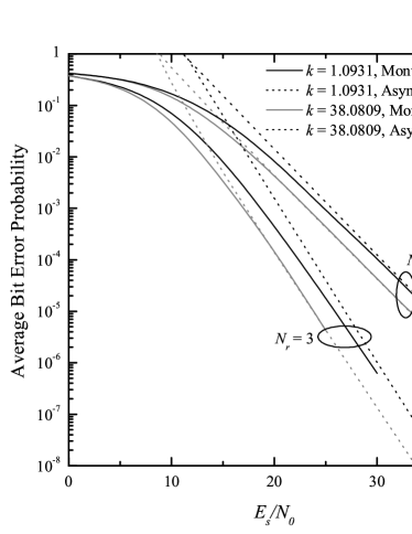
Numerical results accompanied by computer simulations are presented to study the tightness of (6) under various fading conditions. In the following analysis, an $8\times N_{r}$ MIMO system is considered. Fig. 1 depicts the ABEP of $8\times 2$ and $8\times 3$ MIMO SSK systems operating over EGK fading channels as a function of $E_{s}/N_{0}$, assuming $m_{s,i,\ell}=2$, $\beta_{s,i,\ell}=1$, $m_{i,\ell}=1.5$, $\beta_{i,\ell}=4$ and $\Omega_{i,\ell}\in\{1,5\}$. Fig. 1 includes upper bounds for the ABEP obtained by the numerical integration of (16), exact ABEP results obtained from Monte-Carlo simulation as well as asymptotic ABEP results obtained employing the high SNR assumption in (6) and (9). As it is evident, the proposed analytical framework well predicts the diversity and coding gains of the considered system and yields tight results for high values of $E_{s}/N_{0}$. Moreover, it can be observed that $\Omega_{i,\ell}$ affects coding gain only and, as expected, coding gain improves as $\Omega_{i,\ell}$ increases.

For the same antenna configurations, Fig. 2 depicts the ABEP of MIMO SM-QPSK $(M=4)$, operating over generalized-$\mathcal{K}$ fading channels as a function of $E_{s}/N_{0}$, assuming $m_{i,\ell}=1.5$, $\Omega_{i,\ell}=1$ and $m_{s,i,\ell}=k$. Different values of $k$ are considered to account for two shadowing scenarios, that is frequent heavy shadowing ($k=1.0931$) and average shadowing ($k=38.0809$) [16]. As for the tightness of (6), similar conclusions to those reported in Fig. 1 are deduced. However, in the presence of heavy shadowing ($k=1.0931$) and for $N_{t}=3$ transmit antennas, the asymptotic behavior of the ABEP-SNR curve shows up at high SNR values, i.e. for $E_{s}/N_{0}>30$dB. Furthermore, as it is expected, coding gain improves as $k$ increases, i.e. when the impact of shadowing becomes less severe.

IV Conclusion

In this letter, an analytical framework for the computation of the diversity and coding gains of SM systems over generalized fading channels was presented. To the best of the authors’ knowledge, the derived Eqs. (5), (9) and (11) are novel and can be simplified to some particular cases already reported. The newly derived simplified ABEP expressions require much less time for numerical evaluation compared to the exact ones, which require numerical integration. It was shown that, under generalized fading, the diversity gains of spatial and joint components of SM do not depend on the fading severity.

References

• [1] M. D. Renzo, H. Haas, A. Ghrayeb, S. Sugiura, and L. Hanzo, “Spatial Modulation for Generalized MIMO: Challenges, Opportunities, and Implementation,” Proc. IEEE, 2013.
• [2] M. D. Renzo, H. Haas, and P. Grant, “Spatial modulation for multiple-antenna wireless systems: a survey,” IEEE Commun. Mag, vol. 49, no. 12, pp. 182–191, Dec. 2011.
• [3] M. D. Renzo and H. Haas, “A general framework for performance analysis of Space Shift Keying (SSK) modulation for MISO correlated Nakagami-$m$ fading channels,” IEEE Trans. Commun., vol. 59, no. 9, pp. 2590–2603, Sep. 2010.
• [4] ——, “Space Shift Keying (SSK–) MIMO over correlated Rician fading channels: Performance analysis and a new method for transmit-diversity,” IEEE Trans. Commun., vol. 59, no. 1, pp. 116–129, Jan. 2011.
• [5] M. D. Renzo, H. Haas, and P. Grant, “Bit error probability of SM-MIMO over generalized fading channels,” IEEE Trans. Veh. Technol., vol. 61, no. 3, pp. 1124–1144, Mar. 2012.
• [6] K. Peppas, M. Zamkotsian, F. Lazarakis, and P. Cottis, “Unified error performance analysis of space shift keying modulation for MISO and MIMO systems under generalized fading,” IEEE Wireless Commun. Letters, vol. 2, no. 6, pp. 663–666, 2013.
• [7] M. D. Renzo and H. Haas, “Bit error probability of space modulation over Nakagami-$m$ fading: Asymptotic analysis,” IEEE Commun. Lett., vol. 15, no. 10, pp. 1026–1028, Oct. 2011.
• [8] Z. Wang and G. Giannakis, “A simple and general parametrization quantifying performance in fading channels,” IEEE Trans. Commun., vol. 51, no. 8, pp. 1389–1398, Aug. 2003.
• [9] A. D. Poularikas, The Transforms and Applications Handbook, 2nd ed.   CRC and IEEE Press, 2000.
• [10] I. Gradshteyn and I. M. Ryzhik, Tables of Integrals, Series, and Products, 6th ed.   New York: Academic Press, 2000.
• [11] F. Yilmaz and M.-S. Alouini, “A new simple model for composite fading channels: Second order statistics and channel capacity,” in Proc. (ISWCS), York, Sep. 2010, pp. 676 – 680.
• [12] A. P. Prudnikov, Y. A. Brychkov, and O. I. Marichev, Integrals and Series Volume 3: More Special Functions, 1st ed.   Taylor And Francis Ltd, 2003.
• [13] K. Peppas, F. Lazarakis, A. Alexandridis, and K. Dangakis, “Simple, accurate formula for the average bit error probability of multiple-input multiple-output free-space optical links over negative exponential turbulence channels,” Optics Letters, vol. 37, pp. 3243–3245, Aug. 2012.
• [14] F. Yilmaz and M.-S. Alouini, “Product of the powers of generalized Nakagami-$m$ variates and performance of cascaded fading channels,” in IEEE Global Telecommunications Conf., 2009, pp. 1 – 8.
• [15] T. Wolfram function site, [Online], available at http://functions.wolfram.com.
• [16] K. Peppas, “Accurate closed-form approximations to generalized-K sum distributions and applications in the performance analysis of equal gain combining receivers,” IET Commun., vol. 5, pp. 982–989, 2011.