Solitons and entanglement in the double sine-Gordon model

Abstract

The bipartite ground state entanglement in a finite linear harmonic chain of particles is numerically investigated. The particles are subjected to an external on-site periodic potential belonging to a family parametrized by the unit interval encompassing the sine-Gordon potential at both ends of the interval. Strong correspondences between the soliton entanglement entropy and the kink energy distribution profile as functions of the sub-chain length are found.

Introduction. - Entanglement in systems displaying solitonic solutions has been studied for some specific models Knoll 01 ; Lewenstein09 ; Carr09 ; Lee05 ; Partner13 . Recently, solitons in discrete chains presenting bounded internal modes have received increasing attention from both experimental and theoretical point of view Landa10 ; Landa13 ; Milenz13 ; Schneider12 ; Landa14 ; Ulm13 ; Ejtemaee13 ; Pyka13 . Since solitonic solutions of nonlinear models are characterized by being localized and topologically protected, investigation focusing on their use for quantum information tasks are in progress. As for example, in Marcovitch08 the authors studied the behavior of entanglement in a chain of particles using the Frenkel-Kontorova model FKmodel ; FKmodelB ; FK model 2 , and they have investigated the possibility to use solitons as the carrier of quantum information. In this model the particles of the 1-D chain interact by means of an elastic force with the nearest neighbors and are subjected to an on-site (substrate) sine-Gordon potential $V$. The strength of the elastic couplings $g$ between adjacent particles becomes a parameter in the model which rules the width (proportional to $\sqrt{g}$) of the unique soliton energy density lump. The influence of the sG soliton on the bipartite entanglement was analyzed by means of the von Neumann entropy, where one of two sub-blocks which conform the chain is always centered at the kink energy density maximum (kink center). The authors study the dependence of the von Neumann entropy on the size of the subblocks for several values of $g$, i.e., for several values of the soliton width. The result is that the presence of the soliton enhances the entanglement reaching a maximum when the size of the sub-block coincides approximately with the soliton width. The investigation of this issue in interacting multi-soliton solutions is achieved in Fujii08 .

Solitons and/or kinks are extended states whose energy densities are spatially localized in bounded regions in contrast with vacuum energy densities which are spatially homogeneous. In scalar field theory on the real line the existence of kinks comes from quantization of solitary wave solutions of the classical field equations. These traveling waves have energy densities showing one or several lumps of energy moving together with their center of mass. Thus, the kink center and the centers and widths of these lumps characterize the extended state, see e.g. Book Rajaranan . We shall address a system in this class determined by the family of double sine-Gordon potential energy densities:

$$V(\phi;a)=1-(1-a)\cos(2\pi\phi)-a\cos(4\pi\phi)\hskip 17.07182pt,\hskip 17.07182pta\in[0,1]\quad.$$

The family parameter $a$ is chosen to be in the unit interval in order to have a function $V$ semi-definite positive. At $a=0$ the standard sine-Gordon (sG) model is included, whereas at $a=1$ the sG model reappears although the argument is twice the standard sine-Gordon angle. Crucial to us in this work is the existence of kink traveling waves in any member of this family of models. The structure of the kink profiles, however, differs with varying values of $a$. In particular, in the range $0\leq a\leq\frac{1}{5}$ the kink energy density shows a single maximum at the kink center, i.e., it is formed by only one lump of energy density. In the range $\frac{1}{5}<a<1$, however, the kink energy density presents two separated maxima symmetrically distributed with respect to the kink center. The kink profile is formed by two separated energy density lumps if $a$ is greater than $\frac{1}{5}$ and less than $1$. The distance between the lump centers grows with $a$ and becomes infinity at $a=1$ where the one-lump sine-Gordon kink of double angle emerges, see References Alberto11 ; Campbell86 .

We shall work in the Frenkel-Kontorova scheme choosing as on-site substrate the potential of the double sine-Gordon model, i.e., we shall focus on the double sine-Gordon model defined on a finite chain of points instead of on the whole real line. Following the ideas disclosed in Marcovitch08 , we shall study soliton entanglement entropy replacing the standard sine-Gordon on-site potential by one potential belonging to the double sine-Gordon (dSG) family. By this token we enlarge the number of physical parameters. Besides the spring constant $g$, the family parameter $a\in[0,1]$ plays a significant r$\hat{{\rm o}}$le. The length where the kink energy density departs from the vacuum energy, the kink width, is proportional to $\sqrt{g}$ whereas $a$ determines the kink profile shape. These facts together make the dSG model specially suitable to investigate entanglement entropy when the kink energy distributions are more or less extended over the chain and/or their shape exhibits one or two energy lumps with different separations. With this in mind we divide the chain following Marcovitch08 into two complementary sub-blocks or sub-chains with no common points. Unlike Marcovitz et al. we select the two sub-chain starting from the two chain endpoints. We expect that the entanglement between fluctuations in different sub-chains will be influenced by how much of the kink energy distribution is contained in each sub-chain. The $g$ parameter leads us to distinguish three characteristic regimes: (1) First, we address the situation where the kink width is much shorter than the total chain length. For instance, the choice of $g=10^{4}$ on a chain of length $501$ points (used in this paper) the kink energy density occupies one fifth of the chain. The kink is clearly localized. (2) Second, in a chain of the same length a coupling of $g=10^{5}$ concentrates the kink in three fifths of the chain. The kink is more spread throughout the chain in this regime than in the previous one. (3) Third, choosing again the same chain but having $g=10^{6}$ we encounter the last regime: the kink energy distribution encompasses the whole chain. Clearly, similar regimes for longer chains are found for higher values of $g$. In all these considerations it is assumed that the kink center sits at the chain midpoint.

We shall perform numerical calculations of the correlation functions and the von Neumann entropy in these three regimes. Both the quantum vacuum and kink sectors will be investigated, whereas three values of the $a$ parameter will be considered distinguishing kink profiles with a single lump, two close lumps, and two widely separated lumps. Our results offer a refinement in several directions on the structure of the soliton entanglement entropy discussed in Marcovitch08 . First, the spatial correlation functions computed before the partition into two subchains show shapes in strong correspondence with the kink energy distribution profile. These correspondences are unveiled in the three regimes previously described, in each of them for the three characteristic values of $a$. Comparison with spatial correlation between vacuum fluctuations is also offered. In a second step, we use the knowledge of the correlation functions to compute, also numerically, the entanglement entropy arising in a partition of the system into two subchains between fluctuations living in different parts of the chain. Our $N$-particle chain will thus be divided into one $\ell$-particle and another $N-\ell$ particle subblock with all the $\ell$ points in the first subchain located at the left of the $N-\ell$ points of the second subchain. We shall compute the entanglement for different choices of the partition length $\ell$. The main conclusion is that entanglement between fluctuations in the two different subchains is maximum when $\ell$ coincides with one of the kink lump centers. If the kink energy density shows two energy lumps the entanglement entropy as a function of $\ell$ reaches two maxima too precisely when the length of the subblock $\ell$ coincides with the kink lump centers. In more general terms, we claim that the entanglement is enhanced when the kink energy density at the sub-block endpoint increases and it is maximum when the kink energy density is maximum.

Quantization. - We shall address a 1-D linear harmonic chain of $N$ particles interacting with the nearest neighbors and subjected to an on-site (substrate) potential $V$. We assume that the equilibrium position of the $n$-th particle in the chain is $X_{n}^{V}=n$, $n=0,\dots,N$. The classical Hamiltonian governing the dynamics of this model is

$$H=\sum_{n=0}^{N-1}\,{\cal H}_{n,n+1}=\sum_{n=0}^{N-1}\frac{1}{2}\left[\pi_{n}^{2}+2V(\phi_{n})+g(\phi_{n+1}-\phi_{n})^{2}\right].$$ (1)

where $\phi_{n}$ represents the displacement of the $n$-th particle with respect to its equilibrium position, $X_{n}=n+\phi_{n}$, $\pi_{n}=\dot{\phi}_{n}$ is the momentum of the $n$-th particle, $g$ is the non dimensional strength of the elastic couplings between adjacent neighbor particles, and $V$ represents the external on-site potential, see FKmodel . We assume that $V(\phi)$ is a non negative function which vanishes when the displacements reach an equilibrium point. In formula (1) all the magnitudes involved, particle positions, momenta, and potential are rescaled to non dimensional quantities. The system of coupled ODE’s

$$\frac{d^{2}\phi_{n}}{dt^{2}}=-\frac{\partial V(\phi_{n})}{\partial\phi_{n}}+g(\phi_{n+1}-2\phi_{n}+\phi_{n-1})\,\,\,,\hskip 28.45274ptn=0,1,\dots,N$$ (2)

are the equations of motion describing the classical dynamics of the model, whereas time-independent solutions are determined from the difference equations system:

$$-\frac{\partial V(\phi_{n})}{\partial\phi_{n}}+g(\phi_{n+1}-2\phi_{n}+\phi_{n-1})=0\hskip 28.45274pt.$$ (3)

We shall distinguish two types of time-independent finite energy solutions:

1. Homogeneous solutions of (3), denoted as $\phi^{{\rm V}}(n)=\phi_{n}^{{\rm V}}$:

   $$\phi^{{\rm V}}(n)=\phi_{n}^{{\rm V}}=0\hskip 14.22636pt\mbox{with}\hskip 14.22636ptn=0,1,\cdots,N\,\,\,.$$

   All the particles sit at their equilibrium points $X_{n}=n$ in such a way that their classical energy is zero: $H(\phi_{n}^{{\rm V}})=0$. We shall refer to them as vacuum solutions foreseeing future treatment in a quantum setting.

2. Discrete soliton/kink solutions, which we shall denote as: $\phi_{n}^{S}=\phi^{S}(n)$. Soliton and kink are frequently used as synonymous in the Literature. The strict concept of soliton, however, is more restrictive. Both kinks and solitons are solitary non-linear waves, but they differ in the fact that solitons preserve shapes after collisions. We shall denote as kinks the non-homogeneous solutions from now on throughout this paper. Kinks are thus solutions of (3) obeying the following boundary conditions:

   $$\phi^{S}(0)=\phi_{0}^{S}=0\hskip 28.45274pt,\hskip 28.45274pt\phi^{S}(N)=\phi_{N}^{S}=1\,\,,$$ (4)

   characterized accordingly by the non null “topological charge”: $T=|\phi_{N}^{S}-\phi_{0}^{S}|=1$. The boundary conditions (4), tantamount to $X_{0}^{S}=0$ and $X_{N}^{S}=N+1$, demand that the kink profile will depart from the particle equilibrium positions somewhere in the middle of the chain. The kink energy distribution (density in the continuum limit) is: ${\cal E}(\phi_{n}^{S})=V(\phi_{n}^{S})+\frac{1}{2}g(\phi_{n+1}^{S}-\phi_{n}^{S})^{2}$.

Small fluctuations $\eta(n,t)$ around static solutions $\phi^{{\rm sta}}(n)=\phi_{n}^{{\rm sta}}$, either vacuum or kink configurations,

$$\phi(n,t)=\phi_{n}^{{\rm sta}}+\eta(n,t)$$

are still solutions of the ODE’s system (2) if and only if the following ODE’s linear system

$$\Big{(}\frac{d^{2}}{dt^{2}}+\Omega(n)+2g\Big{)}\eta(n,t)-g\,\eta(n-1,t)-g\,\eta(n+1,t)={\cal O}(\eta^{2})$$ (5)

is satisfied, see Alberto11 . In formula (5) $\Omega$ is the second derivative of the potential evaluated at the static solution:          $\Omega(n)=\frac{d^{2}V}{d\phi^{2}}\left[\phi_{n}^{{\rm sta}}\right]$.

If $\phi_{n}^{{\rm sta}}=\phi_{n}^{V}$ then $\Omega(n)$ is the curvature of the potential at the equilibrium points, where all the particles of the chain sit. If $\phi_{n}^{{\rm sta}}=\phi_{n}^{S}$ then $\Omega(n)$ is evaluated at kink solutions and because kinks are not homogeneous, i.e., they vary with $n$, it takes different values at different points of the chain. From the spectral problem of the $(N+1)\times(N+1)$ Hessian matrix $B(n,m)$

$$B(n,m)=\Big{(}\Omega+2g\Big{)}\delta_{nm}-g\,\delta_{n,m-1}-g\,\delta_{n,m+1}\,\,\,,\,\,\,\,\,\sum_{m=0}^{N}B(n,m)\psi_{k}(m)=\omega_{k}^{2}\psi_{k}(n)$$ (6)

where $\Omega$ obeys to either to vacuum or kink static solutions, the general solution of the ODE’s system (5)

$$\eta(n,t)=\sum_{k=0}^{N}\,\frac{1}{\sqrt{2\omega_{k}}}\left(a_{k}\,e^{i\omega_{k}t}+a_{k}^{*}\,e^{-i\omega_{k}t}\right)\psi_{k}(n)$$ (7)

is obtained in terms of the $(N+1)$ normal modes of fluctuation $\psi_{k}(n)$, whose eigenvalues have been denoted as $\omega_{k}^{2}$, see (6). Dirichlet boundary conditions ensure that the eigenmodes are real.

Quantization of this pre-quantum picture is achieved by promoting the $a_{k}$ and $a_{k}^{*}$ coefficients to annihilation and creation bosonic operators: $[\widehat{a}_{k}^{\dagger},\widehat{a}_{q}]=\delta_{kq}$. The bosonic quantum field and its conjugate momenta operator read:

$$\widehat{\eta}(n,t)=\sum_{k=0}^{N}\frac{1}{\sqrt{2\omega_{k}}}\,\left(\widehat{a}_{k}\,e^{i\omega_{k}t}+\widehat{a}_{k}^{\dagger}\,e^{-i\omega_{k}t}\right)\psi_{k}(n)\,\,\,,\,\,\,\,\,\widehat{\pi}(n,t)=i\sum_{k=0}^{N}\sqrt{\frac{\omega_{k}}{2}}\,\left(\widehat{a}_{k}\,e^{i\omega_{k}t}-\widehat{a}_{k}^{\dagger}\,e^{-i\omega_{k}t}\right)\psi_{k}(n)\,\,.$$ (8)

States characterized by a set of occupation numbers $n_{k}$ of each $k$-th normal mode are eigenfunctions of the linearized Hamiltonian $\widehat{H}_{0}=\sum_{k=0}^{N}\,\left(\widehat{a}^{\dagger}(k)\widehat{a}(k)+\frac{1}{2}\right)\omega_{k}$ of energy:

$$\widehat{H}_{0}|\left\{n_{k}\right\}\rangle=E_{\left\{n_{k}\right\}}|\{n_{k}\}\rangle\quad,\quad E_{\left\{n_{k}\right\}}=\sum_{k=0}^{N}\left(n_{k}+{\textstyle\frac{1}{2}}\right)\omega_{k}\,\,.$$ (9)

These Fock space states correspond to the fundamental mesons of the system, both in the vacuum sector and in the kink sector, distinct alternatives distinguished by the appropriate choice of the $B$ matrix.

The double sine-Gordon model.- We choose the substrate potential between the members of the one-parametric family of double sine-Gordon (dSG) potentials

$$V(\phi;a)=1-(1-a)\cos(2\pi\phi)-a\cos(4\pi\phi)\,\,\,,\,\,\,a\in[0,1]\,,$$ (10)

plotted in Figure 1 as a function of $\phi$ for three characteristic values: $a=0.0$, $0.6$ and $0.99$, see Mussardo07 .

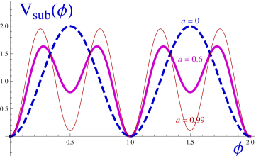
Figure 1: Double sine-Gordon potential for the parameters $a=0.0$ (blue dashed line), $0.6$ (pink thick solid line) and $0.99$ (red thin line).

The set of absolute minima or zeroes of $V(\phi;a)$ in the interval $a\in[0,1)$ is independent of $a$: ${\cal M}=\{\phi^{(j)}=j\,\,,\,\,j\in\mathbb{Z}\}$, see Figure 2. As a function of $\phi$ (10), however, exhibits more critical points. $\frac{dV}{d\phi}(\phi;a)=0$ if and only if:

$$\phi^{(j)}=j\quad,\quad\phi^{(j+\frac{1}{2})}=j+\frac{1}{2}\quad,\quad\phi^{(\pm,\,j)}=\pm\frac{1}{\pi}{\rm arctan}\sqrt{\frac{3a+1}{5a-1}}+j\quad.$$ (11)

Evaluation of the second derivative of the potential at the three types of critical points

$$\frac{d^{2}V}{d\phi^{2}}(0;a)=4(1+3a)\pi^{2}\hskip 11.38092pt,\hskip 11.38092pt\frac{d^{2}V}{d\phi^{2}}({\textstyle\frac{1}{2}};a)=4(5a-1)\pi^{2}\hskip 11.38092pt,\hskip 11.38092pt\frac{d^{2}V}{d\phi^{2}}(\phi^{(+,0)};a)=\frac{1-a(2+15a)}{a}\pi^{2}$$ (12)

tells us that the first type is always formed by minima of $V$, the second type contains maxima if $a<\frac{1}{5}$ that become relative minima when $a$ reaches $\frac{1}{5}$ and the last type formed only by real critical points for $a>\frac{1}{5}$ that are always maxima, see Figure 1 and 2. Only quantization over absolute minima is safe, relative minima give rise to false vacua through tunnel effects, and maxima produce tachyons. We thus choose the state with no fluctuations over the classical configuration $\phi^{(0)}$ as the vacuum state of the quantum system . Quasi-particles of mass $4(1+3a)\pi^{2}$ arise when the creation operator $\hat{a}^{\dagger}$ acts on the vacuum state.

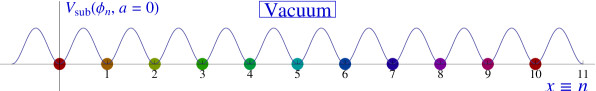
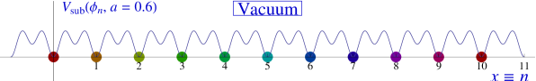
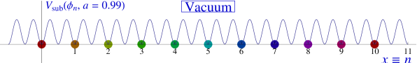
Figure 2: Pictures of vacuum solutions for a chain of 11 particles subjected to a double sine-Gordon substrate potential, corresponding to the $a$ parameter values: (a) $a=0.0$, (b) $a=0.6$ and (c) $a=0.99$.

Besides the homogeneous solutions of the field equations (3) listed in (11) there are other static but $n$-dependent solutions in these model. These are the kinks that must comply with the contour conditions (4) at the endpoints because the system is defined on a finite chain, see Figure 3.

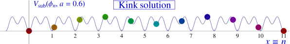
Figure 3: Graphics of the kink solution numerically obtained for a chain of 11 particles under the dSG substrate potential and the parameter value: $a=0.6$. Note that the particle on the right boundary is displaced in one site with respect to the same particle in the vacuum. The particles not in the boundary are displaced away from their equilibrium positions.

The system of finite differences equations (3) shows that these solutions depend both on $a$ and the strength of the elastic coupling $g$. As stated before the parameter $g$ rules the extension of this topological solution along the chain, see Marcovitch08 . A qualitative analysis of (3) confirms this claim. If $g$ is strong enough the particle distribution solving (3) is such that $\phi_{n+1}-\phi_{n}\simeq\frac{1}{N}$ for almost all $n$. $\phi(n)$ is almost a straight line with a slope as small as allowed by the boundary conditions. The influence of the external potential is very small and the kink profiles depart from the homogeneous vacuum practically along the whole chain. At weak coupling $g\rightarrow 0$, however, the distribution of particles favoured by kink solutions of (3) presents abrupt changes from one to the next particle somewhere in the middle of the chain. The potential provides strong forces away the thin kink region restoring the particles to lie on consecutive absolute minima of $V$ at the two sides of the kink. In this case the effect of the kink is confined within a small part of the chain. In Figures 4-5-6 we show graphics of numerically generated kink solutions with unit topological charge for several values of the elastic constant $g$ in a chain of $N+1=501$ particles together with their energy distributions where the above mentioned pattern is observed. Having fixed this length for the chain we have selected two values of $g$ in order to characterize the strong and weak regimes mentioned above plus one third value in between to analyze the intermediate regime. It is clear that for chains of different length one must adopt other values of $g$ to deal with kinks that cover $\frac{1}{5}$, $\frac{3}{5}$, and/or the whole chain. We thus distinguish three different regimes:

1. Substrate potential dominant regime (SubsReg). We select the value $g=10^{4}$ as the regime representative in a $N=500$ particle chain. The dynamics is fundamentally determined by the substrate potential in detriment of the elastic inter-particle forces. The kink energy distribution is localized in an interval of length $\frac{N}{5}=100$.

2. Balanced Substrate potential/Elastic force regime (BalReg). $g=10^{5}$ is the representative value of the elastic parameter in a chain of the same length. Elastic forces and those induced by the substrate potential act on each particle in a balanced manner. Under these circumstances the kink energy distribution spreads on an interval of length $3\frac{N}{5}=300$.

3. Elastic force dominant regime (ElasReg). On the same chain $g=10^{6}$ is a representative value of this third regime. Forces induced by the substrate potential are very weak as compared with the elastic interparticle forces. The kink energy distribution is smoothly distributed over the whole chain.

   

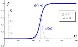
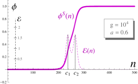
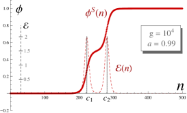
Figure 4: Kink profiles (solid line) and their energy distributions (dashed line) for $a=0$, $a=0.6$ and $a=0.99$ in the substrate potential dominant regime of the dSG model on a $N=500$ chain. The kink profiles jump from a homogeneous solution to the next one in a abrupt manner. Accordingly, the kink energy distributions neatly depart from zero only on a short interval and have one maximum if $a<\frac{1}{5}$ but two maxima appear if $a>\frac{1}{5}$.

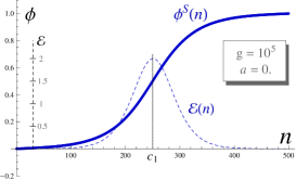
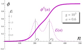
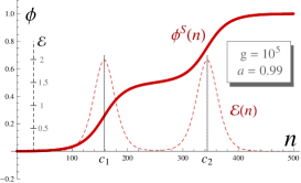
Figure 5: Kink profiles (solid line) and their energy distributions (dashed line) for $a=0$, $a=0.6$ and $a=0.99$ in the balanced substrate potential/elastic force regime of the dSG model on a $N=500$ chain. The jump from a vacuum solution to the next one is less steep than in the regime discussed in Figure 4. The kink energy distributions are also less localized and spread over longer intervals. The distinct number of lumps, one if $a<\frac{1}{5}$, two for $a>\frac{1}{5}$, is also observed.

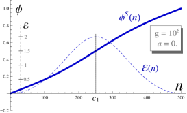
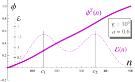
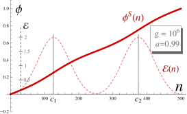
Figure 6: Kink profiles (solid line) and their energy distributions (dashed line) for $a=0$, $a=0.6$ and $a=0.99$ in the elastic force dominant regime of the dSG model on a $N=500$ chain. The kink profiles climb almost uniformly starting from one vacuum solution at the chain left endpoint and ending at the next vacuum solution on the chain right endpoint. The kink energy distributions are even less localized than those in the previously described regime. The existence of energy distributions formed by one or two lumps when $a$ is below or above $\frac{1}{5}$ is also appreciated.

In sum, the set of graphics displayed in Figures 4-5-6 reveals the r$\hat{{\rm o}}$le of the parameter $a$. For $a$ less than but close to one the kink profile consists in a two-step climbing, with a long plateaux in between, from one vacuum solution up to the next one. The energy distribution is concentrated around the midpoints of each jump and thus a two energy lump configuration arise. The reason is the existence of a relative minima of $V$ between each two absolute minima when $a>\frac{1}{5}$, recall formulas (11) and (12). Moreover, because $V(\phi^{{(j+\frac{1}{2})}})=2(1-a)$ the value of the potential at these relative minima is close to zero when $a$ is slightly less than one. The climb from $\phi^{(j)}$ to $\phi^{(j+1)}$ “resting”at $\phi^{(j+1/2)}$ as much as possible. Thus, the distance between the two jumps is very large when, e.g., $a=0.99$. When $a$ decreases but is still greater than $\frac{1}{5}$ the situation is the same but the value of the potential at the relative minimum is higher and the distance between the jumps is shorter, i.e., the two lumps in the energy distribution are closer. Finally, if $a<\frac{1}{5}$ the relative minima become maxima and the climbing takes place in one step because there is no a relative minima in between to rest. The $a=1$ limit is special. The relative minima become absolute, zeroes of the substrate potential $V(\phi;1)$, that form the set: ${\cal M}(1)=\{\phi^{{(j)}}={\textstyle\frac{j}{2}}\,\,,\,\,j\in\mathbb{Z}\}$. For this value the dSG potential (10) becomes a pure sG potential again. Certainly the model in the limit $a=1$ involves a two-kink solution of a single-well sine-Gordon potential with argument twice the usual angle. In the field theory model on the continuous real line this limit implies that one of the kinks goes to infinity because the relative minimum becomes absolute. In a finite discrete chain, we selected the value $a=0.99$ to offer a description of kink profiles close to this limit: the two lumps of energy moves towards the endpoints of the chain.

At this point, it is important to emphasize that the surge of two lumps on kink profiles when $a>\frac{1}{5}$ in the unit topological charge sector of the double sine-Gordon does not means that these soliton structures are multi-soliton or breather solutions akin to those arising in pure sine-Gordon models, i.e., the models found in the boundary points $a=0$ and $a=1$ of the family. sine-Gordon multisolitons live in sectors with topological charge different from one and are time-dependent even in their center of mass. Unlike in the standard sine-Gordon model, there exists forces between kinks either formed by one or two lumps in the double sine-Gordon models, specifically between kinks and anti-kinks, see Campbell86 . Isolated kinks, however, are static in their center of mass: either formed by one or two lumps the only time-dependence arise from the motion of the center of mass obeying to Lorentz transformations.

We pass to study how the rich structure of these dSG solitons influences quantum entanglement between vacuum and kink fluctuations. In particular, we begin by analyzing the spatial correlation functions between two particles in the chain in the kink and vacuum sectors.

Spatial Correlation Functions. - To compute spatial correlation functions in this $N$-particle system we follow the procedure established in the References Simon94 ; Marcovitch08 . The canonical variables are assembled into a vector $Y=(\eta,\pi)$ which is a point in phase space. The $N$-component vectors $\eta=(\eta_{1},\eta_{2},...,\eta_{N})$ and $\pi=(\pi_{1},\pi_{2},...,\pi_{N})$ encompass respectively the particle positions and momenta. Quantization forces the following commutation rules:

$$[\widehat{Y}_{\alpha},\widehat{Y}_{\beta}]=iJ_{\alpha\beta}\quad,\quad J=\left(\begin{array}[]{cc}\mathbf{0}&\mathbf{1}\\ -\mathbf{1}&\mathbf{0}\end{array}\right),$$ (13)

where the $2N\times 2N$ symplectic matrix $J$ is written in this formula as $N\times N$ blocks of the null and identity matrices. Expectation values of two canonical variables in a quantum state are the matrix elements of the $2N\times 2N$ covariance matrix $M={\rm Re}[\langle\widehat{Y}\widehat{Y}^{T}\rangle]$, which may be diagonalized in the Williamson form $W=S_{W}MS_{W}^{-1}={\rm diag}\left(\lambda_{1},\lambda_{2},...\lambda_{N},\lambda_{1},\lambda_{2},...\lambda_{N}\right)$, where the eingenvalues $\lambda_{j}\geq\frac{1}{2}$ are the moduli of the eigenvalues of the matrix $JM$. Gaussian states are completely characterized by the covariance matrix $M$ and by their first momenta. Partitioning the N-mode system into two sets $A$ and $B$, the reduced covariance matrices $M_{k}={\rm Re}[\langle\widehat{Y}_{k}\widehat{Y}_{k}^{T}\rangle]$, $k=A,B$, must be put in the Williamson form. Matrix elements of the covariance matrix $M$ are thus of the form $\left\langle\hat{\eta}(n)\hat{\eta}(m)\right\rangle={\rm tr}\,\hat{\rho}\hat{\eta}(n)\hat{\eta}(m)$, $\left\langle\hat{\pi}(m)\hat{\eta}(n)\right\rangle={\rm tr}\,\hat{\rho}\,\hat{\pi}(m)\hat{\eta}(n)$ and $\left\langle\hat{\pi}(n)\hat{\pi}(m)\right\rangle={\rm tr}\,\hat{\rho}\,\hat{\pi}(n)\hat{\pi}(m)$, where $\hat{\rho}$ is the density operator of the quantum state of the chain and $\hat{\eta}(n)$, $\hat{\pi}(n)$ are the quantum operators defined in (8). Assuming that the whole system is in the ground state we find the correlation functions between particle positions and momenta

$${\rm Re}\left\{\langle\widehat{\eta}(m)\widehat{\eta}(n)\rangle\right\}=\frac{1}{2}\sum_{l}\frac{\psi_{l}(m)\psi_{l}(n)}{\omega_{l}}\hskip 14.22636pt,\hskip 14.22636pt{\rm Re}\left\{\left\langle\widehat{\pi}(m)\widehat{\pi}(n)\right\rangle\right\}=\frac{1}{2}\sum_{l}\omega_{l}\psi_{l}(m)\psi_{l}(n)\,\,\,,$$ (14)

whereas positions and momenta verify: ${\rm Re}\left\{\langle\widehat{\pi}(m)\widehat{\eta}(n)\rangle\right\}={\rm Re}\left\{\left\langle\widehat{\eta}(m)\widehat{\pi}(n)\right\rangle\right\}=0$.

Correlations between two particle positions are obtained from the normal modes eigenvalues and eigenfunctions:

$$\xi_{mn}=\left\langle\widehat{\eta}({\textstyle m})\,\widehat{\eta}(n)\right\rangle=\frac{1}{2}\sum_{k=0}^{N}\frac{\psi_{k}(m)\psi_{k}(n)}{\omega_{k}}\quad.$$ (15)

In Figures 7 (a)-(b)-(c) the dependence on $n$ of the spatial correlation function when one of the particles sits at the left endpoint of the chain $\xi_{0n}=\xi_{n}$ is displayed. Numerical computations relying on formula (15) have been performed for our chain of $501$ particles, accounting for vacuum and kink normal modes, in the nine cases where the kink profiles were depicted: three characteristic values of $a$ and $g$. The properties of correlation functions as functions of $n$ are clearly observed in the $g=10^{4}$ regime. Vacuum and kink correlations $\xi_{n}$ do not differ from each other for small $n$ where the kink profile does not depart too much from the vacuum solution. At larger $n$ kink fluctuation correlations remarkably grow bigger than vacuum correlations until reaching one or two maximum values, precisely at the points where the kink energy distribution also reaches its maximum values. If $n_{+}$ denotes the position of the maximum farther away from the origin, kink correlations start to decrease for $n>n_{+}$. The difference between kink correlations for $a<\frac{1}{5}$ and $a>\frac{1}{5}$ is that in the first case there is only a single maximum $n_{0}$ whereas there are two $n_{\pm}$ if $a>\frac{1}{5}$. Kink correlations in the last case decrease after $n_{-}$, pass a relative minimum at $n_{0}$, and increase again up to $n_{+}$, see Figure 7(a). We conclude that two-point particle spatial correlations in the kink sector recognize somehow the kink profile shape. This behavior, albeit less pronounced, is reproduced in the BalReg regime, Figure 7(b), whereas in the ElasReg regime, see Figure 7(c), the curvatures at the maxima are very mild and the correlation functions $\xi_{n}$ for vacuum and kink fluctuations look similar. We thus conclude that the logarithmic correlations in the kink sector behave in a remarkable different manner that vacuum correlations of standard logarithmic class: $\xi_{mn}^{V}=\log\frac{1}{|m-n|}$.

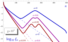
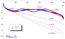
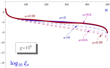
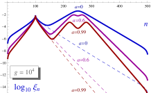
Figure 7: Graphics of the logarithmic correlation functions between two particles separated by $n$ positions for vacuum (dashed lines) and kink (solid lines) fluctuations. Plots of the correlation functions when one of them is located at the left endpoint of the chain: (a) SubsReg, (b) BalReg and (c) ElasReg regimes. In each regime, the parameter values $a=0$, $a=0.6$, and $a=0.99$ have been considered. (d) Graphics of the logarithmic correlation functions between the $m=100$th particle and a second one separated by $n$ positions for vacuum (dashed lines) and kink (solid lines) fluctuations in the $g=10^{4}$ SubsReg regime. The three characteristic values $a=0$, $a=0.6$, and $a=0.99$ have been considered.

The correlation function shapes as functions of the interparticle distance just described follows a similar pattern independently of the fixed particle position. In order to illustrate this fact, correlation functions between the $m=100$th particle and a second particle located in an arbitrary point $m+n$ of the $N=500$ chain are displayed in Figure 7 (d) for $g=10^{4}$. Neither the kink configuration nor the contour conditions affect the position of the fixed particle in the correlation function. Recall that the kink profile in this regime is confined approximately in the range $(200,300)$. We observe that the correlation function increases when the second particle position $100+n$ is located at the centers of the kink lumps. In comparison with the correlations between two particles located respectively at $0$ and $n$ this effect is reinforced because the fixed particle is closer to the kink center, see Figures 7a and 7d.

Entanglement. - Entanglement between fluctuations supported by Gaussian states is measured by taking advantage of the correspondence between the diagonal form of the covariance matrix $M={\rm Re}\left[\langle YY^{T}\rangle\right]$ for the Gaussian state with the covariance matrix of a thermal state, also diagonal in Fock space, having an average phonon number $\overline{n}_{j}=\lambda_{j}-\frac{1}{2}$ Simon94 . Here the $\lambda_{j}$ are the Williamson eigenvalues of the covariance matrix and entanglement entropy is accordingly defined as:

$$E_{S}=\sum_{j}S(\lambda_{j})\hskip 14.22636pt\mbox{with}\hskip 14.22636ptS(\lambda)=\left(\lambda+{\textstyle\frac{1}{2}}\right)\ln\left(\lambda+{\textstyle\frac{1}{2}}\right)-\left(\lambda-{\textstyle\frac{1}{2}}\right)\ln\left(\lambda-{\textstyle\frac{1}{2}}\right).$$ (16)

After choosing a subblock of $\ell$ particles forming a subchain $A$ of the whole chain of $501$ particles the eigenvalues of the reduced $2\ell\times 2\ell$ covariance matrix to this subblock are numerically computed. Formula (16) is then used to estimate also numerically the entanglement entropy. In contrast with the usual choice predominant in the Literature where the subchain is centered at the chain mid point, see e.g. Reference Marcovitch08 , we take the subblock starting from the left endpoint of the chain, see Figure 8. The reason is that performing these calculations on subchains of fixed but arbitrary length $\ell\leq 501$ a striking similarity between the entanglement entropy as a function of $\ell$ and the kink energy distribution along the chain clearly emerges. More precisely: entanglement between fluctuations in the sub-chains $A$ and $B$ is maximum when $\ell$ is chosen at a maximum of the kink energy distribution.

In Figures 9-10-11 the entanglement entropies numerically obtained from (16) are displayed corresponding to the three regimes where the kink profiles were shown before: SubsReg (Figure 9(a)-(b)-(c)), BalReg (Figure 10(a)-(b)-(c)), and ElasReg (Figure 11(a)-(b)-(c)). In each regime the graphics for the three values of $a$, $a=0$, $a=0.6$, and $a=0.99$, are depicted.

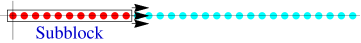
Figure 8: A subblock of particles attached to the left endpoint of the total chain.

Entanglement entropies between vacuum fluctuations depend only slightly on the subchain location. For fixed $g$ and $a$ they vary with $\ell$ in the same qualitative way as those entropies found for centered subchains. The differences are only quantitative: the heights of the plateau of these functions are smaller in this new location of the subblock. Kink fluctuation entanglement entropies require a much more detailed analysis. We shall describe in turn the results in the nine different cases:

A. Substrate potential dominant regime

The numerically computed entanglement entropy is displayed in Figures 9(a)-(b)-(c) for the three habitual values of the $a$ parameter. The kink energy distributions are also shown as a shadowed zone in the same Figures. Note the correspondence between the maxima of the kink energy distributions and the entanglement entropy as functions of $\ell$, in concordance also with the spatial correlation function maxima.

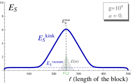
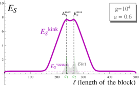
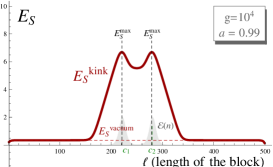
Figure 9: Entanglement entropy between kink-kink (solid line) and vacuum-vacuum (dashed line) fluctuations for: (a) $a=0$, (b) $a=0.6$ and (c) $a=0.99$ in the SubsReg regime $g=10^{4}$. The kink energy distributions are plotted as curves enclosing a shadowed area in the scale set by $E_{S}$. Dashed vertical lines have been included to point out the relative positions of the kink energy distribution and entanglement entropy maxima.

We remark the following facts: (1) For sine-Gordon kinks, $a=0$, the entanglement entropy between kink-kink and vacuum-vacuum fluctuations are identical when the subblock length $\ell$ is small. The kink supported entropy $E_{S}^{{\rm kink}}$ begins to increase and starts to differ from $E_{S}^{{\rm vacuum}}$ when $\ell$ approaches 150. The kink entanglement entropy reaches its maximum value at a subblock length of $\ell=250$. From this point onwards $E_{S}^{{\rm kink}}$ decreases until a subblock length of approximately $\ell=350$, a point where again the kink supported entropy equals the vacuum entropy, see Figure 9(a). The maximum of the entanglement entropy and the center of the kink energy distribution are identical and lie at the mid point of the chain, a fact shown by the vertical dashed line. The kink entanglement entropy is maximum for a subchain whose endpoint coincides with the kink energy distribution maximum point. Again this is in concordance with the spatial correlation function, which reaches its maximum just at the center of the single kink, see Figure 7.

(2) When $a=0.6$ the entanglement entropy between kink fluctuations behaves in a slightly different way. Like in the previous case $E_{S}^{{\rm kink}}$ fits in the function $E_{S}^{{\rm vacuum}}$ approximately until $\ell=150$. For subblocks of length $150<\ell<236$ the kink fluctuation entropy increases and reaches a maximum at $\ell=236$, precisely the center of the first lump of the kink energy distribution. The entropy of subchains of lengths in the interval $\ell\in(236,250)$ decreases until hitting a relative minimum $\ell=250$, half the whole chain length. Beyond this length the entanglement entropy between kink fluctuations starts to increase again reaching a second maximum at the center of the second lump of the kink energy distribution $\ell=264$. For subblock lengths in the interval $264<\ell<350$, $E_{S}^{{\rm kink}}$ decreases until approximately $\ell=350$. Beyond this subblock length the kink fluctuation entropy coincides again with $E_{S}^{{\rm vacuum}}$, see Figure 9(b).

(3) If $a=0.99$ the entanglement entropy $E_{S}^{{\rm kink}}$ follows the same pattern explained in the previous case, see Figure 9(c). Here the distance between the two maxima of the entanglement entropy is greater than the distance between the maxima of the $a=0.6$ kink. The positions of the two maxima occur in this case for subblock lengths: $\ell=221$ and $\ell=279$, the maxima of the kink energy distribution. The kink fluctuation entropy exhibits a relative minimum between the two maxima but the value of the kink entropy at this minimum is much greater than $E_{S}^{{\rm vacuum}}$ in the same range.

In the three cases the kink entanglement entropies and energy distributions are curves as functions of $\ell$ with similar shapes and only the scales are different. One also checks that the correlations functions in Figure 7(a)-(d) have the same critical points than the kink energy distributions.

B. Balanced Substrate potential-Elastic force Regime.

In Figures 10(a)-(b)-(c) graphics of both the entanglement entropy between vacuum-vacuum and kink-kink fluctuations in a $N=500$ particle chain are shown within the BalReg Regime $g=10^{5}$ for $a=0$, $a=0.6$ and $a=0.99$.

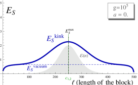
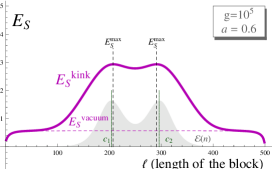
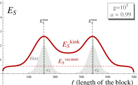
Figure 10: Entanglement entropies between kink-kink (solid line) and vacuum-vacuum (dashed line) fluctuations for: (a) $a=0$, (b) $a=0.6$ and (c) $a=0.99$ in the BalReg regime. The kink energy distributions are plotted as curves enclosing a shadowed area using the scale set by $E_{S}$. Dashed vertical lines show the relative positions of the maxima of the kink energy distribution and entanglement entropy.

There are only quantitative discrepancies with respect to the pattern just described in the previous $g=10^{4}$ regimes. The curves in this $g=10^{5}$ regime are smoother and consequently the differences between the $E_{S}^{{\rm kink}}$ and $E_{S}^{{\rm vacuum}}$ entropies are less pronounced than those occurring for $g=10^{4}$. The centers of the kink energy distributions, however, slightly differ from the maxima of $E_{S}^{{\rm kink}}$ both in the cases when the kink is formed by one or two lumps. More precisely: (1) For $a=0$ the entropy $E_{S}^{{\rm kink}}$ shows a maximum at the midpoint of the chain where the kink center is localized. (2) If $a=0.6$ the function $E_{S}^{{\rm kink}}$ exhibits two maxima situated at $\ell=207$ and $\ell=291$, and, despite that the respective maxima do not exactly coincide the kink entanglement entropy and the energy distribution have similar shapes as functions of $\ell$. (3) For $a=0.9$, the lengths of the subblocks for which the entanglement entropy is maximum are $\ell=157$ and $\ell=342$. This means that two subblocks which remarkably differ in length support maximum entropy. The lump centers nearly coincide with the entanglement entropy maxima. The little discrepancies between entropy and kink energy maxima are due to discreteness effects: the kink energy distribution is more extended in the chain than in the previous SubsReg regime and the location of the energy distribution maximum on a discrete chain is less accurate. In Figure 7(b) one observes that the spatial correlation functions give a clue of the entanglement entropy shapes also in this regime as one can check in Figures 10(a)-(b)-(c).

C. Elastic force dominant regime.

In Figures 11(a)-(b)-(c) the graphics of the entanglement entropies between kink-kink and vacuum-vacuum fluctuations are plotted in the $g=10^{6}$ ElasReg Regime for the three usual representative values of the parameter $a$.

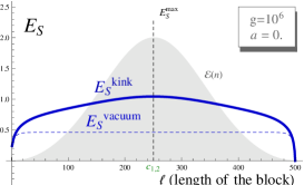
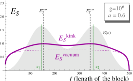
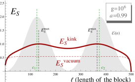
Figure 11: Entanglement entropies between kink-kink (solid line) and vacuum-vacuum (dashed line) fluctuations for: (a) $a=0$, (b) $a=0.6$ and (c) $a=0.99$ in the ElasReg regime. The kink energy distributions are plotted as curves enclosing a shadowed area using the same scale as $E_{S}$. Dashed vertical lines show the relative positions of the kink energy distribution and the entanglement entropy maxima.

Differences between kink-kink and vacuum-vacuum fluctuation entanglement entropies become small in this regime. In general, these differences get smaller when the elastic constant $g$ increases and the kinks become less concentrated. Nevertheless, the shape of the kink entropy and energy distribution keeps correlated, despite that the center of the kink energy distribution differs from the maxima of $E_{S}^{{\rm kink}}$ for $a=0.6$ and $a=0.9$ as in the BalReg regime. These discrepancies are not only due to discreteness effects. Contour effects also affect because the kink profile differs from a vacuum solution practically along the whole chain and the boundaries have a stronger influence on the kink energy distributions. In fact, notice that in this regime the kink loses its characteristic smooth staircase shape adopting an almost linear profile, see Figure 6. We remark three points: (1) The function $E_{S}^{{\rm kink}}$ exhibits a single maximum at the middle of the chain if $a=0$ as in the other two regimes previously discussed. (2) For $a=0.6$ the kink fluctuation entropy exhibits two low curvature maxima at the values $\ell=155$ and $\ell=343$. (3) The two maxima in the $a=0.99$ case are placed at $\ell=126$ and $\ell=374$. In each case the maxima coincide with that of the spatial correlation function, Figure 7(c), whereas the entanglement maxima only nearly coincide with the centers of the lumps of the kink energy distribution because the reasons mentioned above .

Conclusions. - We have studied entanglement in a chain of $501$ particles subjected to a substrate potential belonging to the one-parametric family of double sine-Gordon potentials. We considered the entanglement arising when a portion of the chain of length $\ell$ is taken from the left of the chain, instead of from the center Marcovitch08 . This different approach allowed us to see in a clearer way that, when focusing on kink solutions carrying an energy distribution either formed by one or two lumps, the maximum entanglement exhibits a strong correspondence with both the spatial correlation function and the centers of the lumps in the kink energy distribution. Regarding the spatial correlation function, its maxima occur at the same value of the length of the subblock that makes the entanglement maxima, whereas the maximum entanglement nearly coincide with the maximum of the lumps in the kink energy distribution. We conclude that whenever the spatial correlation function between kink fluctuations presents maxima, also the kink entanglement entropy and the kink energy distributions exhibit maxima. In Figure 7 together with Figures 9, 10 and 11 the pattern previously mentioned is observed. The entanglement grows when the kink energy distribution evaluated at the sub-block endpoint increases. In general the maximum for the entanglement is reached when the sub-block endpoint coincides with the kink lump centers. This pattern is clearly observed if the kink is confined in a small region, see Figures 9 and 10, where the small discrepancies between kink entanglement entropy and energy distribution maxima is understood as due to discreteness effects. In Figure 11 a greater discrepancy between the maxima of the entanglement and the kink energy distribution is displayed. In this case the entanglement entropy maximum shift with respect to the maximum of the energy distribution is mainly associated to boundary effects. Recall that in this regime the kink occupy essentially all the chain such that the boundaries influence the kink solution. Indeed the profile loses its kinky shape, see Figure 6, in favor of an almost equidistant particle configuration.

- (1) SCHMIDT E., KNOLL L. and WELSCH D.-K., Opt. Comm., 94 (2001) 393.
- (2) LEWENSTEIN, M. and MALOMED B. A., New. J Phys., 11 (2009) 113014.
- (3) MISHMASH R.V. and CARR L. D. , Phys. Rev. Lett., 103 (2009) 140403.
- (4) LEE R.-K., LAI Y. and KIVSHAR Y. S., Phys. Rev. A, 71 (2005) 035801.
- (5) PARTNER H. L. et al. New. J Phys., 15 (2013) 103013.
- (6) LANDA H., MARCOVITCH S., RETZKER A., PLENIO M. B. and REZNIK B., Phys. Rev. Lett., 104 (2010) 043004; arXiv:0910.0113.
- (7) LANDA H., REZNIK B., BROX J., MIELENZ M. and SCHAETZ T., New J. Phys., 15 093003 (2013); arXiv:1305.6754.
- (8) MIELENZ M., BROX J., KAHRA S., LESCHHORN G., ALBERT M., SCHAETZ T., LANDA H. and REZNIK B., Phys. Rev. Lett., 110 (2013) 133004.
- (9) SCNEIDER Ch., PORRAS D. and SCHAETZ T., Rep. on Progr. in Phys., 75 (2012) 024401.
- (10) LANDA H., RETZKER A., SCHAETZ T. and REZNIK B. Phys. Rev. Lett. 113 (2014) 053001.
- (11) ULM S. et al., Nat. Commun. 4 (2013) 2290.
- (12) EJTEMAEE S. and HALJAN P.C., Phys. Rev. A, 87 (2013) 051401.
- (13) PYKA et al., Nat. Commun. 4 (2013) 2291.
- (14) MARCOVITCH S. and REZNIK B., Phys. Rev. A, 78 (2008) 052303.
- (15) BRAUN O. M., KIVSHAR Y. S., The Frenkel-Kontorova model: Concepts, Methods and Applications, Texts and Monographs in Physics, Springer, Berlin 2004.
- (16) BRAUN O. M., KIVSHAR Y. S., Phys. Rep., 306 (1998) 1.
- (17) ROSENAU P., Phys. Lett. A, 118 (1996) 222.
- (18) FUJII T.; NISHIDA M.; HATAKENAKA N.; Mobile qubits in quantum Josephson circuits, Phys. Rev. B 77, 024505 (2008).
- (19) RAJARAMAN R., Solitons and Instantons: an Introduction to Solitons and Instantons in Quantum Field Theory, (North-Holland, Elsevier Science, Amsterdam) 1982.
- (20) IZQUIERDO A. A. and GUILARTE J. M., Nucl. Phys. B, 852 (2011) 696.
- (21) CAMPBELL D.K.; PEYRARD M.; SODANO P.; Kink-antikink interactions in the double sine-Gordon equation, Physica 1
- (22) MUSSARDO G., Nucl. Phys. B, 779 (2007) 101–154. 9D, 165-205, (1986)
- (23) SIMON R., MUKUNDA N. and DUTTA B., Phys. Rev. A, 49 (1994) 1567.