Abstract

We demonstrate the oscillatory decay of the survival probability of the stochastic dynamics $d\mbox{\boldmath$x$}_{\varepsilon}=\mbox{\boldmath$a$}(\mbox{\boldmath$x$}_{\varepsilon})\,dt+\sqrt{2\varepsilon}\,\mbox{\boldmath$b$}(\mbox{\boldmath$x$}_{\varepsilon})\,d\mbox{\boldmath$w$}$, which is activated by small noise over the boundary of the domain of attraction $D$ of a stable focus of the drift $\mbox{\boldmath$a$}(\mbox{\boldmath$x$})$. The boundary $\partial D$ of the domain is an unstable limit cycle of $\mbox{\boldmath$a$}(\mbox{\boldmath$x$})$. The oscillations are explained by a singular perturbation expansion of the spectrum of the Dirichlet problem for the non-self adjoint Fokker-Planck operator in $D$

$$L_{\varepsilon}u(\mbox{\boldmath$x$})=\,\varepsilon\sum_{i,j=1}^{2}\frac{\partial^{2}\left[\sigma^{i,j}\left(\mbox{\boldmath$x$}\right)u(\mbox{\boldmath$x$})\right]}{\partial x^{i}\partial x^{j}}-\sum_{i=1}^{2}\frac{\partial\left[a^{i}\left(\mbox{\boldmath$x$}\right)u(\mbox{\boldmath$x$})\right]}{\partial x^{i}}=-\lambda_{\varepsilon}u(\mbox{\boldmath$x$}),$$

with $\mbox{\boldmath$\sigma$}(\mbox{\boldmath$x$})=\mbox{\boldmath$b$}(\mbox{\boldmath$x$})\mbox{\boldmath$b$}^{T}(\mbox{\boldmath$x$})$. We calculate the leading-order asymptotic expansion of all eigenvalues $\lambda_{\varepsilon}$ for small $\varepsilon$. The principal eigenvalue is known to decay exponentially fast as $\varepsilon\to 0$. We find that for small $\varepsilon$ the higher-order eigenvalues are given by $\lambda_{m,n}=2n\omega_{1}+mi\omega_{2}+O(\varepsilon)$ for $n=1,2,\ldots,\,m=\pm 1,\ldots$, where $\omega_{1}$ and $\omega_{2}$ are explicitly computed constants. We also find the asymptotic structure of the eigenfunctions of $L_{\varepsilon}$ and of its adjoint $L^{*}_{\varepsilon}$. We illustrate the oscillatory decay with a model of synaptic depression of neuronal network in neurobiology.

1 Introduction

The stochastic dynamics in $\hbox{\bb R}^{d}$

$$d\mbox{\boldmath$x$}_{\varepsilon}(t)=\mbox{\boldmath$a$}(\mbox{\boldmath$x$}_{\varepsilon}(t))\,dt+\sqrt{2\varepsilon}\,\mbox{\boldmath$b$}(\mbox{\boldmath$x$}_{\varepsilon}(t))\,d\mbox{\boldmath$w$}(t),$$ (1)

where $\mbox{\boldmath$w$}(t)$ is Brownian motion, serves as a model for a variety of physical, chemical, biological, and engineering diffusion processes. The case of an isotropic constant diffusion matrix $\mbox{\boldmath$b$}(\mbox{\boldmath$x$})$, e.g. $I$, and a conservative drift field $\mbox{\boldmath$a$}(\mbox{\boldmath$x$})$ that is a gradient of a potential, is often the overdamped (Smoluchowski) limit of the Langevin equation. When the potential forms a well the exit problem is to evaluate the probability density function of the first passage time of the trajectories $\mbox{\boldmath$x$}_{\varepsilon}(t)$ of (1) from any point in the well to its boundary and to evaluate its functionals in the small-noise limit $\varepsilon\to 0$. This problem, which represents thermal activation over a potential barrier, has been extensively studied in the past 70 years and is well understood. However, in damped systems, such as the Langevin equation, the drift field is not conservative. This is also the case of phase tracking and synchronization loops in RADAR and communications theory and other important engineering applications (Schuss, 2010, Sections 8.4, 8.5, and Chapter 10), (Schuss, 2012). In these models the non-conservative drift field $\mbox{\boldmath$a$}(\mbox{\boldmath$x$})$ may have a stable focus with a domain of attraction $D$. The exit problem is then much more complicated than in the conservative case. In some models of neuronal activity (Holcman and Tsodyks, 2006), the drift field $\mbox{\boldmath$a$}(\mbox{\boldmath$x$})$ has a stable focus with a domain of attraction $D$, whose boundary $\ D$ is an unstable limit cycle of the drift (see Fig.1). Experimental data and Brownian dynamics simulations of this model indicate oscillatory decay of the survival probability in this model, that needs to be resolved. In the non-conservative cases the principal eigenvalue and eigenvector of the Fokker-Planck operator corresponding to (1) are real while those of higher order are complex valued, which may cause oscillations in the probability density function of the first passage time $\tau$. Although in the small noise limit the principal eigenvalue $\lambda_{0}$ and the mean first passage time $\bar{\tau}$ are related asymptotically by

$$\lambda_{0}\sim\frac{1}{\bar{\tau}}\hskip 5.0pt\mbox{for}\ \varepsilon\ll 1,$$ (2)

and the stationary (and quasi-stationary) exit point density on $\partial D$ are the normalized flux of the principal eigenfunction $u_{0}(\mbox{\boldmath$y$})$ of the Fokker-Planck operator, higher order eigenvalues and eigenfunctions can cause discernible oscillations in the survival probability of $\mbox{\boldmath$x$}_{\varepsilon}(t)$ in $D$. This, as well as other problems, raise the question of where is the spectrum of the Fokker-Planck non-self-adjoint elliptic operator? and how it depends on the structure of the dynamics such as the drift.

The Dirichlet problem for elliptic operators of the form

$$Lu(\mbox{\boldmath$x$})=\varepsilon\mbox{\boldmath$\sigma$}(\mbox{\boldmath$x$})\nabla\cdot\nabla u(\mbox{\boldmath$x$})+\mbox{\boldmath$a$}(\mbox{\boldmath$x$})\cdot\nabla u(\mbox{\boldmath$x$})$$ (3)

in bounded domains with sufficiently regular boundaries is self-adjoint when $\mbox{\boldmath$a$}(\mbox{\boldmath$x$})$ is a gradient, e.g., when $\mbox{\boldmath$a$}(\mbox{\boldmath$x$})=\mbox{\boldmath$0$}$. The eigenvalues of $L$ in this case were computed explicitly for simple geometries, such as the sphere, cube, projective sphere, and other analytical manifolds (Chavel, 1984). The asymptotic behavior of high-order eigenvalues (for $\mbox{\boldmath$a$}(\mbox{\boldmath$x$})=\mbox{\boldmath$0$}$) is known from Weyl’s theorem (Weyl, 1916). This is not the case, however, for non self-adjoint operators. Krein-Rutman’s theorem (Krein and Rutman, 1948) asserts that the principal eigenvalue is simple and positive. More recent attempts at characterizing the spectrum can be found i.a. in (Trefethen, 1997), (Davies, 2002), and (Sjöstrand, 2009). Stochastic approaches based on the large deviation principle are summarized in (Freidlin and Wentzell, 1984).

In the case of the Fokker-Planck Dirichlet problem, it is a singularly perturbed non self-adjoint operator and the reciprocal of the principal eigenvalue is asymptotically the mean first passage time to the boundary of the domain of a diffusion process, which can be evaluated asymptotically in the small noise limit (Schuss, 1980), (Schuss, 2010) (see early attempts in (Devinatz and Friedman, 1977, and references therein). This expansion represents the result of nearly 50 years of collective effort to derive a refined asymptotic expansion based on the WKB approximation and matched asymptotics theory. Not much, however, is known about higher order eigenvalues.

In the present paper we consider the noisy dynamics (1) confined in a domain $D$, as shown in Figures 1 and 2. We demonstrate that for small driving noise the decay of the survival probability of a random trajectory in $D$ is oscillatory, due to the complex eigenvalues of the non-self-adjoint Dirichlet problem (3) in $D$. More specifically, the drift field $\mbox{\boldmath$a$}(\mbox{\boldmath$x$})$ is assumed to have a stable focus in $D$, whose boundary $\partial D$ is an unstable limit cycle of $\mbox{\boldmath$a$}(\mbox{\boldmath$x$})$. To state the main results, we use the following notation: $s$ is arclength on $\partial D=\{\mbox{\boldmath$x$}(s):0\leq s<S\}$, measured clockwise, $\mbox{\boldmath$n$}(\mbox{\boldmath$x$})$ is the unit outer normal at $\mbox{\boldmath$x$}\in\partial D$, $B(s)=|\mbox{\boldmath$a$}(\mbox{\boldmath$x$}(s))|$, and $\sigma(s)=\mbox{\boldmath$n$}(\mbox{\boldmath$x$}(s))^{T}\mbox{\boldmath$\sigma$}(\mbox{\boldmath$x$}(s))\mbox{\boldmath$n$}(\mbox{\boldmath$x$}(s))$. The function $\xi(s)$ is defined in (24) below.

Our main result for higher order eigenvalues is the asymptotic expression

$$\lambda_{m,n}=2n\omega_{1}+m\omega_{2}i+O(\varepsilon),\quad n=1,\ldots,\ m=\pm 1,\pm 2,\ldots,$$ (4)

where the frequencies $\omega_{1}$ and $\omega_{2}$ are defined as

$$\omega_{1}=\frac{\omega_{2}}{2\pi}\int_{0}^{S}\frac{\sigma(s)\xi^{2}(s)}{B(s)}\,ds\hbox{ and }\omega_{2}=\frac{2\pi}{\displaystyle\int_{0}^{S}\frac{ds}{B(s)}},\quad$$ (5)

which is found by studying the boundary layer near the limit cycle, where the spectrum is hiding (see section 4). The leading order asymptotic expansion of the principal eigenvalue $\lambda_{0}$ for small $\varepsilon$ is related to the MFPT by (2), whose asymptotic structure was found in (Matkowsky and Schuss, 1982) and (Schuss, 2010). Section 3 contains a new refinement of the WKB analysis that is used in section 5 to demonstrate the oscillations in the survival probability and in the exit density. This result resolves the origin of the non-Poissonian nature of many phenomena, such as the times neurons stay depolarized in population dynamics (see discussion).

2 The survival probability and the eigenvalue problem

The exit time distribution can be expressed in terms of the transition probability density function (pdf) $p_{\varepsilon}(\mbox{\boldmath$y$},t\,|\,\mbox{\boldmath$x$})$ of the trajectories $\mbox{\boldmath$x$}_{\varepsilon}(t)$ from $\mbox{\boldmath$x$}\in D$ to $\mbox{\boldmath$y$}\in D$ in time $t$. The pdf is the solution of the Fokker-Planck equation (FPE)

$$\frac{\partial p_{\varepsilon}(\mbox{\boldmath$y$},t\,|\,\mbox{\boldmath$x$})}{\partial t}= \,L_{\mbox{\boldmath$y$}}p(\mbox{\boldmath$y$},t\,|\,\mbox{\boldmath$x$})\hskip 5.0pt\mbox{for}\ \mbox{\boldmath$x$},\mbox{\boldmath$y$}\in D$$

$$p_{\varepsilon}(\mbox{\boldmath$y$},t\,|\,\mbox{\boldmath$x$})= \,0\hskip 5.0pt\mbox{for}\ \mbox{\boldmath$x$}\in\partial D,\ \mbox{\boldmath$y$}\in D,\ t>0$$

$$p_{\varepsilon}(\mbox{\boldmath$y$},0\,|\,\mbox{\boldmath$x$})= \,\delta(\mbox{\boldmath$y$}-\mbox{\boldmath$x$})\hskip 5.0pt\mbox{for}\ \mbox{\boldmath$x$},\mbox{\boldmath$y$}\in D{,}$$

where $\mbox{\boldmath$\sigma$}(\mbox{\boldmath$x$})=\mbox{\boldmath$b$}(\mbox{\boldmath$x$})\mbox{\boldmath$b$}^{T}(\mbox{\boldmath$x$})$. The Fokker-Planck operator $L_{\mbox{\boldmath$y$}}$ is given by

$$L_{\mbox{\boldmath$y$}}u(\mbox{\boldmath$y$})= \,\varepsilon\sum_{i,j=1}^{2}\frac{\partial^{2}\left[\sigma^{i,j}\left(\mbox{\boldmath$y$}\right)u(\mbox{\boldmath$y$})\right]}{\partial y^{i}\partial y^{j}}-\sum_{i=1}^{2}\frac{\partial\left[a^{i}\left(\mbox{\boldmath$y$}\right)u(\mbox{\boldmath$y$})\right]}{\partial y^{i}}$$ (6)

and its adjoint is defined by

$$L_{\mbox{\boldmath$x$}}^{*}v(\mbox{\boldmath$x$})= \,\varepsilon\sum_{i,j=1}^{2}\sigma^{i,j}\left(\mbox{\boldmath$x$}\right)\frac{\partial^{2}v(\mbox{\boldmath$x$})}{\partial x^{i}\partial x^{j}}+\sum_{i=1}^{2}a^{i}\left(\mbox{\boldmath$x$}\right)\frac{\partial v(\mbox{\boldmath$x$})}{\partial x^{i}}$$ (7)

The non-self-adjoint operators $L_{\mbox{\boldmath$y$}}$ and $L_{\mbox{\boldmath$x$}}$ with homogeneous Dirichlet boundary conditions have the same eigenvalues $\lambda_{n,m}$, because the equations are real and the eigenfunctions $u_{n,m}(\mbox{\boldmath$y$})$ of $L_{\mbox{\boldmath$y$}}$ and $v_{n,m}(\mbox{\boldmath$x$})$ of $L_{\mbox{\boldmath$x$}}^{*}$ are bases that are bi-orthonormal in the complex Hilbert space such that

$$\int_{D}\bar{v}_{n,m}(\mbox{\boldmath$y$})L_{\mbox{\boldmath$y$}}u_{n,m}(\mbox{\boldmath$y$})\,d\mbox{\boldmath$y$}=\int_{D}\bar{u}_{n,m}(\mbox{\boldmath$y$})L_{\mbox{\boldmath$y$}}^{*}v_{n,m}(\mbox{\boldmath$y$})\,d\mbox{\boldmath$y$}=\delta_{n,m}.$$ (8)

The solution of the FPE can be expanded as

$$p_{\varepsilon}(\mbox{\boldmath$y$},t\,|\,\mbox{\boldmath$x$})=e^{-\lambda_{0}t}u_{0}(\mbox{\boldmath$y$})v_{0}(\mbox{\boldmath$x$})+\sum_{n,m}e^{-\lambda_{n,m}t}u_{n,m}(\mbox{\boldmath$y$})\bar{v}_{n,m}(\mbox{\boldmath$x$}),$$ (9)

where $\lambda_{0}$ is the real-valued principal eigenvalue and $u_{0},v_{0}$ are the corresponding positive eigenfunctions, that is, solutions of $L_{\mbox{\boldmath$x$}}(u_{0})=-\lambda_{0}u_{0}$ and $L_{\mbox{\boldmath$y$}}^{*}(v_{0})=-\lambda_{0}v_{0}$, respectively. The conditional probability density function of the exit point $\mbox{\boldmath$y$}\in\partial D$ and the exit time $\tau$ is given by

$${\Pr}\left\{\mbox{\boldmath$x$}_{\varepsilon}(\tau)=\mbox{\boldmath$y$},\tau=t\,|\,\mbox{\boldmath$x$}_{\varepsilon}(0)=\mbox{\boldmath$x$}\right\}=\frac{\mbox{\boldmath$J$}(\mbox{\boldmath$y$},t\,|\,\mbox{\boldmath$x$})\cdot\mbox{\boldmath$\nu(y)$}}{\displaystyle{\oint\limits_{\partial D}}\mbox{\boldmath$J$}(\mbox{\boldmath$y$},t\,|\,\,\mbox{\boldmath$x$})\cdot\mbox{\boldmath$\nu(y)$}\,dS_{\mbox{\boldmath$y$}}},$$ (10)

where the flux density vector is given by

$$J^{i}(\mbox{\boldmath$y$},t\,|\,\mbox{\boldmath$x$})= \,a^{i}(\mbox{\boldmath$y$})p_{\varepsilon}(\mbox{\boldmath$y$},t\,|\,\mbox{\boldmath$x$})-\varepsilon\sum_{j=1}^{d}\frac{\partial\left[\sigma^{i,j}(\mbox{\boldmath$y$})p_{\varepsilon}(\mbox{\boldmath$y$},t\,|\,\mbox{\boldmath$x$})\right]}{\partial y^{j}}$$

$$= \,-\varepsilon\sum_{j=1}^{d}\sigma^{i,j}(\mbox{\boldmath$y$})\left[e^{-\lambda_{0}t}\frac{\partial u_{0}(\mbox{\boldmath$y$})}{\partial y^{j}}v_{0}(\mbox{\boldmath$x$})+\sum_{n,m}e^{-\lambda_{n,m}t}\frac{\partial u_{n,m}(\mbox{\boldmath$y$})}{\partial y^{j}}\bar{v}_{n,m}(\mbox{\boldmath$x$})\right].$$ (11)

Here $\mbox{\boldmath$\nu$}(\mbox{\boldmath$y$})$ is the unit outer normal vector at the boundary point $y$. Note that due to the homogeneous Dirichlet boundary condition the undifferentiated terms drop from (11). Equation (10) can be understood as follows. The normal component of the flux density vector at time $t$ at the point $\mbox{\boldmath$y$}\in\partial D$ is the joint probability of trajectories to survive in $D$ by time $t$ and to be absorbed in a unit surface element $\mbox{\boldmath$y$}+dS_{\mbox{\boldmath$y$}}$ at time $t$. The denominator in (10) is the absorption flux in $\partial D$ at this time. It follows that the normalized flux is the conditional probability to survive up to time $t$ and be absorbed in the surface element $\mbox{\boldmath$y$}+dS_{\mbox{\boldmath$y$}}$ at time $t$.

The survival probability of $\mbox{\boldmath$x$}_{\varepsilon}(t)$ in $D$, averaged with respect to a uniform initial distribution, is given in terms of the transition probability density function $p_{\varepsilon}(\mbox{\boldmath$y$},t\,|\,\mbox{\boldmath$x$})$ of the trajectories $\mbox{\boldmath$x$}_{\varepsilon}(t)$ as

$${\Pr}_{\scriptsize\mbox{survival}}(t)= \,\frac{1}{|D|}\int\limits_{D}\Pr\{\tau>t\,|\,\mbox{\boldmath$x$}\}\,d\mbox{\boldmath$x$}=\frac{1}{|D|}\int\limits_{D}\int\limits_{D}p_{\varepsilon}(\mbox{\boldmath$y$},t\,|\,\mbox{\boldmath$x$})\,d\mbox{\boldmath$y$}\,d\mbox{\boldmath$x$}$$

$$= \,e^{-\lambda_{0}t}+\sum_{n,m}\frac{e^{-\lambda_{n,m}t}}{|D|}\int\limits_{D}u_{n,m}(\mbox{\boldmath$y$})\,d\mbox{\boldmath$y$}\int\limits_{D}\bar{v}_{n,m}(\mbox{\boldmath$x$})\,d\mbox{\boldmath$x$}.$$ (12)

The pdf of the escape time is given by

$$\Pr\{\tau=t\}=-\frac{d}{dt}{\Pr}_{\scriptsize\mbox{survival}}(t)= \,\lambda_{0}e^{-\lambda_{0}t}+\sum_{n,m}\frac{\lambda_{n,m}e^{-\lambda_{n,m}t}}{|D|}\int\limits_{D}u_{n,m}(\mbox{\boldmath$y$})\,d\mbox{\boldmath$y$}\int\limits_{D}\bar{v}_{n,m}(\mbox{\boldmath$x$})\,d\mbox{\boldmath$x$}.$$ (13)

3 Asymptotic expansion of the principal eigenvalue

This section summarizes (Schuss, 2010, Section 10.2.6), which presents the asymptotic method for the case of the principal eigenvalue and the associated eigenfunctions $u_{0}(\mbox{\boldmath$x$})$ and $v_{0}(\mbox{\boldmath$x$})$. This method is the basis for the construction of the asymptotic expansion of all higher order eigenvalues and eigenfunctions of the problem at hand. It is presented here for completeness.

3.1 The field $\mbox{\boldmath$a$}(\mbox{\boldmath$x$})$

The local geometry of $D$ near $\partial D$ can be described as follows. We denote by $\mbox{\boldmath$x$}^{\prime}$ the orthogonal projection of a point $\mbox{\boldmath$x$}\in D$ near the boundary. The signed distance to the boundary

$$\rho(\mbox{\boldmath$x$})=\left\{\begin{array}[]{ccl}-|\mbox{\boldmath$x$}-\mbox{\boldmath$x$}^{\prime}|&\mbox{for}&\mbox{\boldmath$x$}\in D\\ |\mbox{\boldmath$x$}-\mbox{\boldmath$x$}^{\prime}|&\mbox{for}&\mbox{\boldmath$x$}\not\in D\\ 0&\mbox{for}&\mbox{\boldmath$x$}\in\partial D,\end{array}\right.$$

defines $\mbox{\boldmath$n$}(\mbox{\boldmath$x$})=\nabla\rho(\mbox{\boldmath$x$})$ as the unit outer normal at $\mbox{\boldmath$x$}\in\partial D$. Similarly, the arclength on the boundary, measured counterclockwise from a given boundary point to the point $\mbox{\boldmath$x$}^{\prime}$, defines $s(\mbox{\boldmath$x$})$ for $\mbox{\boldmath$x$}\in D$ near the boundary and defines $\nabla s(\mbox{\boldmath$x$})$ as the unit tangent vector at $\mbox{\boldmath$x$}\in\partial D$. Thus the transformation $\mbox{\boldmath$x$}\to(\rho,s)$, where $\rho=\rho(\mbox{\boldmath$x$}),\ s=s(\mbox{\boldmath$x$})$, is a 1-1 smooth map of a strip near the boundary onto the strip $|\rho|<\rho_{0},\ 0\leq s\leq S$, where $\rho_{0}>0$ and $S$ is the arclength of the boundary.

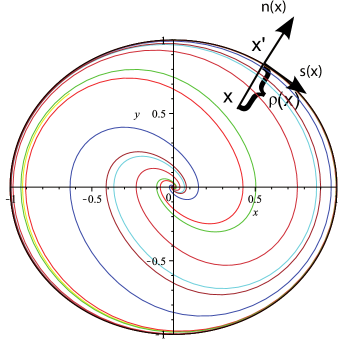
Figure 1: The field $\mbox{\boldmath$a$}(\mbox{\boldmath$x$})=[y,-x-y(1-x^{2}-y^{2})]^{T}$ has a stable focus at the origin and the boundary of the domain $D$ is a limit cycle.

The transformation is given by $\mbox{\boldmath$x$}=\mbox{\boldmath$x$}^{\prime}+\rho\nabla\rho(\mbox{\boldmath$x$}^{\prime}),$ where $\mbox{\boldmath$x$}^{\prime}$ is a function of $s$. The local representation of the field $\mbox{\boldmath$a$}(\mbox{\boldmath$x$})$ in the boundary strip is assumed

$$\mbox{\boldmath$a$}(\rho,s)=\left[a^{0}(s)\rho\nabla\rho+B(s)\nabla s\right][1+o(1)]\hskip 5.0pt\mbox{for}\ \rho\to 0,$$ (14)

that is, the tangential component of the field at $\partial D$ is

$$B(s)=\mbox{\boldmath$a$}(0,s)\cdot\nabla s=|\mbox{\boldmath$a$}(\mbox{\boldmath$x$}(s))|>0$$ (15)

and the normal derivative of the normal component is $a^{0}(s)\geq 0$ for all $0\leq s\leq S$. The decomposition (14) for the field $\mbox{\boldmath$a$}(\rho,s)$ in Figure 1 is given by $a^{0}(s)=2\sin^{2}s,\ B(s)=1$.

3.2 The WKB structure of the principal eigenfunction

3.2.1 The eikonal equation

We begin with the construction of the asymptotic approximation of the principal eigenfunction, now denoted $u(\mbox{\boldmath$y$})$. According to (Schuss, 2010, Section 10.2.6), it has the WKB structure

$$u(\mbox{\boldmath$y$})=K_{\displaystyle\varepsilon}(\mbox{\boldmath$y$})\exp\!\left\{-\frac{\psi(\mbox{\boldmath$y$})}{\varepsilon}\right\},$$ (16)

where the eikonal function $\psi(\mbox{\boldmath$y$})$ is solution of the Hamilton-Jacobi (eikonal) equation

$$\mbox{\boldmath$\sigma$}(\mbox{\boldmath$y$})\nabla\psi(\mbox{\boldmath$y$})\cdot\nabla\psi(\mbox{\boldmath$y$})+\mbox{\boldmath$a$}(\mbox{\boldmath$y$})\cdot\nabla\psi(\mbox{\boldmath$y$})=0,$$ (17)

which is obtained by substituting (16) in (3) and comparing to zero the leading term in the expansion of the resulting equation in powers of $\varepsilon$ (Matkowsky and Schuss, 1977), (Schuss, 1980), (Matkowsky and Schuss, 1982). An interpretation of the eikonal function $\psi(\mbox{\boldmath$y$})$ in terms of the calculus of variations is given in large deviations theory (Freidlin and Wentzell, 1984).

The solution $\psi(\mbox{\boldmath$x$})$ of the eikonal equation (17) near the origin (the focus) is given by

$$\psi(\mbox{\boldmath$x$})=\frac{1}{2}\mbox{\boldmath$x$}^{T}\mbox{\boldmath$Q$}\mbox{\boldmath$x$}+o(|\mbox{\boldmath$x$}|^{2})\hskip 5.0pt\mbox{for}\ \mbox{\boldmath$x$}\to\mbox{\boldmath$0$}$$ (18)

with $Q$ the solution of the Riccati equation

$$2\mbox{\boldmath$Q$}\mbox{\boldmath$\sigma$}(\mbox{\boldmath$0$})\mbox{\boldmath$Q$}+\mbox{\boldmath$Q$}\mbox{\boldmath$A$}+\mbox{\boldmath$A$}^{T}\mbox{\boldmath$Q$}=\mbox{\boldmath$0$}.$$ (19)

where $\psi(\mbox{\boldmath$x$})$ is the solution of the eikonal equation (17). The eikonal function $\psi(\mbox{\boldmath$x$})$ is constant on $\partial D$ with the local expansion

$$\psi(\rho,s)=\hat{\psi}+\frac{1}{2}\rho^{2}\phi(s)+o(\rho^{2})\hskip 5.0pt\mbox{for}\ \rho\to 0,$$ (20)

where $\phi(s)$ is the $S$-periodic solution of the Bernoulli equation

$$\sigma(s)\phi^{2}(s)+a^{0}(s)\phi(s)+\frac{1}{2}B(s)\phi^{\prime}(s)=0$$ (21)

and where $\sigma(s)=\mbox{\boldmath$\sigma$}(0,s)\nabla\rho(0,s)\cdot\nabla\rho(0,s).$ We may assume that for isotropic diffusion $\sigma(s)=1$. Thus, for the dynamics in Fig.1, the value of the constant $\hat{\psi}$ is calculated by integrating the characteristic equations for the eikonal equation (17) (Schuss, 2010).

To prove (20), we note that $\psi(\mbox{\boldmath$y$})$ is constant on the boundary, because in local coordinates on $\partial D$ (17) can be written as

$$[\nabla\psi(0,s)]^{T}\mbox{\boldmath$\sigma$}(0,s)\nabla\psi(0,s)+B(s)\frac{\partial\psi(0,s)}{\partial s}=0.$$ (22)

To be well defined on the boundary, the function $\psi(0,s)$ must be periodic in $s$ with period $S$. However, (22) implies that the derivative $\partial\psi(0,s)/\partial s$ does not change sign, because $B(s)>0$ and the matrix $\mbox{\boldmath$\sigma$}(0,s)$ is positive definite. Thus we must have

$$\psi(0,s)=\mbox{const.}=\hat{\psi},\quad\nabla\psi(0,s)=0\hskip 5.0pt\mbox{for all}\ 0\leq s\leq S.$$ (23)

It follows that near $\partial D$ the following expansion holds,

$$\psi(\rho,s)=\hat{\psi}+\frac{1}{2}\rho^{2}\frac{\partial^{2}\psi(0,s)}{\partial\rho^{2}}+o\left(\rho^{2}\right)\hskip 5.0pt\mbox{as}\ \rho\to 0.$$

Setting $\phi(s)=\partial^{2}\psi(0,s)/\partial\rho^{2}$ and using (14) and (20) in (17), we see that $\phi(s)$ must be the $S$-periodic solution of the Bernoulli equation (21) and $\sigma(s)=\mbox{\boldmath$\sigma$}(0,s)\nabla\rho(0,s)\cdot\nabla\rho(0,s)$. Writing $\xi_{0}(s)=\sqrt{-\phi(s)}$ in (21), we see that $\xi_{0}(s)$ is the $S$-periodic solution of the Bernoulli equation

$$B(s)\xi_{0}^{\prime}(s)+a^{0}(s)\xi_{0}(s)-\sigma(s)\xi_{0}^{3}(s)=0.$$ (24)

These function are discussed further in section 3.3.

3.2.2 The transport equation

The function $K_{\displaystyle\varepsilon}(\mbox{\boldmath$y$})$ is a regular function of $\varepsilon$ for $\mbox{\boldmath$y$}\in D$, but has to develop a boundary layer to satisfy the homogenous Dirichlet boundary condition

$$K_{\displaystyle\varepsilon}(\mbox{\boldmath$y$})=0\hskip 5.0pt\mbox{for}\ \mbox{\boldmath$y$}\in\partial D.$$ (25)

Therefore $K_{\displaystyle\varepsilon}(\mbox{\boldmath$y$})$ is further decomposed into the product

$$K_{\displaystyle\varepsilon}(\mbox{\boldmath$y$})=\left[K_{0}(\mbox{\boldmath$y$})+\varepsilon K_{1}(\mbox{\boldmath$y$})+\cdots\right]q_{\displaystyle\varepsilon}(\mbox{\boldmath$y$}),$$ (26)

where $K_{0}(\mbox{\boldmath$y$}),\,K_{1}(\mbox{\boldmath$y$}),\,\ldots$ are regular functions in $D$ and on its boundary and are independent of $\varepsilon$, and $q_{\displaystyle\varepsilon}(\mbox{\boldmath$y$})$ is a boundary layer function. As in the case of the eikonal equation $\psi(\mbox{\boldmath$y$})$, the functions $K_{j}(\mbox{\boldmath$y$})\ (j=0,1,\dots)$ are solutions of first-order linear transport equations derived by substituting (16) in (3), expanding the resulting equation in powers of $\varepsilon$, and equating to zero their coefficients (Matkowsky and Schuss, 1977), (Schuss, 1980). These functions cannot satisfy the boundary condition (25), because they are solutions of first-order equations. Thus $K_{0}(\mbox{\boldmath$y$})$ has to be found by integrating a transport equation along characteristics. Consequently, a boundary layer function $q_{\varepsilon}(\mbox{\boldmath$y$})$ is needed to make (26) satisfy the homogeneous Dirichlet boundary condition.

The boundary layer function $q_{\displaystyle\varepsilon}(\mbox{\boldmath$y$})$ has to satisfy the boundary condition

$$q_{\varepsilon}(\mbox{\boldmath$y$})=0\hskip 5.0pt\mbox{for}\ \mbox{\boldmath$y$}\in\partial D,$$ (27)

the matching condition

$$\lim_{\varepsilon\to 0}q_{\varepsilon}(\mbox{\boldmath$y$})= \,1\hskip 5.0pt\mbox{for all}\ \mbox{\boldmath$y$}\in D,$$ (28)

and the smoothness condition

$$\lim_{\varepsilon\to 0}\frac{\partial^{i}q_{\varepsilon}(\mbox{\boldmath$y$})}{\partial(y^{j})^{i}}=0,\hskip 5.0pt\mbox{for all}\ \mbox{\boldmath$y$}\in D,\ i\geq 1,\,1\leq j\leq 2.$$ (29)

First, we derive the transport equation for the leading term $K_{0}(\mbox{\boldmath$y$})$. The function $K_{\displaystyle\varepsilon}(\mbox{\boldmath$y$})$, which satisfies the transport equation

$$\,\varepsilon\sum_{i,j=1}^{2}\frac{\partial^{2}\sigma^{i,j}(\mbox{\boldmath$y$})K_{\displaystyle\varepsilon}(\mbox{\boldmath$y$})}{\partial y^{i}\partial y^{j}}$$

$$\,-\sum_{i=1}^{2}\left[2\sum_{j=1}^{d}\sigma^{i,j}(\mbox{\boldmath$y$})\frac{\partial\psi(\mbox{\boldmath$y$})}{\partial y^{j}}+a^{i}(\mbox{\boldmath$y$})\right]\frac{\partial K_{\displaystyle\varepsilon}(\mbox{\boldmath$y$})}{\partial y^{i}}$$

$$\,-\sum_{i=1}^{2}\left\{\frac{\partial a^{i}(\mbox{\boldmath$y$})}{\partial y^{i}}+\sum_{j=1}^{2}\left[\sigma^{i,j}(\mbox{\boldmath$y$})\frac{\partial^{2}\psi(\mbox{\boldmath$y$})}{\partial y^{i}\partial y^{j}}+2\frac{\partial\sigma^{i,j}(\mbox{\boldmath$y$})}{\partial y^{j}}\frac{\partial\psi(\mbox{\boldmath$y$})}{\partial y^{j}}\right]\right\}K_{\displaystyle\varepsilon}(\mbox{\boldmath$y$})=0,$$ (30)

cannot have an internal layer at the global attractor point $\mathrm{𝟎}$ in $D$, because stretching $\mbox{\boldmath$y$}=\sqrt{\varepsilon}\mbox{\boldmath$\xi$}$ and taking the limit $\varepsilon\to 0$ converts the transport equation (30) to

$$\,\sum_{i,j=1}^{d}\frac{\partial^{2}\sigma^{i,j}(\mbox{\boldmath$0$})K_{0}(\mbox{\boldmath$\xi$})}{\partial\xi^{i}\partial\xi^{j}}-(2\mbox{\boldmath$A$}\mbox{\boldmath$Q$}+\mbox{\boldmath$A$})\mbox{\boldmath$\xi$}\cdot\nabla_{\mbox{\boldmath$\xi$}}K_{0}(\mbox{\boldmath$\xi$})$$

$$\,-\mbox{tr}\left(\mbox{\boldmath$A$}+\mbox{\boldmath$\sigma$}(\mbox{\boldmath$0$})\mbox{\boldmath$Q$}\right)K_{0}(\mbox{\boldmath$\xi$})=0,$$

whose bounded solution is $K_{0}(\mbox{\boldmath$y$})=const,$ because $\mbox{tr}\left(\mbox{\boldmath$A$}+\mbox{\boldmath$\sigma$}(\mbox{\boldmath$0$})\mbox{\boldmath$Q$}\right)=0.$ The last equality follows from the Riccati equation (19) (left multiply by $\mbox{\boldmath$Q$}^{-1}$ and take the trace).

In view of eqs. (26)–(29), we obtain in the limit $\varepsilon\to 0$ the transport equation

$$\,\sum_{i=1}^{d}\left[2\sum_{j=1}^{d}\sigma^{i,j}(\mbox{\boldmath$y$})\frac{\partial\psi(\mbox{\boldmath$y$})}{\partial y^{j}}+a^{i}(\mbox{\boldmath$y$})\right]\frac{\partial{K_{0}(\mbox{\boldmath$y$})}}{\partial y^{i}}$$ (31)

$$= \,-\sum_{i=1}^{d}\left\{\frac{a^{i}(\mbox{\boldmath$y$})}{\partial y^{i}}+\sum_{j=1}^{d}\left[\sigma^{i,j}(\mbox{\boldmath$y$})\frac{\partial^{2}\psi(\mbox{\boldmath$y$})}{\partial y^{i}\partial y^{j}}+2\frac{\partial\sigma^{i,j}(\mbox{\boldmath$y$})}{\partial y^{j}}\frac{\partial\psi(\mbox{\boldmath$y$})}{\partial y^{j}}\right]\right\}{K_{0}(\mbox{\boldmath$y$})}.$$

Because the characteristics diverge, the initial value on each characteristic of the eikonal equation (17) is given at $\mbox{\boldmath$y$}=\mbox{\boldmath$0$}$ as $K_{0}(\mbox{\boldmath$0$})=const.$ (e.g., $const.=1$).

Note that using (14) and (17), the field in the transport equation (30) can be written in local coordinates near the boundary as

$$2\mbox{\boldmath$\sigma$}(\mbox{\boldmath$y$})\nabla\psi(\mbox{\boldmath$y$})+\mbox{\boldmath$a$}(\mbox{\boldmath$y$})= \,2\mbox{\boldmath$\sigma$}(0,s)\nabla\psi(0,s)+\mbox{\boldmath$a$}(0,s)+o(\rho)$$

$$= \,\rho\left[2\phi(s)\mbox{\boldmath$\sigma$}(0,s)\nabla\rho(0,s)+a^{0}(s)\nabla\rho(0,s)\right]+o(\rho)$$ (32)

and the transport equation for $K_{0}(\mbox{\boldmath$y$})$ can be written on $\partial D$ as the linear equation (which corrects eq.(10.125) in (Schuss, 2010))

$$B(s)\frac{dK_{0}(0,s)}{ds}+[a^{0}(s)+\sigma(s)\phi(s)+B^{\prime}(s)]K_{0}(0,s)=0.$$ (33)

Using the relations (61) below, we obtain the solution

$$K_{0}(0,s)=K_{0}\frac{\sqrt{-\phi(s)}}{B(s)},$$ (34)

where $K_{0}=const.$ (e.g., $K_{0}=1$).

3.2.3 The boundary layer equation for $q_{\displaystyle\varepsilon}(\mbox{\boldmath$x$})$

To derive the boundary layer equation, we introduce the stretched variable $\zeta=\rho/\sqrt{\varepsilon}$ and define $q_{\displaystyle\varepsilon}(\mbox{\boldmath$x$})=Q(\zeta,s,\varepsilon)$. Expanding all functions in (16) in powers of $\varepsilon$ and

$$Q(\zeta,s,\varepsilon)\sim Q^{0}(\zeta,s)+\sqrt{\varepsilon}Q^{1}(\zeta,s)+\cdots,$$ (35)

and using (32), we obtain the boundary layer equation

$$\sigma(s)\frac{\partial^{2}Q^{0}(\zeta,s)}{\partial\zeta^{2}}-\zeta\left[a^{0}(s)+2\sigma(s)\phi(s)\right]\frac{\partial Q^{0}(\zeta,s)}{\partial\zeta}-B(s)\frac{\partial Q^{0}(\zeta,s)}{\partial s}=0.$$ (36)

The boundary and matching conditions (27), (28) imply that

$$Q^{0}(0,s)=0,\quad\lim_{\zeta\to-\infty}Q^{0}(\zeta,s)=1.$$ (37)

To solve (36), (37), we set $\eta=\xi(s)\zeta$, $Q^{0}(\zeta,s)=\tilde{Q}^{0}(\eta,s)$, and rewrite (36) as

$$\sigma(s)\xi^{2}(s)\frac{\partial^{2}\tilde{Q}^{0}(\eta,s)}{\partial\eta^{2}}- \eta\left[a^{0}(s)+2\sigma(s)\phi(s)+\frac{B(s)\xi^{\prime}(s)}{\xi(s)}\right]\frac{\partial\tilde{Q}^{0}(\eta,s)}{\partial\eta}$$

$$- B(s)\frac{\partial\tilde{Q}^{0}(\eta,s)}{\partial s}=0.$$ (38)

Choosing $\xi(s)$ to be the $S$-periodic solution of the Bernoulli equation (21) the boundary value and matching problem (36), (37) becomes

$$\frac{\partial^{2}\tilde{Q}^{0}(\eta,s)}{\partial\eta^{2}}+\eta\frac{\partial\tilde{Q}^{0}(\eta,s)}{\partial\eta}-\frac{B(s)}{\sigma(s)\xi^{2}(s)}\frac{\partial\tilde{Q}^{0}(\eta,s)}{\partial s} \,=0,$$ (39)

$$\tilde{Q}^{0}(0,s)=0,\quad\lim_{\eta\to-\infty}\tilde{Q}^{0}(\eta,s) \,=1,$$ (40)

which has the $s$-independent solution

$$\tilde{Q}^{0}(\eta,s)=-\sqrt{\frac{2}{\pi}}\int\limits_{0}^{\eta}e^{-z^{2}/2}\,dz,$$ (41)

that is,

$$Q^{0}(\zeta,s)=-\sqrt{\frac{2}{\pi}}\int\limits_{0}^{\xi(s)\zeta}e^{-z^{2}/2}\,dz.$$ (42)

The uniform expansion of the first eigenfunction is constructed by putting together (16), (26), (35), and (42) to obtain that

$$u_{0}(\mbox{\boldmath$y$})=\exp\left\{-\frac{\psi(\mbox{\boldmath$y$})}{\varepsilon}\right\}\left[K_{0}(\mbox{\boldmath$y$})+O(\sqrt{\varepsilon})\right]\sqrt{\frac{2}{\pi}}\int\limits_{0}^{\displaystyle\frac{-\rho(\mbox{\boldmath$y$})\xi(s(\mbox{\boldmath$y$}))}{\sqrt{\varepsilon}}}e^{-z^{2}/2}\,dz,$$ (43)

where $O(\sqrt{\varepsilon})$ is uniform in $\mbox{\boldmath$y$}\in\bar{D}$.

Because $\eta=\xi(s)\zeta=\xi(s)\rho/\sqrt{\varepsilon}$, equations (20) and (61) near the boundary give

$$\psi(\rho,s)=\hat{\psi}-\frac{\rho^{2}\xi^{2}(s)}{2}+o(\rho^{2}),$$ (44)

so the eigenfunction (43) near the limit cycle has the form

$$u_{0}(\mbox{\boldmath$y$})\sim{\exp\left\{-\frac{\hat{\psi}}{\varepsilon}\right\}}\exp\left\{-\frac{\eta^{2}}{2}\right\}\left[K_{0}(\mbox{\boldmath$y$})+O(\sqrt{\varepsilon})\right]\sqrt{\frac{2}{\pi}}\int\limits_{0}^{-\eta}e^{-z^{2}/2}\,dz.$$ (45)

The function $u_{0}(\mbox{\boldmath$y$})$ is defined up to a multiplicative constant.

The eigenfunction expansion (9) and the expansion (43) of the principal eigenfunctions of the operator and its adjoint, respectively, give the probability flux density

$$\mbox{\boldmath$J$}\cdot\mbox{\boldmath$\nu$}|_{\partial D}(s,t)\sim e^{-\lambda_{0}t}\sqrt{\frac{2\varepsilon}{\pi}}K_{0}(0,s)\xi(s)\sigma(s)e^{-\hat{\psi}/\varepsilon}+\ldots,$$ (46)

hence, for $\mbox{\boldmath$y$}\in\partial D$, which corresponds to $\rho=0$ and arclength $s$,

$$\,\Pr\{\mbox{\boldmath$x$}(\tau)=\mbox{\boldmath$y$},\tau=t\,|\,\mbox{\boldmath$x$}(0)=\mbox{\boldmath$x$}\}$$

$$= \,\frac{K_{0}(0,s)\xi(s)\sigma(s)+e^{(\lambda_{0}-\lambda_{n,m})t}u_{n,m}(\mbox{\boldmath$y$})v_{n,m}(\mbox{\boldmath$x$})+\ldots}{\displaystyle\int_{0}^{S}K_{0}(0,s)\xi(s)\sigma(s)\,ds+e^{(\lambda_{0}-\lambda_{n,m})t}u_{n,m}(\mbox{\boldmath$y$})v_{n,m}(\mbox{\boldmath$x$})+\ldots\,\displaystyle}.$$ (47)

Using (45) at $\eta=0$ and (34), we recover in the limit $t\to\infty$ the exit density at $\mbox{\boldmath$y$}=(0,s)$ as (Schuss, 2010)

$$\Pr\{\mbox{\boldmath$x$}(\tau)=\mbox{\boldmath$y$}\,|\,\mbox{\boldmath$x$}\}\sim\frac{\displaystyle\frac{\xi^{2}(s)\sigma(s)}{B(s)}}{\displaystyle{\int_{0}^{S}}\displaystyle\frac{\xi^{2}(s)\sigma(s)}{B(s)}\,ds},$$ (48)

which to leading order is independent of $x$ outside a boundary layer of width $\sqrt{\varepsilon}$.

3.2.4 The first eigenfunction of the adjoint problem

The first eigenfunction $v_{0}(\mbox{\boldmath$x$})$ of the backward operator $L^{*}_{\mbox{\boldmath$x$}}$ does not have the WKB structure (16), but rather converges to a constant as $\varepsilon\to 0$, at every $\mbox{\boldmath$x$}\in D$ outside the boundary layer. Thus it is merely the boundary layer $q_{\displaystyle\varepsilon}(\mbox{\boldmath$y$})$. Expanding as in section 3.2.3, we obtain the boundary value and matching problem

$$\sigma(s)\frac{\partial^{2}Q^{0}(\zeta,s)}{\partial\zeta^{2}}+\zeta a^{0}(s)\frac{\partial Q^{0}(\zeta,s)}{\partial\zeta}+B(s)\frac{\partial Q^{0}(\zeta,s)}{\partial s}=0$$ (49)

$$Q^{0}(0,s)=0,\quad\lim_{\zeta\to-\infty}Q^{0}(\zeta,s)=1.$$ (50)

The scaling $\eta=\xi_{0}(s)\eta$, with $\xi_{0}(s)$ the solution of (24), converts (49), (50) to

$$\frac{\partial^{2}\tilde{Q}^{0}(\eta,s)}{\partial\eta^{2}}+\eta\frac{\partial\tilde{Q}^{0}(\eta,s)}{\partial\eta}+\frac{B(s)}{\sigma(s)\xi^{2}(s)}\frac{\partial\tilde{Q}^{0}(\eta,s)}{\partial s} \,=0,$$ (51)

$$\tilde{Q}^{0}(0,s)=0,\quad\lim_{\eta\to-\infty}\tilde{Q}^{0}(\eta,s) \,=1,$$ (52)

where $\tilde{Q}^{0}(\eta,s)=Q^{0}(\zeta,s)$. Using the solution of the Bernoulli equation (61), we obtain the $s$-independent solution (41) and hence (42), which is the uniform approximation to $v_{0}(\mbox{\boldmath$y$})$. We conclude that

$$v_{0}(\mbox{\boldmath$y$})={C_{\varepsilon}}\mbox{erf}\left(\frac{\rho(\mbox{\boldmath$y$})\xi(s(\mbox{\boldmath$y$}))}{\sqrt{\varepsilon}}\right),$$ (53)

where $C_{\varepsilon}$ depends on the normalization. Thus

$$u_{0}(\mbox{\boldmath$y$})\sim\exp\left\{-\frac{\psi(\mbox{\boldmath$y$})}{\varepsilon}\right\}\left[K_{0}(\mbox{\boldmath$y$})+O(\sqrt{\varepsilon})\right]v_{0}(\mbox{\boldmath$y$}),$$ (54)

which in the boundary layer coordinates has the form

$$u_{0}(\mbox{\boldmath$y$})\sim\exp\left\{-\frac{\eta^{2}}{2}\right\}\left[K_{0}(\mbox{\boldmath$y$})+O(\sqrt{\varepsilon})\right]v_{0}(\mbox{\boldmath$y$}).$$ (55)

3.3 The principal eigenvalue $\lambda_{0}$ and the mean first passage time

The asymptotic expansion of the mean first passage time $\bar{\tau}(\mbox{\boldmath$x$})$ from $\mbox{\boldmath$x$}\in D$ to the boundary is the solution of the Pontryagin-Andronov-Vitt boundary value problem (Matkowsky and Schuss, 1982), (Schuss, 2010, Section 10.2.8)

$$L^{*}\bar{\tau}(\mbox{\boldmath$x$})= \,-1\hskip 5.0pt\mbox{for}\ \mbox{\boldmath$x$}\in D$$ (56)

$$\bar{\tau}(\mbox{\boldmath$x$})= \,0\hskip 5.0pt\mbox{for}\ \mbox{\boldmath$x$}\in\partial D.$$ (57)

It is known to be independent of $x$ outside the boundary layer in the sense that

$$\lim\limits_{\varepsilon\to 0}\frac{\bar{\tau}(\mbox{\boldmath$x$})}{\bar{\tau}(\mbox{\boldmath$0$})}=1,$$

where

$$\bar{\tau}(\mbox{\boldmath$0$})\sim\frac{\pi^{3/2}\sqrt{2\varepsilon\,\mbox{det}\mbox{\boldmath$Q$}}}{\displaystyle\int_{0}^{S}K_{0}(s)\xi(s)\,ds}\exp\left\{\frac{\hat{\psi}}{\varepsilon}\right\}.$$ (58)

The function $K_{0}(s)$, given by,

$$K_{0}(s)=\frac{1}{B(s)}\exp\left\{-\int_{0}^{s}\left[\frac{a_{0}(s^{\prime})-\xi^{2}(s^{\prime})}{B(s^{\prime})}\,ds^{\prime}\right]\right\},$$ (59)

where $\xi(s)$ is the $S$-periodic solution of the Bernoulli equation

$$\sigma(s)\xi^{3}(s)+[a^{0}(s)+2\sigma(s)\phi(s)]\xi(s)+B(s)\xi^{\prime}(s)=0,$$ (60)

is defined up to a multiplicative constant that can be chosen to be 1. The solutions of the three Bernoulli equations $\phi(s)$ of (21), $\xi(s)$ of (60), and $\xi_{0}(s)$ of (24) are related to each other as follows (see (Schuss, 2010, Section 10.2.6) and Section 10.2.8),

$$\xi_{0}(s)=\sqrt{-\phi(s)}=\xi(s).$$ (61)

The mean first passage time from $\mbox{\boldmath$x$}\in D$ to the boundary is also given by (Schuss, 2010)

$$\bar{\tau}(\mbox{\boldmath$x$}) = \int\limits_{0}^{\infty}t\Pr\{\tau=t\,|\,\mbox{\boldmath$x$}\}dt=\int\limits_{0}^{\infty}\Pr\{\tau>t\,|\,\mbox{\boldmath$x$}\}=\int\limits_{0}^{\infty}\int_{D}p_{\varepsilon}(\mbox{\boldmath$y$},t\,|\,\mbox{\boldmath$x$})dtd\mbox{\boldmath$y$}$$ (62)

$$= \frac{1}{\lambda_{0}}v_{0}(\mbox{\boldmath$x$})+\sum_{n,m}\frac{\bar{v}_{n,m}(\mbox{\boldmath$x$})}{\lambda_{n,m}}\int\limits_{D}u_{n,m}(\mbox{\boldmath$y$})\,d\mbox{\boldmath$y$}.$$

If $x$ is outside the boundary layer, then $v_{0}(\mbox{\boldmath$x$})\sim 1$, as shown above, and $\int_{D}u_{n,m}(\mbox{\boldmath$y$})\,d\mbox{\boldmath$y$}\sim 0$ by bi-orthogonality. Therefore

$$\bar{\tau}(\mbox{\boldmath$x$})=\frac{1}{\lambda_{0}}v_{0}(\mbox{\boldmath$x$})(1+o(1))\hskip 5.0pt\mbox{for}\ \varepsilon\ll 1.$$ (63)

The principal eigenvalue $\lambda_{0}$ introduced in (2) is thus given more precisely by the asymptotic relation

$$\lambda_{0}\sim\frac{1}{\bar{\tau}(\mbox{\boldmath$0$})}\hskip 5.0pt\mbox{for}\ \varepsilon\ll 1$$ (64)

and in view of (58), $\lambda_{0}$ decreases exponentially fast as $\varepsilon\to 0$.

4 Higher order eigenvalues

The asymptotic expansion of higher-order eigenfunctions is constructed by the method used above to derive that of the principal eigenfunctions. First, we consider higher-order eigenfunctions of the adjoint problem, which leads to the boundary layer equation and matching conditions

$$\frac{\partial^{2}\tilde{Q}^{0}(\eta,s)}{\partial\eta^{2}}+\eta\frac{\partial\tilde{Q}^{0}(\eta,s)}{\partial\eta}+\frac{B(s)}{\sigma(s)\xi^{2}(s)}\frac{\partial\tilde{Q}^{0}(\eta,s)}{\partial s} \,=-\frac{\lambda}{\sigma(s)\xi^{2}(s)}\tilde{Q}^{0}(\eta,s),$$ (65)

$$\tilde{Q}^{0}(0,s)=0,\quad\lim_{\eta\to-\infty}\tilde{Q}^{0}(\eta,s) \,=0.$$ (66)

Separating $\tilde{Q}^{0}(\eta,s)=R(\eta)T(s)$, we obtain for the even function $R(\eta)$ the eigenvalue problem

$$R^{\prime\prime}(\eta)+\eta R^{\prime}(\eta)+\mu R(\eta)=0,\quad R(0)=0,\quad\lim_{\eta\to-\infty}R(\eta)=0,$$ (67)

where $\mu$ is the separation constant. The large $\eta$ asymptotics of $R(\eta)$ is $R(\eta)\sim\exp\{-\eta^{2}/2\}$, so the substitution $R(\eta)=\exp\{-\eta^{2}/4\}W(\eta)$ converts (67) to the parabolic cylinder function eigenvalue problem

$$W^{\prime\prime}(\eta)+\left(\mu-\frac{1}{2}-\frac{\eta^{2}}{4}\right)W(\eta)=0,\quad W(0)=0,\quad\lim_{\eta\to-\infty}W(\eta)=0.$$ (68)

The eigenvalues of the problem (68) are $\mu_{n}=2n,\ (n=1,2,\ldots)$ with the eigenfunctions

$$W_{2n+1}(\eta)=\exp\left\{-\frac{\eta^{2}}{4}\right\}H_{2n+1}\left(\frac{\eta}{\sqrt{2}}\right),$$

where $H_{2n+1}(x)$ are the Hermite polynomials of odd orders (Abramowitz and Stegun, 1972). Thus the radial eigenfunctions are

$$R_{n}(\eta)=\exp\left\{-\frac{\eta^{2}}{4}\right\}W_{2n+1}(\eta)=\exp\left\{-\frac{\eta^{2}}{2}\right\}H_{2n+1}\left(\frac{\eta}{\sqrt{2}}\right).$$ (69)

The associated function $T(s)$ (normalized to one) is the $S$-periodic solution of

$$-\mu_{n}T(s)+\frac{B(s)}{\sigma(s)\xi^{2}(s)}\frac{\partial T(s)}{\partial s} \,=-\frac{\lambda}{\sigma(s)\xi^{2}(s)}T(s),$$ (70)

given by

$$T_{n}(s)=\exp\left\{-\lambda\int_{0}^{s}\frac{ds^{\prime}}{B(s^{\prime})}+2n\int_{0}^{s}\frac{\sigma(s^{\prime})\xi^{2}(s^{\prime})}{B(s^{\prime})}\,ds^{\prime}\right\}.$$ (71)

We introduce therefore the period and angular frequency of rotation of the drift about the boundary which are, respectively,

$${\cal T}=\int_{0}^{S}\frac{ds^{\prime}}{B(s^{\prime})},\quad\omega=\frac{2\pi}{\cal T}.$$

Thus $S$-periodicity implies the relation

$$-\lambda\int_{0}^{S}\frac{ds}{B(s)}+2n\int_{0}^{S}\frac{\sigma(s)\xi^{2}(s)}{B(s)}\,ds=2\pi mi$$ (72)

for $m=\pm 1,\pm 2,\ldots\,.$ It follows that for $n=1,\ldots$ the eigenvalues are

$$\lambda_{m,n}=\left[\frac{n}{\pi}\int_{0}^{S}\frac{\sigma(s)\xi^{2}(s)}{B(s)}\,ds+mi\right]\omega$$ (73)

and the rotational eigenfunctions are

$$T_{m,n}(s)=\exp\left\{-\lambda_{m,n}\int_{0}^{s}\frac{ds^{\prime}}{B(s^{\prime})}+2n\int_{0}^{s}\frac{\sigma(s^{\prime})\xi^{2}(s^{\prime})}{B(s^{\prime})}\,ds^{\prime}\right\}.$$ (74)

The eigenfunctions $\tilde{Q}_{m,n}(\eta,s)=R_{n}(\eta)T_{m,n}(s)$ are given by

$$\tilde{Q}_{m,n}(\eta,s)=\exp\left\{-\frac{\eta^{2}}{2}\right\}H_{2n+1}\left(\frac{\eta}{\sqrt{2}}\right)\exp\left\{-mi\omega\int_{0}^{s}\frac{ds^{\prime}}{B(s^{\prime})}+2n\int_{0}^{s}\frac{\sigma(s^{\prime})\xi^{2}(s^{\prime})}{B(s^{\prime})}\,ds^{\prime}\right\}.$$ (75)

Thus the expressions (64), (58), and (73) define the spectrum as

$$Sp(L)=\left\{\lambda_{0}(1+O(\varepsilon)),\bigcup_{n\geq 0,m=\pm 1,\pm 2,\ldots}\lambda_{m,n}(1+O(\varepsilon))\right\}.$$ (76)

As in (54), the forward eigenfunctions $u_{n,m}(\mbox{\boldmath$y$})$ are related to the backward eigenfunctions $v_{n,m}(\mbox{\boldmath$y$})=\tilde{Q}_{m,n}(\eta,s)$ by

$$u_{n,m}(\mbox{\boldmath$y$})\sim\exp\left\{-\frac{\psi(\mbox{\boldmath$y$})}{\varepsilon}\right\}\left[K_{0}(\mbox{\boldmath$y$})+O(\sqrt{\varepsilon})\right]\bar{v}_{n,m}(\mbox{\boldmath$y$}),$$ (77)

where in the initial variable

$$v_{n,m}(\mbox{\boldmath$y$}) = \displaystyle\exp\left\{-\frac{[\rho(\mbox{\boldmath$y$})\xi(s(\mbox{\boldmath$y$}))]^{2}}{2\varepsilon}\right\}H_{2n+1}\left(\frac{\rho(\mbox{\boldmath$y$})\xi(s(\mbox{\boldmath$y$}))}{\sqrt{2\varepsilon}}\right)$$

$$\times \exp\left\{-mi\omega\int\limits_{0}^{s(\mbox{\boldmath$y$})}\frac{ds^{\prime}}{B(s^{\prime})}+2n\int\limits_{0}^{s(\mbox{\boldmath$y$})}\frac{\sigma(s^{\prime})\xi^{2}(s^{\prime})}{B(s^{\prime})}\,ds^{\prime}\right\}.$$

which in the boundary layer coordinates has the form

$$u_{n,m}(\mbox{\boldmath$y$})\sim\exp\left\{-\frac{\eta^{2}}{2}\right\}\left[K_{0}(\mbox{\boldmath$y$})+O(\sqrt{\varepsilon})\right]\bar{v}_{n,m}(\mbox{\boldmath$y$}).$$ (78)

With the proper normalization the eigenfunctions $\{u_{n,m}(\mbox{\boldmath$y$})\}$ and $\{v_{n,m}(\mbox{\boldmath$y$})\}$ form a bi-orthonormal system.

5 Applications

The asymptotic theory of section 4 applies to a well-known model in neurophysiology, proposed in (Holcman and Tsodyks, 2006). In the absence of sensory stimuli the cerebral cortex is continuously active. An example of this spontaneous activity is the phenomenon of voltage transitions between two distinct levels, called Up and Down states, observed simultaneously when recoding from many neurons (Anderson et al., 2000), (Cossart et al., 2003). The mathematical model proposed in (Holcman and Tsodyks, 2006) for cortical dynamics that exhibits spontaneous transitions between Up- and Down- states is given by the stochastic dynamics

$$\dot{x} = \frac{1-x}{t_{r}}-Ux(y-T)H(y-T),$$

$$\dot{y} = -\frac{y}{\tau}+\frac{xUw_{T}}{\tau}(y-T)H(y-T)+\frac{\sigma}{\sqrt{\tau}}\,\dot{w},$$

where $x$ is a dimensionless synaptic depression parameter, $y$ is the membrane voltage, $U$ and $t_{r}$ are utilization parameter and recovery time constant, respectively, $w_{T}$ is synaptic strength, $\tau$ is a voltage time scale, $\sigma$ is noise amplitude, $H(\cdot)$ is the Heaviside unit step function, and $\dot{w}$ is standard Gaussian white noise. The model (LABEL:HTmodel) predicts that in a certain range of parameters the noiseless dynamics (when $\sigma=0$) has two basins of attractions: one around a focus, which corresponds to an Up-state, and the second one is that of a stable equilibrium state, which corresponds to a Down-state. The basins of attraction are separated by an unstable limit cycle.

Figure 2A shows trajectories of (LABEL:HTmodel) that rotate several times around the focus before exiting the domain of attraction of the focus. Figure 2B shows the histogram of exit times oscillates with multiple peaks, as predicted by the theory presented in section 4 above. The approximation of the histogram of exit times (13) by the sum of the first two exponentials,

$$f(t)=A\exp(-\lambda_{0}t)+B\exp(-\lambda_{1}t)\cos(\omega t+\phi),$$ (80)

where $\lambda_{0}=\bar{\tau}^{-1}=1/2.46$ (computed empirically), $\lambda_{1}=2.5$ and the frequency is that of the focus (the imaginary part of the Jacobian at the focus) $\omega=10.4$. The other parameters are $A=470$, $B=600$, and $\phi=1.4$ (obtained by a numerical fit). The approximation (80) captures the first three oscillations that are smeared out in the exponentially decaying tail. The construction of the short-time histogram requires the entire series expansion in (13).

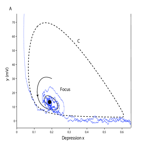
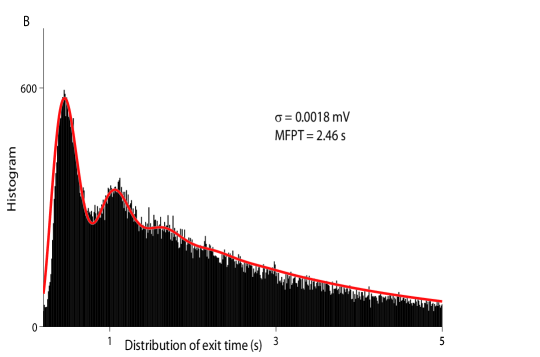
Figure 2: The phase-plane dynamics of (LABEL:HTmodel), restricted to the Up-state. A: The unstable limit cycle is C (dashed line) and simulated trajectories (blue). The parameters are $\tau=0.05\,sec,t_{r}=0.8\,sec,U=0.5,w_{T}=12.6\,mV/Hz,T=2.0\,mV$. B: Histogram of exit times and its approximation by the first two terms of the expansion (13) (marked red).

As indicated in section 4, the oscillation in the pdf of exit times is a manifestation of the complex eigenvalues of the non-self adjoint Dirichlet problem for the corresponding Fokker-Planck operator inside the limit cycle.

6 Summary and discussion

This paper explains the oscillatory decay of the survival probability of the stochastic dynamics (1) that is activated over the boundary of the domain of attraction $D$ of the stable focus of the drift $\mbox{\boldmath$a$}(\mbox{\boldmath$x$})$ by the small noise $\sqrt{2\varepsilon}\,\mbox{\boldmath$b$}(\mbox{\boldmath$x$}_{\varepsilon}(t))\,\dot{}\mbox{\boldmath$w$}(t)$. The boundary $\partial D$ of the domain is an unstable limit cycle of $\mbox{\boldmath$a$}(\mbox{\boldmath$x$})$. It is shown that the oscillations are not due a mysterious synchronization, but rather to complex eigenvalues of the Dirichlet problem for the Fokker-Planck operator in $D$. These are evaluated by a singular perturbation expansion of the spectrum of the non-self adjoint operator. The exact formula for the eigenvalues comes from the local expansion of the boundary layer in the neighborhood of the limit cycle. The expansion of the eigenvalues identifies for the first time the full and explicit spectrum of a non-self adjoint elliptic boundary value problem.

Oscillatory decay is manifested experimentally in the appearance of Up and Down states in the spontaneous activity of the cerebral cortex and in the simulations of its mathematical models (Holcman and Tsodyks, 2006). The oscillations are due to the competition between the driving noise and the underlying dynamical system.

References

- Anderson et al. (2000) Anderson, J., I. Lampl, I. Reichova, M. Carandini, D. Ferster (2000), ”Stimulus dependence of two-state fluctuations of membrane potential in cat visual cortex”. Nat. Neurosci. 3(6), pp.617–621.
- Abramowitz and Stegun (1972) Abramowitz, M. and I. Stegun (1972), Handbook of Mathematical Functions with Formulas, Graphs, and Mathematical Tables, Dover Publications, NY.
- Chavel (1984) Chavel, I. (1984), Eigenvalues in Riemannian geometry, Pure and Applied Mathematics, vol.115. Academic Press, Orlando, FL.
- Cossart et al. (2003) Cossart, R., D. Aronov, R. Yuste (2003), ”Attractor dynamics of network UP states in the neocortex,” Nature 15;423 (6937), pp.283–288.
- Davies (2002) Davies, E.B. (2002), ”Non-Self-Adjoint Differential Operators,” Bull. London Math. Soc. 34, pp.513–532.
- Devinatz and Friedman (1977) Devinatz, A. and A. Friedman (1977), ”The asymptotic behavior of the principal eigenvalue of singularly perturbed degenerate elliptic operators,” Illinois J. Math. 21, (4), pp.852–870.
- Freidlin and Wentzell (1984) Freidlin, M.I. and A.D. Wentzell (1984), Random Perturbations of Dynamical Systems, Grundlehren der mathematischen Wissenschaften (Book 260), Springer; 3rd ed. 2012.
- Isomura et al. (2006) Isomura, Y., A. Sirota, S. Ozen, S. Montgomery, K. Mizuseki, D.A. Henze, G. Buzsaki (2006), ”Integration and segregation of activity in entorhinal-hippocampal subregions by neocortical slow oscillations,” Neuron 52 (5), pp.871–882.
- Holcman and Tsodyks (2006) Holcman, D. and M. Tsodyks (2006), ”The emergence of up and down states in cortical networks.” PLOS Comp. Biology, 2(3):e23.
- Krein and Rutman (1948) Krein, M.G. and M.A. Rutman (1948), ”Linear operators leavin invariant a cone in a Banach space” (Russian). Uspehi Matem. Nauk (N.S.) 3 (1(23)). pp.3- 95. MR 0027128. English translation: Krein, M.G. and M.A. Rutman (1950). ”Linear operators leaving invariant a cone in a Banach space”. Amer. Math. Soc. Translation 26 AMS, Providence, RI.
- Matkowsky and Schuss (1977) Matkowsky, B.J. and Z. Schuss (1977), “The exit problem for randomly perturbed dynamical systems”, SIAM J. Appl. Math 33, pp.365–382.
- Matkowsky and Schuss (1982) Matkowsky, B.J. and Z. Schuss (1982), ”Diffusion across characteristic boundaries.” SIAM J. of Appl. Math. 42 (4), 822–834.
- Schuss (1980) Schuss, Z. (1980), Theory and Applications of Stochastic Differential Equations, Wiley Series in Probability and Statistics. John Wiley Sons, Inc., New York.
- Schuss (2010) Schuss, Z. (2010) Theory and Appl.ications of Stochastic Processes: an Analytical Approach. Springer series on Applied Mathematical Sciences vol.170, Springer NY.
- Schuss (2012) Schuss, Z. (2012) Nonlinear Filtering and Optimal Phase Tracking, Springer series on Applied Mathematical Sciences vol.180, Springer NY.
- Sjöstrand (2009) Sjöstrand, J. (2009), ”Spectral properties of non-self-adjoint operators,” in Pseudospectra of Linear Operators, Seminar on PDEs, Évian, June 6–12.
- Trefethen (1997) Trefethen, L.N. (1997), ”Pseudospectra of Linear Operators,” SIAM Rev. 39 (3), pp. 383–406.
- Weyl (1916) Weyl, H. (1916) ”Über die Gleichverteilung von Zahlen mod. Eins.” Math. Ann. 77 (3). pp.313 -352. doi:10.1007/BF01475864.