Differential Equations Modeling Crowd Interactions

Abstract

Nonlocal conservation laws are used to describe various realistic instances of crowd behaviors. First, a basic analytic framework is established through an ad hoc well posedness theorem for systems of nonlocal conservation laws in several space dimensions interacting non locally with a system of ODEs. Numerical integrations show possible applications to the interaction of different groups of pedestrians, and also with other agents.

2000 Mathematics Subject Classification: 35L65, 90B20.

Keywords: Non-Local Conservation Laws, Crowd Dynamics, Car Traffic.

1 Introduction

This paper deals with a system composed by several populations and individuals, or agents. The former are described through their macroscopic densities, the latter through discrete points. In analytic terms, this leads to a system of conservation laws coupled with ordinary differential equations. From a modeling point of view, it is natural to encompass also interactions that are nonlocal, in both cases of interactions within the populations as well as between each population and each individual agent.

Throughout, $t\in{\mathbb{R}}^{+}$ is time and the space coordinate is $x\in{\mathbb{R}}^{d}$. The number of populations is $n$ and their densities are $\rho^{i}=\rho^{i}(t,x)$, for $i=1,\ldots,n$. The individuals are described through a vector $p=p(t)$, with $p\in{\mathbb{R}}^{m}$. In the case of $N$ agents, $p$ may consist of the vector of each individual position, so that $m=N\,d$, or else it may contain also each individual speed, so that $m=2\,N\,d$.

Setting $\rho=(\rho^{1},\ldots,\rho^{n})$, we are thus lead to consider the system

$$\left\{\begin{array}[]{l}\displaystyle\partial_{t}\rho^{i}+\nabla_{x}\cdot\left[q^{i}(\rho^{i})\;v^{i}\!\!\left(t,x,\left(\mathcal{A}^{i}\left(\rho(t)\right)\right)(x),p\right)\right]=0,\\[10.0pt] \displaystyle\dot{p}=F\left(t,p,\left(\mathcal{B}\left(\rho(t)\right)\right)(p)\right),\end{array}\right.$$ (1.1)

where $\mathcal{A}^{i}$ and $\mathcal{B}$ are nonlocal operators, reflecting the fact that the behavior of the members of the population as well as of the agents depends on suitable spatial averages. The function $v^{i}$ gives the speed of the $i$-th population, and $F$ yields the evolution of the individuals. We defer to Section 2 for the precise definitions and regularity requirements.

Motivations for the study of (1.1) are found, for instance, in [1, 2, 6, 7, 8], which all provide examples of realistic situations that fall within (1.1). Beside these, system (1.1) also allows to describe new scenarios, some examples are considered in detail in Section 3. There, we limit our scope to ${\mathbb{R}}^{2}$ (i.e., $d=2$) essentially due to visualization problems in higher dimensions. The analytic treatment below, however, is fully established in any spacial dimension.

As a first example, in Section 3.1 we study two groups of tourists each following a guide. The two groups are described through the pedestrian model in [6, 7, 8] and the guides move according to an ODE. Each group follows its guide and interacts with the other group, while both guides need to wait for their respective group.

Section 3.2 is devoted to pedestrians crossing a street at a crosswalk, while cars are driving on the road. The pedestrians’ movement is described as in the previous example, the attractive role of the guides being substituted by a repulsive effect of cars on pedestrians. On the other hand, cars move according to a follow the leader model and try to avoid hitting pedestrians. This results in a strong coupling between the ODE and PDE, since the pedestrians can not cross the street if a car is coming and on the other hand the cars have to stop if there are people on the road.

As a third example, see Section 3.3, two groups of hooligans confront with each other. Police officers try to separate the two groups heading towards the areas with the strongest mixing of hooligans. Thus, they move according to the densities of the hooligans, which themselves try to avoid the contact with the police. All examples are illustrated by numerical integrations showing central features of the models.

The current literature offers alternative approaches to the modeling of crowds [11, 12]. Notably, we recall the so called multiscale framework, based on measure valued differential equations, see [9, 16, 17]. There, the interplay between the atomic part and the absolutely continuous part of the unknown measure reminds of the present interplay between the PDE and the ODE. Nevertheless, differently from the cited references, here we exploit the distinct nature of the two equations to assign different roles to agents and crowds.

This paper is organized as follows: in Section 2 we give a precise definition of a solution of system (1.1) and state the main analytic results. In Section 3 we describe three examples which fit into the above framework and present accompanying numerical integrations. All the technical details are collected in Section 4.

2 Analytical Results

In this section we state some analytical results for solutions of (1.1). Throughout we denote ${\mathbb{R}}^{+}=[0,+\infty[$, $R$ is a positive constant and $I\subseteq{\mathbb{R}}^{+}$ is an interval containing $0$.

The function $q^{i}$ describes the internal dynamics of the population $\rho^{i}$ and is required to satisfy

(q)

$q^{i}\in\mathbf{C}^{2}\left({\mathbb{R}}^{+};{\mathbb{R}}^{+}\right)$ satisfies $q^{i}(0)=0$ and $q^{i}(R)=0$.

For the “velocity” vectors $v^{i}$ we require the following regularity

(v)

For every $i\in\left\{1,\ldots,n\right\}$ the velocity $v^{i}:{\mathbb{R}}^{+}\times{\mathbb{R}}^{d}\times{\mathbb{R}}^{d}\times{\mathbb{R}}^{m}\to{\mathbb{R}}^{d}$ is such that

(v.1)

$v^{i}\in(\mathbf{C}^{2}\cap{\mathbf{L}^{\infty}})({\mathbb{R}}^{+}\times{\mathbb{R}}^{d}\times{\mathbb{R}}^{d}\times{\mathbb{R}}^{m};{\mathbb{R}}^{d})$.

(v.2)

For all $T\in{\mathbb{R}}^{+}$ and all compact set $K\subseteq{\mathbb{R}}^{m}$, there exists a function $\mathcal{C}_{K}\in({\mathbf{L}^{1}}\cap{\mathbf{L}^{\infty}})({\mathbb{R}}^{d};{\mathbb{R}}^{+})$ such that, for $t\in[0,T]$, $x\in{\mathbb{R}}^{d}$, $A\in{\mathbb{R}}^{d}$ and $p\in K$

$$\begin{array}[]{@{}r@{\,}c@{\,}l@{\quad}r@{\,}c@{\,}l@{}}{\left\|v^{i}\left(t,x,A,p\right)\right\|}_{{\mathbb{R}}^{d}}&<&\mathcal{C}_{K}(x),\\[5.69046pt] {\left\|\nabla_{x}\cdot v^{i}\left(t,x,A,p\right)\right\|}_{\mathbb{R}}&<&\mathcal{C}_{K}(x),&{\left\|\nabla_{x}\nabla_{x}\cdot v^{i}\left(t,x,A,p\right)\right\|}_{{\mathbb{R}}^{d}}&<&\mathcal{C}_{K}(x),\\[5.69046pt] {\left\|\nabla_{A}v^{i}\left(t,x,A,p\right)\right\|}_{{\mathbb{R}}^{d}\times{\mathbb{R}}^{d}}&<&\mathcal{C}_{K}(x),&{\left\|\nabla_{p}v^{i}\left(t,x,A,p\right)\right\|}_{{\mathbb{R}}^{m}\times{\mathbb{R}}^{d}}&<&\mathcal{C}_{K}(x),\\[5.69046pt] {\left\|\nabla_{x}\nabla_{A}v^{i}\left(t,x,A,p\right)\right\|}_{{\mathbb{R}}^{d}\times{\mathbb{R}}^{d}\times{\mathbb{R}}^{d}}&<&\mathcal{C}_{K}(x),&{\left\|\nabla_{x}\nabla_{p}v^{i}\left(t,x,A,p\right)\right\|}_{{\mathbb{R}}^{m}\times{\mathbb{R}}^{d}\times{\mathbb{R}}^{d}}&<&\mathcal{C}_{K}(x),\\[5.69046pt] {\left\|\nabla^{2}_{A}v^{i}\left(t,x,A,p\right)\right\|}_{{\mathbb{R}}^{d}\times{\mathbb{R}}^{d}\times{\mathbb{R}}^{d}}&<&\mathcal{C}_{K}(x),&{\left\|\nabla_{A}\nabla_{p}v^{i}\left(t,x,A,p\right)\right\|}_{{\mathbb{R}}^{m}\times{\mathbb{R}}^{d}\times{\mathbb{R}}^{d}}&<&\mathcal{C}_{K}(x).\end{array}$$

Remark however that (v.2) becomes redundant as soon as the initial datum to (1.1) has compact support and the solution is seeked on a bounded time interval, see Corollary 2.3.

We impose to the ordinary differential equation in (1.1) to fit into the usual framework of Caratheodory equations, see [10, § 1], introducing the following conditions.

(F)

The map $F\colon{\mathbb{R}}^{+}\times{\mathbb{R}}^{m}\times{\mathbb{R}}^{\ell}\longrightarrow{\mathbb{R}}^{m}$ is such that

1. For all $t>0$ and $b\in{\mathbb{R}}^{\ell}$, the function $\begin{array}[]{ccc}{\mathbb{R}}^{m}&\longrightarrow&{\mathbb{R}}^{m}\\ p&\longmapsto&F(t,p,b)\end{array}$ is continuous.

2. For all $t>0$ and $p\in{\mathbb{R}}^{m}$, the function $\begin{array}[]{ccc}{\mathbb{R}}^{\ell}&\longrightarrow&{\mathbb{R}}^{m}\\ b&\longmapsto&F(t,p,b)\end{array}$ is continuous.

3. For all $b\in{\mathbb{R}}^{\ell}$ and $p\in{\mathbb{R}}^{m}$, the function $\begin{array}[]{ccc}{\mathbb{R}}^{+}&\longrightarrow&{\mathbb{R}}^{m}\\ t&\longmapsto&F(t,p,b)\end{array}$ is Lebesgue measurable.

4. For all compact subset $K$ of ${\mathbb{R}}^{m}$, there exists a constant $L_{F}>0$ such that, for every $t\in{\mathbb{R}}^{+}$, $p_{1},p_{2}\in K$ and $b_{1},b_{2}\in{\mathbb{R}}^{\ell}$,

   $${\left\|F(t,p_{1},b_{1})-F(t,p_{2},b_{2})\right\|}_{{\mathbb{R}}^{m}}\leqslant L_{F}\,\left({\left\|p_{1}-p_{2}\right\|}_{{\mathbb{R}}^{m}}+{\left\|b_{1}-b_{2}\right\|}_{{\mathbb{R}}^{\ell}}\right)\,.$$

5. There exists a function $C_{F}\in{\mathbf{L}_{loc}^{1}}({\mathbb{R}}^{+};{\mathbb{R}}^{+})$ such that for all $t>0$, $b\in{\mathbb{R}}^{\ell}$ and $p\in{\mathbb{R}}^{m}$

   $${\left\|F(t,p,b)\right\|}_{{\mathbb{R}}^{m}}\leqslant C_{F}(t)\,\left(1+{{\left\|p\right\|}}_{{\mathbb{R}}^{m}}+{\left\|b\right\|}_{{\mathbb{R}}^{\ell}}\right)\,.$$

On the nonlocal operators $\mathcal{A,B}$ we require

($\boldsymbol{\mathcal{A}}$)

The maps $\mathcal{A}^{i}\colon{\mathbf{L}^{1}}({\mathbb{R}}^{d};{\mathbb{R}}^{n})\to(\mathbf{C}^{2}\cap{\mathbf{W}^{2,1}})({\mathbb{R}}^{d};{\mathbb{R}}^{d})$ are Lipschitz continuous and satisfy $\mathcal{A}^{i}(0)=0$. In particular there exists a positive constant $L_{A}>0$ such that, for every $\rho_{1},\rho_{2}\in{\mathbf{L}^{1}}({\mathbb{R}}^{d};[0,R]^{n})$,

$${\left\|\mathcal{A}^{i}(\rho_{1})-\mathcal{A}^{i}(\rho_{2})\right\|}_{{\mathbf{W}^{2,1}}}+{\left\|\mathcal{A}^{i}(\rho_{1})-\mathcal{A}^{i}(\rho_{2})\right\|}_{\mathbf{C}^{2}}\leqslant L_{A}{\left\|\rho_{1}-\rho_{2}\right\|}_{{\mathbf{L}^{1}}}.$$

($\boldsymbol{\mathcal{B}}$)

The map $\mathcal{B}\colon{\mathbf{L}^{1}}({\mathbb{R}}^{d};{\mathbb{R}}^{n})\to{\mathbf{W}^{1,\infty}}({\mathbb{R}}^{m};{\mathbb{R}}^{\ell})$ is Lipschitz continuous and satisfies $\mathcal{B}(0)=0$. In particular, there exists a positive constant $L_{B}>0$ such that, for every $\rho_{1},\rho_{2}\in{\mathbf{L}^{1}}({\mathbb{R}}^{d};[0,R]^{n})$,

$${\left\|\mathcal{B}(\rho_{1})-\mathcal{B}(\rho_{2})\right\|}_{{\mathbf{W}^{1,\infty}}}\leqslant L_{B}{\left\|\rho_{1}-\rho_{2}\right\|}_{{\mathbf{L}^{1}}}.$$

Definition 2.1.

Fix $\rho_{o}\in({\mathbf{L}^{1}}\cap\mathbf{BV})({\mathbb{R}}^{d};{\mathbb{R}}^{n})$ and $p_{o}\in{\mathbb{R}}^{m}$. A vector $\left(\rho,p\right)$ with

$$\rho\in\mathbf{C}^{0}\left(I;{\mathbf{L}^{1}}({\mathbb{R}}^{d};{\mathbb{R}}^{n})\right)\qquad\textrm{ and }\qquad p\in{\mathbf{W}^{1,1}}(I;{\mathbb{R}}^{m})$$

is a solution to (1.1) with $\rho(0,x)=\rho_{o}(x)$ and $p(0)=p_{o}$ if

1. For $i=1,\ldots,n$, the map $\rho^{i}$ is a Kružkov solution to the scalar conservation law

   $$\partial_{t}\rho^{i}+\nabla_{x}\cdot\left[q^{i}(\rho^{i})\,V(t,x)\right]=0\quad\mbox{ where }\quad V(t,x)=v^{i}\left(t,x,\left(\mathcal{A}^{i}\left(\rho(t)\right)\right)(x),p(t)\right).$$

2. The map $p$ is a Caratheodory solution to the ordinary differential equation

   $$\dot{p}=\mathcal{F}(t,p)\quad\mbox{ where }\quad\mathcal{F}(t,p)=F\left(t,p,\left(\mathcal{B}\left(\rho(t)\right)\right)(p)\right)\,.$$

3. $\rho(0,x)=\rho_{o}(x)$ for a.e. $x\in{\mathbb{R}}^{d}$.

4. $p(0)=p_{o}$.

Above, for the definition of Kružkov solution we refer to [13, Definition 1]. By Caratheodory solution we mean the solution to the integral equation, see [5, Chapter 2]. Observe that by (q), the function $(0,p)$, respectively $(R,p)$, solves (1.1) as soon as $\dot{p}=F(t,p,0)$, respectively $\dot{p}=F\left(t,p,\left(\mathcal{B}(R)\right)(p)\right)$.

We are now ready to state the main result of this work, whose proof is deferred to Section 4.

Theorem 2.2.

Assume that (v), (F), ($\boldsymbol{\mathcal{A}}$), ($\boldsymbol{\mathcal{B}}$) and (q) hold. Then, there exists a process

$$\mathcal{P}\colon\{(t_{1},t_{2})\colon t_{2}\geqslant t_{1}\geqslant 0\}\times({\mathbf{L}^{1}}\cap\mathbf{BV})({\mathbb{R}}^{d};[0,R]^{n})\times{\mathbb{R}}^{m}\to({\mathbf{L}^{1}}\cap\mathbf{BV})({\mathbb{R}}^{d};[0,R]^{n})\times{\mathbb{R}}^{m}$$

such that

1. for all $t_{1},t_{2},t_{3}\in{\mathbb{R}}^{+}$ with $t_{3}\geqslant t_{2}\geqslant t_{1}$, $\mathcal{P}_{t_{2},t_{3}}\circ\mathcal{P}_{t_{1},t_{2}}=\mathcal{P}_{t_{1},t_{3}}$ and $\mathcal{P}_{t,t}$ is the identity for all $t\in{\mathbb{R}}^{+}$.

2. For all $(\rho_{o},p_{o})\in({\mathbf{L}^{1}}\cap\mathbf{BV})({\mathbb{R}}^{d};[0,R]^{n})\times{\mathbb{R}}^{m}$, the continuous map $t\mapsto\mathcal{P}_{t_{o},t}(\rho_{o},p_{o})$, defined for $t\geqslant t_{o}$, is the unique solution to (1.1) in the sense of Definition 2.1 with initial datum $(\rho_{o},p_{o})$ assigned at time $t_{o}$.

3. For any pair $(\rho_{o}^{1},p_{o}^{1}),(\rho_{o}^{2},p_{o}^{2})\in({\mathbf{L}^{1}}\cap\mathbf{BV})({\mathbb{R}}^{d};[0,R]^{n})\times{\mathbb{R}}^{m}$, there exists a function $\mathcal{L}\in\mathbf{C}^{0}({\mathbb{R}}^{+};{\mathbb{R}}^{+})$ such that $\mathcal{L}(0)=0$ and, setting $(\rho_{i},p_{i})(t)=\mathcal{P}_{0,t}(\rho_{o}^{i},p_{o}^{i})$,

   $${\left\|\rho_{1}(t)-\rho_{2}(t)\right\|}_{{\mathbf{L}^{1}}} \leqslant \left(1+\mathcal{L}(t)\right)\,{\left\|\rho_{o}^{1}-\rho_{o}^{2}\right\|}_{{\mathbf{L}^{1}}}+\mathcal{L}(t)\,{\left\|p_{o}^{1}-p_{o}^{2}\right\|}_{{\mathbb{R}}^{m}}\,,$$

   $${\left\|p_{1}(t)-p_{2}(t)\right\|}_{{\mathbb{R}}^{m}} \leqslant \mathcal{L}(t)\,{\left\|\rho_{o}^{1}-\rho_{o}^{2}\right\|}_{{\mathbf{L}^{1}}}+\left(1+\mathcal{L}(t)\right)\,{\left\|p_{o}^{1}-p_{o}^{2}\right\|}_{{\mathbb{R}}^{m}}\,.$$

4. For any $(\rho_{o},p_{o})\in({\mathbf{L}^{1}}\cap\mathbf{BV})({\mathbb{R}}^{d};[0,R]^{n})\times{\mathbb{R}}^{m}$, if $q_{1},q_{2}$, $v_{1},v_{2}$ and $F_{1},F_{2}$ satisfy (q), (v) and (F), then there exists a function $\mathcal{K}\in\mathbf{C}^{0}({\mathbb{R}}^{+};{\mathbb{R}}^{+})$ such that $\mathcal{K}(0)=0$ and, calling $(\rho_{i},p_{i})$ the corresponding solutions,

   $${\left\|\rho_{1}(t)-\rho_{2}(t)\right\|}_{{\mathbf{L}^{1}}} \leqslant \mathcal{K}(t)\left({\left\|q_{1}-q_{2}\right\|}_{{\mathbf{W}^{1,\infty}}}+{\left\|v_{1}-v_{2}\right\|}_{{\mathbf{W}^{1,\infty}}}+{\left\|F_{1}-F_{2}\right\|}_{{\mathbf{L}^{\infty}}}\right)\,,$$

   $${\left\|p_{1}(t)-p_{2}(t)\right\|}_{{\mathbb{R}}^{m}} \leqslant \mathcal{K}(t)\left({\left\|q_{1}-q_{2}\right\|}_{{\mathbf{W}^{1,\infty}}}+{\left\|v_{1}-v_{2}\right\|}_{{\mathbf{W}^{1,\infty}}}+{\left\|F_{1}-F_{2}\right\|}_{{\mathbf{L}^{\infty}}}\right)\,.$$

As soon as the initial datum for (1.1) has compact support, it is possible to avoid the requirement (v.2) in the assumptions of Theorem 2.2.

Corollary 2.3.

Assume that (v.1), (F), ($\boldsymbol{\mathcal{A}}$), ($\boldsymbol{\mathcal{B}}$) and (q) hold. For any positive $T$ and for any initial datum $(\rho_{o},p_{o})\in({\mathbf{L}^{1}}\cap\mathbf{BV})({\mathbb{R}}^{d};[0,R]^{n})\times{\mathbb{R}}^{m}$ such that $\mathop{\rm spt}\rho_{o}$ is compact, there exists a function $\tilde{v}$ satisfying (v) such that the solution $t\to\left(\rho(t),p(t)\right)$ constructed in Theorem 2.2 to

$$\left\{\begin{array}[]{l}\displaystyle\partial_{t}\rho^{i}+\nabla_{x}\cdot\left[q^{i}(\rho^{i})\;\tilde{v}^{i}\!\!\left(t,x,\left(\mathcal{A}^{i}\left(\rho(t)\right)\right)(x),p\right)\right]=0,\\[10.0pt] \displaystyle\dot{p}=F\left(t,p,\left(\mathcal{B}\left(\rho(t)\right)\right)(p)\right),\end{array}\right.$$ (2.1)

with initial datum $(\rho_{o},p_{o})$ also solves (1.1) in the sense of Definition 2.1 for $t\in[0,T]$. Moreover, $\mathop{\rm spt}\rho(t)$ is compact for all $t\in[0,T]$.

The detailed proof is in Section 4.

3 Numerical Integrations

In this section we present sample applications of system (1.1) that fit into the framework of Theorem 2.2 or Corollary 2.3. To show qualitative features of the solutions, we numerically integrate (1.1). More precisely, the ODE is solved by means of the explicit forward Euler method, while for the PDE we use a FORCE scheme on a triangular mesh, see [19, § 18.6]. We use the same time step according to a CFL number 0.9 and to the stability bound of the ODE solver.

The coupling is achieved by fractional stepping [15, § 19.5]. All numerical integrations are based on the same framework.

3.1 Guided Groups

We consider two groups of tourists following their own guide. Members of both groups always aim to stay close to the respective guide, but also try to avoid too crowded places. In this setting, we have $x\in{\mathbb{R}}^{d}$ with $d=2$, $n=2$ populations $\rho^{i}(t,x)$ describing the density of the $i$-th group of tourists, $p=[p^{1},p^{2}]^{T}\in{\mathbb{R}}^{m}$ with $m=4$, where $p^{i}$ describes the position in ${\mathbb{R}}^{2}$ of the guide of the $i$-th group. The density $\rho^{i}$ solves the conservation law

$$\partial_{t}\rho^{i}+\nabla_{x}\cdot\left[\rho^{i}\left(1-\rho^{i}\right)\left(w^{i}(p^{i}-x)-{\mathcal{A}}^{i}(\rho)\right)\right]=0$$ (3.1)

as in [6, 8], where

$$w^{i}(\xi)=\varepsilon_{i}\,\frac{\xi}{\sqrt{1+{\left\|\xi\right\|}_{{\mathbb{R}}^{2}}^{4}}}\quad\mbox{ and }\quad\mathcal{A}^{i}(\rho)=\sum_{j=1}^{2}\varepsilon_{ij}\frac{\nabla_{x}(\rho^{j}\ast\eta)}{\sqrt{1+{\left\|\nabla_{x}(\rho^{j}\ast\eta)\right\|}_{{\mathbb{R}}^{2}}^{2}}}\,.$$ (3.2)

Here, $\varepsilon_{i}$ and $\varepsilon_{ij}$ are positive constants and $\eta\in\mathbf{C}_{c}^{2}({\mathbb{R}}^{2};{\mathbb{R}}^{+})$. Moreover, $w^{i}(p^{i}-x)$ describes the interaction between the member at $x$ of the $i$-th population and his/her guide at $p^{i}$. The $2$ addends in the non local operator $\mathcal{A}^{i}$ model the interaction among members of the same population, the $\varepsilon_{ii}$ term, and between the two populations, the $\varepsilon_{ij}$ term.

The leaders $p^{1}$ and $p^{2}$ adapt their speed according to the amount of members of their group nearby. We assume that $p^{i}$ is constrained to the circumference of radius $r^{i}$, centered at the point $c^{i}=[c^{i}_{1},c^{i}_{2}]^{T}\in{\mathbb{R}}^{2}$, and its speed depends on an average density of tourists around its position. Hence, $\ell=2$ and

$$\left\{\begin{array}[]{rcr}\dot{p}^{i}_{1}(t)&=&d^{i}\left(p^{i}_{2}(t)-c^{i}_{2}\right)(\bar{\eta}*\rho^{i})\left(p^{i}(t)\right),\\ \dot{p}^{i}_{2}(t)&=&-d^{i}\left(p^{i}_{1}(t)-c^{i}_{1}\right)(\bar{\eta}*\rho^{i})\left(p^{i}(t)\right),\end{array}\right.\qquad i=1,2\,,$$ (3.3)

where $d^{i}$ is a real parameter. System (3.1)-(3.3) fits into (1.1) by setting

$$\begin{array}[]{rcl@{\qquad}rcl}q^{1}(\rho^{1})&=&\rho^{1}(1-\rho^{1}),&F_{1}(t,p,B)&=&d^{1}\,\left(p^{1}_{2}-c^{1}_{2}\right)B_{1},\\ q^{2}(\rho^{2})&=&\rho^{2}(1-\rho^{2}),&F_{2}(t,p,B)&=&-d^{1}\,\left(p^{1}_{1}-c^{1}_{1}\right)B_{1},\\ v^{1}(t,x,A,p)&=&w^{1}(p^{1}-x)-A,&F_{3}(t,p,B)&=&d^{2}\,\left(p^{2}_{2}-c^{2}_{2}\right)B_{2},\\ v^{2}(t,x,A,p)&=&w^{2}(p^{2}-x)-A,&F_{4}(t,p,B)&=&-d^{2}\,\left(p^{2}_{1}-c^{2}_{1}\right)B_{2},\\ \mathcal{A}^{1}(\rho)&=&\displaystyle\sum_{j=1}^{2}\frac{\varepsilon_{1j}\nabla_{x}(\rho^{j}\ast\eta)}{\sqrt{1+{\left\|\nabla_{x}(\rho^{j}\ast\eta)\right\|}_{{\mathbb{R}}^{2}}^{2}}},&\left({\mathcal{B}}(\rho)\right)(p)&=&\left([\rho^{1},\rho^{2}]^{T}\ast\bar{\eta}\right)(p),\\ \mathcal{A}^{2}(\rho)&=&\displaystyle\sum_{j=1}^{2}\frac{\varepsilon_{2j}\nabla_{x}(\rho^{j}\ast\eta)}{\sqrt{1+{\left\|\nabla_{x}(\rho^{j}\ast\eta)\right\|}_{{\mathbb{R}}^{2}}^{2}}},\end{array}$$ (3.4)

where we write $F=[F_{1},F_{2},F_{3},F_{4}]^{T}$.

Proposition 3.1.

Assume $\eta,\bar{\eta}\in\mathbf{C}_{c}^{2}({\mathbb{R}}^{2};{\mathbb{R}}^{+})$. Then, the functions defined in (3.4) satisfy (v.1), (F), ($\boldsymbol{\mathcal{A}}$), ($\boldsymbol{\mathcal{B}}$) and (q). In particular, Corollary 2.3 applies to (3.1)-(3.3)-(3.4).

The proof is deferred to Section 4.

As a specific example we consider the situation identified by the following parameters

$$\begin{array}[]{rcl@{\qquad}rcl@{\qquad}rcl@{\qquad}rcl}\varepsilon_{1}&=&0.4,&\varepsilon_{2}&=&0.4,&\varepsilon_{11}&=&0.2,&\varepsilon_{22}&=&0.2,\\ \varepsilon_{12}&=&0.8,&\varepsilon_{21}&=&0.8,&c^{1}&=&[2,2]^{T},&c^{2}&=&[2,3]^{T},\\ r^{1}&=&1,&r^{2}&=&1,&d^{1}&=&1,&d^{2}&=&-1,\end{array}$$

and by the functions

$$\begin{array}[]{@{}r@{\;}c@{\;}l@{\;\mbox{ where }\;}r@{\;}c@{\;}l@{}}\eta(x)&=&\displaystyle\frac{\tilde{\eta}_{1}(x)}{\int_{{\mathbb{R}}^{2}}\tilde{\eta}_{1}(x)\mathinner{\mathrm{d}{x}}},&\tilde{\eta}_{1}(x)&=&\left\{\begin{array}[]{ll}\exp\left(-\frac{20x_{1}^{2}}{1-4x_{1}^{2}}-\frac{20x_{2}^{2}}{1-4x_{2}^{2}}\right),&x\in[-0.5,\,0.5]^{2},\\ 0,&\mbox{otherwise},\end{array}\right.\\ \bar{\eta}(x)&=&\displaystyle\frac{\tilde{\eta}_{2}(x)}{\int_{{\mathbb{R}}^{2}}\tilde{\eta}_{2}(x)\mathinner{\mathrm{d}{x}}},&\tilde{\eta}_{2}(x)&=&\left\{\begin{array}[]{ll}\left(1-\left(\frac{5x_{1}}{2}\right)^{2}\right)^{3}\left(1-\left(\frac{5x_{2}}{2}\right)^{2}\right)^{3},&x\in[-0.4,\,0.4]^{2},\\ 0,&\mbox{otherwise.}\end{array}\right.\end{array}$$

The computational domain is $[0,1]^{2}$ and as initial conditions we choose

$$\rho_{o}^{1}=0.75\,\chi_{[0.5,1.5]\times[0.5,1.5]}\qquad\rho_{o}^{2}=\chi_{[2.5,3.5]\times[0.5,1.5]}\qquad p_{o}^{1}=[2,3]^{T},\qquad p_{o}^{2}=[2,2]^{T}.$$

In Figure 1, the solution up to $T\approx 40$ is shown. The densities of the groups are the blue (for $i=1$) and red (for $i=2$) regions, whereas the guides are located at the dots of the corresponding color.

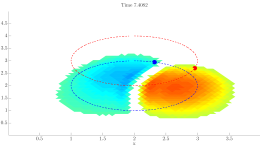
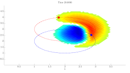
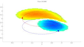
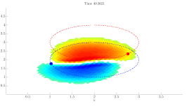
Figure 1: Plots of $\max\{\rho_{1},\rho_{2}\}$ on the $(x,y)$ plane, where $(\rho_{1},\rho_{2})$ solve (3.1)–(3.3)–(3.4). The circles are the fixed trajectories of the guides. The blue refers to $i=1$, while the yellow/red to $i=2$. The blue guide moves clockwise, the other one counterclockwise. The choice (3.4) prevents the mixing of the two groups.

According to (3.3)–(3.4), the groups walk towards their guides and come into contact at $t\approx 7.4$. At $t\approx 20.7$, the blue guide is surrounded by the reds and waits for his group. Meanwhile, the red group bypasses the blues and avoid the congestion. At about $t\approx 28.3$, the groups are separated, while they meet again at $t\approx 40.4$.

3.2 Interacting Crowds and Vehicles

We consider two groups of pedestrians crossing a street at a crosswalk, following [3, 4]. The people near the crosswalk reduce their speed and possibly stop if cars are near to the crosswalk. At the same time, cars slow down and possibly stop as soon as in front of them pedestrians are present. The density $\rho^{i}(t,x)$, for $i=1\ldots,n$, describes the $i$-th group of pedestrians. Each driver’s position can thus be identified through its scalar coordinate $p^{k}$, for $k=1\ldots,N$, along the road. Without loss of generality, we assume that the road is parallel to the vector $[1,0]^{T}$, with width $2h_{R}$, i.e. ${\left|x_{2}-\bar{x}_{2}\right|}\leqslant h_{R}$. Therefore, we have

$$d=2\,,\quad n=2\,,\quad m=N\,,\quad\ell=N\,.$$

The dynamics of the pedestrians is similar to that introduced in [6, 8], namely

$$\partial_{t}\rho^{i}+\nabla_{x}\cdot\left[2\rho^{i}\;(1-\rho^{i})\;w^{i}(x,p)\,\left(V^{i}(x)-\mathcal{A}^{i}(\rho)\right)\right]=0,\qquad i=1,2\,.$$ (3.5)

Here $w^{i}\in\mathbf{C}^{2}({\mathbb{R}}^{d}\times{\mathbb{R}}^{m};{\mathbb{R}}^{+})$ describes the interaction between the member of the $i$-th group located at $x$ and the cars. $\mathcal{A}^{i}$ is chosen as in (3.2) and models the interactions of pedestrians. Finally, the vector field ${V}^{i}\in\mathbf{C}^{2}({\mathbb{R}}^{d};{\mathbb{R}}^{d})$ stands for the preferred trajectories of the people.

The dynamics of cars along the road is described by the Follow The Leader model

$$\left\{\begin{array}[]{rcl}\dot{p}^{k}&=&g\!\left(\left(\mathcal{B}(\rho)\right)(p^{k})\right)\;u(p^{k+1}-p^{k}),\qquad k=1,\ldots,m-1,\\ \dot{p}^{m}&=&v_{L}(t),\end{array}\right.$$ (3.6)

where the non increasing function $g\in\mathbf{C}^{2}({\mathbb{R}};[0,1])$ describes the slowing of cars when near to pedestrians while the non decreasing function $u\in\mathbf{C}^{2}({\mathbb{R}};[0,1])$ vanishes on ${\mathbb{R}}^{-}$ and describes the usual drivers’ behavior in Follow The Leader models. The assigned function $v_{L}=v_{L}(t)$ is the speed of the leader, i.e., of the first vehicle. For simplicity, we assume that the initial position of the first car is after the crosswalk so that its subsequent dynamics is independent from the crowds.

The present model fits into the framework presented in Section 2 by setting

$$\begin{array}[]{@{}r@{\,}c@{\,}lr@{\,}c@{\,}l@{}}q^{1}(\rho^{1})&=&2\rho^{1}(1-\rho^{1}),&q^{2}(\rho^{2})&=&2\rho^{2}(1-\rho^{2}),\\ v^{1}(t,x,A,p)&=&w^{1}(x,p)\left(V^{1}(x)-A\right),&v^{2}(t,x,A,p)&=&w^{2}(x,p)\left(V^{2}(x)-A\right),\\ \mathcal{A}^{1}(\rho)&=&\displaystyle\sum_{j=1}^{2}\frac{\varepsilon_{1j}\,\nabla_{x}(\rho^{j}\ast\eta)}{\sqrt{1+{\left\|\nabla_{x}(\rho^{j}\ast\eta)\right\|}_{{\mathbb{R}}^{2}}^{2}}},&\mathcal{A}^{2}(\rho)&=&\displaystyle\sum_{j=1}^{2}\frac{\varepsilon_{2j}\,\nabla_{x}(\rho^{j}\ast\eta)}{\sqrt{1+{\left\|\nabla_{x}(\rho^{j}\ast\eta)\right\|}_{{\mathbb{R}}^{2}}^{2}}},\end{array}$$ (3.7)

$$\begin{array}[]{@{}rcl@{}}F_{k}(t,p,B)&=&\left\{\begin{array}[]{l@{\qquad\qquad}r@{\;}c@{\;}l@{}}g(B)\;u(p_{1}^{k+1}-p_{1}^{k}),&k&=&1,\ldots,m-1,\\ v_{L}(t),&k&=&m,\end{array}\right.\\ \left(\mathcal{B}(\rho)\right)(p^{k})&=&\displaystyle\int_{{\mathbb{R}}^{2}}\left(\rho^{1}(x)+\rho^{2}(x)\right)\;\bar{\eta}\!\left(x-\left[\begin{array}[]{@{}c@{}}p^{k}\\ \bar{x}_{2}\end{array}\right]\right)\,\mathinner{\mathrm{d}{x}},\quad k=1,\ldots,m\,.\!\!\!\!\end{array}$$ (3.8)

Proposition 3.2.

Assume $\eta,\bar{\eta}\in\mathbf{C}_{c}^{2}({\mathbb{R}}^{2};{\mathbb{R}}^{+})$, $w^{i}\in\mathbf{C}^{2}({\mathbb{R}}^{2}\times{\mathbb{R}}^{2N};{\mathbb{R}}^{+})$, $V^{i}\in\mathbf{C}^{2}\left({\mathbb{R}}^{2};{\mathbb{R}}^{2}\right)$, $v_{L}\in{\mathbf{L}^{1}}({\mathbb{R}}^{+};{\mathbb{R}}^{+})$ and $g,u\in\mathbf{C}^{2}\left({\mathbb{R}};[0,1]\right)$. Then, the functions defined in (3.7)–(3.8) satisfy (v.1), (F), ($\boldsymbol{\mathcal{A}}$), ($\boldsymbol{\mathcal{B}}$) and (q). In particular, Corollary 2.3 applies to (3.5)-(3.6).

The proof is deferred to Section 4.

As a specific example we consider the spatial domain $\mathcal{D}=[0,1]\times[0,1]$, with a road occupying the region $\mathcal{R}=[0,1]\times[0.45,0.55]$ (so that $\bar{x}_{2}=0.5$ and $h_{R}=0.05$) and the crosswalk $\mathcal{C}=[0.4,0.6]\times[0.45,0.55]$. Therefore, pedestrians may walk in $\mathcal{C}\cup(\mathcal{D}\setminus\mathcal{R})$, while cars travel along $\mathcal{R}$ from left to right. The $\rho^{1}$ population targets the bottom boundary $[0,1]\times\{0\}$, while $\rho^{2}$ points towards the top boundary $[0,1]\times\{1\}$, see Figure 2. No individual is allowed to cross the road aside the crosswalk.

The vector $V^{1}(x)$, respectively $V^{2}(x)$, is chosen with norm $1$ and tangent to the geodesic path at $x$ for the population $1$, respectively $2$. In general, these vectors can be computed as solutions to the eikonal equation and their regularity depends on the geometry of the domain[18].

First, for $\alpha_{1}<\alpha_{2}$, we introduce the smooth function $\beta_{\alpha_{1},\alpha_{2}}\in\mathbf{C}^{\infty}({\mathbb{R}};[0,1])$ defined as
$$\hfill\beta_{\alpha_{1},\alpha_{2}}(z)=\left\{\begin{array}[]{@{}lr@{\,}c@{\,}l@{}}1,&z&<&\alpha_{1},\\ \exp\left[1-\left(1-\left(\frac{z-\alpha_{1}}{\alpha_{2}-\alpha_{1}}\right)^{2}\right)^{-1}\right],&z&\in&[\alpha_{1},\alpha_{2}],\\ 0,&z&>&\alpha_{2}\,.\end{array}\right.$$
For $i=1,2$ we choose

$$w^{i}(x,p) = 1-\left(1-\beta_{h_{R},h_{R}+\varepsilon_{\gamma}}({\left|x_{2}-\bar{x}_{2}\right|})\right)\!\left[1-\prod_{l=1}^{3}\beta_{r_{i},r_{a}}\left(\hat{\eta}^{i}\left(x,\left[\begin{array}[]{@{}c@{}}p^{l}\\ \bar{x}_{2}\end{array}\right]\right)\right)\right],\quad\begin{array}[]{@{}r@{\,}c@{\,}l@{}}\bar{x}_{2}&=&0.5,\\ h_{R}&=&0.05,\\ \varepsilon_{\gamma}&=&0.001,\\ r_{i}&=&0.1,\\ r_{a}&=&0.8,\\ \end{array}$$

$$\hat{\eta}^{i}(x,p) = \left\{\begin{array}[]{@{}ll@{}}\eta_{3}\!\left((p-x)\cdot V^{i}(x),r_{v}\right)\;\eta_{3}\!\left((p-x)\cdot V^{i}(x)^{\perp},r_{v}\right),&(p-x)\cdot V^{i}(x)>0,\\ \eta_{3}\!\left((p-x)\cdot V^{i}(x),r_{vb}\right)\;\eta_{3}\!\left((p-x)\cdot V^{i}(x)^{\perp},r_{v}\right),&\mbox{otherwise,}\end{array}\right.$$

$$\eta_{3}(z,r) = \left\{\begin{array}[]{@{}ll@{}}\exp\left(-\frac{z^{2}}{r^{2}-z^{2}}\right),&z\in[-r,r],\\ 0,&\mbox{otherwise,}\end{array}\right.\qquad\qquad\qquad\qquad\qquad\begin{array}[]{@{}r@{\,}c@{\,}l@{}}r_{v}&=&0.15,\\ r_{vb}&=&0.0015.\end{array}$$

Here, $\hat{\eta}_{i}$ describes the region considered by each pedestrian in reacting to cars. For instance, cars behind a pedestrian are ignored when at a distance greater than $r_{vb}$, while cars in front of the pedestrian are considered up to a distance $r_{v}$. Outside the interval defined by the threshold parameters $r_{i}$ and $r_{a}$, the pedestrians’ sensitivity to cars is amplified.

The convolution kernel in the nonlocal operators $\mathcal{A}^{1}$ and $\mathcal{A}^{2}$ are

$$\tilde{\eta}_{r}(x)=\left\{\begin{array}[]{@{}ll@{}}\exp\left(-\frac{5{x_{1}}^{2}}{r^{2}-{x_{1}}^{2}}-\frac{5{x_{2}}^{2}}{r^{2}-{x_{2}}^{2}}\right),&x\in[-r,r]^{2},\\ 0,&\mbox{otherwise,}\end{array}\right.\qquad\eta(x)=\frac{\tilde{\eta}_{r}(x)}{\int_{{\mathbb{R}}^{2}}\tilde{\eta}_{r}(x)\mathinner{\mathrm{d}{x}}},\quad\qquad r=0.05\,.$$

with interaction parameters

$$\varepsilon_{11}=0.1\,,\qquad\varepsilon_{22}=0.1\,,\qquad\varepsilon_{12}=0.7\,,\qquad\varepsilon_{21}=0.7\,.$$

In the Follow The Leader model, we choose $N=3$ vehicles and let

$$v_{L}(t)=1\,,\qquad g(B)=\beta_{r_{j},r_{b}}(B),\quad\mbox{ and }\quad u(\xi)=1-\beta_{H,10H}(\xi)^{K},\quad\mbox{ with }\quad\begin{array}[]{@{}r@{\,}c@{\,}l@{}}r_{j}&=&0.125,\\ r_{b}&=&0.5,\\ H&=&0.167,\\ K&=&50.\end{array}$$

The microscopic model for vehicles is completed by the convolution kernel in the nonlocal operator $\mathcal{B}$

$$\tilde{\eta_{2}}(x)=\left\{\begin{array}[]{ll}\eta_{R}(x),&x_{1}>0,\\ \eta_{R^{\prime}}(x_{1},0)\;\eta_{R}(0,x_{2}),&\mbox{otherwise,}\end{array}\right.\qquad\quad\bar{\eta}(x)=\frac{\tilde{\eta}_{2}(x)}{\int_{{\mathbb{R}}^{2}}\tilde{\eta}_{2}(x)\mathinner{\mathrm{d}{x}}},\qquad\quad\begin{array}[]{@{}r@{\,}c@{\,}l@{}}R&=&0.045,\\ R^{\prime}&=&0.0045\,.\end{array}$$

As initial condition we prescribe

$$\begin{array}[]{rcl}\rho_{0}^{1}&=&\chi_{[0.1,0.9]\times[0.7,0.9]},\\ \rho_{0}^{2}&=&0.5\,\chi_{[0.1,0.9]\times[0.1,0.3]},\end{array}\qquad\mbox{ and }\qquad\begin{array}[]{rcl}p_{o}^{1}&=&0.000,\\ p_{o}^{2}&=&0.333,\\ p_{o}^{3}&=&0.667\,.\end{array}$$

In Figure 2 the maximal density $\rho_{m}=\max(\rho^{1},\rho^{2})$ of the two groups is shown. The first group is illustrated in blue and the second one in red.

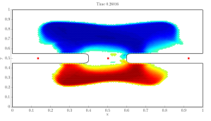
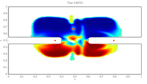
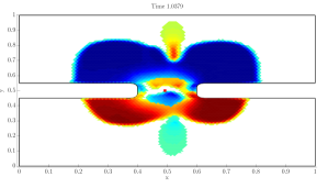
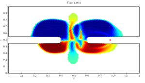
Figure 2: Plots of $\max\{\rho_{1},\rho_{2}\}$ on the $(x,y)$ plane, where $(\rho_{1},\rho_{2})$ solve (3.5)–(3.6)–(3.7)–(3.8). The blue population $\rho_{1}$ moves downward; the red one, $\rho_{2}$. upward. Cars are represented by the red dots along the road. Above: left, pedestrians wait until the second car has passed the crosswalk; right, pedestrians cross the road and form lanes. Bottom: left, pedestrians wait until the third car has passed the crosswalk; right, pedestrians cross the road and form lanes.

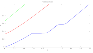
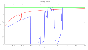
Figure 3: Positions, left, and velocities, right, of the cars in the solution to (3.5)–(3.6)–(3.7)–(3.8) as a function of time, on the horizontal axes. The green lines refer to $p_{3}$, the red ones to $p_{2}$ and the blue one to $p_{1}$.

Initially the pedestrians start walking towards the crosswalk and the cars can drive freely. The first car has maximal speed $1$ and the other ones adapt their speed according to the distance to their leading car, see Figure 3. At time $t\approx 0.2$ the second car is in the middle of the crosswalk and only few pedestrians try to cross the road (Figure 2, top left). When the car has left the crosswalk, the pedestrians start walking and form lanes in order to pass through the other group (Figure 2, top right). When the third car approaches the crosswalk, the pedestrians in front of the crosswalk stop while those on the road can continue their way (Figure 2, bottom left). As the street is not cleared immediately, the car almost has to stop (see Figure 3, left). When it has passed the pedestrians can walk again until all have reached their exits (Figure 2, bottom right).

3.3 The Police Separates Conflicting Hooligans

In this example we consider $n=2$ groups of conflicting hooligans and their interaction with police officers in a $d=2$ dimensional region. For the hooligans we use a model of the form

$$\partial_{t}\rho^{i}+\nabla_{x}\cdot\left[\rho^{i}(1-\rho^{i})\left(-w^{i}(x,p)+\mathcal{A}^{i}(\rho)\right)\right]=0,\qquad i=1,2\,,$$ (3.12)

where $\rho^{i}$ is the density of the $i$-th group. Here $w^{i}\in\mathbf{C}^{2}({\mathbb{R}}^{d}\times{\mathbb{R}}^{m};{\mathbb{R}}^{d})$ describes the preferred direction of the hooligans belonging to the $i$-th group and located at $x$ in presence of the police officers $p^{1},\ldots,p^{N}$. The terms $\mathcal{A}^{1}(\rho),\mathcal{A}^{2}(\rho)$ modify the hooligans’ direction according to their distribution in space. The movement of the $N$ police officers is described by the ODEs

$$\dot{p}^{k}=I_{k}(p)+\mathcal{B}_{k}(\rho),\qquad k=1,\ldots,N,$$ (3.13)

where $p^{k}=[p^{k}_{1},p^{k}_{2}]^{T}$ denotes the position in ${\mathbb{R}}^{2}$ of the $k$-th policeman; so we set $m=2N$. The term $I_{k}\in\mathbf{C}^{0}({\mathbb{R}}^{2N};{\mathbb{R}}^{2})$ avoids concentrations of officers at the same place, while the term $\mathcal{B}_{k}(\rho)$ takes into consideration the distribution of the hooligans.

The present model fits in the framework presented in Section 2 by setting

$$\begin{array}[]{rcl@{\qquad}rcl}q^{1}(\rho)&=&\rho(1-\rho),&q^{2}(\rho)&=&\rho(1-\rho),\\ v^{1}(t,x,A,p)&=&-w^{1}(x,p)+A,&v^{2}(t,x,A,p)&=&-w^{2}(x,p)+A,\\ F_{k}(t,p,B)&=&I_{k}(p)+B_{k},\end{array}$$ (3.14)

$$\begin{array}[]{@{}rcl@{}}\displaystyle\mathcal{A}^{1}(\rho)&=&\displaystyle\frac{\varepsilon_{11}\;\eta\ast(\rho^{1}-\bar{\rho})\;\nabla_{x}(\rho^{1}\ast\eta)}{\sqrt{1+\|\eta\ast(\rho^{1}-\bar{\rho})\nabla_{x}(\rho^{1}\ast\eta)\|^{2}}}+\frac{\varepsilon_{12}\;\eta\ast(\rho^{2}-\rho^{1})\nabla_{x}(\rho^{2}\ast\eta)}{\sqrt{1+\|\eta\ast(\rho^{2}-\rho^{1})\nabla_{x}(\rho^{2}\ast\eta)\|^{2}}},\vspace{.2cm}\\ \displaystyle\mathcal{A}^{2}(\rho)&=&\displaystyle\frac{\varepsilon_{22}\;\eta\ast(\rho^{2}-\bar{\rho})\;\nabla_{x}(\rho^{2}\ast\eta)}{\sqrt{1+\|\eta\ast(\rho^{1}-\bar{\rho})\nabla_{x}(\rho^{2}\ast\eta)\|^{2}}}+\frac{\varepsilon_{21}\;\eta\ast(\rho^{1}-\rho^{2})\nabla_{x}(\rho^{1}\ast\eta)}{\sqrt{1+\|\eta\ast(\rho^{1}-\rho^{2})\nabla_{x}(\rho^{1}\ast\eta)\|^{2}}},\vspace{.2cm}\\ \displaystyle\mathcal{B}_{k}(\rho)(p)&=&\displaystyle\bar{\varepsilon}_{1}\frac{1}{N}\sum_{j=1}^{N}\sum_{l\neq j}\frac{\nabla_{x}((\bar{\eta}\ast\rho^{l})(\bar{\eta}\ast\rho^{j}))(p^{k})}{\sqrt{1+\|\nabla_{x}((\bar{\eta}\ast\rho^{l})(\bar{\eta}\ast\rho^{j}))(p^{k})\|^{2}}}.\end{array}$$ (3.15)

In (3.15), the operator $\mathcal{A}^{i}$ is composed by two terms describing the attraction, respectively repulsion, between members of the same, respectively different, group. Here, we introduce a preferred density $\bar{\rho}\in[0,1]$. If the density of one group is lower than $\bar{\rho}$, then members of that group tend to move towards each other. On the contrary, if the density is bigger than $\bar{\rho}$, then they tend to disperse. Moreover, the operator $\mathcal{A}^{i}$ also models the fact that one group of hooligans aims at attacking the other group as soon as it feels to be stronger. On the contrary, hooligans of a faction try to avoid the adversaries in case they are less represented.

Proposition 3.3.

Let $N\in{\mathbb{N}}\setminus\{0\}$. Assume $\eta,\bar{\eta}\in\mathbf{C}_{c}^{2}({\mathbb{R}}^{2};{\mathbb{R}}^{+})$, $w^{i}\in\mathbf{C}^{2}({\mathbb{R}}^{2}\times{\mathbb{R}}^{2N};{\mathbb{R}}^{2})$, $I_{k}\in(\mathbf{C}^{0}\cap{\mathbf{L}^{\infty}})({\mathbb{R}}^{2N};{\mathbb{R}}^{2})$. Then, the functions defined in (3.14)–(3.15) satisfy (v.1), (F), ($\boldsymbol{\mathcal{A}}$), ($\boldsymbol{\mathcal{B}}$) and (q). In particular, Corollary 2.3 applies to (3.14)–(3.15).

The proof is deferred to Section 4.

As a specific example, in the computational domain $[0,1]^{2}$, we consider $N=4$ policemen, so that $m=8$, and the parameters

$$\varepsilon_{11}=0.5\,,\qquad\varepsilon_{22}=0.5\,,\qquad\varepsilon_{12}=0.5\,,\qquad\varepsilon_{21}=0.5\,,\qquad\bar{\varepsilon}_{1}=0.4\,,\qquad\bar{\rho}=0.5\,,$$

with the functions

$$\begin{array}[]{@{}rclrclrcl@{}}w^{1}(x,p)&=&\displaystyle\frac{\varepsilon_{3}}{N}\sum_{j=1}^{N}\hat{\eta}(x-p^{j})\left[\begin{array}[]{@{}c@{}}0\\ -1\end{array}\right],&\varepsilon_{3}&=&0.1,\\ w^{2}(x,p)&=&\displaystyle\frac{\varepsilon_{4}}{N}\sum_{j=1}^{N}\hat{\eta}(x-p^{j})\left[\begin{array}[]{@{}c@{}}0\\ 1\end{array}\right],&\varepsilon_{4}&=&0.1,\\ I_{k}(p)&=&\displaystyle\frac{\bar{\varepsilon}_{2}}{N}\sum_{j=1}^{N}\frac{\nabla_{x}\tilde{\eta}(p^{j}-p^{k})}{\sqrt{1+\|\nabla_{x}\tilde{\eta}(p^{j}-p^{k})\|^{2}}},&\bar{\varepsilon}_{2}&=&0.2\,,&k&=&1,\ldots,N\,.\end{array}$$

Moreover, we let

$$\begin{array}[]{rcl@{\mbox{ with }}r}\eta_{r}(x)&=&\left\{\begin{array}[]{ll@{}}\exp\left(-\frac{5{x_{1}}^{2}}{r^{2}-{x_{1}}^{2}}-\frac{5{x_{2}}^{2}}{r^{2}-{x_{2}}^{2}}\right),&x\in[-r,r]^{2},\\ 0,&\mbox{otherwise,}\end{array}\right.&\begin{array}[]{rcl@{}}\eta(x)&=&\frac{\eta_{0.1}(x)}{\int_{{\mathbb{R}}^{2}}\eta_{0.1}(x)\mathinner{\mathrm{d}{x}}}\,,\\ \hat{\eta}(x)&=&\frac{\eta_{0.15}(x)}{\int_{{\mathbb{R}}^{2}}\eta_{0.15}(x)\mathinner{\mathrm{d}{x}}}\,,\end{array}\\ \tilde{\eta}_{r}(x)&=&\left\{\begin{array}[]{ll@{}}\left[\left(1-\frac{x_{1}}{r})^{2}\right)\left(1-\frac{x_{2}}{r})^{2}\right)\right]^{3},&x\in[-r,r]^{2},\\ 0,&\mbox{otherwise,}\end{array}\right.&\begin{array}[]{rcl@{}}\bar{\eta}(x)&=&\frac{\tilde{\eta}_{0.1}(x)}{\int_{{\mathbb{R}}^{2}}\tilde{\eta}_{0.1}(x)\mathinner{\mathrm{d}{x}}}\,,\\ \tilde{\eta}(x)&=&\frac{\tilde{\eta}_{0.2}(x)}{\int_{{\mathbb{R}}^{2}}\tilde{\eta}_{0.2}(x)\mathinner{\mathrm{d}{x}}}\,.\end{array}\end{array}$$

For the numerical example, the initial conditions are

$$\begin{array}[]{rcl}\rho_{0}^{1}&=&0.9\;\chi_{[0.25,0.75]\times[0.2,0.5]},\\ \rho_{0}^{2}&=&0.7\;\chi_{[0.25,0.75]\times[0.5,0.8]},\end{array}\qquad\mbox{ and }\qquad\begin{array}[]{rcl}p_{o}^{1}&=&[0.1,0.7]^{T},\\ p_{o}^{2}&=&[0.9,0.3]^{T},\\ p_{o}^{3}&=&[0.1,0.4]^{T},\\ p_{o}^{4}&=&[0.9,0.7]^{T}\,.\end{array}$$ (3.16)

In the pictures below the density of the two groups are plotted separately. The police officers are indicated by green circles.

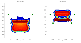
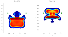
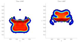
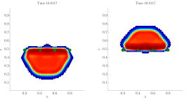
Figure 4: Plots of the solution to (3.12)–(3.13)–(3.16) on the $(x,y)$ plane. In each of the four pairs of diagrams, $\rho_{1}$ is on the left and $\rho_{2}$ is on the right. Above left: two groups of hooligans start fighting. Above right: two officers start to separate the fighting groups. Bottom left: the officers succeed in separating the groups in the central part, but fighting continues on the sides. Bottom right: the four officers succeed in separating the two groups.

At the beginning the two groups of hooligans start fighting in the middle of the domain, while some part of the groups split from the rest and stay calm (Figure 4, top left). As the conflicting groups mix, the police approaches and tries to separate them. The first two officers can not completely isolate the groups (Figure 4, top right) as at the boundaries the hooligans still attack. This stops when the other two policemen join the line of officers (Figure 4, bottom left). At the end the police can separate the conflicting parties (Figure 4, bottom right). This latter configuration appears to be relatively stationary.

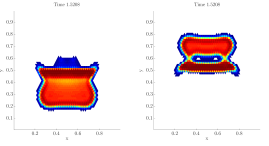
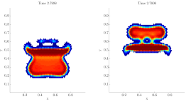
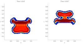
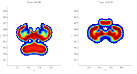
Figure 5: Plots of the solution to (3.12)–(3.13)–(3.16) on the $(x,y)$ plane, but with $\varepsilon_{3}=\varepsilon_{4}=0$, so that police officers are absent. Note that, differently from the integration shown in Figure 4, here the two groups are superimposed, meaning that a fight takes place. In each of the four pairs of diagrams, $\rho_{1}$ is on the left and $\rho_{2}$ is on the right.

The same equations, but with no police officers so that $\varepsilon_{3}=\varepsilon_{4}=0$, is displayed in Figure 5. Note that the two groups superimpose and in the region occupied by both a fight takes place.

4 Technical Details

Denote $W_{d}=\int_{0}^{\pi/2}\left(\cos(\vartheta)\right)^{d}\mathinner{\mathrm{d}{\vartheta}}$. For later use, we state here without proof the Grönwall type lemma used in the sequel.

Lemma 4.1.

Let $T>0$, $\delta\in\mathbf{C}^{0}\left([0,T];{\mathbb{R}}^{+}\right)$, $\alpha\in{\mathbf{L}_{loc}^{\infty}}\left([0,T];{\mathbb{R}}^{+}\right)$ and $\beta\in{\mathbf{L}_{loc}^{1}}([0,T];\mathaccent 23{{\mathbb{R}}}^{+})$. If $\displaystyle\delta(t)\leqslant\alpha(t)+\int_{0}^{t}\beta(\tau)\,\delta(\tau)\mathinner{\mathrm{d}{\tau}}$ for a.e. $t\in[0,T]$ then,

$$\delta(t)\leqslant\alpha(t)+\int_{0}^{t}\alpha(\tau)\,\beta(\tau)\,e^{\int_{\tau}^{t}\beta(s)\,\mathinner{\mathrm{d}{s}}}\,\mathinner{\mathrm{d}{\tau}}\leqslant\left(\sup_{\tau\in[0,t]}\alpha(\tau)\right)\;e^{\int_{0}^{t}\beta(\tau)\,\mathinner{\mathrm{d}{\tau}}}\,,\quad\text{for a.e.~{}$t\in[0,T]$.}$$

The proof is immediate and hence omitted.

The well posedness of the Cauchy problem

$$\left\{\begin{array}[]{l}\partial_{t}\rho+\nabla_{x}\cdot\left(q(\rho)V(t,x)\right)=0,\\ \rho(0,x)=\rho_{o}(x).\end{array}\right.$$ (4.1)

follows from [14, Proposition 2.9].

Lemma 4.2.

Assume $R>0$ and

$$q \in \mathbf{C}^{2}({\mathbb{R}}^{+};{\mathbb{R}}^{+})\textrm{ satisfies }q(0)=0\textrm{ and }q(R)=0,$$ (4.2)

$$V \in \mathbf{C}^{2}({\mathbb{R}}^{+}\times{\mathbb{R}}^{d};{\mathbb{R}}^{d})\textrm{ satisfies }\left\{\begin{array}[]{l}\nabla_{x}\cdot V(t,\cdot)\in{\mathbf{W}^{1,1}}({\mathbb{R}}^{d};{\mathbb{R}}^{d}),\\ V(t,\cdot)\in{\mathbf{W}^{1,\infty}}({\mathbb{R}}^{d};{\mathbb{R}}^{d}),\end{array}\right.\textrm{ for }t\in{\mathbb{R}}^{+},$$ (4.5)

$$\rho_{o} \in {\mathbf{L}^{1}}({\mathbb{R}}^{d};[0,R]).$$ (4.6)

Then, there exists a unique Kružkov solution $\rho\in\mathbf{C}^{0}\left({\mathbb{R}}^{+};{\mathbf{L}^{1}}({\mathbb{R}}^{d};[0,R])\right)$ to (4.1) and

$${\left\|\rho(t)\right\|}_{{\mathbf{L}^{1}}}={\left\|\rho_{o}\right\|}_{{\mathbf{L}^{1}}}\qquad\mbox{for all }t\in{\mathbb{R}}^{+}\,.$$ (4.7)

If moreover $\rho_{o}\in\mathbf{BV}({\mathbb{R}}^{d};[0,R])$, then, for every $t>0$

$$\mathinner{\rm TV}\left(\rho(t)\right)\leqslant\left(\mathinner{\rm TV}\left(\rho_{o}\right)+d\,W_{d}{\left\|q\right\|}_{{\mathbf{L}^{\infty}}}\int_{0}^{t}\int_{{\mathbb{R}}^{d}}{\left\|\nabla_{x}\nabla_{x}\cdot V(\tau,x)\right\|}_{{\mathbb{R}}^{d}}\mathinner{\mathrm{d}{x}}\mathinner{\mathrm{d}{\tau}}\right)e^{\kappa_{o}\,t},$$ (4.8)

and for every $0<t_{1}<t_{2}$,

$$\begin{array}[]{rcl}\displaystyle{\left\|\rho(t_{2})-\rho(t_{1})\right\|}_{{\mathbf{L}^{1}}}&\leqslant&\displaystyle{\left\|q\right\|}_{{\mathbf{L}^{\infty}}}\int_{t_{1}}^{t_{2}}\int_{{\mathbb{R}}^{d}}{\left|\nabla_{x}\cdot V(t,x)\right|}\mathinner{\mathrm{d}{x}}\mathinner{\mathrm{d}{t}}\\[16.0pt] &&\displaystyle+(t_{2}-t_{1}){\left\|q^{\prime}\right\|}_{{\mathbf{L}^{\infty}}}{\left\|V\right\|}_{{\mathbf{L}^{\infty}}}\sup_{\tau\in[0,t_{2}]}\mathinner{\rm TV}\left(\rho(\tau)\right),\end{array}$$ (4.9)

where $\kappa_{o}=(2d+1){\left\|q^{\prime}\right\|}_{{\mathbf{L}^{\infty}}}{\left\|\nabla_{x}V\right\|}_{{\mathbf{L}^{\infty}}}$.

Let $q_{1}$, $q_{2}$, $V_{1}$, $V_{2}$ and $\rho_{o}^{1}$, $\rho_{o}^{2}$ satisfy (4.2), (4.5) and (4.6). Call $\rho_{1}$, $\rho_{2}$ the solutions to

$$\left\{\begin{array}[]{l}\partial_{t}\rho_{1}+\nabla_{x}\cdot\left(q_{1}(\rho_{1})V_{1}(t,x)\right)=0,\\ \rho_{1}(0,x)=\rho_{o}^{1}(x),\end{array}\right.\textrm{ and }\left\{\begin{array}[]{l}\partial_{t}\rho_{2}+\nabla_{x}\cdot\left(q_{2}(\rho_{2})V_{2}(t,x)\right)=0,\\ \rho_{2}(0,x)=\rho_{o}^{2}(x).\end{array}\right.$$ (4.10)

Then, for every $t\in{\mathbb{R}}^{+}$,

$${\left\|\rho_{1}(t)-\rho_{2}(t)\right\|}_{{\mathbf{L}^{1}}}\!\!\! \leqslant \!\!\!{\left\|\rho_{o}^{1}-\rho_{o}^{2}\right\|}_{{\mathbf{L}^{1}}}e^{\kappa t}$$

$$+ \!\!\!\frac{\kappa_{o}e^{\kappa_{o}t}-\kappa e^{\kappa t}}{\kappa_{o}-\kappa}\left[\mathinner{\rm TV}(\rho_{o}^{1})+d\,W_{d}{\left\|q_{1}\right\|}_{{\mathbf{L}^{\infty}}}{\left\|\nabla_{x}\nabla_{x}\cdot V_{1}\right\|}_{{\mathbf{L}^{1}}([0,t];{\mathbf{L}^{1}})}\right]$$

$$\quad\times\left[{\left\|q^{\prime}_{2}\right\|}_{{\mathbf{L}^{\infty}}}{\left\|V_{1}-V_{2}\right\|}_{{\mathbf{L}^{1}}([0,t];{\mathbf{L}^{\infty}})}+{\left\|q^{\prime}_{1}-q^{\prime}_{2}\right\|}_{{\mathbf{L}^{\infty}}}{\left\|V_{1}\right\|}_{{\mathbf{L}^{1}}([0,t];{\mathbf{L}^{\infty}})}\right]$$

$$+ \!\!\!\!\!\left[{\left\|q_{1}\right\|}_{{\mathbf{L}^{\infty}}}{\left\|\nabla_{x}\cdot(V_{1}-V_{2})\right\|}_{{\mathbf{L}^{1}}([0,t];{\mathbf{L}^{1}})}+{\left\|q_{1}-q_{2}\right\|}_{{\mathbf{L}^{\infty}}}{\left\|\nabla_{x}\cdot V_{2}\right\|}_{{\mathbf{L}^{1}}([0,t];{\mathbf{L}^{1}})}\right]e^{\kappa t}\!,$$

where

$$\begin{array}[]{rcl}\kappa_{o}&=&\displaystyle(2d+1){\left\|q^{\prime}_{1}\right\|}_{{\mathbf{L}^{\infty}}}{\left\|\nabla_{x}V_{1}\right\|}_{{\mathbf{L}^{\infty}}([0,t],{\mathbf{L}^{\infty}})},\\ \kappa&=&\displaystyle{\left\|q_{1}^{\prime}\,\nabla_{x}\cdot V_{1}-q_{2}^{\prime}\,\nabla_{x}\cdot V_{2}\right\|}_{{\mathbf{L}^{\infty}}}.\end{array}$$ (4.11)

Proof.  The equality (4.7) directly follows from (q) and [13, Theorem 1]. The total variation bound (4.8) follows from [14, Theorem 2.2]. Estimate (4.9) follows from [14, Corollary 2.4]. The stability estimate follows from [14, Proposition 2.9].   $\square$

Lemma 4.3.

Assume that (F) and ($\boldsymbol{\mathcal{B}}$) hold. Fix $p_{o}\in{\mathbb{R}}^{m}$ and $r\in\mathbf{C}^{0}\left({\mathbb{R}}^{+};{\mathbf{L}^{1}}({\mathbb{R}}^{d};{\mathbb{R}}^{n})\right)$. Then, problem

$$\left\{\begin{array}[]{l}\dot{p}=F\left(t,p,\left(\mathcal{B}(r)\right)(p)\right),\\ p(0)=p_{o},\end{array}\right.$$

admits a unique Caratheodory solution $p\in{\mathbf{W}^{1,1}}({\mathbb{R}}^{+};{\mathbb{R}}^{m})$ and for every $t>0$

$${\left\|p(t)\right\|}_{{\mathbb{R}}^{m}}\leqslant\left({\left\|p_{o}\right\|}_{{\mathbb{R}}^{m}}+\int_{0}^{t}C_{F}(s)\left(1+L_{B}\,{\left\|r(s)\right\|}_{{\mathbf{L}^{1}}}\right)\mathinner{\mathrm{d}{s}}\right)\exp\left(\int_{0}^{t}C_{F}(s)\mathinner{\mathrm{d}{s}}\right)\,.$$ (4.12)

If $T>0$, $p_{o}^{1},p_{o}^{2}\in{\mathbb{R}}^{m}$ and $r_{1},r_{2}\in\mathbf{C}^{0}\left({\mathbb{R}}^{+};{\mathbf{L}^{1}}({\mathbb{R}}^{d};{\mathbb{R}}^{n})\right)$, calling $p_{1},p_{2}$ the solutions to

$$\left\{\begin{array}[]{l}\dot{p}=F_{1}\left(t,p,\left(\mathcal{B}(r_{1})\right)(p)\right),\\ p(0)=p_{o}^{1},\end{array}\right.\qquad\qquad\left\{\begin{array}[]{l}\dot{p}=F_{2}\left(t,p,\left(\mathcal{B}(r_{2})\right)(p)\right),\\ p(0)=p_{o}^{2},\end{array}\right.$$

for every $t\in[0,T]$ the following estimate holds

$$\begin{array}[]{rcl}{\left\|p_{1}(t)-p_{2}(t)\right\|}_{{\mathbb{R}}^{m}}&\leqslant&\displaystyle\left[{\left\|p_{o}^{1}-p_{o}^{2}\right\|}_{{\mathbb{R}}^{m}}+t{\left\|F_{1}-F_{2}\right\|}_{{\mathbf{L}^{\infty}}}+L_{B}{\left\|r_{1}-r_{2}\right\|}_{{\mathbf{L}^{1}}([0,t];{\mathbf{L}^{1}})}\right]\\ &&\displaystyle\qquad\times e^{L_{F}(t+L_{B}{\left\|r_{1}\right\|}_{{\mathbf{L}^{1}}([0,t];{\mathbf{L}^{1}})})}.\end{array}$$ (4.13)

Proof.  The existence and uniqueness of the solution follows, for instance, from [5, Theorem 2.1.1]. Moreover, by (F) and ($\boldsymbol{\mathcal{B}}$),

$${\left\|p(t)\right\|}_{{\mathbb{R}}^{m}} = {\left\|p_{o}+\int_{0}^{t}F\left(s,p(s),\left(\mathcal{B}(r_{1}(s))\right)\left(p(s)\right)\right)\mathinner{\mathrm{d}{s}}\right\|}_{{\mathbb{R}}^{m}}$$

$$\leqslant {\left\|p_{o}\right\|}_{{\mathbb{R}}^{m}}+\int_{0}^{t}C_{F}(s)\left[1+{\left\|p(s)\right\|}_{{\mathbb{R}}^{m}}+{\left\|\left(\mathcal{B}(r_{1}(s))\right)\left(p(s)\right)\right\|}_{{\mathbb{R}}^{\ell}}\right]\mathinner{\mathrm{d}{s}}$$

$$\leqslant {\left\|p_{o}\right\|}_{{\mathbb{R}}^{m}}+\int_{0}^{t}C_{F}(s)\left(1+L_{B}\,{\left\|r_{1}(s)\right\|}_{{\mathbf{L}^{1}}}\right)\mathinner{\mathrm{d}{s}}+\int_{0}^{t}C_{F}(s){\left\|p(s)\right\|}_{{\mathbb{R}}^{m}}\mathinner{\mathrm{d}{s}}.$$

By Lemma 4.1, we deduce (4.12). To prove the stability estimate, first note that, given $T>0$, by (4.12) there exists a compact set $K\subseteq{\mathbb{R}}^{m}$ such that $p_{1}(t),p_{2}(t)\in K$ for every $t\in[0,T]$. Denote with $L_{F}$ the constant related to $K$ in (F). Using (F) and ($\boldsymbol{\mathcal{B}}$) we get

$${\left\|p_{1}(t)-p_{2}(t)\right\|}_{{\mathbb{R}}^{m}}$$

$$\leqslant {\left\|p_{o}^{1}-p_{o}^{2}\right\|}_{{\mathbb{R}}^{m}}$$

$$+\int_{0}^{t}{\left\|F_{1}\left(\tau,p_{1}(\tau),\left(\mathcal{B}(r_{1})\right)\left(p_{1}(\tau)\right)\right)-F_{2}\left(\tau,p_{1}(\tau),\left(\mathcal{B}(r_{1})\right)\left(p_{1}(\tau)\right)\right)\right\|}_{{\mathbb{R}}^{m}}\mathinner{\mathrm{d}{\tau}}$$

$$+\int_{0}^{t}{\left\|F_{2}\left(\tau,p_{1}(\tau),\left(\mathcal{B}(r_{1})\right)\left(p_{1}(\tau)\right)\right)-F_{2}\left(\tau,p_{1}(\tau),\left(\mathcal{B}(r_{1})\right)\left(p_{2}(\tau)\right)\right)\right\|}_{{\mathbb{R}}^{m}}\mathinner{\mathrm{d}{\tau}}$$

$$+\int_{0}^{t}{\left\|F_{2}\left(\tau,p_{1}(\tau),\left(\mathcal{B}(r_{1})\right)\left(p_{2}(\tau)\right)\right)-F_{2}\left(\tau,p_{1}(\tau),\left(\mathcal{B}(r_{2})\right)\left(p_{2}(\tau)\right)\right)\right\|}_{{\mathbb{R}}^{m}}\mathinner{\mathrm{d}{\tau}}$$

$$+\int_{0}^{t}{\left\|F_{2}\left(\tau,p_{1}(\tau),\left(\mathcal{B}(r_{2})\right)\left(p_{2}(\tau)\right)\right)-F_{2}\left(\tau,p_{2}(\tau),\left(\mathcal{B}(r_{2})\right)\left(p_{2}(\tau)\right)\right)\right\|}_{{\mathbb{R}}^{m}}\mathinner{\mathrm{d}{\tau}}$$

$$\leqslant {\left\|p_{o}^{1}-p_{o}^{2}\right\|}_{{\mathbb{R}}^{m}}+t{\left\|F_{1}-F_{2}\right\|}_{{\mathbf{L}^{\infty}}}$$

$$+L_{F}\int_{0}^{t}{\left\|\left(\mathcal{B}\left(r_{1}(\tau)\right)\right)\left(p_{1}(\tau)\right)-\left(\mathcal{B}\left(r_{1}(\tau)\right)\right)\left(p_{2}(\tau)\right)\right\|}_{{\mathbb{R}}^{\ell}}\mathinner{\mathrm{d}{\tau}}$$

$$+L_{F}\int_{0}^{t}{\left\|\left(\mathcal{B}\left(r_{1}(\tau)\right)\right)\left(p_{2}(\tau)\right)-\left(\mathcal{B}\left(r_{2}(\tau)\right)\right)\left(p_{2}(\tau)\right)\right\|}_{{\mathbb{R}}^{\ell}}\mathinner{\mathrm{d}{\tau}}$$

$$+L_{F}\int_{0}^{t}{\left\|p_{1}(\tau)-p_{2}(\tau)\right\|}_{{\mathbb{R}}^{m}}\mathinner{\mathrm{d}{\tau}}$$

$$\leqslant {\left\|p_{o}^{1}-p_{o}^{2}\right\|}_{{\mathbb{R}}^{m}}+t{\left\|F_{1}-F_{2}\right\|}_{{\mathbf{L}^{\infty}}}+L_{B}\int_{0}^{t}{\left\|r_{1}(\tau)-r_{2}(\tau)\right\|}_{{\mathbf{L}^{1}}}\mathinner{\mathrm{d}{\tau}}$$

$$+L_{F}\int_{0}^{t}\left(1+L_{B}{\left\|r_{1}(\tau)\right\|}_{{\mathbf{L}^{1}}}\right){\left\|p_{1}(\tau)-p_{2}(\tau)\right\|}_{{\mathbb{R}}^{m}}\mathinner{\mathrm{d}{\tau}}\,.$$

Apply Lemma 4.1 to complete the proof.   $\square$

Proof of Theorem 2.2.  The proof is divided in various steps.

Introduction of $X$ and $\mathcal{T}$.

Fix the initial data $(\rho_{o},p_{o})\in({\mathbf{L}^{1}}\cap\mathbf{BV})({\mathbb{R}}^{d};[0,R]^{n})\times{\mathbb{R}}^{m}$ and a positive $T<1$. For positive $\Delta_{\rho},\Delta_{p}$, define the closed balls

$$B_{\rho}=\left\{\rho\in{\mathbf{L}^{1}}({\mathbb{R}}^{d};[0,R]^{n})\colon{\left\|\rho-\rho_{o}\right\|}_{{\mathbf{L}^{1}}}\leqslant\Delta_{\rho}\right\}\quad\mbox{ and }\quad B_{p}=\left\{p\in{\mathbb{R}}^{m}\colon{\left\|p-p_{o}\right\|}_{{\mathbb{R}}^{m}}\leqslant\Delta_{p}\right\}$$

and the space

$$X=\mathbf{C}^{0}([0,T];B_{\rho}\times B_{p})$$

which is a complete metric space with the distance

$$d\left(\left(\rho_{1},p_{1}\right),\left(\rho_{2},p_{2}\right)\right)=\sup_{t\in[0,T]}{\left\|\rho_{1}(t)-\rho_{2}(t)\right\|}_{{\mathbf{L}^{1}}}+\sup_{t\in[0,T]}{\left\|p_{1}(t)-p_{2}(t)\right\|}_{{\mathbb{R}}^{m}}.$$

Consider the function $\mathcal{T}\colon X\to X$, with $\mathcal{T}(r,\pi)=(\rho,p)$, if $(\rho,p)$ is the solution to

$$\left\{\begin{array}[]{l@{\qquad}l}\partial_{t}\rho^{i}+\nabla_{x}\cdot\left[q^{i}(\rho^{i})\;v^{i}\left(t,x,\mathcal{A}^{i}(r),\pi\right)\right]=0,&i\in\left\{1,\ldots,n\right\},\\ \dot{p}=F\left(t,p,\left(\mathcal{B}(r)\right)(p)\right),\\ \rho^{i}(0,x)=\rho_{o}^{i}(x),&i\in\left\{1,\ldots,n\right\},\\ p(0)=p_{o}\,.\end{array}\right.$$ (4.14)

In the spirit of Definition 2.1, here by solution we mean that $(\rho,p)\in\mathbf{C}^{0}([0,T];{\mathbf{L}^{1}}({\mathbb{R}}^{d};{\mathbb{R}}^{n})\times{\mathbb{R}}^{m})$ satisfies $(\rho,p)(0)=(\rho_{o},p_{o})$ and for all $i=1,\ldots,n$, the following inequality holds

$$\begin{array}[]{@{}l@{}}\displaystyle\int_{0}^{T}\int_{{\mathbb{R}}^{d}}\mathop{\rm sgn}\left(\rho^{i}(t,x)-k\right)\Big{[}\left(\rho^{i}(t,x)-k\right)\partial_{t}\varphi(t,x)\\ \displaystyle\qquad+\left(q^{i}\left(\rho^{i}(t,x)\right)-q^{i}(k)\right)v^{i}\left(t,x,\left(\mathcal{A}^{i}\left(r(t)\right)\right)(x),\pi(t)\right)\nabla_{x}\varphi(t,x)\Big{]}\mathinner{\mathrm{d}{x}}\mathinner{\mathrm{d}{t}}\geqslant 0\end{array}$$ (4.15)

for all $\varphi\in\mathbf{C}_{c}^{1}(\left]0,T\right[\times{\mathbb{R}}^{d};{\mathbb{R}}^{+})$ and for all $k\in{\mathbb{R}}$; while, for the $p$ component,

$$p(t)=p_{o}+\int_{0}^{t}F\left(\tau,p(\tau),\left(\mathcal{B}\left(r(\tau)\right)\right)\left(p(\tau)\right)\right)\mathinner{\mathrm{d}{\tau}}$$ (4.16)

for $t\in[0,T]$. Lemma 4.2 and Lemma 4.3 ensure that (4.14) admits a unique solution.

$\mathcal{T}$ is well defined.

To bound the $p$ component, we use (F), ($\boldsymbol{\mathcal{B}}$) and (4.12)

$${\left\|p(t)-p_{o}\right\|}_{{\mathbb{R}}^{m}}$$

$$\leqslant \int_{0}^{t}{\left\|F\left(s,p(s),\left(\mathcal{B}\left(r(s)\right)\right)\left(p(s)\right)\right)\right\|}_{{\mathbb{R}}^{m}}\mathinner{\mathrm{d}{s}}$$

$$\leqslant \int_{0}^{t}C_{F}(s)\left(1+{\left\|p(s)\right\|}_{{\mathbb{R}}^{m}}+{\left\|\left(\mathcal{B}\left(r(s)\right)\right)\left(p(s)\right)\right\|}_{{\mathbb{R}}^{\ell}}\right)\mathinner{\mathrm{d}{s}}$$

$$\leqslant \int_{0}^{t}C_{F}(s)\left(1+{\left\|p(s)\right\|}_{{\mathbb{R}}^{m}}+L_{B}{\left\|r(s)\right\|}_{{\mathbf{L}^{1}}}\right)\mathinner{\mathrm{d}{s}}$$

$$\leqslant \left(1+L_{B}\left({\left\|\rho_{o}\right\|}_{{\mathbf{L}^{1}}}+\Delta_{\rho}\right)\right)\int_{0}^{t}C_{F}(s)\mathinner{\mathrm{d}{s}}$$

$$+\int_{0}^{t}C_{F}(s)\left({\left\|p_{o}\right\|}_{{\mathbb{R}}^{m}}+\left(1+L_{B}\left({\left\|\rho_{o}\right\|}_{{\mathbf{L}^{1}}}+\Delta_{\rho}\right)\right)\int_{0}^{s}C_{F}(\tau)\mathinner{\mathrm{d}{\tau}}\right)e^{\int_{0}^{s}C_{F}(\tau)\mathinner{\mathrm{d}{\tau}}}\mathinner{\mathrm{d}{s}}$$

and the latter term above can be made smaller than $\Delta_{p}$ if $T$ is sufficiently small.

To obtain similar estimates for the $\rho$ component, we set $V(t,x)=v^{i}\left(t,x,\mathcal{A}^{i}(r),\pi\right)$ for $i=1,\ldots,n$ and compute

$$\nabla_{x}\cdot V(t,x) = \sum_{j=1}^{d}\partial_{x_{j}}v_{j}^{i}\left(t,x,\left(\mathcal{A}^{i}\left(r(t)\right)\right)(x),\pi(t)\right)$$ (4.17)

$$+\sum_{j,h=1}^{d}\nabla_{A_{h}}v_{j}^{i}\left(t,x,\left(\mathcal{A}^{i}\left(r(t)\right)\right)(x),\pi(t)\right)\;\partial_{x_{j}}\left(\mathcal{A}^{i}_{h}\left(r(t)\right)\right)(x)$$

$$= \nabla_{x}\cdot v^{i}\left(t,x,\left(\mathcal{A}^{i}\left(r(t)\right)(x)\right),\pi(t)\right)$$

$$+\partial_{A}v^{i}\left(t,x,\left(\mathcal{A}^{i}\left(r(t)\right)\right)(x),\pi(t)\right)\cdot\nabla_{x}\left(\mathcal{A}^{i}\left(r(t)\right)\right)(x),$$

$$\nabla_{x}\nabla_{x}\cdot V\left(t,x\right) = \nabla_{x}\nabla_{x}\cdot v^{i}\left(t,x,\left(\mathcal{A}^{i}\left(r(t)\right)\right)(x),\pi(t)\right)$$

$$+2\nabla_{x}\cdot\nabla_{A}v^{i}\left(t,x,\left(\mathcal{A}^{i}\left(r(t)\right)\right)(x),\pi(t)\right)\cdot\nabla_{x}\left(\mathcal{A}^{i}\left(r(t)\right)\right)(x)$$

$$+\nabla^{2}_{A}v^{i}\left(t,x,\left(\mathcal{A}^{i}\left(r(t)\right)\right)(x),\pi(t)\right)\cdot\left[\nabla_{x}\left(\mathcal{A}^{i}\left(r(t)\right)\right)(x)\right]^{2}$$

$$+\nabla_{A}v^{i}\left(t,x,\left(\mathcal{A}^{i}\left(r(t)\right)\right)(x),\pi(t)\right)\cdot\nabla^{2}_{x}\left(\mathcal{A}^{i}\left(r(t)\right)\right)(x),$$

and by (v) and ($\boldsymbol{\mathcal{A}}$), setting $K=\overline{B(p_{o},\Delta_{p})}$,

$$\int_{0}^{t}\int_{{\mathbb{R}}^{d}}{\left|\nabla_{x}\cdot V(s,x)\right|}\mathinner{\mathrm{d}{x}}\,\mathinner{\mathrm{d}{s}} \leqslant {\left\|\mathcal{C}_{K}\right\|}_{{\mathbf{L}^{1}}}t+L_{A}{\left\|\mathcal{C}_{K}\right\|}_{{\mathbf{L}^{\infty}}}\int_{0}^{t}{\left\|r(s)\right\|}_{{\mathbf{L}^{1}}}\mathinner{\mathrm{d}{s}}$$ (4.18)

$$\leqslant t\left({\left\|\mathcal{C}_{K}\right\|}_{{\mathbf{L}^{1}}}+L_{A}{\left\|\mathcal{C}_{K}\right\|}_{{\mathbf{L}^{\infty}}}\left({\left\|\rho_{o}\right\|}_{{\mathbf{L}^{1}}}+\Delta_{\rho}\right)\right),$$ (4.19)

$$\int_{0}^{t}\int_{{\mathbb{R}}^{d}}{\left\|\nabla_{x}\nabla_{x}\cdot V(\tau,x)\right\|}_{{\mathbb{R}}^{d}}\mathinner{\mathrm{d}{x}}\mathinner{\mathrm{d}{\tau}}$$ (4.20)

$$\leqslant {\left\|\mathcal{C}_{K}\right\|}_{{\mathbf{L}^{1}}}t+2L_{A}t{\left\|\mathcal{C}_{K}\right\|}_{{\mathbf{L}^{\infty}}}\left({\left\|\rho_{o}\right\|}_{{\mathbf{L}^{1}}}+\Delta_{\rho}\right)+L_{A}^{2}t{\left\|\mathcal{C}_{K}\right\|}_{{\mathbf{L}^{\infty}}}\left({\left\|\rho_{o}\right\|}_{{\mathbf{L}^{1}}}+\Delta_{\rho}\right)^{2}$$

$$+L_{A}t{\left\|\mathcal{C}_{K}\right\|}_{{\mathbf{L}^{\infty}}}\left({\left\|\rho_{o}\right\|}_{{\mathbf{L}^{1}}}+\Delta_{\rho}\right)$$

$$= \left({\left\|\mathcal{C}_{K}\right\|}_{{\mathbf{L}^{1}}}+3L_{A}{\left\|\mathcal{C}_{K}\right\|}_{{\mathbf{L}^{\infty}}}\left({\left\|\rho_{o}\right\|}_{{\mathbf{L}^{1}}}+\Delta_{\rho}\right)+L_{A}^{2}{\left\|\mathcal{C}_{K}\right\|}_{{\mathbf{L}^{\infty}}}\left({\left\|\rho_{o}\right\|}_{{\mathbf{L}^{1}}}+\Delta_{\rho}\right)^{2}\right)t.$$

Proceeding to the $\rho$ component, using (4.9) and (4.8) together with (4.19) and (4.20) above

$${\left\|\rho(t)-\rho_{o}\right\|}_{{\mathbf{L}^{1}}}$$

$$\leqslant \int_{0}^{t}\int_{{\mathbb{R}}^{d}}{\left\|q\right\|}_{{\mathbf{L}^{\infty}}}{\left|\nabla_{x}\cdot V(s,x)\right|}\mathinner{\mathrm{d}{x}}\,\mathinner{\mathrm{d}{s}}+t{\left\|q^{\prime}\right\|}_{{\mathbf{L}^{\infty}}}{\left\|V\right\|}_{{\mathbf{L}^{\infty}}}\sup_{\tau\in[0,t]}\mathinner{\rm TV}\left(\rho(\tau,\cdot)\right)$$

$$\leqslant {\left\|q\right\|}_{{\mathbf{L}^{\infty}}}\int_{0}^{t}\int_{{\mathbb{R}}^{d}}{\left|\nabla_{x}\cdot V(s,x)\right|}\mathinner{\mathrm{d}{x}}\,\mathinner{\mathrm{d}{s}}$$

$$+t{\left\|q^{\prime}\right\|}_{{\mathbf{L}^{\infty}}}{\left\|V\right\|}_{{\mathbf{L}^{\infty}}}\left(\mathinner{\rm TV}\left(\rho_{o}\right)+d\,W_{d}{\left\|q\right\|}_{{\mathbf{L}^{\infty}}\left([0,R]\right)}\int_{0}^{t}\int_{{\mathbb{R}}^{d}}{\left\|\nabla_{x}\nabla_{x}\cdot V(\tau,x)\right\|}_{{\mathbb{R}}^{d}}\mathinner{\mathrm{d}{x}}\mathinner{\mathrm{d}{\tau}}\right)e^{\kappa_{o}\,t}$$

$$\leqslant t\,{\left\|q\right\|}_{{\mathbf{L}^{\infty}}}\left({\left\|\mathcal{C}_{K}\right\|}_{{\mathbf{L}^{1}}}+L_{A}{\left\|\mathcal{C}_{K}\right\|}_{{\mathbf{L}^{\infty}}}\left({\left\|\rho_{o}\right\|}_{{\mathbf{L}^{1}}}+\Delta_{\rho}\right)\right)+t{\left\|\mathcal{C}_{K}\right\|}_{{\mathbf{L}^{\infty}}}{\left\|q^{\prime}\right\|}_{{\mathbf{L}^{\infty}}}\mathinner{\rm TV}(\rho_{o})e^{\kappa_{o}t}$$

$$+t^{2}{\left\|\mathcal{C}_{K}\right\|}_{{\mathbf{L}^{\infty}}}{\left\|q^{\prime}\right\|}_{{\mathbf{L}^{\infty}}}dW_{d}{\left\|q\right\|}_{{\mathbf{L}^{\infty}}}$$

$$\times\left({\left\|\mathcal{C}_{K}\right\|}_{{\mathbf{L}^{1}}}+3L_{A}{\left\|\mathcal{C}_{K}\right\|}_{{\mathbf{L}^{\infty}}}\left({\left\|\rho_{o}\right\|}_{{\mathbf{L}^{1}}}+\Delta_{\rho}\right)+L_{A}^{2}{\left\|\mathcal{C}_{K}\right\|}_{{\mathbf{L}^{\infty}}}\left({\left\|\rho_{o}\right\|}_{{\mathbf{L}^{1}}}+\Delta_{\rho}\right)^{2}\right)e^{\kappa_{o}t},$$

where

$$\kappa_{o} = (2d+1){\left\|q^{\prime}\right\|}_{{\mathbf{L}^{\infty}}}{\left\|\nabla_{x}V\right\|}_{{\mathbf{L}^{\infty}}}$$ (4.21)

$$= (2d+1){\left\|q^{\prime}\right\|}_{{\mathbf{L}^{\infty}}}{\left\|\nabla_{x}v^{i}+\nabla_{A}v^{i}\cdot\nabla_{x}\mathcal{A}^{i}\left(r(t)\right)\right\|}_{{\mathbf{L}^{\infty}}}$$

$$\leqslant (2d+1){\left\|q^{\prime}\right\|}_{{\mathbf{L}^{\infty}}}\left[{\left\|\mathcal{C}_{K}\right\|}_{{\mathbf{L}^{\infty}}}+{\left\|\mathcal{C}_{K}\right\|}_{{\mathbf{L}^{\infty}}}L_{A}{\left\|r(t)\right\|}_{{\mathbf{L}^{1}}}\right]$$

$$\leqslant (2d+1){\left\|\mathcal{C}_{K}\right\|}_{{\mathbf{L}^{\infty}}}{\left\|q^{\prime}\right\|}_{{\mathbf{L}^{\infty}}}\left[1+L_{A}\left({\left\|\rho_{o}\right\|}_{{\mathbf{L}^{1}}}+\Delta_{\rho}\right)\right].$$ (4.22)

Hence, for $T$ sufficiently small, also ${\left\|\rho(t)-\rho_{o}\right\|}_{{\mathbf{L}^{1}}}\leqslant\Delta_{\rho}$ completing the proof that $\mathcal{T}$ is well defined.

Notation.

In the sequel, for notational simplicity, we introduce the Landau symbol $\mathcal{O}(1)$ to denote a bounded quantity, possibly dependent on $T$ and on the constants in (v), (F), ($\boldsymbol{\mathcal{A}}$), ($\boldsymbol{\mathcal{B}}$) and (q).

$\mathcal{T}$ is a contraction.

Fix $(r_{1},\pi_{1}),(r_{2},\pi_{2})\in X$ and denote $(\rho_{i},p_{i})=\mathcal{T}(r_{i},\pi_{i})$. We now estimate $d\left((\rho_{1},p_{1}),(\rho_{2},p_{2})\right)$. Consider first the $p$ component. Using Lemma 4.3 we get

$${\left\|p_{1}(t)-p_{2}(t)\right\|}_{{\mathbb{R}}^{m}} \leqslant L_{B}\,{\left\|r_{1}-r_{2}\right\|}_{{\mathbf{L}^{1}}([0,t];{\mathbf{L}^{1}})}\,e^{L_{F}(t+L_{B}{\left\|r_{1}\right\|}_{{\mathbf{L}^{1}}([0,t];{\mathbf{L}^{1}})})}$$

$$\leqslant L_{B}\,t\,{\left\|r_{1}-r_{2}\right\|}_{\mathbf{C}^{0}([0,t];{\mathbf{L}^{1}})}\,e^{L_{F}t(1+L_{B}({\left\|\rho_{o}\right\|}_{{\mathbf{L}^{1}}}+\Delta_{\rho}))}$$

$$= \mathcal{O}(1)\,t\,{\left\|r_{1}-r_{2}\right\|}_{\mathbf{C}^{0}([0,t];{\mathbf{L}^{1}})}.$$

Apply now Lemma 4.2 with $\rho_{o}^{1}=\rho_{o}=\rho_{o}^{2}$, $q_{1}=q=q_{2}$, $V_{j}^{i}(t,x)=v^{i}\left(t,x,\mathcal{A}^{i}(r_{j}(t)(x),\pi_{j}(t)\right)$ for $i=1,\ldots,n$ and $j=1,2$. Equality (4.17) and (v) allow to bound $\kappa$ in (4.11) as follows

$$\kappa\leqslant{\left\|q^{\prime}\right\|}_{{\mathbf{L}^{\infty}}}{\left\|\nabla_{x}\cdot(V^{i}_{1}-V^{i}_{2})\right\|}_{{\mathbf{L}^{\infty}}}\leqslant 2\,{\left\|\mathcal{C}_{K}\right\|}_{{\mathbf{L}^{\infty}}}\,{\left\|q^{\prime}\right\|}_{{\mathbf{L}^{\infty}}}\left(1+L_{A}\left({\left\|\rho_{o}\right\|}_{{\mathbf{L}^{1}}}+\Delta_{\rho}\right)\right),$$

which ensures, together with (4.22)

$$\frac{\kappa_{o}e^{\kappa_{o}t}-\kappa e^{\kappa t}}{\kappa_{o}-\kappa} \leqslant \left(1+(2d+1){\left\|\mathcal{C}_{K}\right\|}_{{\mathbf{L}^{\infty}}}{\left\|q^{\prime}\right\|}_{{\mathbf{L}^{\infty}}}\left[1+L_{A}\left({\left\|\rho_{o}\right\|}_{{\mathbf{L}^{1}}}+\Delta_{\rho}\right)\right]t\right)$$

$$\times\exp\left((2d+1){\left\|\mathcal{C}_{K}\right\|}_{{\mathbf{L}^{\infty}}}{\left\|q^{\prime}\right\|}_{{\mathbf{L}^{\infty}}}\left[1+L_{A}\left({\left\|\rho_{o}\right\|}_{{\mathbf{L}^{1}}}+\Delta_{\rho}\right)\right]t\right)$$

$$= \mathcal{O}(1)\,.$$

Using also (4.20) we obtain

$$\!\!\!{\left\|\rho_{1}^{i}(t)-\rho_{2}^{i}(t)\right\|}_{{\mathbf{L}^{1}}}$$

$$\leqslant \!\!\!t\frac{\kappa_{o}e^{\kappa_{o}t}-\kappa e^{\kappa t}}{\kappa_{o}-\kappa}\!\left[\mathinner{\rm TV}(\rho_{o})+d\,W_{d}{\left\|q\right\|}_{{\mathbf{L}^{\infty}}}{\left\|\nabla_{x}\nabla_{x}\cdot V_{1}^{i}\right\|}_{{\mathbf{L}^{1}}([0,t];{\mathbf{L}^{1}})}\right]\!\!{\left\|q^{\prime}\right\|}_{{\mathbf{L}^{\infty}}}{\left\|V_{1}^{i}-V_{2}^{i}\right\|}_{\mathbf{C}^{0}([0,t];{\mathbf{L}^{\infty}})}$$

$$\!\!\!+{\left\|q\right\|}_{{\mathbf{L}^{\infty}}}{\left\|\nabla_{x}\cdot(V_{1}^{i}-V_{2}^{i})\right\|}_{{\mathbf{L}^{1}}([0,t];{\mathbf{L}^{1}})}e^{\kappa t}$$

$$= \!\!\!t\mathcal{O}(1)\left[1+{\left\|\nabla_{x}\nabla_{x}\cdot V_{1}^{i}\right\|}_{{\mathbf{L}^{1}}([0,t];{\mathbf{L}^{1}})}\right]{\left\|V_{1}^{i}-V_{2}^{i}\right\|}_{\mathbf{C}^{0}([0,t];{\mathbf{L}^{\infty}})}+\mathcal{O}(1){\left\|\nabla_{x}\cdot(V_{1}^{i}-V_{2}^{i})\right\|}_{{\mathbf{L}^{1}}([0,t];{\mathbf{L}^{1}})}.$$

By (4.20), we get ${\left\|\nabla_{x}\nabla_{x}\cdot V_{1}^{i}\right\|}_{{\mathbf{L}^{1}}([0,t];{\mathbf{L}^{1}})}=\mathcal{O}(1)$. By (v) and ($\boldsymbol{\mathcal{A}}$), we bound ${\left\|V_{1}^{i}-V_{2}^{i}\right\|}_{{\mathbf{L}^{\infty}}}$

$${\left\|V_{1}^{i}-V_{2}^{i}\right\|}_{{\mathbf{L}^{\infty}}}\!\!\!\!\!\! \leqslant \!\!\!{\left\|\mathcal{C}_{K}\right\|}_{{\mathbf{L}^{\infty}}}\sup_{\tau\in[0,t],x\in{\mathbb{R}}^{d}}\left[{\left\|\mathcal{A}^{i}(r_{1}(\tau))(x)-\mathcal{A}^{i}(r_{2}(\tau))(x)\right\|}_{{\mathbb{R}}^{d}}+{\left\|\pi_{1}(\tau)-\pi_{2}(\tau)\right\|}_{{\mathbb{R}}^{m}}\right]$$

$$\leqslant L_{A}t{\left\|\mathcal{C}_{K}\right\|}_{{\mathbf{L}^{\infty}}}{\left\|r_{1}-r_{2}\right\|}_{\mathbf{C}^{0}([0,t];{\mathbf{L}^{1}})}+{\left\|\mathcal{C}_{K}\right\|}_{{\mathbf{L}^{\infty}}}{\left\|\pi_{1}-\pi_{2}\right\|}_{\mathbf{C}^{0}}$$

$$= \mathcal{O}(1)\left(t{\left\|r_{1}-r_{2}\right\|}_{\mathbf{C}^{0}([0,t];{\mathbf{L}^{1}})}+{\left\|\pi_{1}-\pi_{2}\right\|}_{\mathbf{C}^{0}}\right).$$

To estimate ${\left\|\nabla_{x}\cdot(V_{1}^{i}-V_{2}^{i})\right\|}_{{\mathbf{L}^{1}}([0,t];{\mathbf{L}^{1}})}$ we first deal with ${\left|\nabla_{x}\cdot\left(V_{1}^{i}(\tau,x)-V_{2}^{i}(\tau,x)\right)\right|}$, which can be estimated by (v) and ($\boldsymbol{\mathcal{A}}$)

$${\left|\nabla_{x}\cdot\left(V_{1}^{i}(\tau,x)-V_{2}^{i}(\tau,x)\right)\right|}$$

$$\leqslant {\left|\nabla_{x}\cdot v^{i}\left(\tau,x,\mathcal{A}^{i}\left(r_{1}(\tau)\right)(x),\pi_{1}(\tau)\right)-\nabla_{x}\cdot v^{i}\left(\tau,x,\mathcal{A}^{i}\left(r_{2}(\tau)\right)(x),\pi_{2}(\tau)\right)\right|}$$

$$+\left|\nabla_{A}v^{i}\left(\tau,x,\mathcal{A}^{i}\left(r_{1}(\tau)\right)(x),\pi_{1}(\tau)\right)\nabla_{x}\mathcal{A}^{i}\left(r_{1}(\tau)\right)(x)\right.$$

$$\qquad\left.-\nabla_{A}v^{i}\left(\tau,x,\mathcal{A}^{i}\left(r_{2}(\tau)\right)(x),\pi_{2}(\tau)\right)\nabla_{x}\mathcal{A}^{i}\left(r_{2}(\tau)\right)(x)\right|$$

$$\leqslant {\left\|\mathcal{C}_{K}\right\|}_{{\mathbf{L}^{\infty}}}{\left\|\mathcal{A}^{i}\left(r_{1}(\tau)\right)(x)-\mathcal{A}^{i}\left(r_{2}(\tau)\right)(x)\right\|}_{{\mathbb{R}}^{d}}+{\left|\mathcal{C}_{K}(x)\right|}\,{\left\|\pi_{1}(\tau)-\pi_{2}(\tau)\right\|}_{{\mathbb{R}}^{m}}$$

$$+{\left\|\mathcal{C}_{K}\right\|}_{{\mathbf{L}^{\infty}}}{\left\|\nabla_{x}\mathcal{A}^{i}(r_{1}(\tau))(x)-\nabla_{x}\mathcal{A}^{i}(r_{2}(\tau))(x)\right\|}_{{\mathbb{R}}^{2d}}$$

$$+{\left\|\mathcal{C}_{K}\right\|}_{{\mathbf{L}^{\infty}}}{\left\|\nabla_{x}\mathcal{A}^{i}\left(r_{2}(\tau)\right)(x)\right\|}_{{\mathbb{R}}^{d\times d}}\,{\left\|\nabla_{x}\mathcal{A}^{i}(r_{1}(\tau))(x)-\mathcal{A}^{i}(r_{2}(\tau))(x)\right\|}_{{\mathbb{R}}^{d\times d}}$$

$$+{\left\|\mathcal{C}_{K}\right\|}_{{\mathbf{L}^{\infty}}}{\left\|\nabla_{x}\mathcal{A}^{i}\left(r_{2}(\tau)\right)(x)\right\|}_{{\mathbb{R}}^{d\times d}}\,{\left\|\pi_{1}(\tau)-\pi_{2}(\tau)\right\|}_{{\mathbb{R}}^{m}}\,.$$

Therefore, using ($\boldsymbol{\mathcal{A}}$),

$${\left\|\nabla_{x}\cdot(V_{1}^{i}-V_{2}^{i})\right\|}_{{\mathbf{L}^{1}}([0,t];{\mathbf{L}^{1}})}$$

$$\leq L_{A}{\left\|\mathcal{C}_{K}\right\|}_{{\mathbf{L}^{\infty}}}\int_{0}^{t}{\left\|r_{1}(\tau)-r_{2}(\tau)\right\|}_{{\mathbf{L}^{1}}}\mathinner{\mathrm{d}{\tau}}+{\left\|\mathcal{C}_{K}\right\|}_{{\mathbf{L}^{1}}}\int_{0}^{t}{\left\|\pi_{1}(\tau)-\pi_{2}(\tau)\right\|}_{{\mathbb{R}}^{m}}\mathinner{\mathrm{d}{\tau}}$$

$$+L_{A}{\left\|\mathcal{C}_{K}\right\|}_{{\mathbf{L}^{\infty}}}\int_{0}^{t}{\left\|r_{1}(\tau)-r_{2}(\tau)\right\|}_{{\mathbf{L}^{1}}}\mathinner{\mathrm{d}{\tau}}+L_{A}^{2}{\left\|\mathcal{C}_{K}\right\|}_{{\mathbf{L}^{\infty}}}\int_{0}^{t}{\left\|r_{2}(\tau)\right\|}_{{\mathbf{L}^{1}}}{\left\|r_{1}(\tau)-r_{2}(\tau)\right\|}_{{\mathbf{L}^{1}}}\mathinner{\mathrm{d}{\tau}}$$

$$+L_{A}{\left\|\mathcal{C}_{K}\right\|}_{{\mathbf{L}^{\infty}}}\int_{0}^{t}{\left\|r_{2}(\tau)\right\|}_{{\mathbf{L}^{1}}}{\left\|\pi_{1}(\tau)-\pi_{2}(\tau)\right\|}_{{\mathbb{R}}^{m}}\,\mathinner{\mathrm{d}{\tau}}$$

$$\leqslant L_{A}{\left\|\mathcal{C}_{K}\right\|}_{{\mathbf{L}^{\infty}}}\left(2+L_{A}\left({\left\|\rho_{o}\right\|}_{{\mathbf{L}^{1}}}+\Delta_{\rho}\right)\right)\int_{0}^{t}{\left\|r_{1}(\tau)-r_{2}(\tau)\right\|}_{{\mathbf{L}^{1}}}\mathinner{\mathrm{d}{\tau}}$$

$$+\left({\left\|\mathcal{C}_{K}\right\|}_{{\mathbf{L}^{1}}}+L_{A}{\left\|\mathcal{C}_{K}\right\|}_{{\mathbf{L}^{\infty}}}\left({\left\|\rho_{o}\right\|}_{{\mathbf{L}^{1}}}+\Delta_{\rho}\right)\right)\int_{0}^{t}{\left\|\pi_{1}(\tau)-\pi_{2}(\tau)\right\|}_{{\mathbb{R}}^{m}}\mathinner{\mathrm{d}{\tau}}$$

$$\leq t\,\mathcal{O}(1)\left({\left\|r_{1}-r_{2}\right\|}_{\mathbf{C}^{0}([0,t];{\mathbf{L}^{1}})}+{\left\|\pi_{1}-\pi_{2}\right\|}_{\mathbf{C}^{0}}\right).$$

Going back to the $\rho$ components,

$${\left\|\rho_{1}^{i}(t)-\rho_{2}^{i}(t)\right\|}_{{\mathbf{L}^{1}}}$$

$$\leqslant t\mathcal{O}(1)\!\left[1+{\left\|\nabla_{x}\nabla_{x}\cdot V_{1}^{i}\right\|}_{{\mathbf{L}^{1}}([0,t];{\mathbf{L}^{1}})}\right]\!{\left\|V_{1}^{i}-V_{2}^{i}\right\|}_{\mathbf{C}^{0}([0,t];{\mathbf{L}^{\infty}})}+\mathcal{O}(1){\left\|\nabla_{x}\cdot(V_{1}^{i}-V_{2}^{i})\right\|}_{{\mathbf{L}^{1}}([0,t];{\mathbf{L}^{1}})}$$

$$\leqslant t\,\mathcal{O}(1)\left({\left\|r_{1}-r_{2}\right\|}_{\mathbf{C}^{0}([0,t];{\mathbf{L}^{1}})}+{\left\|\pi_{1}-\pi_{2}\right\|}_{\mathbf{C}^{0}}\right).$$

The above estimate ensures that for $T$ sufficiently small, $\mathcal{T}$ is a contraction. Hence, it admits a unique fixed point $(\rho_{*},p_{*})$, defined on $[0,T]$.

$(\rho_{*},p_{*})$ is a solution to (1.1) on $[0,T]$.

Writing that $(\rho_{*},p_{*})$ is a fixed point for $\mathcal{T}$ in (4.15) and (4.16) shows that $(\rho_{*},p_{*})$ solves (1.1) in the sense of Definition 2.1 on $[0,T]$.

Global uniqueness.

Consider two solutions

$$\left(\rho_{j},p_{j}\right)\in\mathbf{C}^{0}\left([0,T_{j}];{\mathbf{L}^{1}}({\mathbb{R}}^{d};[0,R]^{n})\times{\mathbb{R}}^{m}\right),\quad\mbox{ for }j=1,2,$$

to (1.1) in the sense of Definition 2.1, corresponding to the same initial datum $(\rho_{o},p_{o})\in({\mathbf{L}^{1}}\cap\mathbf{BV})({\mathbb{R}}^{d};[0,R]^{n})\times{\mathbb{R}}^{m}$. Define

$$T^{\ast}=\sup\left\{t\in[0,\min\{T_{1},T_{2}\}]:\,\left(\rho_{1},p_{1}\right)(s)=\left(\rho_{2},p_{2}\right)(s)\textrm{ for all }s\in[0,t]\right\}.$$

Clearly, $T^{\ast}\geq 0$ and $\left(\rho_{1},p_{1}\right)(T^{\ast})=\left(\rho_{2},p_{2}\right)(T^{\ast})$.

Assume by contradiction that $T^{\ast}<\min\{T_{1},T_{2}\}$ and define $\left(\rho^{\ast},p^{\ast}\right)=\left(\rho_{1},p_{1}\right)(T^{\ast})=\left(\rho_{2},p_{2}\right)(T^{\ast})$. The previous steps, which can be applied thanks to the bound (4.8), ensure the local existence to problem (1.1) with datum $(\rho^{\ast},p^{\ast})$ assigned at time $T^{*}$. Hence, $(\rho_{1},p_{1})(t)=(\rho_{2},p_{2})(t)$ on a full neighborhood of $T^{*}$. This contradicts the assumption $T^{\ast}<\min\{T_{1},T_{2}\}$, proving global uniqueness.

$\mathbf{BV}$ estimate on $\rho$ and ${\mathbf{L}^{\infty}}$ estimate on $p$.

Let $(\rho,p)$ be the solution to (1.1). By (4.12) and (4.7),

$${\left\|p(t)\right\|}_{{\mathbb{R}}^{m}}\leqslant\left({\left\|p_{o}\right\|}_{{\mathbb{R}}^{m}}+\left(1+L_{B}\,{\left\|\rho_{o}\right\|}_{{\mathbf{L}^{1}}}\right)\int_{0}^{t}C_{F}(s)\mathinner{\mathrm{d}{s}}\right)\exp\int_{0}^{t}C_{F}(s)\mathinner{\mathrm{d}{s}}\,.$$ (4.25)

Call $K_{t}$ the closed ball in ${\mathbb{R}}^{m}$ with radius $\left[{\left\|p_{o}\right\|}_{{\mathbb{R}}^{m}}+\left(1+L_{B}\,{\left\|\rho_{o}\right\|}_{{\mathbf{L}^{1}}}\right)\int_{0}^{t}C_{F}(s)\mathinner{\mathrm{d}{s}}\right]e^{\int_{0}^{t}C_{F}(s)\mathinner{\mathrm{d}{s}}}$. By (4.8) and observing that ${\left\|\rho(t)\right\|}_{{\mathbf{L}^{1}}}={\left\|\rho_{o}\right\|}_{{\mathbf{L}^{1}}}$ for every $t>0$

$$\mathinner{\rm TV}\left(\rho(t)\right) \leqslant \mathinner{\rm TV}\left(\rho_{o}\right)e^{\kappa_{t}\,t}$$

$$+ d\,W_{d}{\left\|q\right\|}_{{\mathbf{L}^{\infty}}}t\left({\left\|\mathcal{C}_{K_{t}}\right\|}_{{\mathbf{L}^{1}}}+3L_{A}{\left\|\mathcal{C}_{K_{t}}\right\|}_{{\mathbf{L}^{\infty}}}{\left\|\rho_{o}\right\|}_{{\mathbf{L}^{1}}}+L_{A}^{2}{\left\|\mathcal{C}_{K_{t}}\right\|}_{{\mathbf{L}^{\infty}}}\left({\left\|\rho_{o}\right\|}_{{\mathbf{L}^{1}}}\right)^{2}\right)e^{\kappa_{t}t},$$

where, by (4.22),

$$\kappa_{t}=(2d+1){\left\|\mathcal{C}_{K_{t}}\right\|}_{{\mathbf{L}^{\infty}}}{\left\|q^{\prime}\right\|}_{{\mathbf{L}^{\infty}}}(1+L_{A}{\left\|\rho_{o}\right\|}_{{\mathbf{L}^{1}}})\,.$$

Hence, $\rho(t)\in\mathbf{BV}({\mathbb{R}}^{d};[0,R]^{n})$ as long as $\rho$ is defined.

$\rho$ is Lipschitz continuous in time.

Let $(\rho,p)$ be the solution to (1.1). Fix $t_{1},t_{2}$ with $t_{1}<t_{2}$ inside the time interval where $(\rho,p)$ is defined. Use (4.9), (4.18) and (v) to obtain

$${\left\|\rho(t_{2})-\rho(t_{1})\right\|}_{{\mathbf{L}^{1}}} \leqslant \displaystyle(t_{2}-t_{1})\,{\left\|q\right\|}_{{\mathbf{L}^{\infty}}}\left({\left\|\mathcal{C}_{K_{t}}\right\|}_{{\mathbf{L}^{1}}}+L_{A}{\left\|\mathcal{C}_{K_{t}}\right\|}_{{\mathbf{L}^{\infty}}}{\left\|\rho_{o}\right\|}_{{\mathbf{L}^{1}}}\right)$$

$$\displaystyle+(t_{2}-t_{1}){\left\|\mathcal{C}_{K_{t}}\right\|}_{{\mathbf{L}^{\infty}}}{\left\|q^{\prime}\right\|}_{{\mathbf{L}^{\infty}}}\,\sup_{\tau\in[0,t_{2}]}\mathinner{\rm TV}\left(\rho(\tau)\right)\,.$$

This estimate, together with the $\mathbf{BV}$ bound above, ensures that on any bounded time interval on which it is defined, $\rho$ is Lipschitz continuous in time.

$p$ is uniformly continuous in time.

Let $(\rho,p)$ be the solution to (1.1). Fix $t_{1},t_{2}$ with $t_{1}<t_{2}$ inside the time interval where $(\rho,p)$ is defined. By 5. in (F), (4.25), ($\boldsymbol{\mathcal{B}}$) and (4.7) we have

$${\left\|p(t_{2})-p(t_{1})\right\|}_{{\mathbb{R}}^{m}}$$

$$\leqslant \int_{t_{1}}^{t_{2}}{\left\|F\left(\tau,p(\tau),\left(\mathcal{B}\left(\rho(\tau)\right)\right)\left(p(\tau)\right)\right)\right\|}_{{\mathbb{R}}^{m}}\mathinner{\mathrm{d}{\tau}}$$

$$\leqslant \int_{t_{1}}^{t_{2}}C_{F}(\tau)\left(1+{\left\|p(\tau)\right\|}+L_{B}{\left\|\rho_{o}\right\|}_{{\mathbf{L}^{1}}}\right)\mathinner{\mathrm{d}{\tau}}$$

$$\leqslant \int_{t_{1}}^{t_{2}}C_{F}(\tau)\mathinner{\mathrm{d}{\tau}}\left[1+\left({\left\|p_{o}\right\|}_{{\mathbb{R}}^{m}}+\left(1+L_{B}\,{\left\|\rho_{o}\right\|}_{{\mathbf{L}^{1}}}\right)\int_{0}^{t_{2}}C_{F}(s)\mathinner{\mathrm{d}{s}}\right)e^{\int_{0}^{t_{2}}C_{F}(s)\mathinner{\mathrm{d}{s}}}+L_{B}{\left\|\rho_{o}\right\|}_{{\mathbf{L}^{1}}}\right],$$

which shows the uniform continuity of $p$ on any bounded time interval.

Global existence.

Fix the initial datum $(\rho_{o},p_{o})\in({\mathbf{L}^{1}}\cap\mathbf{BV})({\mathbb{R}}^{d};[0,R]^{n})\times{\mathbb{R}}^{m}$. Define

$$T_{*}=\sup\left\{T>0\colon\begin{array}[]{l}\exists(\rho,p)\in\mathbf{C}^{0}\left([0,T];{\mathbf{L}^{1}}({\mathbb{R}}^{d};[0,R]^{n})\times{\mathbb{R}}^{m}\right)\\ \left(\rho,p\right)\mbox{ solves~{}\eqref{eq:1} according to Definition~{}\ref{def:solution-1}}\\ \text{with~{}}\left(\rho,p\right)(0)=\left(\rho_{o},p_{o}\right)\end{array}\right\}\,.$$

Assume by contradiction that $T_{\ast}<+\infty$. Then, by the existence and uniqueness proved above, there exists a solution $(\rho_{*},p_{*})$ to (1.1) with $(\rho_{*},p_{*})(0)=(\rho_{o},p_{o})$ which is defined on $\left[0,T_{*}\right[$. By the previous steps, the map $t\to(\rho_{*},p_{*})(t)$ is uniformly continuous on $\left[0,T_{*}\right[$, hence it can be uniquely extended by continuity to $[0,T_{*}]$. Call $(\bar{\rho},\bar{p})=(\rho_{*},p_{*})(T_{*})$. The Cauchy problem consisting of (1.1) with initial datum $(\bar{\rho},\bar{p})$ assigned at time $T_{*}$ still satisfies all conditions to have a unique solution defined also on a right neighborhood of $T_{*}$, which contradicts the choice of $T_{*}$.

Continuous dependence from the initial datum.

Fix a positive $T$. For $j=1,2$, choose $(\rho_{o}^{j},p_{o}^{j})\in({\mathbf{L}^{1}}\cap\mathbf{BV})({\mathbb{R}}^{d};[0,R]^{m})$ and call $(\rho_{j},p_{j})$ the corresponding solution as constructed above. For any $t\in[0,T]$, by (4.13)

$${\left\|p_{1}(t)-p_{2}(t)\right\|}_{{\mathbb{R}}^{m}} \leqslant \left({\left\|p_{o}^{1}-p_{o}^{2}\right\|}_{{\mathbb{R}}^{m}}+L_{B}\,{\left\|\rho_{1}-\rho_{2}\right\|}_{{\mathbf{L}^{1}}([0,t];{\mathbf{L}^{1}})}\right)e^{L_{F}t(1+L_{B}{\left\|\rho_{o}^{1}\right\|}_{{\mathbf{L}^{1}}})}$$ (4.26)

$$\leqslant \left({\left\|p_{o}^{1}-p_{o}^{2}\right\|}_{{\mathbb{R}}^{m}}\!\!\!+\mathcal{O}(1){\left\|\rho_{1}-\rho_{2}\right\|}_{{\mathbf{L}^{1}}([0,t];{\mathbf{L}^{1}})}\right)e^{\mathcal{O}(1)t(1+{\left\|\rho_{o}^{1}\right\|}_{{\mathbf{L}^{1}}})}.$$

For $j=1,2$ and $i=1,\ldots,n$, define $V^{i}_{j}=v_{j}^{i}\left(t,x,\left(\mathcal{A}^{i}(\rho_{j}\left(t)\right)\right)(x),p_{j}(t)\right)$ and using (4), (4.20), (v) and ($\boldsymbol{\mathcal{A}}$), compute preliminary the following terms

$${\left\|\nabla_{x}\cdot(V_{1}^{i}-V_{2}^{i})\right\|}_{{\mathbf{L}^{1}}([0,t];{\mathbf{L}^{1}})}\!\!\!\! \leqslant \!\!\!\!\mathcal{O}(1)\left(1+{\left\|\rho_{o}^{2}\right\|}_{{\mathbf{L}^{1}}}\right)\left({\left\|\rho_{1}-\rho_{2}\right\|}_{{\mathbf{L}^{1}}([0,t],{\mathbf{L}^{1}})}+{\left\|p_{1}-p_{1}\right\|}_{{\mathbf{L}^{1}}}\right)\,,$$

$${\left\|\nabla_{x}\nabla_{x}\cdot V_{1}^{i}\right\|}_{{\mathbf{L}^{1}}([0,t];{\mathbf{L}^{1}})}\!\!\!\! \leqslant \!\!\!\!t\,\mathcal{O}(1)\left(1+{\left\|\rho_{o}^{1}\right\|}_{{\mathbf{L}^{1}}}+\left({\left\|\rho_{o}^{1}\right\|}_{{\mathbf{L}^{1}}}\right)^{2}\right)\,,$$

$${\left\|V_{1}^{i}-V_{2}^{i}\right\|}_{{\mathbf{L}^{1}}([0,t];{\mathbf{L}^{\infty}})}\!\!\!\! \leqslant \!\!\!\!{\left\|\mathcal{C}_{K}\right\|}_{{\mathbf{L}^{\infty}}}\!\!\!\int_{0}^{t}\!\!\left[{\left\|\mathcal{A}^{i}\left(\rho_{1}(\tau)\right)-\mathcal{A}^{i}\left(\rho_{2}(\tau)\right)\right\|}_{{\mathbf{L}^{\infty}}}\!\!\!+\!{\left\|p_{1}(\tau)-p_{2}(\tau)\right\|}_{{\mathbb{R}}^{m}}\!\right]\!\!\mathinner{\mathrm{d}{\tau}}$$ (4.27)

$$\leqslant \!\!\!\!{\left\|\mathcal{C}_{K}\right\|}_{{\mathbf{L}^{\infty}}}\int_{0}^{t}\left(L_{A}{\left\|\rho_{1}(\tau)-\rho_{2}(\tau)\right\|}_{{\mathbf{L}^{1}}}+{\left\|p_{1}(\tau)-p_{2}(\tau)\right\|}_{{\mathbb{R}}^{m}}\right)\mathinner{\mathrm{d}{\tau}}$$

$$= \!\!\!\!\mathcal{O}(1)\left({\left\|\rho_{1}-\rho_{2}\right\|}_{{\mathbf{L}^{1}}([0,t];{\mathbf{L}^{1}})}+{\left\|p_{1}-p_{2}\right\|}_{{\mathbf{L}^{1}}}\right)\,.$$

By Lemma 4.2 we get

$$\!\!\!\!{\left\|\rho_{1}^{i}(t)-\rho_{2}^{i}(t)\right\|}_{{\mathbf{L}^{1}}}$$

$$\leqslant \!\!\!\!{\left\|\rho_{o}^{1,i}-\rho_{o}^{2,i}\right\|}_{{\mathbf{L}^{1}}}e^{\kappa t}+{\left\|q\right\|}_{{\mathbf{L}^{\infty}}}{\left\|\nabla_{x}\cdot(V_{1}^{i}-V_{2}^{i})\right\|}_{{\mathbf{L}^{1}}([0,t];{\mathbf{L}^{1}})}e^{\kappa t}$$

$$\!\!\!\!+\frac{\kappa_{o}e^{\kappa_{o}t}-\kappa e^{\kappa t}}{\kappa_{o}-\kappa}\!\left[\mathinner{\rm TV}(\rho_{o}^{1,i})+d\,W_{d}{\left\|q\right\|}_{{\mathbf{L}^{\infty}}}\!{\left\|\nabla_{x}\nabla_{x}\cdot V_{1}^{i}\right\|}_{{\mathbf{L}^{1}}([0,t];{\mathbf{L}^{1}})}\right]\!\!{\left\|q^{\prime}\right\|}_{{\mathbf{L}^{\infty}}}\!{\left\|V_{1}^{i}-V_{2}^{i}\right\|}_{{\mathbf{L}^{1}}([0,t];{\mathbf{L}^{\infty}})}$$

$$= \!\!\!\!\left(1+t\mathcal{O}(1)\right){\left\|\rho_{o}^{1,i}-\rho_{o}^{2,i}\right\|}_{{\mathbf{L}^{1}}}$$

$$\!\!\!\!+\mathcal{O}(1)\left({\left\|\nabla_{x}\cdot(V_{1}^{i}-V_{2}^{i})\right\|}_{{\mathbf{L}^{1}}([0,t];{\mathbf{L}^{1}})}+\left[1+{\left\|\nabla_{x}\nabla_{x}\cdot V_{1}^{i}\right\|}_{{\mathbf{L}^{1}}([0,t];{\mathbf{L}^{1}})}\right]{\left\|V_{1}^{i}-V_{2}^{i}\right\|}_{{\mathbf{L}^{1}}([0,t];{\mathbf{L}^{\infty}})}\right)$$

$$= \!\!\!\!\left(1+t\mathcal{O}(1)\right){\left\|\rho_{o}^{1,i}-\rho_{o}^{2,i}\right\|}_{{\mathbf{L}^{1}}}$$

$$\!\!\!\!+\mathcal{O}(1)\left(1+{\left\|\rho_{o}^{1}\right\|}_{{\mathbf{L}^{1}}}+\left({\left\|\rho_{o}^{1}\right\|}_{{\mathbf{L}^{1}}}\right)^{2}\right)\left({\left\|\rho_{1}-\rho_{2}\right\|}_{{\mathbf{L}^{1}}([0,t];{\mathbf{L}^{1}})}+{\left\|p_{1}-p_{2}\right\|}_{{\mathbf{L}^{1}}}\right).$$

A further application of Lemma 4.1, using also (4.26), allows to conclude the proof of 3. in Theorem 2.2.

Stability with respect to $q$.

Fix a positive $T$. For $j=1,2$, let $(\rho_{j},p_{j})$ solve (1.1) with $q$ replaced by $q_{j}$ and with the initial datum $(\rho_{o},p_{o})$ assigned at time $t=0$. For $j=1,2$ and $i=1,\ldots,n$, define $V^{i}_{j}=v^{i}\left(t,x,\left(\mathcal{A}^{i}(\rho_{j}\left(t)\right)\right)(x),p_{j}(t)\right)$. Using (4.21), (4.11), (4.27), (4.20), (4), (4.18) compute preliminary

$$\kappa_{o} = \mathcal{O}(1)\,\max_{j=1,2}{\left\|q_{j}^{\prime}\right\|}_{{\mathbf{L}^{\infty}}},$$

$$\kappa = \mathcal{O}(1)\,\max_{j=1,2}{\left\|q_{j}^{\prime}\right\|}_{{\mathbf{L}^{\infty}}},$$

$${\left\|V^{i}_{1}-V^{i}_{2}\right\|}_{{\mathbf{L}^{1}}([0,t];{\mathbf{L}^{\infty}})} = \mathcal{O}(1)\left({\left\|\rho_{1}-\rho_{2}\right\|}_{{\mathbf{L}^{1}}([0,t];{\mathbf{L}^{1}})}+{\left\|p_{1}-p_{2}\right\|}_{{\mathbf{L}^{1}}}\right),$$

$${\left\|\nabla_{x}\nabla_{x}\cdot V^{i}_{1}(\tau,x)\right\|}_{{\mathbf{L}^{1}}([0,t];{\mathbf{L}^{1}})} = t\,\mathcal{O}(1),$$

$${\left\|\nabla_{x}\cdot\left(V^{i}_{1}(\tau,x)-V^{i}_{2}(\tau,x)\right)\right\|}_{{\mathbf{L}^{1}}([0,t];{\mathbf{L}^{1}})} = \mathcal{O}(1)\left({\left\|\rho_{1}-\rho_{2}\right\|}_{{\mathbf{L}^{1}}([0,t];{\mathbf{L}^{1}})}+t\,{\left\|p_{1}-p_{2}\right\|}_{\mathbf{C}^{0}}\right),$$

$${\left\|\nabla_{x}\cdot V^{i}_{2}(\tau,x)\right\|}_{{\mathbf{L}^{1}}([0,t];{\mathbf{L}^{1}})} = t\,\mathcal{O}(1)\,.$$

Apply Lemma 4.3 to obtain

$${\left\|p_{1}(t)-p_{2}(t)\right\|}_{{\mathbb{R}}^{m}} \leqslant \mathcal{O}(1)\,{\left\|\rho_{1}-\rho_{2}\right\|}_{{\mathbf{L}^{1}}([0,t];{\mathbf{L}^{1}})}\,.$$

Similarly, using Lemma 4.2,

$${\left\|\rho_{1}(t)-\rho_{2}(t)\right\|}_{{\mathbf{L}^{1}}}$$

$$= \mathcal{O}(1)\left({\left\|q_{1}-q_{2}\right\|}_{{\mathbf{W}^{1,\infty}}}+{\left\|V_{1}-V_{2}\right\|}_{{\mathbf{L}^{1}}([0,t];{\mathbf{L}^{\infty}})}+{\left\|\nabla_{x}\cdot(V_{1}-V_{2})\right\|}_{{\mathbf{L}^{1}}([0,t];{\mathbf{L}^{1}})}\right)$$

$$= \mathcal{O}(1)\left({\left\|q_{1}-q_{2}\right\|}_{{\mathbf{W}^{1,\infty}}}+{\left\|\rho_{1}-\rho_{2}\right\|}_{{\mathbf{L}^{1}}([0,t];{\mathbf{L}^{1}})}+t\,{\left\|p_{1}-p_{2}\right\|}_{\mathbf{C}^{0}}\right).$$

A final application of Lemma 4.1 completes the proof of this part.

Stability with respect to $v$.

Fix a positive $T$. For $j=1,2$, let $(\rho_{j},p_{j})$ solve (1.1) with $v$ replaced by $v_{j}$ and with the initial datum $(\rho_{o},p_{o})$ assigned at time $t=0$. For $i=1,\ldots,n$, define $V^{i}_{j}=v_{j}^{i}\left(t,x,\left(\mathcal{A}^{i}(\rho_{j}\left(t)\right)\right)(x),p_{j}(t)\right)$. Compute preliminary, using (4.11), (v), ($\boldsymbol{\mathcal{A}}$)

$$\kappa_{o} = \mathcal{O}(1),$$

$$\kappa = \mathcal{O}(1),$$

$${\left\|V^{i}_{1}-V^{i}_{2}\right\|}_{{\mathbf{L}^{1}}([0,t];{\mathbf{L}^{\infty}})} = t{\left\|v_{1}-v_{2}\right\|}_{{\mathbf{L}^{\infty}}}$$

$$+\mathcal{O}(1)\left({\left\|\rho_{1}-\rho_{2}\right\|}_{{\mathbf{L}^{1}}([0,t];{\mathbf{L}^{1}})}+{\left\|p_{1}-p_{2}\right\|}_{{\mathbf{L}^{1}}}\right),$$

$${\left\|\nabla_{x}\nabla_{x}\cdot V^{i}_{1}(\tau,x)\right\|}_{{\mathbf{L}^{1}}([0,t];{\mathbf{L}^{1}})} = t\,\mathcal{O}(1),$$

$${\left\|\nabla_{x}\cdot\left(V^{i}_{1}(\tau,x)-V^{i}_{2}(\tau,x)\right)\right\|}_{{\mathbf{L}^{1}}([0,t];{\mathbf{L}^{1}})} = t{\left\|\nabla_{x}\cdot(v_{1}-v_{2})\right\|}_{{\mathbf{L}^{\infty}}}$$

$$+\mathcal{O}(1)\left({\left\|\rho_{1}-\rho_{2}\right\|}_{{\mathbf{L}^{1}}([0,t];{\mathbf{L}^{1}})}+t\,{\left\|p_{1}-p_{2}\right\|}_{\mathbf{C}^{0}}\right),$$

so that

$${\left\|\rho_{1}(t)-\rho_{2}(t)\right\|}_{{\mathbf{L}^{1}}}$$

$$= \mathcal{O}(1)\frac{\kappa_{o}e^{\kappa_{o}t}-\kappa e^{\kappa t}}{\kappa_{o}-\kappa}\left[1+{\left\|\nabla_{x}\nabla_{x}\cdot V_{1}\right\|}_{{\mathbf{L}^{1}}([0,t];{\mathbf{L}^{1}})}\right]{\left\|V_{1}-V_{2}\right\|}_{{\mathbf{L}^{1}}([0,t];{\mathbf{L}^{\infty}})}$$

$$+\mathcal{O}(1){\left\|\nabla_{x}\cdot(V_{1}-V_{2})\right\|}_{{\mathbf{L}^{1}}([0,t];{\mathbf{L}^{1}})}$$

$$= \mathcal{O}(1){\left\|v_{1}-v_{2}\right\|}_{{\mathbf{W}^{1,\infty}}}+\mathcal{O}(1)\left({\left\|\rho_{1}-\rho_{2}\right\|}_{{\mathbf{L}^{1}}([0,t];{\mathbf{L}^{1}})}+{\left\|p_{1}-p_{2}\right\|}_{{\mathbf{L}^{1}}([0,t];{\mathbb{R}}^{m})}\right),$$

and similarly to the previous step, applying Lemma 4.3 and Lemma 4.2

$${\left\|p_{1}(t)-p_{2}(t)\right\|}_{{\mathbb{R}}^{m}} \leqslant \mathcal{O}(1){\left\|\rho_{1}-\rho_{2}\right\|}_{{\mathbf{L}^{1}}([0,t];{\mathbf{L}^{1}})},$$

$${\left\|\rho_{1}(t)-\rho_{2}(t)\right\|}_{{\mathbf{L}^{1}}} \leqslant \mathcal{O}(1){\left\|v_{1}-v_{2}\right\|}_{{\mathbf{W}^{1,\infty}}}+\mathcal{O}(1){\left\|\rho_{1}-\rho_{2}\right\|}_{{\mathbf{L}^{1}}([0,t];{\mathbf{L}^{1}})},$$

the proof of the stability with respect to $v$ is completed.

Stability with respect to $F$.

Apply (4.13) in Lemma 4.3 and Lemma 4.2 to obtain

$${\left\|p_{1}(t)-p_{2}(t)\right\|}_{{\mathbb{R}}^{m}} \leqslant \mathcal{O}(1)\left(t{\left\|F_{1}-F_{2}\right\|}_{{\mathbf{L}^{\infty}}}+{\left\|\rho_{1}-\rho_{2}\right\|}_{{\mathbf{L}^{1}}([0,t];{\mathbf{L}^{1}})}\right),$$

$${\left\|\rho_{1}(t)-\rho_{2}(t)\right\|}_{{\mathbf{L}^{1}}} \leqslant \mathcal{O}(1)\left({\left\|\rho_{1}-\rho_{2}\right\|}_{{\mathbf{L}^{1}}([0,t];{\mathbf{L}^{1}})}+{\left\|p_{1}-p_{2}\right\|}_{{\mathbf{L}^{1}}([0,t];{\mathbb{R}}^{m})}\right),$$

and a further application of Lemma 4.1 completes the proof.   $\square$

Proof of Corollary 2.3.  Define $K=\overline{B(\mathop{\rm spt}\rho_{o},{\left\|v\right\|}_{{\mathbf{L}^{\infty}}}T)}$. Note that for any function $\rho\in{\mathbf{L}^{1}}({\mathbb{R}}^{d};[0,R]^{n})$ with $\mathop{\rm spt}\rho\subseteq K$, by ($\boldsymbol{\mathcal{A}}$)

$${\left\|\mathcal{A}(\rho)\right\|}_{{\mathbf{L}^{\infty}}({\mathbb{R}}^{d};{\mathbb{R}}^{d})}\leqslant L_{A}{\left\|\rho\right\|}_{{\mathbf{L}^{1}}({\mathbb{R}}^{d};{\mathbb{R}}^{n})}\leqslant L_{A}R\,\mathcal{L}^{d}(K)\,.$$

By (4.12), for all $t\in[0,T]$, we have ${\left\|p(t)\right\|}_{{\mathbb{R}}^{m}}\leqslant P$ where

$$P=\left({\left\|p_{o}\right\|}_{{\mathbb{R}}^{m}}+\left(1+L_{B}\,R\,\mathcal{L}^{d}(K)\right){\left\|C_{F}\right\|}_{{\mathbf{L}^{1}}([0,T];{\mathbb{R}})}\right)\exp{\left\|C_{F}\right\|}_{{\mathbf{L}^{1}}([0,T];{\mathbb{R}})}\,.$$

Let $\chi_{x}\in\mathbf{C}_{c}^{\infty}({\mathbb{R}}^{d};[0,1])$ be such that $\chi_{x}(x)=1$ for all $x\in K$. Similarly, let $\chi_{A}\in\mathbf{C}_{c}^{\infty}({\mathbb{R}}^{d};[0,1])$ such that $\chi_{A}(A)=1$ for all $A\in\overline{B\left(0,L_{A}\,R\,\mathcal{L}^{d}(K)\right)}$ and let $\chi_{p}\in\mathbf{C}_{c}^{\infty}({\mathbb{R}}^{m};[0,1])$ be such that $\chi_{p}(p)=1$ for all $p\in\overline{B(0,P)}$. Then, (v.2) is satisfied with

$$\tilde{v}(t,x,A,p) = \chi_{x}(x)\,\chi_{A}(A)\,\chi_{p}(p)\,v(t,x,A,p),$$

$$\mathcal{C}_{K}(x) = \chi_{x}(x)\,{\left\|v\right\|}_{\mathbf{C}^{2}([0,T]\cup K\times\overline{B(0,L_{A}R\mathcal{L}^{d}(K))}\times\overline{B(0,P)})}\,.$$

By 1. in Definition 2.1, the solution $t\to\left(\rho(t),p(t)\right)$ to (2.1) as constructed in Theorem 2.2 is such that $\mathop{\rm spt}\rho(t)\subseteq K$ for all $t\in[0,T]$. Hence, $t\to\left(\rho(t),p(t)\right)$ also solves (1.1).   $\square$

Proof of Proposition 3.1.  Assumption (v.1) is immediate. The verification of (F) and (q), with $R=1$, is straightforward. Assumption ($\boldsymbol{\mathcal{A}}$) directly follows from the fact that the map $\nu\colon{\mathbb{R}}^{2}\to{\mathbb{R}}^{2}$ defined by $\nu(x)=\left.x\middle/\sqrt{1+{\left\|x\right\|}^{2}_{{\mathbb{R}}^{2}}}\right.$ is of class $\mathbf{C}^{3}({\mathbb{R}}^{2};{\mathbb{R}}^{2})$ and ${\left\|\nu\right\|}_{\mathbf{C}^{3}}<+\infty$. By the standard properties of the convolution product, we deduce that

$${\left\|\mathcal{B}(\rho_{1})-\mathcal{B}(\rho_{2})\right\|}_{{\mathbf{W}^{1,\infty}}}$$

$$= {\left\|\mathcal{B}(\rho_{1})-\mathcal{B}(\rho_{2})\right\|}_{{\mathbf{L}^{\infty}}}+{\left\|D_{p}\mathcal{B}(\rho_{1})-D_{p}\mathcal{B}(\rho_{2})\right\|}_{{\mathbf{L}^{\infty}}}$$

$$= \sup_{(p^{1},p^{2})\in{\mathbb{R}}^{4}}{\left\|\left(\rho^{1}_{1}\ast\bar{\eta}(p^{1}),\rho^{2}_{1}\ast\bar{\eta}(p^{2})\right)\right\|}_{{\mathbb{R}}^{2}}+\sup_{(p^{1},p^{2})\in{\mathbb{R}}^{4}}{\left\|\left(\rho^{1}_{1}\ast D\bar{\eta}(p^{1}),\rho^{2}_{1}\ast D\bar{\eta}(p^{2})\right)\right\|}_{{\mathbb{R}}^{4}}$$

$$\leqslant {\left\|\bar{\eta}\right\|}_{{\mathbf{W}^{1,\infty}}}{\left\|\rho_{1}-\rho_{2}\right\|}_{{\mathbf{L}^{1}}},$$

which implies ($\boldsymbol{\mathcal{B}}$), concluding the proof.   $\square$

Proof of Proposition 3.2.  Assumption (v.1) is immediate. The verification of (F) and (q), with $R=1$, is straightforward. Assumption ($\boldsymbol{\mathcal{A}}$) follows in the same way as in the proof of Proposition 3.1. Standard properties of the convolution product permit to verify assumption ($\boldsymbol{\mathcal{B}}$).   $\square$

Proof of Proposition 3.3.  The proofs of (v.1), (F) and (q) are immediate, with $R=1$. To prove ($\boldsymbol{\mathcal{A}}$), note that the real valued function $\varphi(\xi)=\left.\xi\middle/\sqrt{1+\xi^{2}}\right.$ is globally Lipschitz continuous and the map $(r_{1},r_{2})\to\varphi(r_{1}\,r_{2})$ is Lipschitz continuous for $(r_{1},r_{2})\in[0,1]^{2}$. The standard properties of the convolution also ensure the Lipschitz continuity and the boundedness of the maps $\rho\to\eta*(\rho-\bar{\rho})$ and $\rho\to\nabla_{x}(\eta*\rho)$ in the required norms, proving ($\boldsymbol{\mathcal{A}}$). The proof of ($\boldsymbol{\mathcal{B}}$) is entirely analogous.   $\square$

Acknowledgment: This work was partially supported by the INDAM–GNAMPA project Conservation Laws: Theory and Applications and the Graduiertenkolleg 1932 “Stochastic Models for Innovations in the Engineering Sciences”.

References

- [1] R. Borsche, R. M. Colombo, and M. Garavello. On the coupling of systems of hyperbolic conservation laws with ordinary differential equations. Nonlinearity, 23(11):2749–2770, 2010.
- [2] R. Borsche, R. M. Colombo, and M. Garavello. Mixed systems: ODEs - balance laws. J. Differential Equations, 252(3):2311–2338, 2012.
- [3] R. Borsche, A. Klar, S. Kühn, and A. Meurer. Coupling traffic flow networks to pedestrian motion. Math. Models Methods Appl. Sci., 24(2):359–380, 2014.
- [4] R. Borsche and A. Meurer. Interaction of road networks and pedestrian motion at crosswalks. Discrete Contin. Dyn. Syst. Ser. S, 7(3):363–377, 2014.
- [5] A. Bressan and B. Piccoli. Introduction to the mathematical theory of control, volume 2 of AIMS Series on Applied Mathematics. American Institute of Mathematical Sciences (AIMS), Springfield, MO, 2007.
- [6] R. M. Colombo, M. Garavello, and M. Lécureux-Mercier. A class of nonlocal models for pedestrian traffic. Math. Models Methods Appl. Sci., 22(4):1150023, 34, 2012.
- [7] R. M. Colombo and M. Lécureux-Mercier. An analytical framework to describe the interactions between individuals and a continuum. J. Nonlinear Sci., 22(1):39–61, 2012.
- [8] R. M. Colombo and M. Lécureux-Mercier. Nonlocal crowd dynamics models for several populations. Acta Math. Sci. Ser. B Engl. Ed., 32(1):177–196, 2012.
- [9] E. Cristiani, B. Piccoli, and A. Tosin. Multiscale modeling of granular flows with application to crowd dynamics. Multiscale Modeling & Simulation, 9(1):155–182, 2011.
- [10] A. F. Filippov. Differential equations with discontinuous righthand sides. Kluwer Academic Publishers Group, Dordrecht, 1988. Translated from the Russian.
- [11] D. Helbing and P. Molnar. Social force model for pedestrian dynamics. Physical review E, 51(5):4282, 1995.
- [12] R. L. Hughes. A continuum theory for the flow of pedestrians. Transportation Research Part B: Methodological, 36(6):507–535, 2002.
- [13] S. N. Kružkov. First order quasilinear equations with several independent variables. Mat. Sb. (N.S.), 81 (123):228–255, 1970.
- [14] M. Lécureux-Mercier. Improved stability estimates on general scalar balance laws. ArXiv e-prints, Oct. 2010.
- [15] R. J. LeVeque. Finite volume methods for hyperbolic problems. Cambridge Texts in Applied Mathematics. Cambridge University Press, Cambridge, 2002.
- [16] B. Piccoli and A. Tosin. Pedestrian flows in bounded domains with obstacles. Continuum Mechanics and Thermodynamics, 21:85–107, 2009. 10.1007/s00161-009-0100-x.
- [17] B. Piccoli and A. Tosin. Time-evolving measures and macroscopic modeling of pedestrian flow. Archive for Rational Mechanics and Analysis, pages 1–32, 2010. 10.1007/s00205-010-0366-y.
- [18] J. A. Sethian. Fast marching methods. SIAM review, 41(2):199–235, 1999.
- [19] E. F. Toro. Riemann solvers and numerical methods for fluid dynamics. Springer-Verlag, Berlin, third edition, 2009. A practical introduction.