Shortcuts to adiabatic passage for multiparticle in distant cavities: Applications to fast and noise-resistant quantum population transer, entangled states’ preparation and transition

Abstract

In this paper, we study the fast and noise-resistant population transfer, quantum entangled states preparation, and quantum entangled states’ transition by constructing the shortcuts to adiabatic passage (STAP) for multiparticle based on the approach of “Lewis-Riesenfeld invariants” in distant cavity quantum electronic dynamics (QED) system. Numerical simulation demonstrates that all of the schemes are fast and robust against the decoherence caused by atomic spontaneous emission and photon leakage. Moreover, not only the total operation time but also the robustness in each scheme against decoherence is irrelevant to the number of qubits. This might lead to a useful step toward realizing the fast and noise-resistant quantum information processing in current technology.

I Introduction

Quantum information processing (QIP) has demonstrated an important development in recent years. A crucial prerequisite for QIP is the ability to generate and manipulate various highly nonclassical and entangled states which are fundamental for demonstrating quantum nonlocality JSBPhys65 ; DMGMAHASAZAjp90 . There are two widely used methods for generating and manipulating the entangled states with external interacting fields. One is fixed-area resonant pulses route LAJHENy87 ; ECGIAAPJDVDEPrl04 ; BTTSGNVVPrl11 , and the other one is adiabatic method KBHTBWSRmp98 ; NVVTHBWSKBArpc01 ; PKITMSRmp07 in which total Hamiltonian $H(t)$ depends explicitly on time. Generally speaking, to drive the system evolution with the simple time-independent fixed area resonant pulses may be fast, but the schemes are difficult to implement because all parameters need to be informed and the interaction time is required to be controlled exactly. Moreover, the fidelities are highly sensitive to the fluctuations of parameters. The adiabatic passage is robust to the fluctuations of parameters, whereas, a long evolution time is demanded. In other words, a slow change of $H(t)$ with time guarantees each instantaneous eigenstates of $H(t)$ evolves along itself all the time without converting to other states and ensures that the adiabatic passage technique is realized. Otherwise, the evolution of the system would be unpredictable and the fidelities of the target states could be degraded. However, in a real situation, when the required evolution time is too long, the method will be useless because the dissipation caused by decoherence, noise, and losses on the target state increases with the increasing of the interaction time. There are many instances that we would like or need to quicken the operations in experiment. An idea method to generate and manipulate various entangled states should be fast, robust and easy realized with the current technology. Combining the best of the resonant pulses route and adiabatic method, accelerating the dynamics of adiabatic passage towards the final outcomes is a perfect way to realize fast and noise-resistant population transfer, quantum entangled states preparation, and quantum entangled states transition under the current technology.

“Shortcuts to adiabatic passage” (STAP) XCILARDGJGMPrl10 ; ETSLSMGMMADCDGOARXCJGMAmop13 ; ARXCDAJGMNjp12 which is recently and timely introduced to describe schemes that speed up a quantum adiabatic process usually, although not necessarily, through a non-adiabatic route, has attracted a great deal of attention and promises to overcome the harmful effect caused by decoherence, noise or losses during a long operation time. In recent years, various reliable, fast, and robust schemes have been proposed in finding shortcuts to an slow adiabatic passage in theory XCILARDGJGMPrl10 ; ARXCDAJGMNjp12 ; AdCPra11 ; XCETJGMPra11 ; XCJGMPra12 ; MDSARJpca03Jpcb05Jcp08 ; MVBJpamt09 and in experiment PRA-82-033430-2010 ; EPL-93-23001-2011 ; PRL-109-080501-2012 ; PRL-109-080502-2012 ; OL-37-5118-2012 ; Nature-8-147-2012 . For example, Chen et al. XCILARDGJGMPrl10 have put forward a scheme to speed up the adiabatic passage techniques in two- and three-level atoms. Later, they have also proposed a scheme XCJGMPra12 to perform fast population transfer (FPT) in three-level systems with the help of the invariant-based inverse engineering and the resonant laser pulses. However, it worth noticing that although many methods for STAP have been realized in the internal states of a single atom in different systems, it is very hard to directly generalize these ideas to two- and multi-particle cases. In view of that we are led to ask if it is possible to construct STAP for multiparticle systems. In this scenario, Lu et al. MLYXLTSJSNBAPra14 have proposed a scheme to implement the FPT and fast maximum entanglement preparation between two atoms in a cavity QED based on the transitionless quantum driving proposed by Berry MVBJpamt09 . Then, Lu et al. MLLTSYXJS13 have also put forward another scheme to realize the fast quantum sate transfer between two three-level atoms using the invariant-based inverse engineering in a cavity QED. In 2014, motivated by the quantum Zeno dynamics, Chen et al. YHCYXQQCJSPRA14 have constructed shortcuts for performing the FPTs of ground states in multiparticle systems with the invariant-based inverse engineering XCJGMPra12 . This scheme is not only implemented without requiring extra complex conditions, but also insensitive to variations of the parameters.

We note that refs. MLYXLTSJSNBAPra14 ; MLLTSYXJS13 ; YHCYXQQCJSPRA14 ; XSLFWarxiv13 have successfully introduced STAP into cavity QED systems which concern the interaction of atoms and photons within a cavity and are very promising and highly inventive for QIP JMRMBSHRmp01 ; MASetalNat07 ; JMetalNat07 ; HJKNat08 . However, they MLYXLTSJSNBAPra14 ; MLLTSYXJS13 ; YHCYXQQCJSPRA14 ; XSLFWarxiv13 all assume the case that all the operations are implemented in only one place, for example, a cavity QED. In view of the requirements for long-distant quantum computation and quantum information processing, it is desirable to extend the approach to distant cavities system. But, when it comes to more complex systems, for example, multi-cavity-fiber-atom combined system, the above schemes MLYXLTSJSNBAPra14 ; MLLTSYXJS13 ; YHCYXQQCJSPRA14 ; XSLFWarxiv13 are useless. That is, new designs are required in a complex situation. In fact, constructing STAP for multiparticle in cavity-fiber-atom combined system is very complicated since it is difficult to look for a Hamiltonian operator $I(t)$ ($i\partial_{t}I(t)=[H(t),I(t)]$) that is related to the original Hamiltonian $H(t)$ but drives the eigenstates $\{|\Psi_{n}(t)\rangle\}$ exactly. Therefore, until now, this problem has not been addressed.

In this paper, we use the approach of “Lewis-Riesenfeld (LR) invariants” to construct shortcuts to speed up the rate of the quantum population transfer, the quantum entangled states generation, and the quantum entangled states transition for multiparticle in multi-cavity-fiber-atom combined system. That is, we first study how to construct STAP by inverse engineering for $N$ ($N\in\{1,2,3,\cdots,+\infty\}$) atoms which are trapped in $N$ distant optical cavities, respectively. Then we use STAP to realize the fast and noise-resistant quantum population transfer, Bell states bell , Greenberger-Horne-Zeilinger (GHZ) states DMGMHASAZAjp90 and $W$ states WDGVJICPra00 preparation, and entangled states transition CHBGBCCPrl93 ; BSSYKJGCGPla00 ; JICPZHJKHMPrl97 ; ZQYFLLPRA07 ; SBZGCGPrl00 in spatially separated cavities which are connected by fibers. Compared with previous works, the present schemes have the following advantages. First, the FPT, the fast quantum entangled states generation, and the fast quantum entangled states transition for multiparticle in spatially separated atoms can be achieved in one step. Secondly, our schemes are not only fast, but also robust versus variations in the experimental parameters and decoherence caused by atomic spontaneous emission and photon leakage. In fact, further research shows that, both the total operation time and the robustness against decoherence in each of the schemes is irrelevant to the number of qubits.

The paper is structured as follows. In Sec. II, we briefly describe the LR phases. In Sec. III, we construct STAP for FPT in a system with two spatially separated atoms trapped in different cavities which are connected by a fiber through designing resonant time-dependent laser pulses by invariant-based inverse engineering. In Sec. IV, we use STAP to fast prepare Bell state, GHZ state, and $W$ state in two distant cavities which are connected by a fiber. In Sec. V we generalize the schemes in Sec. IV to implement the fast entangled state transition. In Sec. VI, we give the numerical simulation and discussion for our schemes. The conclusion appears in Sec. VII.

II Lewis-Riesenfeld phases

We would like to give a brief description about the LR theory HRLWBRJmp69 ; MALJpa09 . We consider a time-dependent quantum system whose Hamiltonian is $H(t)$. Associated with the Hamiltonian there are time-dependent Hermitian invariants of motion $I(t)$ that satisfy

$$i\hbar\frac{\partial I(t)}{\partial t}-[H(t),I(t)]=0.$$ (1)

For any solution $|\Psi(t)\rangle$ of the time-dependent Schrödinger equation $i\hbar\partial_{t}|\Psi(t)\rangle=H(t)|\Psi(t)\rangle$ ($\partial_{t}=\frac{\partial}{\partial t}$), $I|\Psi(t)\rangle$ is also a solution, and $|\Psi(t)\rangle$ can be expressed as a linear combination of invariant modes

$$|\Psi(t)\rangle=\sum_{n}C_{n}e^{i\alpha_{n}}|\phi_{n}(t)\rangle,$$ (2)

where $C_{n}$ is the $n$th constant, $|\phi_{n}(t)\rangle$ is the $n$th eigenvector of $I(t)$ and the corresponding real eigenvalue is $\lambda_{n}$. The LR phases $\alpha_{n}$ fulfill

$$\hbar\frac{d\alpha_{n}}{dt}=\langle\phi_{n}(t)|i\hbar\frac{\partial}{\partial t}-H(t)|\phi_{n}(t)\rangle.$$ (3)

III Fast population transfer in two spatially separated atoms

For the sake of the clearness, as shown in Figs. 1 (a) and (b), we first assume that two ($N=2$) $\Lambda$-type atoms are trapped in two distant optical cavities $c_{1}$ and $c_{2}$ which are connected by a fiber, respectively. Each atom has an excited state $|e\rangle$ and two ground states $|f\rangle$ and $|g\rangle$. The atomic transition $|f\rangle_{k}\leftrightarrow|e\rangle_{k}$ ($k=1,2$) is resonantly driven by the $k$th laser pulse with the time-dependent Rabi frequency $\Omega_{k}(t)$ and the transition $|g\rangle_{k}\leftrightarrow|e\rangle_{k}$ resonantly couples to the $k$th cavity mode with the ordinary coupling constant $\lambda_{k}$. $\Omega_{k}(t)$ and $\lambda_{k}$ are assumed to be real in the following for simplicity. In the short-fiber limit, $L\tau/(2\pi c)\ll 1$ TPPrl97 ; ASSMSBPrl06 , where $L$ denotes the fiber length, $c$ denotes the speed of light, and $\tau$ denotes the decay of the cavity field into a continuum of fiber mode, only one resonant fiber mode interacts with the cavity mode. The Hamiltonian of the whole system in the interaction picture can be written as ($\hbar=1$)

$$H_{I} = H_{al}+H_{ac}+H_{cf},$$ (4)

$$H_{al} = \sum_{k=1,2}{\Omega_{k}(t)|e\rangle_{k}\langle f|}+H.c.,$$ (6)

$$H_{ac} = \sum_{k=1,2}{\lambda_{k}|e\rangle_{k}\langle g|a_{k}}+H.c.,$$ (8)

$$H_{cf} = vb_{f}^{{\dagger}}(a_{1}+a_{2})+H.c.,$$ (10)

where $a_{k}$ is the annihilation operator for the $k$th cavity mode, $b_{f}^{{\dagger}}$ is the creation operator for the fiber, and $v$ is the coupling constant between the fiber and the cavites. We assume the initial state is $|\psi_{0}\rangle=|f\rangle_{1}|g\rangle_{2}|0\rangle_{c_{1}}|0\rangle_{c_{2}}|0\rangle_{f}$, the whole system evolves in the subspace spanned by

$$|\psi_{1}\rangle = |f\rangle_{1}|g\rangle_{2}|0\rangle_{c_{1}}|0\rangle_{c_{2}}|0\rangle_{f},$$ (11)

$$|\psi_{2}\rangle = |e\rangle_{1}|g\rangle_{2}|0\rangle_{c_{1}}|0\rangle_{c_{2}}|0\rangle_{f},$$ (12)

$$|\psi_{3}\rangle = |g\rangle_{1}|g\rangle_{2}|1\rangle_{c_{1}}|0\rangle_{c_{2}}|0\rangle_{f},$$ (13)

$$|\psi_{4}\rangle = |g\rangle_{1}|g\rangle_{2}|0\rangle_{c_{1}}|0\rangle_{c_{2}}|1\rangle_{f},$$ (14)

$$|\psi_{5}\rangle = |g\rangle_{1}|g\rangle_{2}|0\rangle_{c_{1}}|1\rangle_{c_{2}}|0\rangle_{f},$$ (15)

$$|\psi_{6}\rangle = |g\rangle_{1}|e\rangle_{2}|0\rangle_{c_{1}}|0\rangle_{c_{2}}|0\rangle_{f},$$ (16)

$$|\psi_{7}\rangle = |g\rangle_{1}|f\rangle_{2}|0\rangle_{c_{1}}|0\rangle_{c_{2}}|0\rangle_{f}.$$ (17)

The states $|\psi_{2}\rangle-|\psi_{6}\rangle$ can be regarded as “intermediate” states when we transfer the population from the state $|\psi_{1}\rangle$ to $|\psi_{7}\rangle$. Hence, we regard the Hamiltonian $H_{im}=H_{ac}+H_{cf}$ as an “intermediate” Hamiltonian. Then we rewrite the above Hamiltonian in Eq. (1) with a set of vectors $\{|\psi_{1}\rangle,\ |\psi_{7}\rangle,\ |\phi_{0}\rangle,\ |\mu_{1}\rangle=(|\phi_{1}\rangle+|\phi_{2}\rangle)/\sqrt{2},\ |\mu_{2}\rangle=(|\phi_{1}\rangle-|\phi_{2}\rangle)/\sqrt{2},\ |\mu_{3}\rangle=(|\phi_{3}\rangle+|\phi_{4}\rangle)/\sqrt{2},\ |\mu_{4}\rangle=(|\phi_{3}\rangle-|\phi_{4}\rangle)/\sqrt{2}\}$, where

$$|\phi_{0}\rangle = \frac{v}{\sqrt{2v^{2}+\lambda^{2}}}(|\psi_{2}\rangle-\frac{\lambda}{v}|\psi_{4}\rangle+|\psi_{6}\rangle),$$ (18)

$$|\phi_{1}\rangle = \frac{1}{2}(-|\psi_{2}\rangle-|\psi_{3}\rangle+|\psi_{5}\rangle+|\psi_{6}\rangle),$$ (19)

$$|\phi_{2}\rangle = \frac{1}{2}(-|\psi_{2}\rangle+|\psi_{3}\rangle-|\psi_{5}\rangle+|\psi_{6}\rangle),$$ (20)

$$|\phi_{3}\rangle = \frac{\lambda}{2\sqrt{2v^{2}+\lambda^{2}}}(|\psi_{2}\rangle+\frac{\sqrt{2v^{2}+\lambda^{2}}}{\lambda}|\psi_{3}\rangle+\frac{2v}{\lambda}|\psi_{4}\rangle+\frac{\sqrt{2v^{2}+\lambda^{2}}}{\lambda}|\psi_{5}\rangle+|\psi_{6}\rangle),$$ (21)

$$|\phi_{4}\rangle = \frac{\lambda}{2\sqrt{2v^{2}+\lambda^{2}}}(|\psi_{2}\rangle-\frac{\sqrt{2v^{2}+\lambda^{2}}}{\lambda}|\psi_{3}\rangle+\frac{2v}{\lambda}|\psi_{4}\rangle-\frac{\sqrt{2v^{2}+\lambda^{2}}}{\lambda}|\psi_{5}\rangle+|\psi_{6}\rangle),$$ (22)

are the eigenvectors of $H_{im}$ corresponding eigenvalues $E_{0}=0$, $E_{1}=\lambda$, $E_{2}=-\lambda$, $E_{3}=\chi=\sqrt{2v^{2}+\lambda^{2}}$ and $E_{4}=-\chi=-\sqrt{2v^{2}+\lambda^{2}}$. And we obtain

$$H_{re} = \frac{v}{\chi}|\phi_{0}\rangle(\Omega_{1}\langle\psi_{1}|+\Omega_{2}\langle\psi_{7}|)+\frac{1}{\sqrt{2}}|\mu_{1}\rangle(-\Omega_{1}\langle\psi_{1}|+\Omega_{2}\langle\psi_{7}|)$$ (25)

$$+\frac{\lambda}{\sqrt{2}\chi}|\mu_{3}\rangle(\Omega_{1}\langle\psi_{1}|+\Omega_{2}\langle\psi_{7}|)+\lambda|\mu_{1}\rangle\langle\mu_{2}|+\chi|\mu_{3}\rangle\langle\mu_{4}|+H.c..$$

Through solving the eigenvalue equation of $H_{re}$, the instantaneous dark state is given by:

$$|D\rangle=\frac{1}{N_{D}}(\Omega_{2}|\psi_{1}\rangle-\Omega_{1}|\psi_{7}\rangle+\frac{\sqrt{2}\Omega_{1}\Omega_{2}}{\lambda}|\mu_{2}\rangle).$$ (26)

In light of adiabatic process, we know when the adiabatic condition $\langle\theta_{0}|\partial_{t}\theta_{m\neq 0}\rangle\ll\xi_{m}$ is fulfilled, where $|\theta_{l}\rangle$ and $\xi_{l}$ ($l=0,1,\cdots,6$) denote the instantaneous eigenstates and eigenvalues of $H_{re}$, respectively, the initial state undergoes the evolution decided by Eq. (26). However, the simplest way of speeding up the evolution is to construct nonadiabatic processes for the system. The states $|\theta_{m\neq 0}\rangle$ are no longer completely negligible but required for the STAP process. Actually, most of the eigenstates are still completely negligible ($\langle\theta_{0}|\partial_{t}\theta_{m\neq 0}\rangle\ll\xi_{m}$ is fulfilled), only $|\theta_{1}\rangle$ and $|\theta_{2}\rangle$ whose eigenvalues $\xi_{1}$ and $\xi_{2}$ are closest to zero have the chance to participate in the evolution, otherwise, the dynamic is far different from adiabatic passage that we can no longer name it “shortcuts to adiabatic passage”. To speed up the transfer by using the dynamics of invariant based inverse engineering, we need to introduce an invariant Hermitian operator $I(t)$ which satisfies $i\partial_{t}I(t)=[H_{re},I]$ XCILARDGJGMPrl10 ; XCETJGMPra11 ; YHCYXQQCJSPRA14 ; HRLWBRJmp69 , whereas, it is obvious that directly designing such an operator for $H_{re}$ is full of challenges. Therefore, some simplifications should be taken first. With the help of Zeno space division PFSPPrl02 , we partition the “intermediate” states (the terms governed by $H_{im}$) into three parts which are independent of each other:

$$S_{0}=\{|\phi_{0}\rangle\},S_{1}=\{|\mu_{1}\rangle,|\mu_{2}\rangle\},S_{2}=\{|\mu_{3}\rangle,|\mu_{4}\rangle\}.$$ (27)

One can find from Eq. (25) that the states $|\mu_{2}\rangle$ and $|\mu_{4}\rangle$ only can be transformed from the states $|\mu_{1}\rangle$ and $|\mu_{3}\rangle$, respectively. If we set limiting conditions to make the states $|\mu_{1}\rangle$ and $|\mu_{3}\rangle$ negligible during the evolution, the states $|\mu_{2}\rangle$ and $|\mu_{4}\rangle$ become independent from the system. To neglect the state $|\mu_{4}\rangle$, we regard the Hamiltonian $H_{re}$ as $H_{re}=H_{1}+H_{0}$, where $H_{0}=\chi|\phi_{3}\rangle\langle\phi_{3}|-\chi|\phi_{4}\rangle\langle\phi_{4}|$, and we set $\chi\gg\Omega_{1}(t),\Omega_{2}(t),\lambda$ so that we can perform the unitary transformation $U=e^{-iH_{0}t}$. By discarding the terms with high oscillating frequency $\chi$, an effective Hamiltonian is obtained

$$H_{eff} = \frac{v}{\chi}|\phi_{0}\rangle(\Omega_{1}\langle\psi_{1}|+\Omega_{2}\langle\psi_{7}|)+\frac{1}{\sqrt{2}}|\mu_{1}\rangle(-\Omega_{1}\langle\psi_{1}|+\Omega_{2}\langle\psi_{7}|)$$ (30)

$$+\lambda|\mu_{1}\rangle\langle\mu_{2}|+H.c..$$

In fact, setting $\chi\gg\Omega_{1}(t),\Omega_{2}(t),\lambda$ is helpful to shorten the operation time because when $v$ is too small, traversing of photons between the cavities and the fiber will be very difficult which increases the interaction time. Through analyzing the proportions of the base vectors in Eq. (30) in the eigenstates $|\Theta_{1}\rangle$ and $|\Theta_{2}\rangle$, where $|\Theta_{1}\rangle$ and $|\Theta_{2}\rangle$ are the eigenstates whose eigenvalues are closest to zero of $H_{eff}$, the relation between the proportions of the states $|\phi_{0}\rangle$ and $|\mu_{1}\rangle$ is given:

$$r=|\frac{P_{\phi_{0}}}{P_{\mu_{1}}}|=|\frac{\sqrt{6}[\sqrt{(5\Omega_{1}^{2}-5\Omega_{2}^{2})^{2}+4\Omega_{1}^{2}\Omega_{2}^{2}+12(\Omega_{1}^{2}+\Omega_{2}^{2})+36}+7]}{12(\Omega_{1}^{2}-\Omega_{2}^{2})}|.$$ (31)

We assume $v=g=1$ as a typical example here in order to simplify the analysis. In general, to transfer the population from the initial state $|\psi_{1}\rangle$ to the target state $|\psi_{7}\rangle$ via adiabatic passage, the form of Rabi frequencies can be chosen as $\Omega_{1}(t)=\Omega_{0}\sin{\beta}$ and $\Omega_{2}(t)=\Omega_{0}\cos{\beta}$, where $\Omega_{0}$ denotes the amplitude of the laser pulse and $\beta$ is a time-related parameter. In this case,

$$r = \frac{\sqrt{25\Omega_{0}^{4}\cos^{2}{2\beta}+\Omega_{0}^{4}\sin^{2}{2\beta}+12\Omega_{0}^{2}+36}+7}{2\sqrt{6}\Omega_{0}^{2}\cos{2\beta}}$$ (32)

$$= \frac{\sqrt{24\Omega_{0}^{4}\cos^{2}{2\beta}+\Omega_{0}^{4}+12\Omega_{0}^{2}+36}+7}{2\sqrt{6}\Omega_{0}^{2}\cos{2\beta}}$$ (34)

$$\geq \frac{\sqrt{25\Omega_{0}^{4}+12\Omega_{0}^{2}+36}+7}{2\sqrt{6}\Omega_{0}^{2}}.$$ (36)

It is obvious that when $r^{2}\gg 1$, the population of the state $|\mu_{1}\rangle$ is far less than that of the state $|\phi_{0}\rangle$. That means when $r^{2}\gg 1$, the state $|\mu_{1}\rangle$ is considered as negligible since the state $|\phi_{0}\rangle$ is only limited populated during the evolution YHCYXQQCJSPRA14 . Then the whole system can be divided into two parts which are independent of each other: the main subsystem $S_{m}=\{|\psi_{1}\rangle,|\psi_{7}\rangle,|\phi_{0}\rangle\}$ and assistant subsystem $S_{a}=\{|\mu_{2}\rangle\}$. And the Hamiltonian for the main subsystem is

$$H_{m}=\frac{v}{\chi}|\phi_{0}\rangle(\Omega_{1}\langle\psi_{1}|+\Omega_{2}\langle\psi_{7}|)+H.c..$$ (37)

Then, as $H_{m}$ possesses SU(2) dynamical symmetry YZLJQLHJWMKJGZPra96 , the invariant Hermitian operator $I(t)$ which satisfies $i\partial_{t}I(t)=[H_{m},I]$ can be easily given XCETJGMPra11 ; YHCYXQQCJSPRA14

$$I(t) = \chi_{0}(\cos{\gamma}\sin{\beta}|\phi_{0}\rangle\langle\psi_{1}|+\cos{\gamma}\cos{\beta}|\phi_{0}\rangle\langle\psi_{7}|$$ (39)

$$+i\sin{\gamma}|\psi_{7}\rangle\langle\psi_{1}|+H.c.),$$

where $\chi_{0}$ is an arbitrary constant with units of frequency to keep $I(t)$ with dimensions of energy, $\gamma$ and $\beta$ are both time-dependent auxiliary parameters. Through solving the relation $i\partial_{t}I(t)=[H_{m},I]$, $\Omega_{1}$ and $\Omega_{2}$ are obtained,

$$\Omega_{1}(t) = \frac{\chi}{v}(\dot{\beta}\cot{\gamma}\sin{\beta}+\dot{\gamma}\cos{\beta}),$$ (40)

$$\Omega_{2}(t) = \frac{\chi}{v}(\dot{\beta}\cot{\gamma}\cos{\beta}-\dot{\gamma}\sin{\beta}),$$ (41)

where the dot represents a time derivative. The general solution of the Schrödinger equation $i\partial_{t}|\psi\rangle=H_{m}|\psi\rangle$ with respect to the instantaneous eigenstates of $I(t)$ is written as

$$|\psi(t)\rangle=\sum_{n=0,\pm}C_{n}e^{i\alpha_{n}}|\tilde{\theta}_{n}(t)\rangle,$$ (42)

where $\alpha_{n}$ are the LR phases mentioned in Sec. II and $|\tilde{\theta}_{n}\rangle$ are the instantaneous eigenstates of $I(t)$

$$|\tilde{\theta}_{0}\rangle = \cos{\gamma}\cos{\beta}|\psi_{1}\rangle-i\sin{\gamma}|\phi_{0}\rangle-\cos{\gamma}\sin{\beta}|\psi_{7}\rangle,$$ (43)

$$|\tilde{\theta}_{\pm}\rangle = \frac{1}{\sqrt{2}}[(\sin{\gamma\cos{\beta}\pm i\sin{\beta}})|\psi_{1}\rangle+i\cos{\gamma}|\phi_{0}\rangle$$ (47)

$$-(\sin{\gamma}\sin{\beta}\mp i\cos{\beta})|\psi_{7}\rangle].$$

To transfer population from the initial state $|\psi_{1}\rangle$ to the target state $-|\psi_{7}\rangle$, a simple choice for the parameters is

$$\gamma=\epsilon,\ \beta=\pi t/2t_{f},$$ (48)

where $\epsilon$ is a time-independent small value and $t_{f}$ is the interaction time. And we obtain

$$\Omega_{1}(t) = \frac{\chi\pi\cot{\epsilon}}{2vt_{f}}\sin{\frac{\pi t}{2t_{f}}},$$ (49)

$$\Omega_{2}(t) = \frac{\chi\pi\cot{\epsilon}}{2vt_{f}}\cos{\frac{\pi t}{2t_{f}}}.$$ (51)

In the present case, when $t=t_{f}$,

$$|\psi(t_{f})\rangle=\left(\begin{array}[]{c}i\sin{\epsilon}\sin{\alpha}\\ -i\sin{\epsilon}\cos{\epsilon}+i\sin{\epsilon}\cos{\epsilon}\cos{\alpha}\\ -\cos^{2}{\epsilon}-\sin^{2}{\epsilon}\cos{\alpha}\\ \end{array}\right),$$ (55)

where $\alpha=\pi/(2\sin{\epsilon})=|\alpha_{\pm}|$. Hence, when we choose $\alpha=2N\pi$ ($N=\pm 1,\pm 2\cdots$), $|\psi(t_{f})\rangle=[0,0,-1]^{\prime}=-|\psi_{7}\rangle$. Meanwhile, in the assistant subsystem $S_{a}$, the time-dependence population of the state $|\mu_{2}\rangle$ is mainly dominated by the dark state evolution YHCYXQQCJSPRA14 , and when $t=t_{f}$, its population becomes zero and the dark state also evolves into the state $-|\psi_{7}\rangle$. That is, with joint efforts of both the subsystems, the whole system fast evolves from the initial state $|\psi_{1}\rangle$ to the final state $-|\psi_{7}\rangle$.

IV Fast entangled states preparation in two separated cavities which are connected by a fiber

IV.1 Bell states

In this section, we will put forward two methods to generate Bell states via the STAP proposed in Sec. III. The first method is simple and easy. We only have to introduce an auxiliary ground state $|a\rangle$ not interacting with other states in the atom 1 as shown in Fig. 1 (c) and set the initial state as follows

$$|\psi_{0}\rangle = \frac{1}{\sqrt{2}}(|f\rangle+|a\rangle)_{1}|g\rangle_{2}|0\rangle_{c_{1}}|0\rangle_{c_{2}}|0\rangle_{f}$$ (56)

$$= \frac{1}{\sqrt{2}}(|\psi_{1}\rangle+|\psi_{a}\rangle),$$ (58)

where $|\psi_{a}\rangle=|a\rangle_{1}|g\rangle_{2}|0\rangle_{c_{1}}|0\rangle_{c_{2}}|0\rangle_{f}$. Similar to the FPT in Sec. III, the term $|f\rangle_{1}|g\rangle_{2}|0,0\rangle_{c_{1},c_{2}}|0\rangle_{f}$ will evolve along the STAP constructed above while the other term $|a\rangle_{1}|g\rangle_{2}|0,0\rangle_{c_{1},c_{2}}|0\rangle_{f}$ will remain the same. The evolution of the system is governed by the Hamiltonian in Eq. (4). With the parameters we chosen, when $t=t_{f}$, the final state of the system becomes

$$|\psi(t_{f})\rangle = \frac{1}{\sqrt{2}}[(i\sin{\epsilon}\sin{\alpha})|\psi_{1}\rangle-(i\sin{\epsilon}\cos{\epsilon}+i\sin{\epsilon}\cos{\epsilon}\cos{\alpha})|\phi_{0}\rangle$$ (61)

$$-(\cos^{2}{\epsilon}-\sin^{2}{\epsilon}\cos{\alpha})|\psi_{7}\rangle+|\psi_{a}\rangle].$$

When we choose $\epsilon=\arcsin{1/(4N)}$, Eq. (61) becomes the maximally entangled state $|\psi(t_{f})\rangle=\frac{1}{\sqrt{2}}(-|\psi_{7}\rangle+|\psi_{a}\rangle)=|Bell\rangle$.

As the second method for generating a two-atom maximally entangled state, we trap two atoms in the cavity $c_{2}$ while others are unchanged (the set-up diagram and the atomic level configuration for each atom are similar to that in Sec. III). In this case, the Hamiltonian in the interaction picture for the whole system is

$$H_{i} = H_{al}+H_{ac}+H_{cf},$$ (62)

$$H_{al} = \sum_{n=1}^{3}\Omega_{n}(t)|e\rangle_{n}\langle f|+H.c.,$$ (64)

$$H_{ac} = \lambda_{1}a_{1}|e\rangle_{1}\langle g|+\sum_{n=2}^{3}\lambda_{n}a_{2}|e\rangle_{n}\langle g|+H.c.,$$ (66)

$$H_{cf} = vb^{{\dagger}}(a_{1}+a_{2})+H.c.,$$ (68)

and the closed subspace is spanned by

$$|\zeta_{1}\rangle = |f\rangle_{1}|g\rangle_{2}|g\rangle_{3}|0\rangle_{c_{1}}|0\rangle_{c_{2}}|0\rangle_{f},$$ (69)

$$|\zeta_{2}\rangle = |e\rangle_{1}|g\rangle_{2}|g\rangle_{3}|0\rangle_{c_{1}}|0\rangle_{c_{2}}|0\rangle_{f},$$ (70)

$$|\zeta_{3}\rangle = |g\rangle_{1}|g\rangle_{2}|g\rangle_{3}|1\rangle_{c_{1}}|0\rangle_{c_{2}}|0\rangle_{f},$$ (71)

$$|\zeta_{4}\rangle = |g\rangle_{1}|g\rangle_{2}|g\rangle_{3}|0\rangle_{c_{1}}|0\rangle_{c_{2}}|1\rangle_{f},$$ (72)

$$|\zeta_{5}\rangle = |g\rangle_{1}|g\rangle_{2}|g\rangle_{3}|0\rangle_{c_{1}}|1\rangle_{c_{2}}|0\rangle_{f},$$ (73)

$$|\zeta_{6}\rangle = |g\rangle_{1}|e\rangle_{2}|g\rangle_{3}|0\rangle_{c_{1}}|0\rangle_{c_{2}}|0\rangle_{f},$$ (74)

$$|\zeta_{7}\rangle = |g\rangle_{1}|f\rangle_{2}|g\rangle_{3}|0\rangle_{c_{1}}|0\rangle_{c_{2}}|0\rangle_{f},$$ (75)

$$|\zeta_{8}\rangle = |g\rangle_{1}|g\rangle_{2}|e\rangle_{3}|0\rangle_{c_{1}}|0\rangle_{c_{2}}|0\rangle_{f},$$ (76)

$$|\zeta_{9}\rangle = |g\rangle_{1}|g\rangle_{2}|f\rangle_{3}|0\rangle_{c_{1}}|0\rangle_{c_{2}}|0\rangle_{f}.$$ (77)

There are two eigenstates with null eigenvalues for the intermediate Hamiltonian $H_{cf}+H_{ac}$ in this subspace. Choosing $\lambda_{1}=\sqrt{2}\lambda_{2}=\sqrt{2}\lambda_{3}=\lambda$, we orthogonalize these states and obtain a special dark state $|S_{0}\rangle$ which will evolve into an independent subspace while other states remain unchanged:

$$|S_{0}\rangle=\frac{v}{\sqrt{2v^{2}+\lambda^{2}}}(|\zeta_{2}\rangle-\frac{\lambda}{v}|\zeta_{4}\rangle+\frac{1}{\sqrt{2}}|\zeta_{6}\rangle+\frac{1}{\sqrt{2}}|\zeta_{8}\rangle).$$ (78)

Introducing a vector $|\varpi\rangle=(|\zeta_{6}\rangle+|\zeta_{8}\rangle)/\sqrt{2}$ and eliminating the states which are irrelevant to the evolution, eigenstates of the intermediate Hamiltonian which have the same form with that in Eq. (18) are obtained. Afterwards, setting $\Omega_{2}(t)=\Omega_{3}(t)$, we can similarly rewrite the Hamiltonian in Eq. (56) as

$$H_{re}^{T} = \frac{v}{\chi}|S_{0}\rangle(\Omega_{1}\langle\zeta_{1}|+\Omega_{2}\langle\varpi_{f}|)+\frac{1}{\sqrt{2}}|\mu_{1}\rangle(-\Omega_{1}\langle\zeta_{1}|+\Omega_{2}\langle\varpi_{f}|)$$ (81)

$$+\frac{\lambda}{\sqrt{2}\chi}|\mu_{3}\rangle(\Omega_{1}\langle\zeta_{1}|+\Omega_{2}\langle\varpi_{f}|)+\lambda|\tilde{\mu}_{1}\rangle\langle\tilde{\mu}_{2}|+\chi|\tilde{\mu}_{3}\rangle\langle\tilde{\mu}_{4}|+H.c.,$$

where

$$|\varpi_{f}\rangle = \frac{1}{\sqrt{2}}(|\zeta_{7}\rangle+|\zeta_{9}\rangle),$$ (82)

$$|\tilde{\mu}_{1}\rangle = \frac{1}{\sqrt{2}}(-|\zeta_{2}\rangle+|\varpi\rangle),$$ (83)

$$|\tilde{\mu}_{2}\rangle = \frac{1}{\sqrt{2}}(-|\zeta_{3}\rangle+|\zeta_{5}\rangle)$$ (84)

$$|\tilde{\mu}_{3}\rangle = \frac{\lambda}{\sqrt{4v^{2}+2\lambda^{2}}}(|\zeta_{2}\rangle+\frac{2v}{\lambda}|\zeta_{4}\rangle+|\varpi\rangle),$$ (85)

$$|\tilde{\mu}_{4}\rangle = \frac{1}{\sqrt{2}}(|\zeta_{3}\rangle+|\zeta_{5}\rangle).$$ (86)

It is obvious that Eq. (81) equals to Eq. (25). The method used to construct the STAP in Sec. III also applies to the present three-atom system. Therefore, with the Rabi frequencies in Eq. (49), when $t=t_{f}$, the system evolves from the initial state $|\zeta_{1}\rangle$ to the final state $|\varpi_{f}\rangle$. Meanwhile, the two atoms in the cavity $c_{2}$ are turned into a maximally entangled state:

$$|Bell\rangle=\frac{1}{\sqrt{2}}(|f\rangle_{2}|g\rangle_{3}+|g\rangle_{2}|f\rangle_{3}).$$ (87)

IV.2 $M$-atom Greenberger-Horne-Zeilinger states

Actually, the present STAP method in Sec. IV A can be generalized to build an $M$-atom ($M\in\{1,2,3,\ldots,+\infty\}$) GHZ state. We trap atom $1$ and atom $M$ in cavities $c_{1}$ and $c_{2}$, respectively. The other $M-2$ atoms are discretionarily trapped in the two cavities. The atomic level configuration is as the same as we mentioned in the first STAP method for Bell-state generation. An assistant ground state $|a\rangle$ is also required for each atom. We assume atom $M$ is initially in the state $|g\rangle$ and the rest atoms are initially in an $(M-1)$-atom GHZ state $\frac{1}{\sqrt{2}}(|a,g,g,\cdots,g\rangle+|f,a,a,\cdots,a\rangle)_{1,2,3,\cdots,M-1}$. In this case, the term $|a,g,g,\cdots,g\rangle_{1,2,3,\cdots,M-1}|g\rangle_{M}$ will remain the same during the evolution. And since the state $|a\rangle$ is only an assistant ground state, atoms $2,3,\cdots,M-1$ are actually irrelevant to the evolution, only $|f,g\rangle_{1,M}$ participates in the evolution. Therefore, the whole system can be regarded as an effective two-atom system which is similar to the first method for Bell-state generation. The shortcut is constructed easily by setting the Rabi frequencies $\Omega_{1}(t)$ and $\Omega_{M}(t)$ as the form of Eq. (49). Similarly, when $t=t_{f}$, the final state is obtained:

$$|\psi(t_{f})\rangle = \frac{1}{\sqrt{2}}[(i\sin{\epsilon}\sin{\alpha})|\Psi_{1}\rangle-(i\sin{\epsilon}\cos{\epsilon}+i\sin{\epsilon}\cos{\epsilon}\cos{\alpha})|\Phi_{0}\rangle$$ (90)

$$-(\cos^{2}{\epsilon}-\sin^{2}{\epsilon}\cos{\alpha})|\Psi_{f}\rangle+|\Psi_{a}\rangle].$$

where

$$|\Psi_{M}\rangle = |a,a,\cdots,a\rangle_{2,3,\cdots,M-1},$$ (91)

$$|\Psi_{1}\rangle = |f,g\rangle_{1,M}|\Psi_{M}\rangle|0,0\rangle_{c_{1},c_{2}}|0\rangle_{f},$$ (92)

$$|\Psi_{f}\rangle = |g,f\rangle_{1,M}|\Psi_{M}\rangle|0,0\rangle_{c_{1},c_{2}}|0\rangle_{f},$$ (93)

$$|\Psi_{a}\rangle = |a,g,g,\cdots,g\rangle_{1,2,3,\cdots,M}|0,0\rangle_{c_{1},c_{2}}|0\rangle_{f},$$ (94)

$$|\Phi_{0}\rangle = \frac{v}{\sqrt{2v^{2}+\lambda^{2}}}(|e,g\rangle_{1,M}|\Psi_{M}\rangle|0,0\rangle_{c_{1},c_{2}}|0\rangle_{f}+|g,e\rangle_{1,M}|\Psi_{M}\rangle|0,0\rangle_{c_{1},c_{2}}|0\rangle_{f}$$ (96)

$$-\frac{\lambda}{v}|g,g\rangle_{1,M}|\Psi_{M}\rangle|0,0\rangle_{c_{1},c_{2}}|1\rangle_{f}).$$

There is no doubt that by choosing $\epsilon=\arcsin{(1/4N)}$ ($N=\pm 1,\pm 2,\cdots$), Eq. (90) becomes an $M$-atom GHZ state:

$$|GHZ\rangle=\frac{1}{\sqrt{2}}(|a,g,g,\cdots,g,g\rangle+|g,a,a,\cdots,a,f\rangle)_{1,2,3,\cdots,M-1,M}.$$ (97)

If we switch off the classical field $\Omega_{M}$, the state $|f\rangle_{M}$ also can be regarded as an assistant ground state $|a\rangle_{M}$. An $M$-atom GHZ state is generated by using an $(M-1)$-atom GHZ state. And the transition ($|f\rangle\leftrightarrow|g\rangle$) of the atom $1$ can be driven by a classical laser field without question. Therefore, when we trap one more $\Lambda$-type atom whose initial state is $|g\rangle$ in the cavity $c_{2}$, the present $M$-atom GHZ state can be converted into an $(M+1)$-atom GHZ state.

IV.3 $M$-atom $W$ states

We will show how to generate $M$-atom $W$ entangled state via STAP in this section. The model we used is nearly the same as that in Sec. III except that we trap $M$ identical $\Lambda$-type atoms in the cavity $c_{2}$. In a typical setup with neutral atoms in the cavity at least several microns apart direct interaction between the atoms in the cavity $c_{2}$ are negligible. The Hamiltonian of the whole system in the interaction picture can be written as

$$H_{i} = H_{al}+H_{ac}+H_{cf},$$ (98)

$$H_{al} = \Omega_{p}(t)|e\rangle_{p}\langle f|+\sum_{n=1}^{M}\Omega_{n}(t)|e\rangle_{n}\langle f|+H.c.,$$ (100)

$$H_{ac} = \lambda_{p}a_{1}|e\rangle_{p}\langle g|+\sum_{n=1}^{M}\lambda_{n}a_{2}|e\rangle_{n}\langle g|+H.c.,$$ (102)

$$H_{cf} = vb^{{\dagger}}(a_{1}+a_{2})+H.c.,$$ (104)

where subscripts $p$ denotes the atom which is trapped in the cavity $c_{1}$ and $n$ ($n\in[1,M]$) denotes the $n$th atom which is trapped in the cavity $c_{2}$. For simplicity, we assume $\Omega_{n}(t)=\Omega_{s}(t)$ and $\lambda_{n}=\lambda_{s}$. Since the atoms in the cavity $c_{2}$ are indistinguishable, each atom could be excited by the photon which is emitted from the atom trapped in the cavity $c_{1}$ with the same probability; we can describe the excited state of the atoms in the cavity $c_{2}$ as

$$|\Phi_{e}\rangle=\frac{1}{\sqrt{M}}(|e,g,\cdots,g\rangle+|g,e,\cdots,g\rangle+\cdots+|g,g,\cdots,e\rangle)_{1,2,\cdots,M}.$$ (105)

The transition $|\Phi_{e}\rangle\leftrightarrow|\Phi_{g}\rangle$ is coupled to the cavity mode with an effective coupling strength $\sqrt{M}\lambda_{s}$, where $|\Phi_{g}\rangle=|g,g,\cdots,g\rangle_{1,2,\cdots,M}$. In case of $\Omega_{n}=\Omega_{s}$, $|\Phi_{e}\rangle$ might be driven to

$$|\Phi_{w}\rangle=\frac{1}{\sqrt{M}}(|f,g,\cdots,g\rangle+|g,f,\cdots,g\rangle+\cdots+|g,g,\cdots,f\rangle)_{1,2,\cdots,M}.$$ (106)

Then we assume the initial state is $|\Phi_{0}\rangle=|f\rangle_{p}|\Phi_{g}\rangle|0,0\rangle_{c_{1},c_{2}}|0\rangle_{f}$, the whole system evolves in the subspace spanned by

$$|\Phi_{1}\rangle = |f\rangle_{p}|\Phi_{g}\rangle|0,0\rangle_{c_{1},c_{2}}|0\rangle_{f},$$ (107)

$$|\Phi_{2}\rangle = |e\rangle_{p}|\Phi_{g}\rangle|0,0\rangle_{c_{1},c_{2}}|0\rangle_{f},$$ (108)

$$|\Phi_{3}\rangle = |g\rangle_{p}|\Phi_{g}\rangle|1,0\rangle_{c_{1},c_{2}}|0\rangle_{f},$$ (109)

$$|\Phi_{4}\rangle = |g\rangle_{p}|\Phi_{g}\rangle|0,0\rangle_{c_{1},c_{2}}|1\rangle_{f},$$ (110)

$$|\Phi_{5}\rangle = |g\rangle_{p}|\Phi_{g}\rangle|0,1\rangle_{c_{1},c_{2}}|0\rangle_{f},$$ (111)

$$|\Phi_{6}\rangle = |g\rangle_{p}|\Phi_{e}\rangle|0,0\rangle_{c_{1},c_{2}}|0\rangle_{f},$$ (112)

$$|\Phi_{7}\rangle = |g\rangle_{p}|\Phi_{w}\rangle|0,0\rangle_{c_{1},c_{2}}|0\rangle_{f},$$ (113)

In this subspace, the Hamiltonians $H_{al}$ and $H_{ac}$ can be written as

$$H_{al} = \Omega_{p}(t)|\Phi_{2}\rangle\langle\Phi_{1}|+\Omega_{s}(t)|\Phi_{6}\rangle\langle\Phi_{7}|+H.c.,$$ (114)

$$H_{ac} = \lambda_{p}|\Phi_{2}\rangle\langle\Phi_{3}|+\sqrt{M}\lambda_{s}|\Phi_{6}\rangle\langle\Phi_{5}|+H.c..$$ (115)

When we choose $\lambda_{p}=\sqrt{M}\lambda_{s}=\lambda$ and

$$\Omega_{p} = \Omega_{1}=\frac{\chi\pi\cot{\epsilon}}{2vt_{f}}\sin{\frac{\pi t}{2t_{f}}},$$ (116)

$$\Omega_{s} = \Omega_{2}=\frac{\chi\pi\cot{\epsilon}}{2vt_{f}}\cos{\frac{\pi t}{2t_{f}}},$$ (118)

the total Hamiltonian in the present system equals to the Hamiltonian in Eq. (4). The dark state for this system is given by:

$$|D_{W}\rangle=\frac{1}{N_{W}}(\Omega_{s}|\Phi_{1}\rangle-\Omega_{p}|\Phi_{7}\rangle+\frac{\sqrt{2}\Omega_{p}\Omega_{s}}{\lambda}|\mu_{2}\rangle),$$ (119)

where $|\mu_{2}\rangle=(-|\Phi_{3}\rangle+|\Phi_{5}\rangle)/\sqrt{2}$ is the intermediate state. And we have to make it independent from the whole system by setting limiting condition which is similar to Eq. (31). Then the shortcuts are easily constructed as the same as what we do in Sec. III, and the evolution of the system is approximatively described as

$$|\Phi(t)\rangle=\sum_{n=0,\pm}C_{n}e^{i\alpha_{n}}|\tilde{\theta}_{n}(t)\rangle.$$ (120)

When $t=t_{f}$, the final state becomes $|\Phi(t_{f})\rangle=-|\Phi_{7}\rangle$, meanwhile, the $M$ atoms in the cavity $c_{2}$ collapse to the $M$-qubit $W$ state

$$|W\rangle = \frac{1}{\sqrt{M}}(|f,g,g,\cdots,g\rangle+|g,f,g,\cdots,g\rangle+|g,g,f,\cdots,g\rangle$$ (122)

$$+\cdots+|g,g,g,\cdots,f\rangle)_{1,2,3,\cdots,M}.$$

V Fast transition of two-atom entangled state via shortcuts to adiabatic passage

In the following, we discuss the fast transition of the entangled state from the cavity $c_{1}$ to $c_{2}$ via STAP. In this section, we assume that there are four identical atoms, where two of them are trapped in the cavity $c_{1}$ and the other two are trapped in the cavity $c_{2}$. The atomic level configuration is the same as that in Sec. III. Hence, the Hamiltonian of the present system in the interaction picture is

$$H_{i} = H_{al}+H_{ac}+H_{cf},$$ (123)

$$H_{al} = \sum_{k=1}^{4}{\Omega_{ak}|e\rangle_{k}\langle f|}+H.c.,$$ (125)

$$H_{ac} = \sum_{k=1,2}{\lambda_{k}a_{1}|e\rangle_{k}\langle g|}+\sum_{k=3,4}{\lambda_{k}a_{2}|e\rangle_{k}\langle g|}+H.c.,$$ (127)

$$H_{cf} = vb^{{\dagger}}(a_{1}+a_{2}).$$ (129)

We assume that the initial state is $|\Psi_{0}\rangle=\frac{1}{\sqrt{2}}(|fg\rangle+|gf\rangle)_{1,2}|gg\rangle_{3,4}|0,0\rangle_{c_{1},c_{2}}|0\rangle_{f}$ which is a two-atom entangled state. The system evolves into the subspace spanned by

$$|\varphi_{1}\rangle = |fg\rangle_{1,2}|gg\rangle_{3,4}|0,0\rangle_{c_{1},c_{2}}|0\rangle_{f},$$ (130)

$$|\varphi_{2}\rangle = |eg\rangle_{1,2}|gg\rangle_{3,4}|0,0\rangle_{c_{1},c_{2}}|0\rangle_{f},$$ (131)

$$|\varphi_{3}\rangle = |gg\rangle_{1,2}|gg\rangle_{3,4}|1,0\rangle_{c_{1},c_{2}}|0\rangle_{f},$$ (132)

$$|\varphi_{4}\rangle = |ge\rangle_{1,2}|gg\rangle_{3,4}|0,0\rangle_{c_{1},c_{2}}|0\rangle_{f},$$ (133)

$$|\varphi_{5}\rangle = |gf\rangle_{1,2}|gg\rangle_{3,4}|0,0\rangle_{c_{1},c_{2}}|0\rangle_{f},$$ (134)

$$|\varphi_{6}\rangle = |gg\rangle_{1,2}|gg\rangle_{3,4}|0,0\rangle_{c_{1},c_{2}}|1\rangle_{f},$$ (135)

$$|\varphi_{7}\rangle = |gg\rangle_{1,2}|eg\rangle_{3,4}|0,0\rangle_{c_{1},c_{2}}|0\rangle_{f},$$ (136)

$$|\varphi_{8}\rangle = |gg\rangle_{1,2}|fg\rangle_{3,4}|0,0\rangle_{c_{1},c_{2}}|0\rangle_{f},$$ (137)

$$|\varphi_{9}\rangle = |gg\rangle_{1,2}|gg\rangle_{3,4}|0,1\rangle_{c_{1},c_{2}}|0\rangle_{f},$$ (138)

$$|\varphi_{10}\rangle = |gg\rangle_{1,2}|ge\rangle_{3,4}|0,0\rangle_{c_{1},c_{2}}|0\rangle_{f},$$ (139)

$$|\varphi_{11}\rangle = |gg\rangle_{1,2}|gf\rangle_{3,4}|0,0\rangle_{c_{1},c_{2}}|0\rangle_{f}.$$ (140)

We regard the atoms in the same cavity as an integral whole as they are indistinguishable. Like Sec. IV, we describe the excited states of the atoms in the cavities as

$$|\Psi_{2}\rangle=\frac{1}{\sqrt{2}}(|eg\rangle+|ge\rangle)_{1,2}|gg\rangle_{3,4},$$ (141)

$$|\Psi_{4}\rangle=\frac{1}{\sqrt{2}}(|eg\rangle+|ge\rangle)_{3,4}|gg\rangle_{1,2}.$$ (142)

The atomic transitions $|\Psi_{2}\rangle\leftrightarrow|\Psi_{g}\rangle$ is coupled to the cavity mode with an effective coupling strength $\lambda$, so is $|\Psi_{4}\rangle\leftrightarrow|\Psi_{g}\rangle$, where $|\Psi_{g}\rangle=|gggg\rangle_{1,2,3,4}$ and $\lambda_{k}=\lambda/\sqrt{2}$. By choosing $\Omega_{a1,a2}=\Omega_{p}$ and $\Omega_{a3,a4}=\Omega_{s}$, we rewrite the Hamiltonian in Eq. (123) with the basis vectors in Eqs. (130) and (141) as

$$H_{i} = H_{al}+H_{ac}+H_{cf},$$ (143)

$$H_{al} = \Omega_{p}|\Psi_{2}\rangle|cf_{0}\rangle\langle\Psi_{0}|+\Omega_{s}|\Psi_{4}\rangle|cf_{0}\rangle\langle\Psi_{f}|+H.c.,$$ (145)

$$H_{ac} = \lambda|\Psi_{2}\rangle|cf_{0}\rangle\langle\varphi_{3}|+\lambda|\Psi_{4}\rangle|cf_{0}\rangle\langle\varphi_{9}|+H.c.,$$ (147)

$$H_{cf} = vb^{{\dagger}}(a_{1}+a_{2}),$$ (149)

where $|\Psi_{f}\rangle=\frac{1}{\sqrt{2}}|gg\rangle_{1,2}(|eg\rangle+|ge\rangle)_{3,4}|00\rangle_{c_{1},c_{2}}|0\rangle_{f}$ and $|cf_{0}\rangle=|00\rangle_{c_{1},c_{2}}|0\rangle_{f}$. It is obvious that the present Hamiltonian has the same form with that in Eq. (4). When we choose

$$\Omega_{p} = \Omega_{1}=\frac{\chi\pi\cot{\epsilon}}{2vt_{f}}\sin{\frac{\pi t}{2t_{f}}},$$ (150)

$$\Omega_{s} = \Omega_{2}=\frac{\chi\pi\cot{\epsilon}}{2vt_{f}}\cos{\frac{\pi t}{2t_{f}}},$$ (152)

the shortcut is obtained. The whole system is approximatively described as

$$|\Psi(t)\rangle=\sum_{n=0,\pm}C_{n}e^{i\alpha_{n}}|\tilde{\theta}_{n}(t)\rangle.$$ (153)

When $t=t_{f}$, the finial state is

$$|\Psi(t_{f})\rangle=|\Psi_{f}\rangle=\frac{1}{\sqrt{2}}|gg\rangle_{1,2}(|eg\rangle+|ge\rangle)_{3,4}|00\rangle_{c_{1},c_{2}}|0\rangle_{f}.$$ (154)

In fact, the present scheme can be generalized to implement the transition of a $M$-atom $W$ entangled state via trapping $M$ atoms in respective cavities $c_{1}$ and $c_{2}$, and setting $\lambda_{k}=\lambda/\sqrt{M}$.

VI Numerical simulation and discussion

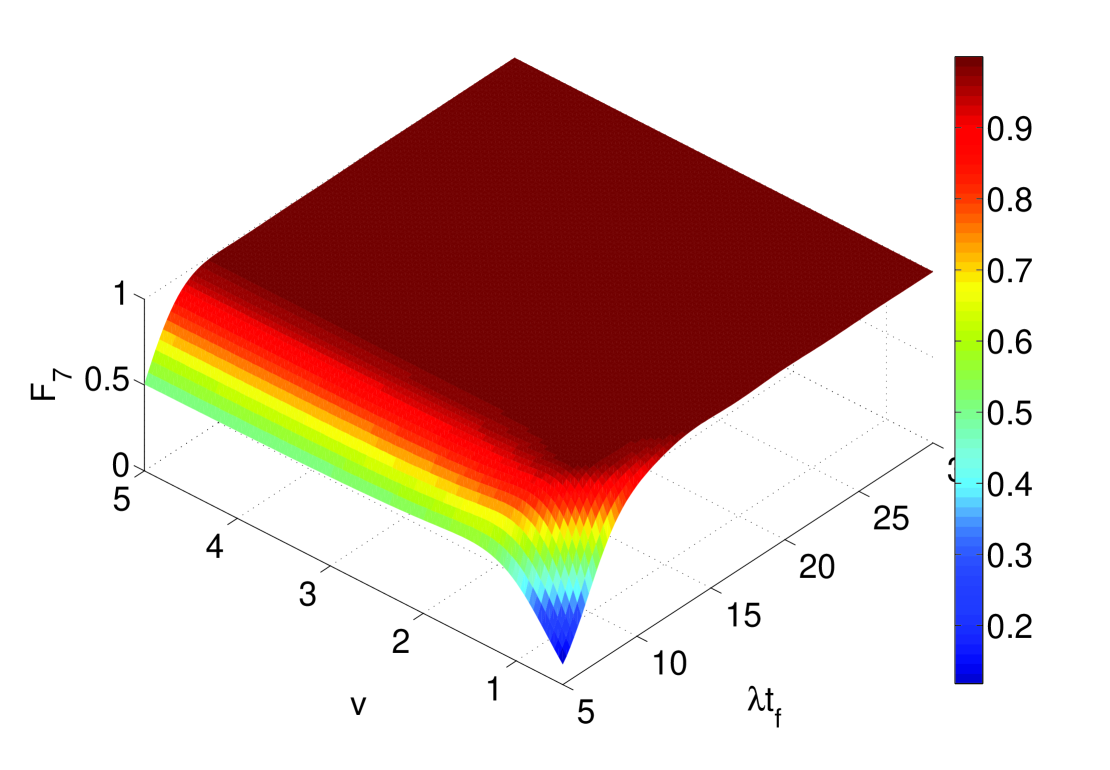
Figure 2: The fidelity of the target state $F_{7}$ versus parameters $v$ and $\lambda t_{f}$.

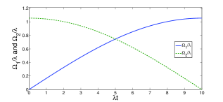
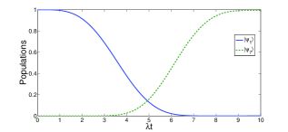
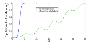
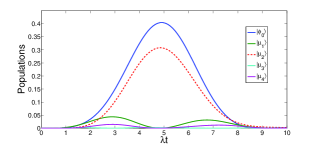
FIG. 3: (a) Dependence on $\lambda t$ of $\Omega_{1}(t)/\lambda$ and $\Omega_{2}(t)/\lambda$. (b) Dependence on $\lambda t$ of the populations for the initial state $|\psi_{1}\rangle$ and the target state $|\psi_{7}\rangle$. (c) The comparison of the operation times required for achieving the target state via adiabatic method with that via the present STAP method. (d) Dependence on $\lambda t$ of the populations for the intermediate states.

We will first analyze the relation between the cavity-fiber coupling $v$ and the interaction time $t_{f}$ as $v$ plays a great important role in the evolution. The fidelity $F_{7}$ of the target state $|\psi_{7}\rangle$ versus $v$ and $\lambda t_{f}$ is shown in Fig. 2 when $\epsilon=\arcsin{0.25}$, where the fidelity of a state is given through the relation $F=|\langle\psi|\rho(t_{f})|\psi\rangle|$. Figure 2 shows increasing the value of $v$ does not help to shorten the interaction time, which is different from what we mentioned above in Sec. III. The reason is that the relation between the coupling $v$ and the amplitude of the laser pulses $\Omega_{0}$ at that time was not taken into consideration. Known from Refs. XCILARDGJGMPrl10 ; AdCPra11 ; XCETJGMPra11 ; XCJGMPra12 ; MLYXLTSJSNBAPra14 ; YHCYXQQCJSPRA14 , shortening the time requires increasing the amplitude of the laser pulses. The amplitude of the laser pulses in Eq. (49) inverses proportion to the coupling $v$, and the smaller the amplitude is, the longer the interaction time is. Consequently it is wise to choose $v=g$ in our method. What is more, Fig. 2 shows that in the present case, the shortest interaction time required for an ideal population transfer from $|\psi_{1}\rangle$ to $|\psi_{7}\rangle$ is only about $8/\lambda$. The time dependences of $\Omega_{1}(t)/\lambda$ and $\Omega_{2}(t)/\lambda$ are shown in Fig. 3 (a) versus $\lambda t$ when $\epsilon=\arcsin{0.25}$, $t_{f}=10/\lambda$ and $v=\lambda$. The amplitude of the laser pulses $\Omega_{0}$ is $1.05\lambda$ which meets the conditions mentioned above. And such an intensity is safe to assume linear optic models. Similar laser amplitude has been used and discussed in Refs. YHCYXQQCJSPRA14 ; ADBABRMTENHJKPrl07 ; LBCMYYGWLQHDXMLPra07 ; JSYXXDSHSSPra12 ; JSXDSQXMLLZYXHSSPra13 . In Ref. JSYXXDSHSSPra12 proposed by Song et al., even high drive intensity $\Omega_{0}=\sqrt{5\sqrt{2}}\lambda\approx 2.6591\lambda$ was used. Fig. 3 (b) shows the time evolution of the populations in states $|\psi_{1}\rangle$ and $|\psi_{7}\rangle$. We contrast the interaction time required for achieving the target state via adiabatic process with the present STAP method in Fig. 3 (c). The result obviously shows that the present STAP method effectively shorten the interaction time than the adiabatic method even with the same laser intensity (we choose $\Omega_{1}=\lambda\sin{\beta}$ and $\Omega_{2}=\lambda\cos{\beta}$ in the adiabatic method). A similar process in an adiabatic scheme in Ref. LBCMYYGWLQHDXMLPra07 shows that the interaction time required to achieve the target state is almost $t_{f}=250/\lambda$ when all the populations of the excited states should be restrained to reduce the influence of dissipation. To demonstrate the conditions for the STAP process are fulfilled, especially, the condition that the state $|\mu_{1}\rangle$ is negligible during the evolution, we plot Fig. 3 (d) in case of {$\epsilon=\arcsin{0.25},t_{f}=10/\lambda$}. We find that the states $|\mu_{3}\rangle$ and $|\mu_{4}\rangle$ remain negligible all the time and the state $|\mu_{1}\rangle$ is very slightly populated but still considered as negligible since the maximum value of its population is only $4.36\%$. Besides, from Eq. (26), it is evident that the population of the state $|\mu_{2}\rangle$ has a spacial relationship with $\lambda t_{f}$:

$$P=|\frac{\sqrt{2}\Omega_{1}\Omega_{2}}{N_{D}\lambda}|^{2}=|\frac{2C^{2}}{(\lambda t_{f})^{2}+2C^{2}}|,$$ (155)

where $C=(\chi\pi\cot{\epsilon}\sin{\beta}\cos{\beta})/2v$. Though the STAP process is constructed based on nonadiabatic processes, the dark state $|D\rangle$ still can approximatively describe the evolution of the system because the adiabatic condition has not been absolutely destroyed. That is also why Eq. (155) is still useful to describe the population of the state $|\mu_{2}\rangle$. And the result of Eq. (155) shows that there is an inverse relationship between $P$ and $\lambda t_{f}$, that means, increasing the population of the state $|\mu_{2}\rangle$ is a simple and effective way to shorten the interaction time. Moreover, we have mentioned above that the state $|\mu_{2}\rangle$ can only be transformed from the state $|\mu_{1}\rangle$. Therefore, under the premise of the negligible state $|\mu_{1}\rangle$ during the evolution, properly increasing the population of the state $|\mu_{1}\rangle$ is of helpful to shorten the interaction time (this result also applies to most of the adiabatic schemes when the decoherence is not taken into consideration).

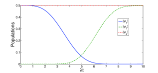
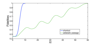
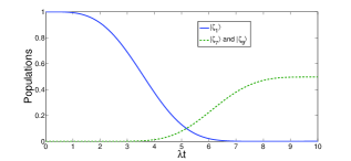
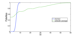
FIG. 4: (a) Time evolution of the populations for the states $|\phi_{1}\rangle$, $|\psi_{7}\rangle$, and $|\psi_{a}\rangle$ in the first scheme of Bell-state generation. (b) Time evolution of the fidelities of Bell stats via STAP and adiabatic methods. (c) Time evolution of the populations for the states $|\zeta_{1}\rangle$, $|\zeta_{7}\rangle$, and $|\zeta_{9}\rangle$ in the second scheme of Bell-state generation. (d) Time evolution of the fidelities of Bell stats via STAP and adiabatic methods.

In Fig. 4, we analyze the efficiency of the STAP for the generation of Bell entangled states. Figure. 4 (a) displays the time evolution of the populations in states $|\psi_{1}\rangle$, $|\psi_{7}\rangle$ and $|\psi_{a}\rangle$ in the first STAP for Bell-state generation, and we give a comparison between the performances of the fidelity of the two-atom Bell state based on the first STAP method for Bell-state generation and an adiabatic passage method governed by an Hamiltonian whose form is the same as that in Eq. (4) with parameters $\{\Omega_{1}=\lambda\sin{\beta},\Omega_{2}=\lambda\cos{\beta},t_{f}=60/\lambda\}$ satisfying the adiabatic condition. Figure. 4 (c) shows the populations in states $|\zeta_{1}\rangle$, $|\zeta_{7}\rangle$ and $|\zeta_{9}\rangle$ in the second STAP for Bell-state generation, and the second STAP method is contrasted with adiabatic passage method for the two-atom Bell state, demonstrating that the STAP method is much faster when one more atom is used. The green dashed curve in Fig. 4 (d) is plotted based on a model with two atoms trapped in a cavity whose interaction Hamiltonian is $H=\sum_{k=1,2}\Omega_{k}|e\rangle_{k}\langle f|+\lambda a|e\rangle_{k}\langle g|+H.c.$, and the parameters $\{\Omega_{1}=0.5\lambda(\sin{\beta})^{1.2},\Omega_{2}=\lambda(\cos{\beta})^{1.2},t_{f}=60/\lambda\}$ are set to satisfy the adiabatic condition. These models and parameters are chosen according to the principle of fair comparison. Both Figs. 4 (a) and (b), beyond doubt, give a result that the STAP methods can generate Bell-entangled states much faster than the adiabatic methods without requiring extra complex operations and harsh conditions.

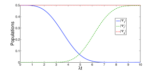
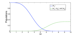
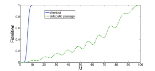
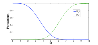
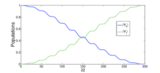
FIG. 5: Time-dependent populations in STAP schemes and the comparisons between STAP methods and adiabatic methods: (a) Time evolution of the populations for the states $|\Psi_{1}\rangle$, $|\Psi_{f}\rangle$ and $|\Psi_{a}\rangle$ of three-atom GHZ-state via STAP. (b) The comparison of total interaction times required between STAP method and adiabatic method for GHZ-state generation. (c) Time evolution of the populations for the states $|\Phi_{1}\rangle$, $|w_{1}\rangle$, $|w_{2}\rangle$ and $|w_{3}\rangle$ of three-atom $W$ via STAP. (d) The comparison of total interaction times required between STAP method and adiabatic method for $W$-state generation. (e) Time evolution of the entanglement transfer form the initial entangled state $|\Psi_{0}\rangle$ to target entangled state $|\Psi_{f}\rangle$ via STAP. (f) Time evolution of the entanglement transfer form the initial entangled state $|\Psi_{0}\rangle$ to target entangled state $|\Psi_{f}\rangle$ via adiabatic passage.

For simplicity, in the following when a comparison between the adiabatic method and the STAP method should be taken, the form of the Hamiltonian for an adiabatic method is chosen as the same as that for a STAP method. Figure. 5 (a) shows the time-dependent populations for states $|\Psi_{1}\rangle$, $|\Psi_{f}\rangle$ and $|\Psi_{a}\rangle$ in the scheme of fast GHZ state generation when $\{\epsilon=\arcsin{0.25},t_{f}=10/\lambda\}$, and Fig. 5 (b) gives the time comparison between the adiabatic method and the STAP method. The dashed curve in Fig. 5 (b) is plotted with parameters $\{\epsilon=\arcsin{0.02},t_{f}=60/\lambda\}$ satisfying the adiabatic condition via adiabatic passage. It is obvious that Figs. 5 (a) and (b) are almost as the same as Figs. 4 (a) and (b), respectively. Similar phenomenon is shown in the generation of $W$ state when we contrast Figs. 5 (c) and (d) with Figs. 4 (c) and (d). Here, Fig. 5 (c) displays the populations for states $|\Phi_{1}\rangle$, $|w_{1}\rangle$, $|w_{2}\rangle$, and $|w_{3}\rangle$ when $\{\epsilon=\arcsin{0.25},t_{f}=10/\lambda\}$, where $|w_{1}\rangle=|g\rangle_{p}|f,g,g\rangle_{1,2,3}|0,0,0\rangle_{c_{1},c_{2},f}$, $|w_{2}\rangle=|g\rangle_{p}|g,f,g\rangle_{1,2,3}|0,0,0\rangle_{c_{1},c_{2},f}$, and $|w_{3}\rangle=|g\rangle_{p}|g,g,f\rangle_{1,2,3}|0,0,0\rangle_{c_{1},c_{2},f}$, and Fig. 5 (d) gives the comparison between STAP method and adiabatic method for $W$ state generation. We choose parameters $\{\epsilon=\arcsin{0.02},t_{f}=100/\lambda\}$ to satisfy the adiabatic condition in the adiabatic method. As a matter of fact, the STAP methods for GHZ state and $W$ state generations are equivalent to the first and second STAP methods for Bell-state generations, respectively. When $M=2$, the STAP methods for $M$-particle-entangled-state generations are exactly the STAP methods for the Bell-state generations. From the result of analysis, a significant inference is obtained: the interaction time required for each of the generations of GHZ state and $W$ state is irrelevant to the number of qubits. Whereas, when there are too many atoms trapped in the cavity $c_{2}$, the system is possibly not safe to assume linear optic models since the couplings $\lambda_{s}$ is proportionally reduced while $\Omega_{s}(t)$ remains unchanged in Sec. IV C if we do not change the parameters. Therefore, in fact, the shortest interaction time required for $W$ state generation is limited by the number of qubits. But that only causes a small effect on the STAP method since even when $M=100$, we can still choose the interaction time as $t_{f}=50/\lambda$ which is still much shorter than that in an adiabatic method to make sure the system is safe to assume linear optic models (in this case, $\Omega_{0}\approx 2\lambda_{s}$). Figure 5 (e) shows the time evolution of the populations for the initial entangled state $|\Phi_{0}\rangle$ and target entangled state $|\Psi_{f}\rangle$ in the scheme of transition of two-atom entangled state when $\epsilon=\arcsin{0.25}$, $t_{f}=10/\lambda$ and $v=\lambda$. It is merited that Fig. 5 (e) is as the same as Fig. 3 (b), the reason for this phenomenon is also that the Hamiltonian in Eq. (143) is precisely the same to the Hamiltonian in Eq. (4). And Fig. 5 (f) is the two-atom entanglement transfer via adiabatic passage in case of $\{t_{f}=300/\lambda,\epsilon=\arcsin{0.02}\}$.

As is known to all, whether a scheme is applicable for quantum information processing and quantum computing depends on the robustness against possible mechanisms of decoherence. The dissipation has not been taken into account in the above discussion. And once the dissipation is considered, the evolution of the system can be modeled by a master equation in Lindblad form,

$$\dot{\rho}=i[\rho,H]+\sum_{k}[L_{k}\rho L_{k}^{{\dagger}}-\frac{1}{2}(L^{{\dagger}}_{k}L_{k}\rho+\rho L_{k}^{{\dagger}}L_{k})],$$ (156)

where the $L_{k}$’s are the so-called Lindblad operators. For the first scheme, there are seven Lindblad operators:

$$L_{1}^{\kappa_{c}} = \sqrt{\kappa_{1}}a_{1},L_{2}^{\kappa_{c}}=\sqrt{\kappa_{2}}a_{2},L_{3}^{\kappa_{f}}=\sqrt{\kappa_{f}}b,$$ (157)

$$L_{4}^{\Gamma} = \sqrt{\Gamma_{1}}|f\rangle_{1}\langle e|,L_{5}^{\Gamma}=\sqrt{\Gamma_{2}}|g\rangle_{1}\langle e|,L_{6}^{\Gamma}=\sqrt{\Gamma_{3}}|f\rangle_{2}\langle e|,L_{7}^{\Gamma}=\sqrt{\Gamma_{4}}|g\rangle_{2}\langle e|,$$ (158)

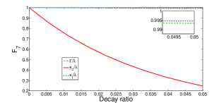
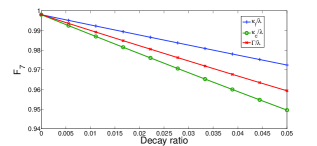
FIG. 6: (a) The influence of decays on the fidelity $F_{7}$ of the target state via adiabatic method: each of the three curves denotes $F_{7}$ versus each of the three noise resources when the other two are zero, for example the blue curve denotes the relationship between the fiber decay $\kappa_{f}/\lambda$ and the $F_{7}$ when $\kappa_{c}=\Gamma=0$. (b) The influence of decays on the fidelity $F_{7}$ of the target state via STAP method.

where $\kappa_{m}$ ($m=1,2$) are the decays of the cavities, $\kappa_{f}$ is the decay of the fiber, and $\Gamma_{n}$ ($n=1,2,3,4$) are the spontaneous emissions of atoms. We assume $\kappa_{m}=\kappa_{c}$ and $\Gamma_{n}=\Gamma/2$, in the interest of simplicity. Adiabatic passage technique has an advantage that the fidelity of the target state is independent of the fiber decay and atomic spontaneous emission because the intermediate states including the excited state of the fibers and atoms are always adiabatically eliminated, and the decoherence is usually caused by the cavity decay since the dark state always includes the terms including the cavity-excited states. We prove this by numerical simulation shown in Fig. 6 (a). Figure 6 (a) displays the fidelity $F_{7}$ versus each of the three noise resources when the other two are zero via adiabatic process (we choose parameters $\{\epsilon=0.02,t_{f}=100/\lambda\}$ to satisfy the adiabatic condition). Figure 6 (b) shows the relationship between $F_{7}$ and the three noise resources via STAP. Contrast these two figures; the benefits of the STAP method are shown obviously; though the STAP method is a little more sensitive to the fiber decay and atomic spontaneous emission, it is far more robust again the cavity decay than the adiabatic method. In a word, the STAP method is not only fast but also robust.

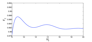
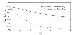
FIG. 7: (a) The relationship between the fidelity of the target state $|\psi_{7}\rangle$ and total interaction time $\lambda t_{f}$ in the presence of decoherence. (b) The maximum populations of states $|\phi_{0}\rangle$ and $|\mu_{2}\rangle$ versus the total interaction time $\lambda t_{f}$.

The decoherence, as a general rule, is dominated by the populations of the excited states and the total operation time. In the previous articles, the decoherence is always refrained by decreasing the populations of the excited sates. However, the excited states are required to speed up the transfer in the present STAP method. Therefore, we plot Fig. 7 (a) to demonstrate that in the present case, the decoherence is mainly dominated by the total operation time rather than the populations of the excited states. The result obviously shows that the fidelity is the highest when the operation time for achieving an ideal target state is the shortest i.e., $t_{f}=8.9/\lambda$. And the fidelity decreases gradually as $\lambda t_{f}$ increases while oscillating. When $t_{f}<8.9/\lambda$, as the conditions for constructing STAP are no longer faultlessly satisfied, the fidelity is lower than that when $t_{f}=8.9/\lambda$. The maximum populations of the intermediate states $|\phi_{0}\rangle$ and $|\mu_{2}\rangle$ which practically cause the decoherence versus $\lambda t_{f}$ are shown in Fig. 7 (b). The maximum populations clearly decrease with the increasing of $\lambda t_{f}$. Join up these two results, an inference is drawn, that is, at least when $9/\lambda\leq t_{f}\leq 20/\lambda$, the decoherence is mainly dominated by the total operation time since decreasing the populations of the excited sates does not obviously refrain the decoherence. Figure 7 (a) is plotted with parameters $\epsilon=\arcsin{0.25}$, $v=g$, and $\kappa_{c}=\kappa_{f}=\Gamma=0.05\lambda$, and Fig. 7 (b) is plotted with parameters $\epsilon=\arcsin{0.25}$, $v=g$, and $\kappa_{c}=\kappa_{f}=\Gamma=0$,

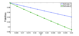
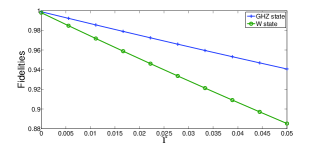
FIG. 8: (a) The fidelities of the Bell states versus the the ratios of decays by choosing $\Gamma/\lambda=\kappa_{f}/\lambda=\kappa_{c}/\lambda=\Upsilon$. (b) The fidelity of the three-atom GHZ state and the fidelity of the three-atom $W$ state versus the the ratios of decays by choosing $\Gamma/\lambda=\kappa_{f}/\lambda=\kappa_{c}/\lambda=\Upsilon$.

The robustness of the STAP for the Bell-state generations is shown in Fig. 8 (a) with $\Gamma/\lambda=\kappa_{f}/\lambda=\kappa_{c}/\lambda=\Upsilon$. And when we trap one more atom in the cavities, two more Lindblad operators $L_{n}^{\Gamma}=\sqrt{\Gamma_{n}}|S\rangle_{n}\langle e|$ ($S=f,g$) governing spontaneous emissions should be considered in the master equation. The result proves that the first STAP method for Bell-state generation is much more robust against decoherence than the second one. That is, because only the term $\frac{1}{\sqrt{2}}|\psi_{1}\rangle$ in Eq. (56) participates in the evolution. From such an initial state to the target state $\frac{1}{\sqrt{2}}|\psi_{7}\rangle$ along the STAP, the evolution is very closely analogous to the evolution of the FPT scheme in Sec. III except all of the coefficients of the states should be multiplied by $\frac{1}{\sqrt{2}}$. However, the second scheme of Bell-state generation is actually equivalent to the scheme for FPT. That means the population for each of the effective excited states in the second scheme is twice as large as that in the first scheme at any time during the evolution. Figure 8 (b) displays the fidelities of the three-atom GHZ and $W$ states versus the decays when $\Gamma/\lambda=\kappa_{f}/\lambda=\kappa_{c}/\lambda=\Upsilon$. Apparently Fig. 8 (b) is almost identical with Fig. 8 (a). Further research shows that, when it comes to the generations of more qubits GHZ and $W$ states, the robustness of the schemes against decoherence still remains the same as that of three atoms. It is implied that not only the interaction time required for the generation of entangled states but also the robustness of the scheme against decoherence is irrelevant to the number of qubits. The reason for this phenomenon is not hard to understand: however much atoms are trapped in the cavities, the photon emitted from the atom $1$ in the cavity $c_{1}$ can only excite one of atoms in cavity $c_{2}$. In other words, the holistic spontaneous emissions of $M$ atoms is equivalent to that of one atom in the cavity $c_{2}$. The result applies to the scheme of the transition of entangled states as well.

Finally, we present a brief discussion about the basic elements in the real experiment. The cesium atoms can be used to implement the schemes, the state $|g\rangle$ corresponds to $F=3$, $m=2$ hyperfine state of $6^{2}S_{1/2}$ electronic ground state, $|a\rangle$ corresponds to $F=3$, $m=4$ hyperfine state of $6^{2}S_{1/2}$ electronic ground state, $|f\rangle$ corresponds to $F=4$, $m=3$ hyperfine state of $6^{2}S_{1/2}$ electronic ground state, and $|e\rangle$ corresponds to $F=4$, $m=3$ hyperfine state of $6^{2}P_{1/2}$ electronic state. An almost perfect fiber-cavity coupling with an efficiency larger than $99.9\%$ can be realized using fiber-taper coupling to high-Q silica microspheres SMSTJKOJPKJVPrl03 . The fiber loss at $852$-nm wavelength is only about $2.2$ dB/Km KJGVFPDTGSBIeee04 , in this case, the fiber decay rate is only $0.152$ MHz. While in recent experimental conditions JRBHJKPra03 ; SMSTJKKJVKWGEWHJKPra05 , it is predicted to achieve a strong atom-cavity coupling $\lambda=2\pi\times 750$ MHz. That means the fiber decay can actually be neglected in a real experiment with these parameters. And by choosing another set of parameters $(\lambda,\Gamma,\kappa_{c})=(2500,10,10)$ MHz in the microsphere cavity QED experiment reported in SMSTJKKJVKWGEWHJKPra05 ; MJHFGSLBMBPNat06 , the fidelities of all of the STAP schemes in this paper are higher than $99\%$.

Till now, all the above description and discussion are based on atoms are trapped in two distant cavities which are connected by a fiber, in fact, the present STAP can also be generalized to the system with $N$ ($N\geq 2$) atoms respective trapped in $N$ cavities which are connected by $N-1$ fibers SYHYXJSNBAJosab13 . In such a system, there exist only one eigenvector whose eigenvalue is zero for the intermediate Hamiltonian and one dark state. Similar to Eqs. (18 - 30) in Sec. III, in light of quantum Zeno subspace division, we can rewrite the interaction Hamiltonian with some special vectors and partition the intermediate states into parts which are independent of each other. After discarding most of the parts except $S_{0}$ and $S_{1}$ whose eigenvalues are Zero and closest to zero, respectively, the effective Hamiltonian which has the same form as that in Eq. (30) is easily obtained, and then the STAP can also be constructed to realize the fast and noise-resistant population transfer, quantum entangled states preparation, and quantum entangled states transition in multi-cavity-fiber-atom combined system.

VII Conclusion

“Shortcuts to adiabatic process” provides alternative fast and robust processes which reproduce the same final populations, or even the same final state, as the adiabatic process in a finite, shorter time. In general, the operation time for a method is the shorter the better, otherwise, the method may be useless. Many experiments of quantum information science also desire fast and robust theoretical methods since high repetition rates contribute to the achievement of better signal-to-noise ratios and better accuracy. Therefore, in this paper, through dividing the whole system into parts, we construct shortcuts in different parts in the same time, and implement the fast quantum information processing via the STAP. Different schemes are proposed to perform fast population transfer, entanglement states generations, and entangled states transition. Through using the STAP, the problem of proposing effective schemes which are not only fast, but also robust to perform population transfer, prepare entanglements and implement entangled states transition in multi-cavity-fiber-atom combined system have been successfully overcome. Numerical simulation demonstrates the all of schemes are fast and robust versus variations in the experimental parameters and decoherence. Moreover, similar operations can also be applied to other cavities QED systems, for example, multi-cavity-cavity coupled system, to realize fast and noise-resistant quantum information processing. We believe that the present work is promising and will make great contributions to the experimental research in quantum information science. ($\sim 93\%$)

VIII ACKNOWLEDGEMENT

This work was supported by the National Natural Science Foundation of China under Grants No. 11105030 and No. 11374054, the Major State Basic Research Development Program of China under Grant No. 2012CB921601, and the Foundation of Ministry of Education of China under Grant No. 212085.

Figure 1: (a) The set-up diagram. (b) The atomic level configuration for the $\Lambda$-type atom. (c) The atomic level configuration for the atoms with the auxiliary ground state $|a\rangle$ in the schemes of Bell-state and GHZ-state generations.

References

- (1) J. S. Bell, Physics (Long Island City, NY) 1, 195 (1964).
- (2) D. M. Greenberger, M. A. Horne, A. Shimony, and A. Zeilinger, Am. J. Phys. 58, 1131 (1990).
- (3) E. Collin, G. Ithier, A. Aassime, P. Joyez, D. Vion, and D. Esteve, Phys. Rev. Lett. 93, 157005 (2004).
- (4) B. T. Torosov, D. Guérin, and N. V. Vitanov, Phys. Rev. Lett. 106, 233001 (2011).
- (5) L. Allen and J. H. Eberly, Optical Resonance and Two-Level Atoms (New York: Dover) pp 102-3 (1987).
- (6) K. Bergmann, H. Theuer, and B. W. Shore, Rev. Mod. Phys. 70, 1003 (1998).
- (7) N. V. Vitanov, T. Halfmann, B. W. Shore, and K. Bergmann, Annu. Rev. Phys. Chem. 52, 763 (2001).
- (8) P. Král, I. Thanopulos, and M. Shapiro, Rev. Mod. Phys. 79, 53 (2007).
- (9) X. Chen, I. Lizuain, A. Ruschhaupt, D. Guéry-Odelin, and J. G. Muga, Phys. Rev. Lett. 105, 123003 (2010).
- (10) E. Torrontegui, S. Ibáñez, S. Martínez-Garaot, M. Modugno, A. del Campo, D. Gué-Odelin, A. Ruschhaupt, X. Chen, and J. G. Muga, Adv. Atom. Mol. Opt. Phys. 62, 117 (2013).
- (11) A. Ruschhaupt, X. Chen, D. Alonso, and J. G. Muga, New J. Phys. 14, 093040 (2012).
- (12) A. del Campo, Phys. Rev. A 84, 031606(R) (2011).
- (13) X. Chen, E. Torrontegui, and J. G. Muga, Phys. Rev. A 83, 062116 (2011).
- (14) X. Chen and J. G. Muga, Phys. Rev. A 86, 033405 (2012).
- (15) M. Demirplak and S. A. Rice, J. Phys. Chem. A 107, 9937 (2003); J. Phys. Chem. B 109, 6838 (2005); J. Chem. Phys. 129, 15411 (2008).
- (16) M. B. Berry, J. Phys. A: Math. Theor. 42, 365303 (2009).
- (17) J. F. Schaff, X. L. Song, P. Vignolo, G. Labeyrie, Phys. Rev. A 82, 033430 (2010).
- (18) J. F. Schaff, X. L. Song, P. Capuzzi, P. Vignolo, G. Labeyrie, Euro. Phys. Lett. 93, 23001 (2011).
- (19) A. Walther, F. Ziesel, T. Ruster, S. T. Dawkins, K. Ott, M. Hettrich, K. Singer, F. Schmidt-Kaler, and U. Poschinger, Phys. Rev. Lett. 109, 080501 (2012).
- (20) R. Bowler, J. Gaebler, Y. Lin, T. R. Tan, D. Hanneke, J. D. Jost, J. P. Home, D. Leibfried, D. J. Wineland, Phys. Rev. Lett. 109, 080502 (2012).
- (21) S. Y. Tseng, X. Chen, Optic. Lett. 37, 5118 (2012).
- (22) M. G. Bason, M. Viteau, N. Malossi, P. Huillery, E. Arimondo, D. Ciampini, R. Fazio, V. Giovannetti, R. Mannella, O. Morsch, Nature Physics 8, 147 (2012).
- (23) M. Lu, Y. Xia, L. T. Shen, J. Song, and N. B. An, Phys. Rev. A 89, 012325 (2014).
- (24) M. Lu, L. T. Shen, Y. Xia, and J. Song, Laser Phys. (Accepted) (2014).
- (25) Y. H. Chen, Y. Xia, Q. Q. Chen, and J. Song, Phys. Rev. A 89, 033856 (2014).
- (26) X. Shi and L. F. Wei, arXiv:1309.3020v1 (2013).
- (27) J. M. Raimond, M. Brune, and S. Haroche, Rev. Mod. Phys. 73, 565 (2001).
- (28) M. A. Sillanp et al., Nature 449, 438 (2007).
- (29) J. Majer et al., Nature 449, 443 (2007).
- (30) H. J. Kimble, Nature 453, 1023 (2008).
- (31) J. S. Bell, Physics 1, 195 (1964).
- (32) D. M. Greenberger, M. Horne, A. Shimony, and A. Zeilinger, Am. J. Phys. 58, 1131 (1990).
- (33) W. Dür, G. Vidal, and J. I. Cirac, Phys. Rev. A 62, 062314 (2000).
- (34) C. H. Bennett, G. Brassard, and C. Crépeau, Phys. Rev. Lett. 70, 13 (1993).
- (35) B. S. Shi, Y. K. Jiang, and G. C. Guo, Phys. Lett. A 268, 161 (2000).
- (36) J. I. Cirac, P. Zoller, H. J. Kimble, and H. Mabuchi, Phys. Rev. Lett. 78, 16 (1997).
- (37) Z. Q. Yin and F. L. Li, Phys. Rev. A 75, 012324 (2007).
- (38) S. B. Zheng and G. C. Guo, Phys. Rev. Lett. 85, 2392 (2000).
- (39) H. R. Lewis and W. B. Riesenfeld, J. Math. Phys. 10, 1458 (1969).
- (40) M. A. Lohe, J. Phys. A: Math. and Theor. 42, 035307 (2009).
- (41) T. Pellizzari, Phys. Rev. Lett. 79, 5242 (1997).
- (42) A. Serafini, S. Mancini, and S. Bose, Phys. Rev. Lett. 96, 010503 (2006).
- (43) P. Facchi and S. Pascazio, Phys. Rev. Lett. 89, 080401 (2002).
- (44) Y. Z. Lai, J. Q. Liang, H. J. W. Müller-Kirsten, and J. G. Zhou, Phys. Rev. A 53, 3691 (1996); J. Phys. A 29, 1773 (1996).
- (45) A. D. Boozer, A. Boca, R. Miller, T. E. Northup, and H. J. Kimble, Phys. Rev. Lett. 98, 193601 (2007).
- (46) L. B. Chen, M. Y. Ye, G. W. Lin, Q. H. Du, and X. M. Lin, Phys. Rev. A 76, 062304 (2007).
- (47) J. Song, Y. Xia, X. D. Sun, and H. S. Song, Phys. Rev. A 86, 034303 (2012).
- (48) J. Song, X. D. Sun, Q. X. Mu, L. L. Zhang, Y. Xia, and H. S. Song, Phys. Rev. A 88, 024305 (2013).
- (49) S. .M. Spillane, T. J. Kippenberg, O. J. Painter, and K. J. Vahala, Phys. Rev. Lett. 91, 043902 (2003).
- (50) K. J. Gordon, V. Fernandez, P. D. Townsend, and G. S. Buller, IEEE J. Quantum Electron. 40, 900 (2004).
- (51) J. R. Buck and H. J. Kimble, Phys. Rev. A 67, 033806 (2003).
- (52) S. M. Spillane, T. J. Kippenberg, K. J. Vahala, K. W. Goh, E. Wilcut, and H. J. Kimble, Phys. Rev. A 71, 013817 (2005).
- (53) M. J. Hartmann, F. G. S. L. Brandão, and M. B. Plenio, Nat. Phys. 2, 849 (2006).
- (54) S. Y. Hao, Y. Xia, J. Song, and N. B. An, J. Opt. Soc. Am. B 30, 2 (2013).